Article

A New Visual Inertial Simultaneous Localization and Mapping (SLAM) Algorithm Based on Point and Line Features

1
Unmanned System Research Institute, Northwestern Polytechnical University, Xi’an 710072, China
2
System Engineering Institute of Sichuan Aerospace, Chengdu 610100, China
3
School of Astronautics, Northwestern Polytechnical University, Xi’an 710072, China
*
Author to whom correspondence should be addressed.
Drones 2022, 6(1), 23; https://doi.org/10.3390/drones6010023
Submission received: 12 November 2021 / Revised: 9 January 2022 / Accepted: 10 January 2022 / Published: 13 January 2022
(This article belongs to the Special Issue Advances in SLAM and Data Fusion for UAVs/Drones)

Abstract

:
In view of traditional point-line feature visual inertial simultaneous localization and mapping (SLAM) system, which has weak performance in accuracy so that it cannot be processed in real time under the condition of weak indoor texture and light and shade change, this paper proposes an inertial SLAM method based on point-line vision for indoor weak texture and illumination. Firstly, based on Bilateral Filtering, we apply the Speeded Up Robust Features (SURF) point feature extraction and Fast Nearest neighbor (FLANN) algorithms to improve the robustness of point feature extraction result. Secondly, we establish a minimum density threshold and length suppression parameter selection strategy of line feature, and take the geometric constraint line feature matching into consideration to improve the efficiency of processing line feature. And the parameters and biases of visual inertia are initialized based on maximum posterior estimation method. Finally, the simulation experiments are compared with the traditional tightly-coupled monocular visual–inertial odometry using point and line features (PL-VIO) algorithm. The simulation results demonstrate that the proposed an inertial SLAM method based on point-line vision for indoor weak texture and illumination can be effectively operated in real time, and its positioning accuracy is 22% higher on average and 40% higher in the scenario that illumination changes and blurred image.

1. Introduction

In recent decades, visual simultaneous localization and mapping (SLAM) [1] algorithm is regarded as the core technique to achieve a mobile robot’s autonomous operation. Its appearance enables mobile robots to obtain their own state and surrounding environmental information through corresponding sensors in indoor environments with weak GPS signals, so as to realize map construction and environmental cognition and complete specific tasks autonomously.
According to the coupling mode of vision and IMU, visual inertial SLAM system can be divided into two types: loosely coupled and tightly coupled. The loosely coupled method is the result of motion estimation independently by integrating the two modules of vision and IMU, such as [2,3], while the tightly coupled method uses the original data of camera and IMU to combine for optimization, which makes it easier to obtain globally consistent estimation results.
Classical tightly coupled SLAM frameworks include VINS-Mono [4] and ORB-Slam2 [5]. Based on these two frameworks, researchers have proposed many improved versions [6,7]. Point feature is the most commonly used feature type of the above algorithms, but point feature algorithms such as the Scale Invariant Feature Transform (SIFT) [8], Features from Accelerated Segment Test (FAST) [9] and the Ori-ented FAST and Rotated BRIEF (ORB) [10] have difficulty in detecting sufficient numbers of point features on the scenes of poor texture such as corridor, window or white wall. In addition, owing to the quick movement of a camera, poor texture, illumination change and so on, point feature matching’s quality and quantity may decrease greatly.
One of the effective solutions to solve the above problems is to add line features. Compared with point features, the indoor artificial scenes have plentiful edges, linear structures and obvious line features. The line features have better illumination invariance and rotation constancy, so they may provide more geometric structural information and enhance the robustness and accuracy of the SLAM algorithm based on a single point feature.
Vakhitov et al. [11] proposed the EPn-PL and OPnPL algorithm that combines point and line features. Zuo et al. [12] attempted to use the Pruck coordinates to show the line features in the front-end SLAM algorithm, which combines point and line features, but they used the smallest orthogonality to show the parameterized line features in the back-end optimization algorithm. Pumarola et al. [13] added line features to the basis of the ORB-SLAM algorithm and proposed using line features to initialize the algorithm. For the first time, Gomez-Ojeda et al. [14] developed the open-source SLAM algorithm based on double-purpose point and line features, which weigh and fully consider point and line features in the loop detection module. At present, studies based on the combination of point-line features are mainly represented by PL-VIO [15], PLS-VIO [16], PL-VINS [17], etc. However, the running efficiency of SLAM system based on point and line features is easily affected by the front-end algorithm because features of every frame of image need to be extracted and matched. The introduction of line feature increases the time consumption of feature extraction and matching, which reduces the operating efficiency and stability of SLAM system.
Aiming at the above problems, an indoor visual inertial SLAM algorithm based on point-line feature is proposed. By adopting bilateral filtering algorithm and SURF [18] feature extraction algorithm, the system has a stronger ability to resist light changes. The fast nearest neighbor algorithm is used for feature matching, and the matching accuracy is higher than the original SLAM system. Compared with the original SLAM system based on point-line feature, our method has higher accuracy. Line Segment Detector (LSD) [19] algorithm was adjusted to solve the problem of large computation and inefficiency. At the same time, we change the original complex matching process. Geometric constraints and random sampling consistency algorithm are used to reduce the computation of feature matching process to improve the real-time performance of the system. And step joint initialization is used to improve the stability of the algorithm. The purpose of this study is to improve the real-time performance, stability and accuracy of SLAM systems in complex environments.
The rest of the paper is organized as follows. The algorithm framework is proposed in Section 2. Section 3 proposes the image processing method in detail and describes the initialization work. Lastly, the experimental result is presented in Section 4 to verify the advantage in Section 3.

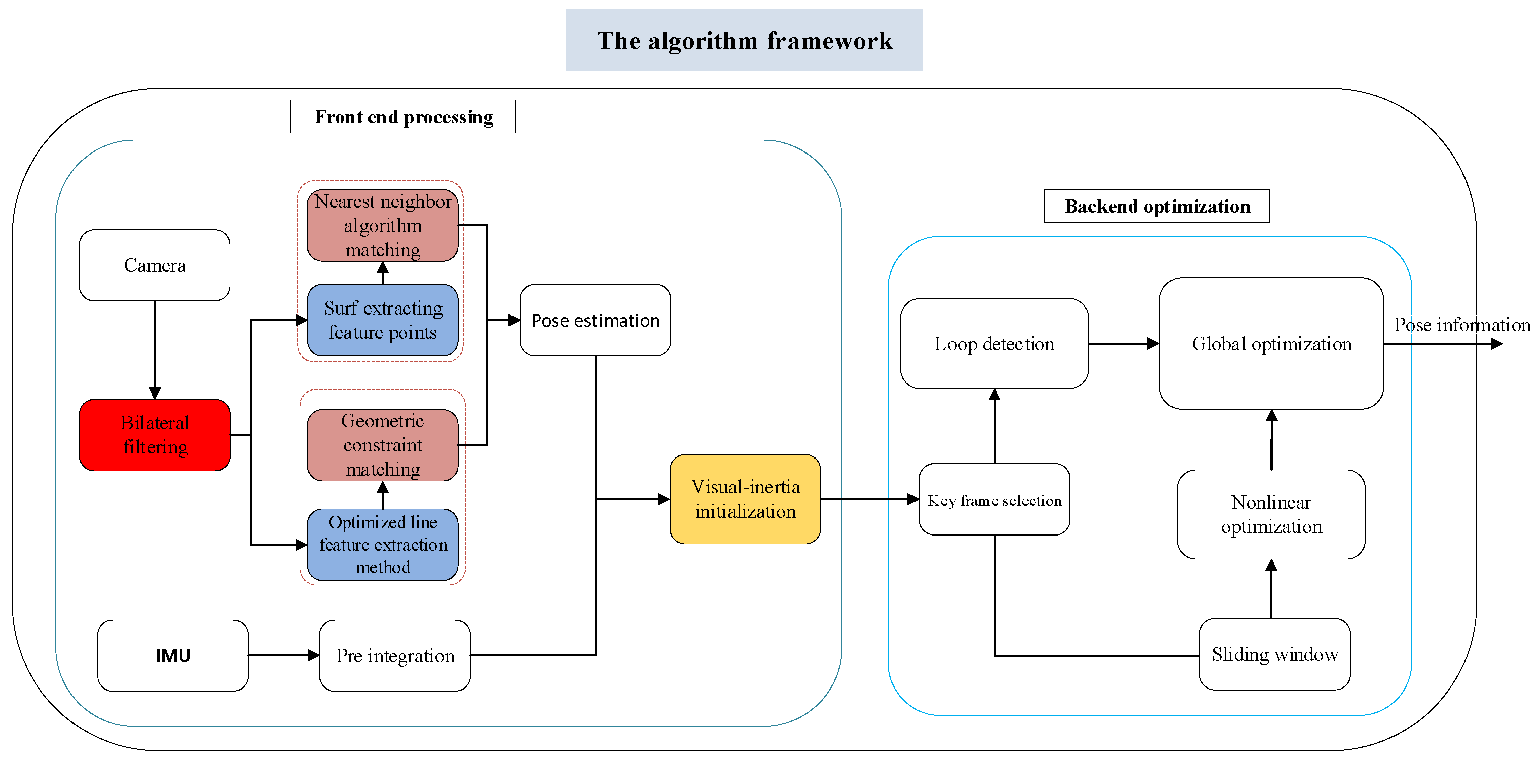
2. The Algorithm Framework

This paper mainly studies image processing algorithm and visual inertial initialization algorithm at front-end, and the traditional nonlinear optimization framework at back-end. The main contribution is the colored part in Figure 1. As shown in Figure 1, the algorithm is established based on the PL-VIO algorithm. This study focuses on the point and line feature extraction and matching algorithms of data preprocessing module:
(1)
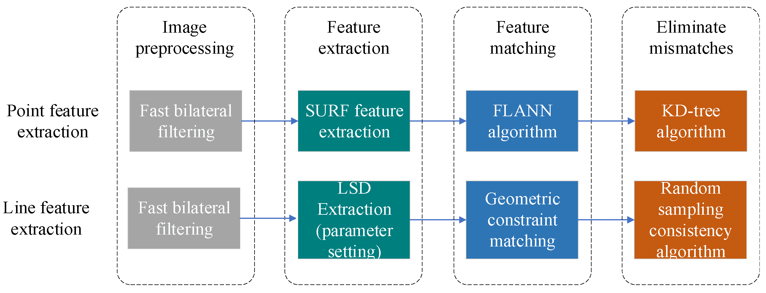
The SURF algorithm can extract stable features even at the circumstances of translation, rotation and perspective change, so this paper uses the SURF algorithm to extract point features. The traditional optical flow tracking method is not suitable for the environment with drastic light changes. The matching algorithm used in this paper is the fast nearest-neighbor algorithm (FLNN) [20], which can link to the SURF parameters.
(2)
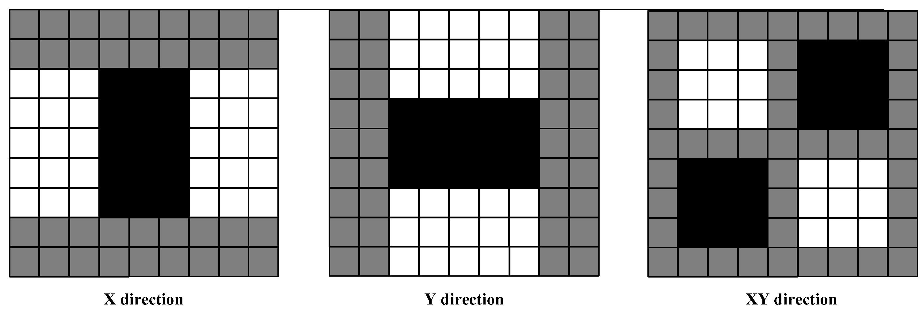
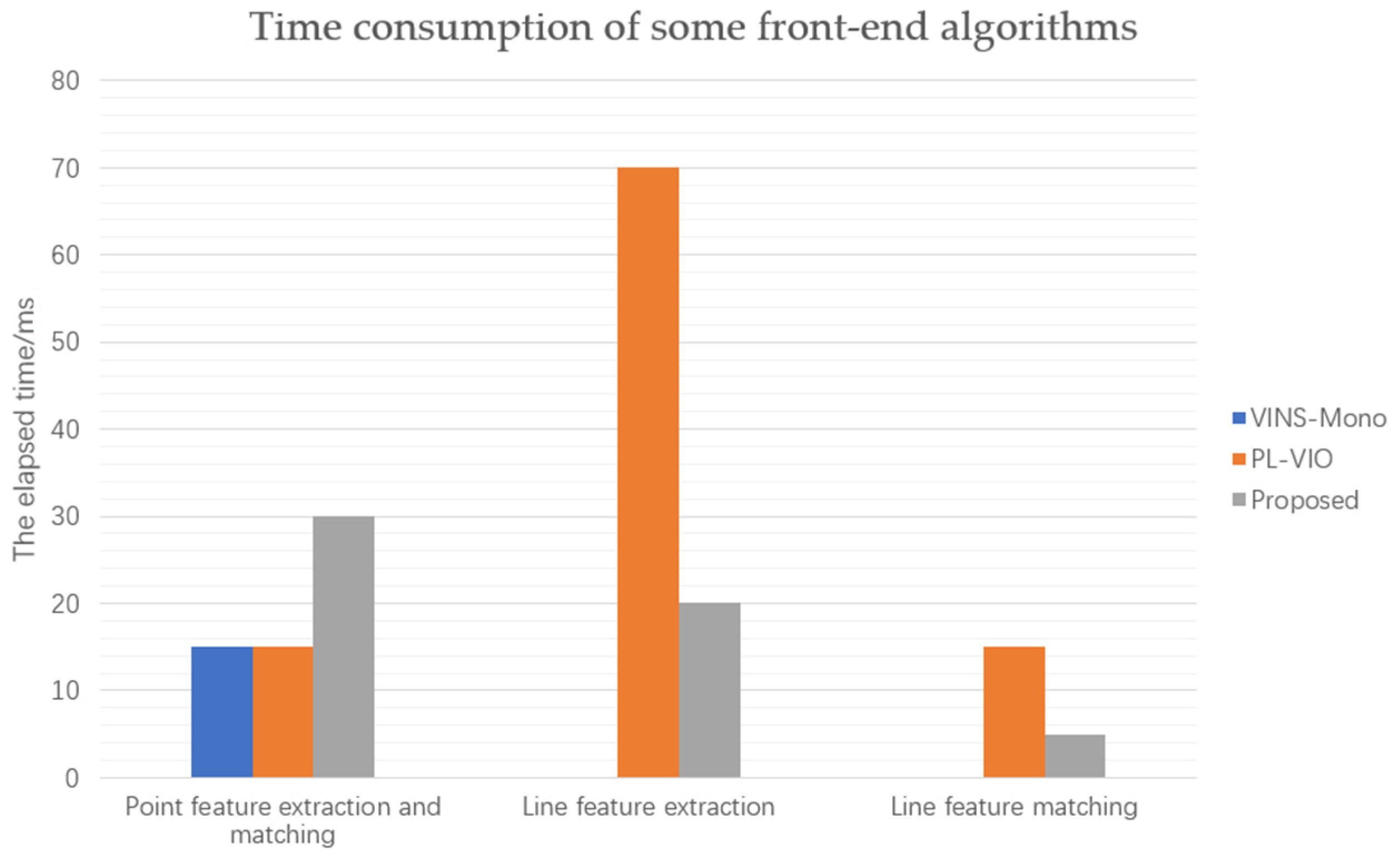
In terms of online feature extraction and matching, LSD algorithm was initially proposed to describe the contour of the object, which is not suitable for line segment positioning in space. Therefore, the parameters of LSD algorithm need to be adjusted, and an adaptive line segment constraint method is proposed to greatly reduce the time required for line feature matching. Based on the work of Gomez-Ojed [21], a constraint method of pole-geometry and point-line affine invariants is proposed to improve the speed of line feature processing.
(3)
Point-line feature SLAM based on nonlinear optimization has the defects of long inertial initialization time and poor stability. In this paper, a step-by-step joint initialization [21] method is used to improve stability and reduce initialization time.

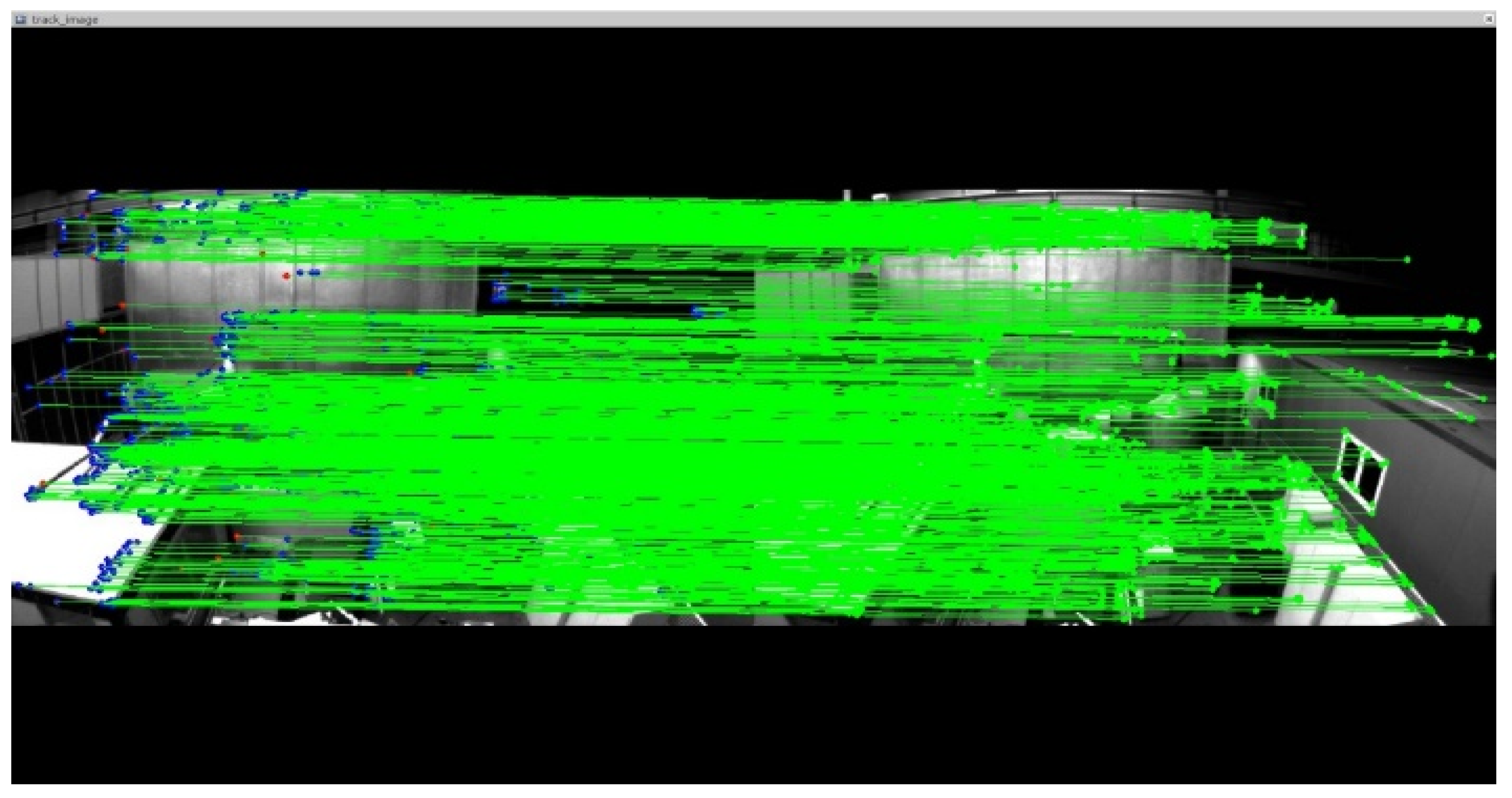
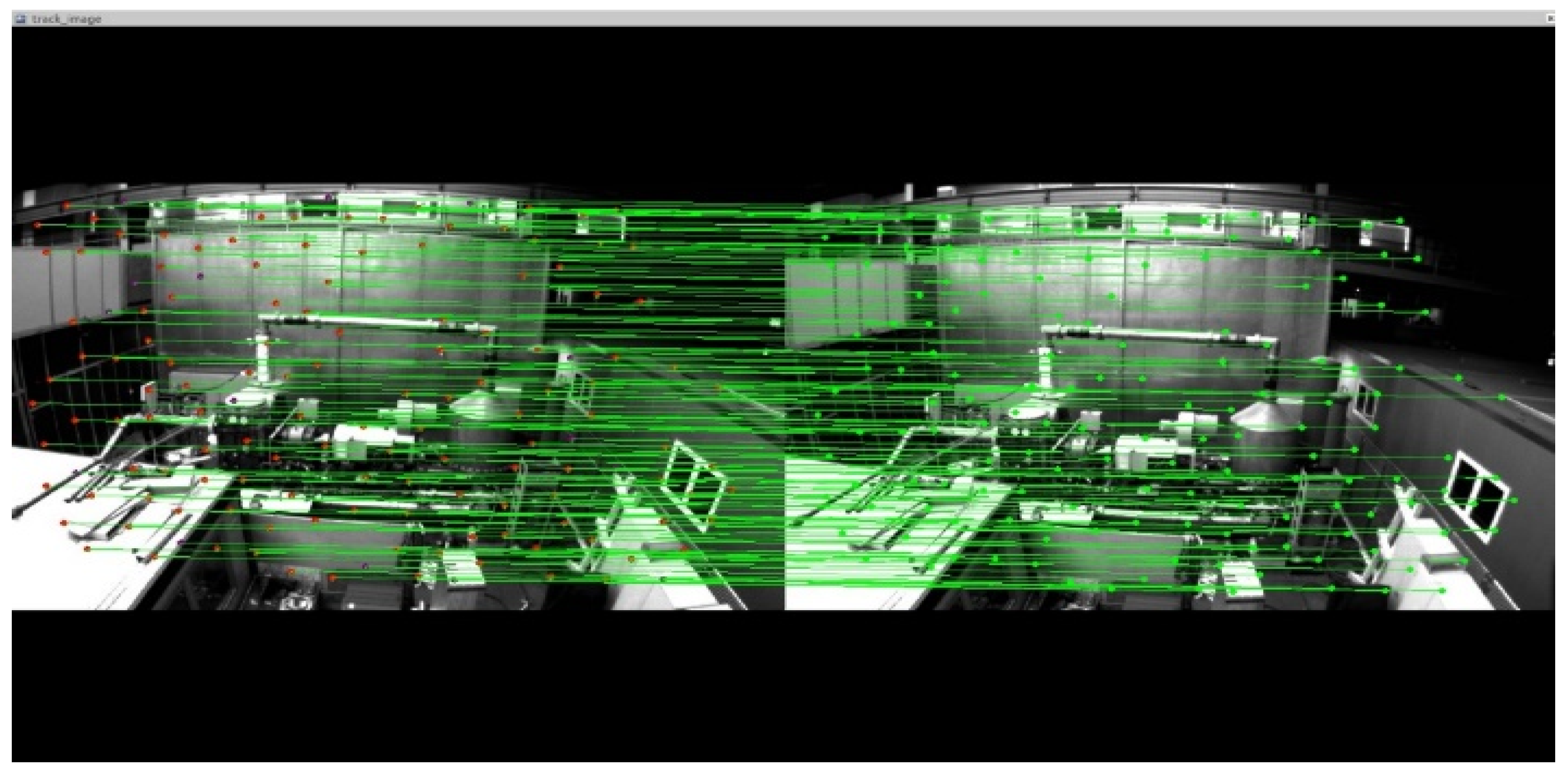
3. Front End Processing

The processing flow chart of point and line features is shown in Figure 2.

3.1. The Image Processing

Noise and some other pseudo-point features and lines need to be eliminated before the extraction of point and line features. Considering the spatial proximity and gray-scale similarity between pixel points and the surrounding pixel strips, we use bilateral filtering to process [21]. Edge preservation of bilateral filtering is achieved by combining spatial and range kernel functions during convolution, as shown below:
H I = 1 W x N G σ d ( x y ) G σ r ( I x I y ) I y
where
W = x N G σ d ( x y ) G σ r ( I x I y ) G σ d = e 1 2 ( d ( x , y ) σ d ) 2 G σ r = e 1 2 ( δ ( I x , I y ) σ r ) 2
y is the pixel to be obtained, N is the square neighborhood centered on pixel y in image I , and x is any other pixel in the neighborhood, I x , I y is the number of pixels, G σ d is the spatial neighbor-domain relational function, x y is the spatial distance, G σ r is the grey-scale value resemblance function, σ d is the standard deviation of spatial Gaussian function and σ r is the standard deviation of the range Gaussian function, d   ( x ,   y ) and   δ   ( I x ,   I y ) represent the Euclidean distance of pixel points x and y , respectively and the gray difference of pixel values I x and I y .
Thus, in the flat area of the image, the value of I x I y changes very little, and the corresponding range weight is close to 1. At this time, the spatial domain weight plays a major role, which is equivalent to directly Gaussian blurring of this area. In the edge area, I x I y will have a large difference, and then the domain coefficient will decrease, resulting in a decrease in the distribution of the entire kernel function here, while maintaining the details of the edge.
The SURF operator is based on scale space detection and uses a Gaussian filtered Hessian matrix to extract point features. The Hessian matrix of image point   I ( x , y ) with scale σ is defined as:
H ( I , σ ) = [ L x x ( I , σ ) L x y ( I , σ ) L x y ( I , σ ) L y y ( I , σ ) ]
where L x x ( I , σ ) , L x y ( I , σ ) and L y y ( I , σ ) are the two-dimensional convolution of the image by the Gaussian second-order differential at point I .
Surf uses Box filter to approximately replace Gaussian filter. The image filtering problem of Box filter is transformed into the calculation of the addition and subtraction of pixel sum between different regions of the image, which can be completed by simply searching the integral graph for several times. An approximation of the determinant of the Hessian matrix [18] for each pixel:
det ( H ) = D x x ( x ) D y y ( x ) ( 0 . 9 D x y ( x ) ) 2
The algorithm uses a Box filter to approximately replace the Gaussian filter. Therefore, it multiplies D x y with the weight coefficient 0.9 so as to even out the errors caused by the Box filter. In discrete image pixels, an image processing template can be used instead. For example, the templates in X direction, Y direction and XY direction are shown in Figure 3. We calculate D x x through the template in X direction, D y y through the template in Y direction and D x y through the template in X Y direction. Finally, the value of the determinant of the Hessian matrix for each pixel can be obtained by taking it into Formula (4).
Box filter image processing template [18] is as below.
The raw image is used to create its pyramids of various scales through enlarging the size of a square frame filter; then an integral image is used to accelerate its convolution, the further solution of which produces the determinants of the fast Hessian matrix. Experiments show that when the size of the box filter is enlarged twice, that is, when the pyramid model is set to 2, the operation time and effect of feature extraction are optimal.
In the point feature extraction algorithm, the Hessian value of the SURF is set to 800, and the results of the original extraction algorithm are shown in Figure 4. After the bilateral filtering of the SURF algorithm is shown in Figure 5, the reduction of invalid point features on the white wall and ground can be seen.
In this paper, the FLANN algorithm is used to match features, and the implementation steps of FLANN algorithm are as follows:
(1)
Using the point features of the first image as the training set and the point features of the second image as the query set, the Euclidean distances between all the point features in the training set and the point features in the query set are obtained.
(2)
By comparing Euclidean distances, the closest and second closest points of Euclidean distance between each point feature of training set and point feature of query set are preserved, and the remaining matches are discarded. Euclidean distance is:
D ( x , y ) = x , y = i = 1 d ( X i Y i ) 2
(3)
If the nearest Euclidean distance and the sub-nearest Euclidean distance satisfy Formula (6) keep the matching pair, otherwise delete the matching pair. Wherein, ratio is the threshold for judging the difference between the matching pair of the nearest Euclidean distance and the matching pair of the sub-nearest Euclidean distance (0 < ratio < 1). The larger the ratio, the more matching pairs, and the lower the matching accuracy. The smaller the ratio value, the fewer matching pairs, and the higher matching accuracy. Through experiments, it is found that when the ratio is 0.6, the number of point feature matching can reach 150, and the error of matching is small.
Nearest   Euclidean   Distance Sub - near   Euclidean   distance < r a t i o
As shown in Figure 6, SURF-based feature matching has a large number, but mismatching still exists. The matching results based on the algorithm in this paper are shown in Figure 7. Obviously, after the addition of FLANN algorithm, partial mismatching and redundant point features are eliminated, and the point feature matching effect is better.
Setting appropriate internal parameters of LSD such as pyramid number, scale factor and minimum density threshold can significantly improve the extraction speed. Through verification, the extraction process can be accelerated when the number of pyramid layers N is 3, the scale factor is 0.5 and the minimum density threshold is 0.5.
In order to improve the quality of line feature extraction, the length threshold was set to screen out the long line segments that were conducive to pose estimation, and the unstable short line segments that contributed little to pose estimation were eliminated. The length of a line segment must meet the following conditions:
{ l e n l i { l e n min = β [ max ( W I , H I ) ] } , i { 1 , 2 , , k } β = 1 e 0.001 k
where l e n l i is the length of the line segment i , l e n min is the shortest segment length, W I is the input image frame width, H I is the height of the input image frame, the symbol represents an upward rounding, β represents a length factor, k represents the number of line features extracted by the current frame.
Pl-VINS [17] uses a similar strategy to improve the quality of line segments, but it only selects length factors empirically, which is not applicable to the situation where the number of line segments varies greatly. If the selected value of length factor is large, the number of effective tracking line segments is insufficient when the number of line segments is small. If the selected value is small, redundant short line segments cannot be effectively eliminated when there are many line segments. In this paper, the number of line segments is mapped to the length factor by formula β = 1 e 0.001 k . When the number of line segments is small, the length threshold is increased to obtain more line segments for inter-frame tracking. When the number of line segments is large, reducing the length threshold reduces the influence of short line segments on the stability of pose estimation, which improves the adaptability of the length threshold screening strategy under different number of line segments. Finally, the speed of line feature extraction is three times of the original LSD algorithm before adjustment.
This paper presents a line feature matching method based on geometric constraints. Define segments l k = { s k , e k } , s k and e k as the start and end of the segment respectively. Let the reference line segment be l i , the query line segment be l j , and the line segment pair to be matched is ( l i , l j ) . The parallel relationship between the line segment pairs is represented by the included angle θ i j of the line segment pair:
θ i j = a r c tan ( I i × I j / I i I j )   ,   I k = s k e k s k e k 2
The constraints on polar geometry are expressed by the angle between the midpoint flow x i j = m i   m j , m k = (   s k + e k ) / 2 of a line segment and the coordinate axis in a two-dimensional coordinate system. In inter-frame matching, the corresponding pole-to-pole geometry constraint is:
θ i j f = arcsin ( x i j × η y / x i j )
θ i j s and θ i j f are the angles between the midpoint flow direction x i j and the coordinate axis X and Y , respectively. η x and η y are direction vectors of coordinate axis X direction and coordinate axis Y direction respectively.
Take advantage of the singularity in tracking problems that a segment in a reference frame can only correspond to the only segment in a query frame. Define the matching vector ω between   l i , which is the reference line segment and line segment l j   , which is in the query frame.
ω i = [ ω i 0     , ω i j     , ω i n   ] T
When   l i and l j   match successfully, component ω i of ω i j is 1, otherwise it is 0.
A pair of line segments ( l i , l j ) can be successfully matched when the matching error and target value are β i j and b respectively.
β i j = [ θ i j θ i j e p i p ρ i j μ i j ]   ,   b = [ 0 0 1 1 ]
μ i j and ρ i j are the length ratio and projection ratio of two lines respectively, θ i j is the included Angle of line segment pairs, and e p i p is the outer pole constraint defined in Formulas (8) and (9).
A i = [ β i 0 , , β i j , , β i n ]
Only when the linear equations A i ω i = b is established, the singleness of the above tracking problem can be guaranteed; that is, the sum of all components of the matching vector w i is 1. Therefore, the line segment matching problem is transformed into the optimization problem under the above constraints; in this paper, the sparse representation of the optimal solution is obtained by using the L 1 norm as shown in Equation (13).
min ω i λ ω i 1 + 1 2 A i ω i b 1
After solving Equation (13), sparse vector ω i is obtained and normalized. ω i m which is the largest component in vector ω i means that line segment l m in the query frame is the best match of line segment   l i in the reference frame.
Finally, the random sampling consistency (RANSAC) [18] algorithm is used to eliminate mismatching and redundant line features.
As shown in Figure 8 [22], in weak texture scenes with weak light and poor features, the adjusted LSD algorithm can still obtain clear line features. Although the number of line features is relatively reduced, the matching time is reduced from 70 ms to 20 ms (seen Figure 9).

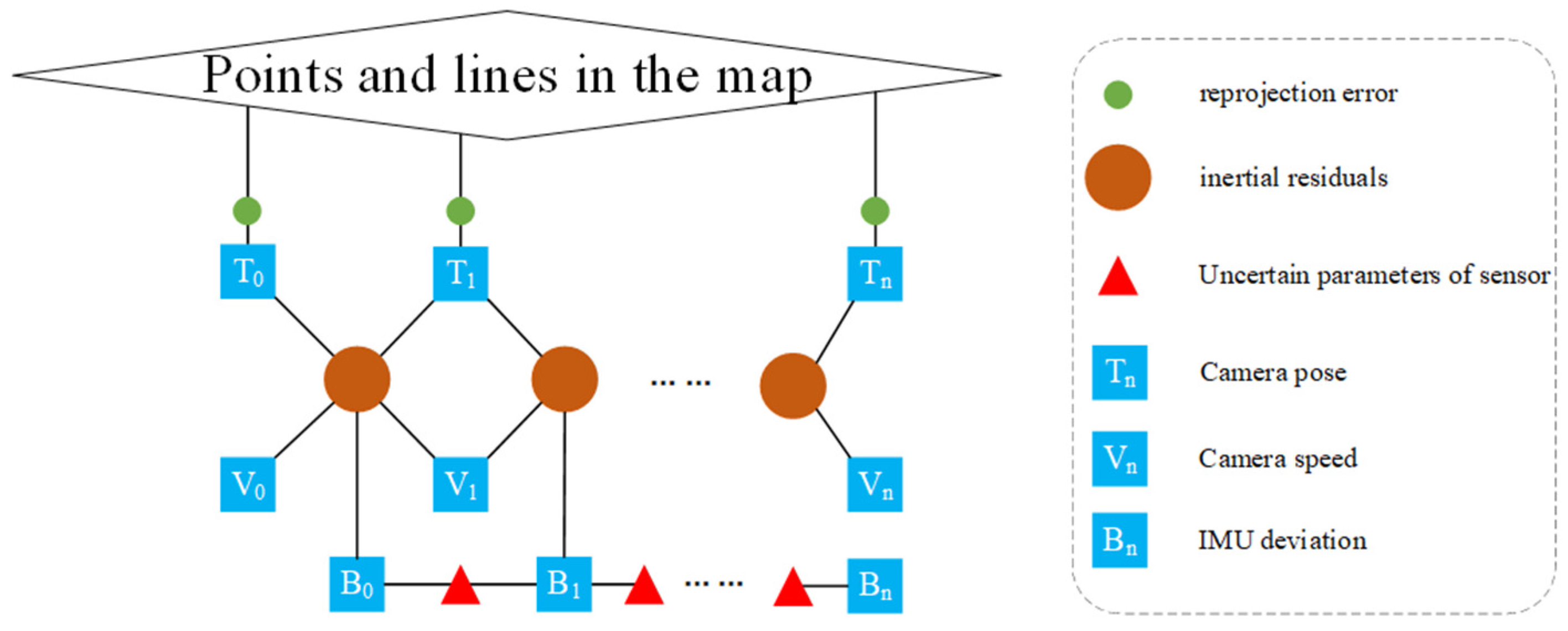
3.2. Visual-Inertia Initialization

In this section, the parameter and deviation of visual inertia are estimated by means of a step-by-step joint initialization method referring to the initialization method in ORB-SLAM3 [20]. Visual-inertial Bundle Adjustment (BA) optimization is first used to form an initial map consisting of multiple poses of camera and sparse point clouds. The camera pose R t was fixed in the map, and R t was used to calculate the IMU motion residual in the second stage.
In the inertia-only initialization stage, the goal is to obtain the best estimate of the inertia variable. Based on the maximum a posteriori estimation, only fixed camera trajectories and inertial variables between these keyframes are used. These inertial variables can be superimposed on the inertia-only state variable V k as shown in Equation (14):
V k = { U , g , , v ¯ 0 : k }
U is the scale factor in the pure visual initialization stage. g is the vector of gravity, is the accelerometer and gyro deviation assumed to be constant at initialization, v ¯ 0 : k is the scaled camera speed from the first key frame to the last key frame, which is initially estimated by means of a fixed camera trajectory.
Based on the above description, only the inertial measurement values are considered:
X 0 : k = ˙ { X 0 : 1 , X 0 : 2 , , X k 1 : k }
Therefore, the maximized posterior distribution is shown in Equation (16).
p ( V k X 0 : k ) p ( X 0 : k V k ) p ( V 0 )
where p ( X 0 : k l V k ) represents the likelihood value and p ( V 0 ) represents the prior value.
According to markov properties, image measurement at a certain moment only depends on the state at that moment. According to the standard independence assumption between measurements, Equation (16) can be expressed as Equation (17).
p ( V 0 ) Π p ( x i j s i , s j ) Π p ( Z i s i )
Considering the independence of measurement, the maximum posterior estimation problem of pure inertia can be expressed as Equation (18).
V k = arg max V k ( p ( V 0 ) i = 1 k p ( χ i 1 : i μ , g , , v ¯ i 1 , v ¯ i ) )
The maximum posteriori estimate V k corresponds to the maximum of Equation (17), or the minimum of the negative logarithmic posteriori estimate. The negative logarithm and Gaussian error are taken for the pre-integration and prior distribution of IMU. The negative logarithm posterior estimate can be written as the sum of squares of residuals. Finally, the optimization problem is obtained, as shown in Equation (19).
V k = arg min v k ( γ p 2 + i = 1 k γ ψ 1 , Σ 2 n 1 , )
The difference between the optimization equation of Equation (19) and Equation (14) is that it does not consider visual residual, but uses prior residual γ p to make IMU deviation close to zero, and the covariance of Equation (15) is given by IMU features.
After inertial optimization, frame pose and velocity, as well as 3D map points, are scaled to the estimated scale and rotated to align the Z axis with the estimated gravity vector. During this time, various biases will be updated and inertial measurement unit pre-integration will be repeated to reduce linearization errors. The parameter Formula (15) of IMU is obtained by comprehensive use of visual constraints and IMU constraints. After initialization, the detected new key points and new measurements of IMU can be used to locate and build maps.

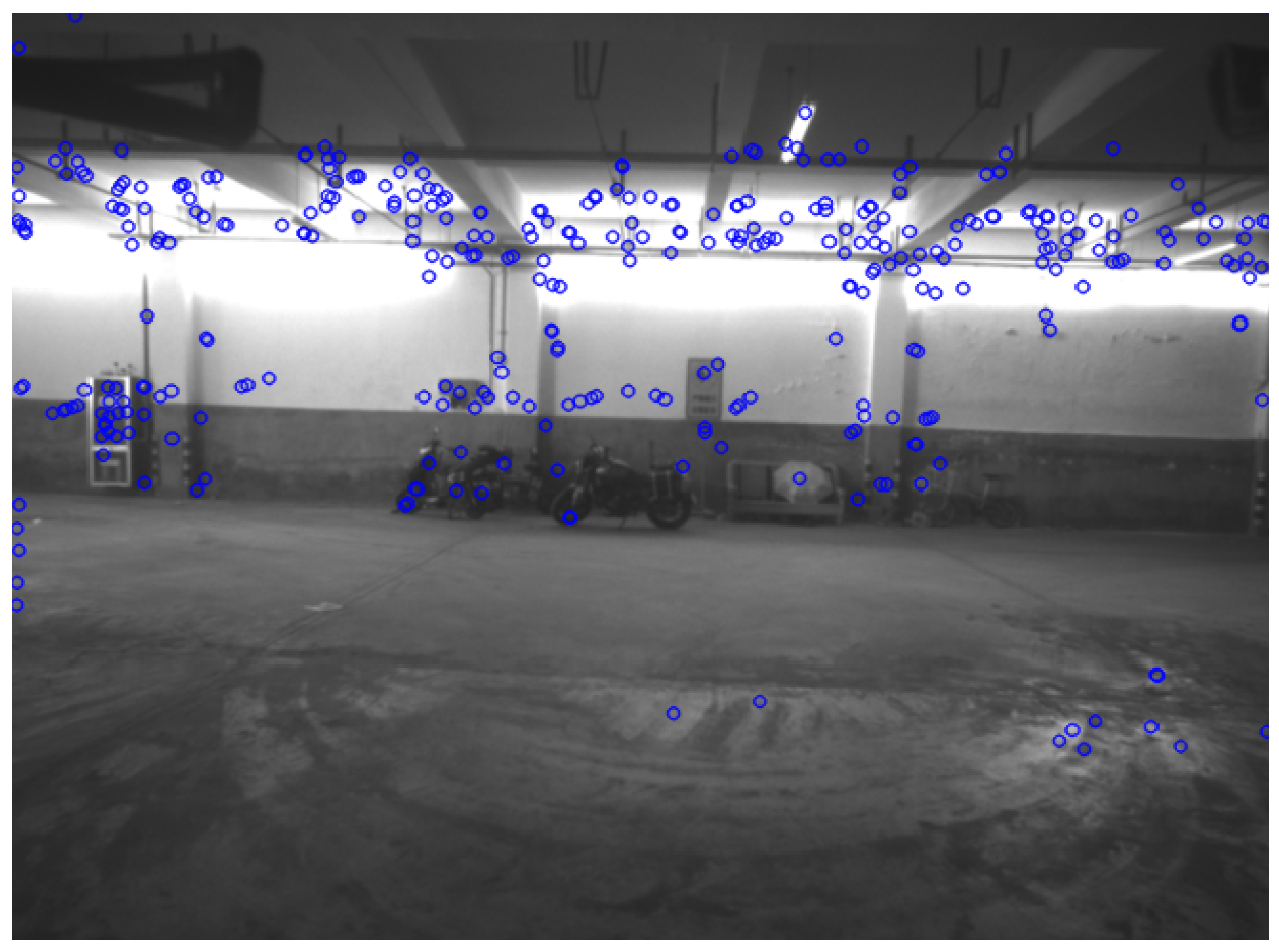
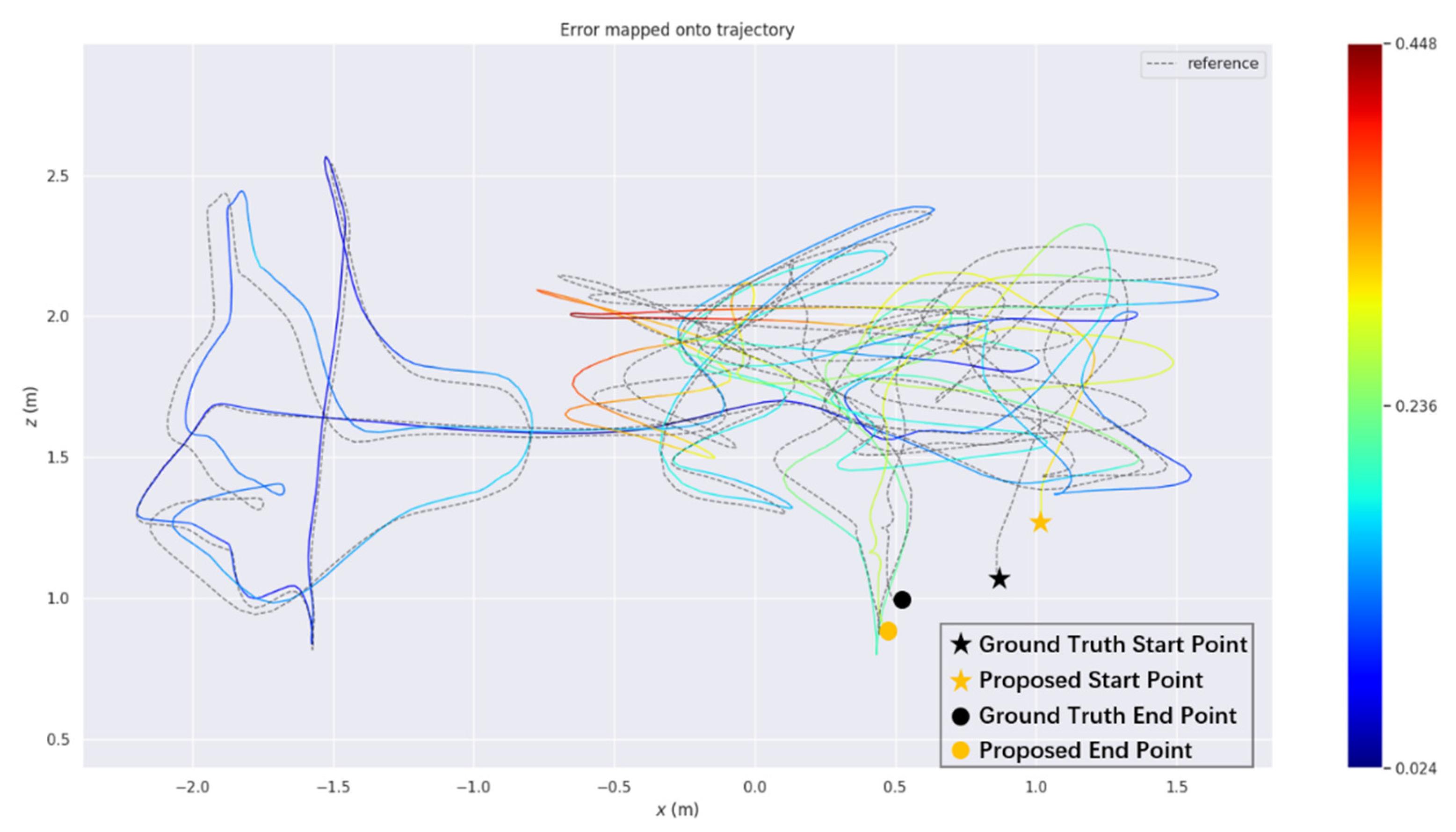
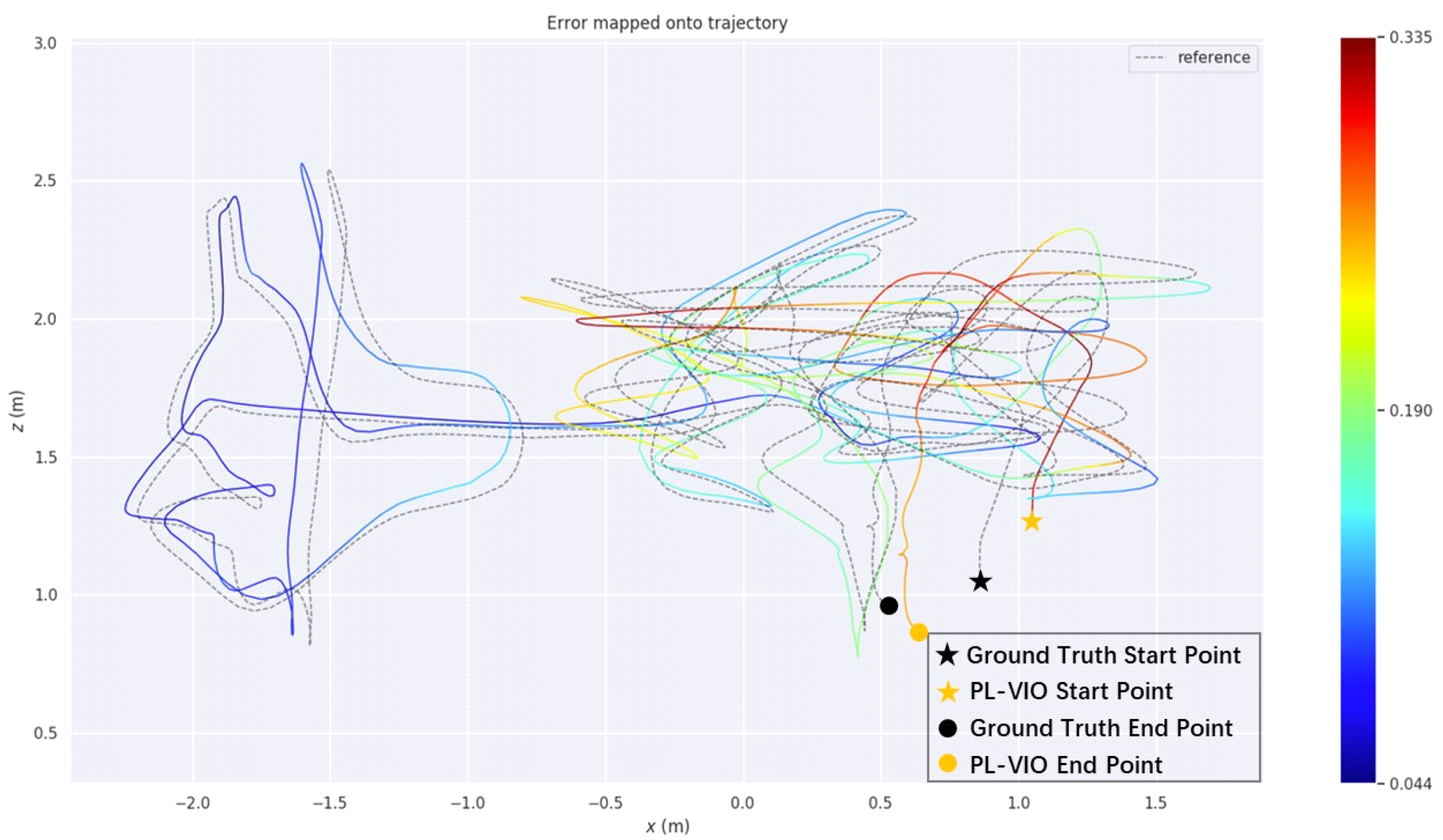
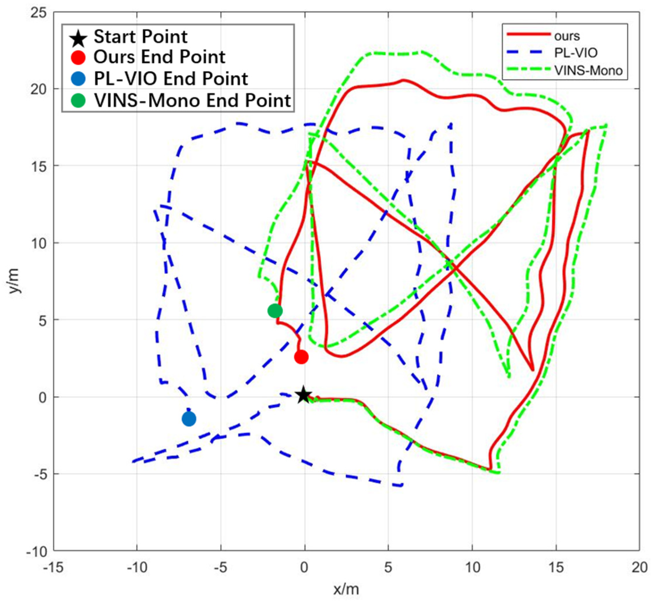
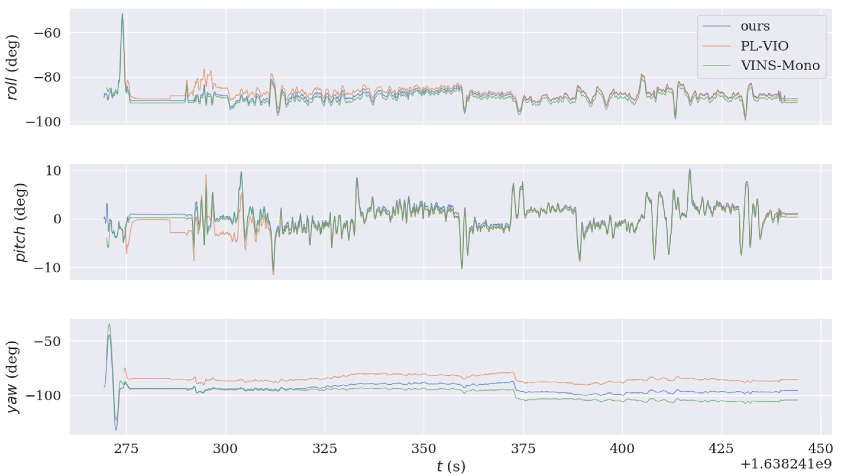
4. Experimental Results and Their Analysis

The experiments are accomplished with the DJI Manifold2-C computer, whose configuration is as follows: the CPU is the Intel® Core™ i7-8559U processor; the main frequency is between 2.7 GHz and 4.5 GHz; the memory is 8 G; the computer has no GPU; its system is Ubuntu 16.04 LTS 64 bits with ROS Kinetic. To evaluate the algorithm, we use the public dataset EuRoC [23], which contains 11 data sequences of the three grades: simple, medium and difficult. The comprehensive consideration of illumination, movement speed and other flight conditions can thoroughly evaluate the performances of the algorithm.
Figure 10 shows the average computation time per frame of each module under EuRoC data set of three algorithms.
It can be seen from Figure 10 that point feature extraction and matching takes 30 ms if SURF and FLANN algorithms are adopted, which has little impact on real-time performance of the system but has better positioning accuracy and stability (see Figures 13 and Figure 14). The average time consuming of the line feature extraction algorithm in this paper is 20 ms per frame, and the time consuming of point and line feature extraction and matching thread is 55 ms in total. The overall time consuming of the front end of the system is reduced and it can run in real time.
The motion estimation error of VINS-Mono, PL-VIO and the algorithm in this paper under the EuRoC data set (a total of 10 sub-sequences) is shown in Table 1, Absolute Trajectory error (ATE) is used to evaluate the accuracy of algorithms.
According to the alignment and pose error of the algorithm in data 3 in Table 1 under EuRoC data set, it can be concluded that the point-line features of MH_01_easy and V2_01_easy are sufficient, full of light and without fast motion. However, the advantages of this are mainly aimed at scenes with missing texture and fast movement, so the PL-VIO positioning accuracy in these two data sets is higher than that of the algorithm in this paper. The algorithm of this paper is optimal in all other scenes. In the MH_04_difficult sequence with missing scene texture and V1_03_difficult sequence with fast camera movement, the algorithm presented in this paper shows excellent accuracy.
In the scene in Figure 11, lighting changes dramatically, and objects with few features such as windows and door frames are all surrounded by them, and their motion is very violent, which belongs to one of the most extreme environments and is very consistent with the scene targeted in this paper, which puts forward high requirements for the algorithm.
In order to verify the positioning effect of the three algorithms in this scenario and make the results more convincing, the EVO (Evaluation of Odometry and SLAM) toolkit is used to draw the results.
Figure 12, Figure 13 and Figure 14 are the comparison diagrams of plane trajectory and real trajectory of VINS-Mono, PL-VIO and our algorithm under this data set, respectively.
Figure 12, Figure 13 and Figure 14 represent the Absolute Pose Error (APE) of the two sequences. The gradient color band from dark blue to red in the figure represents the Error size, and the values at the top and bottom of the color band are the maximum and minimum values of the Error. The closer the track color is to dark blue, the smaller the error between track and true value is. V1_03_difficult sequence is a data set of indoor motion and fuzzy illumination. Figure 11, Figure 12 and Figure 13 respectively show the comparison of plane trajectory and real trajectory of this algorithm and PL-VIO under this sequence. The absolute pose error of VINS-Mono, PL-VIO and our algorithm is 0.236 m, 0.190 m and 0.148 m respectively. It can be seen that the gap between the algorithm in this paper and the truth value is closer and the stability is higher.
The real-time error of the three algorithms in V1_03_difficult is shown in Figure 15.
Figure 15a shows the real-time absolute pose error. It can be seen that the trajectory of the proposed algorithm is smoother than that of the other two algorithms. Figure 15b shows the root mean square error, median error, mean error, extreme error and sum of squares of error of the three algorithms. The algorithm in this paper is optimal in all indicators.
As can be seen from Figure 16, the algorithm presented in this paper has concentrated error distribution, stable effect and strong robustness. Overall, the performance of the proposed algorithm is better than the other two algorithms.

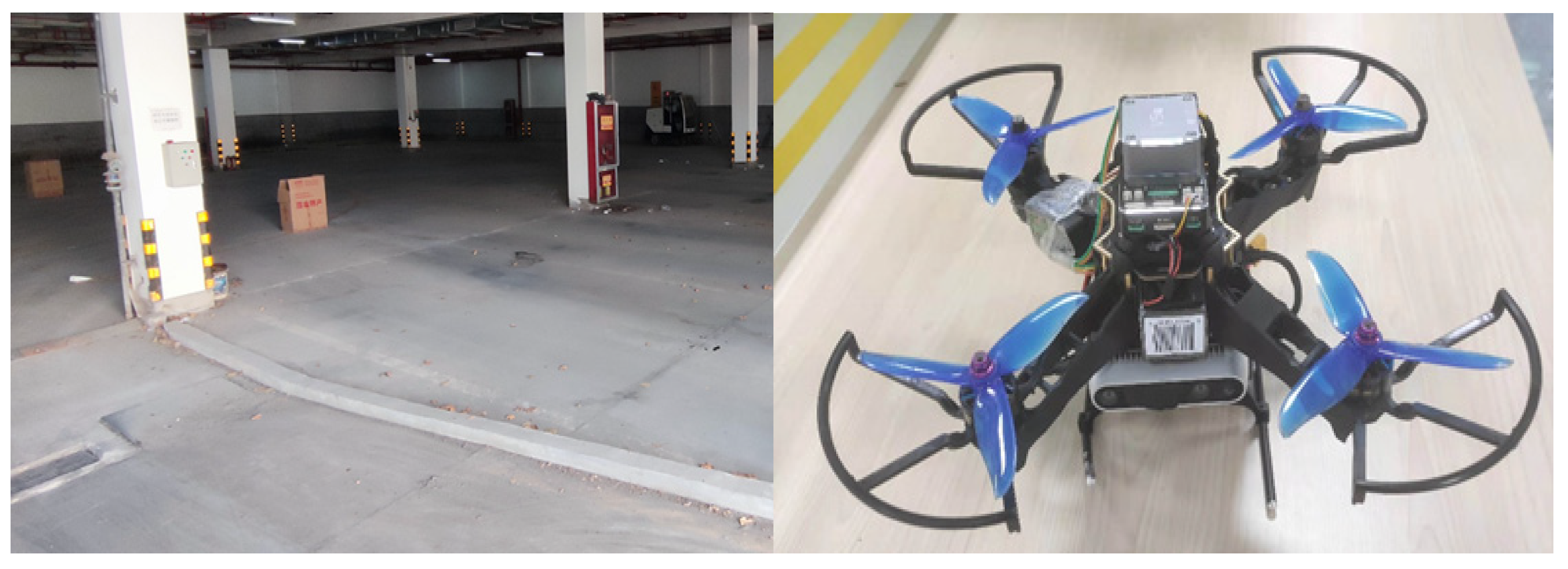
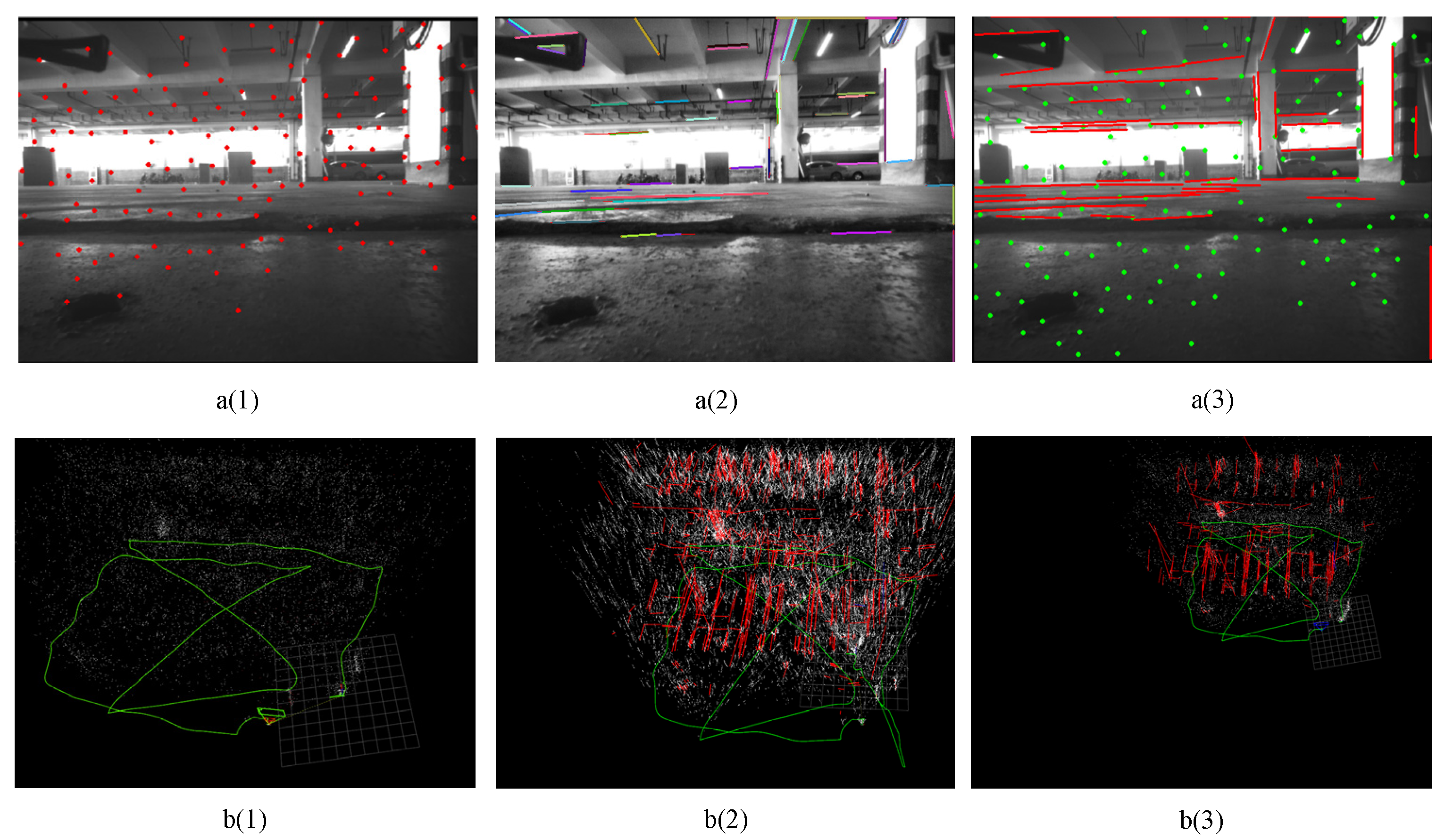
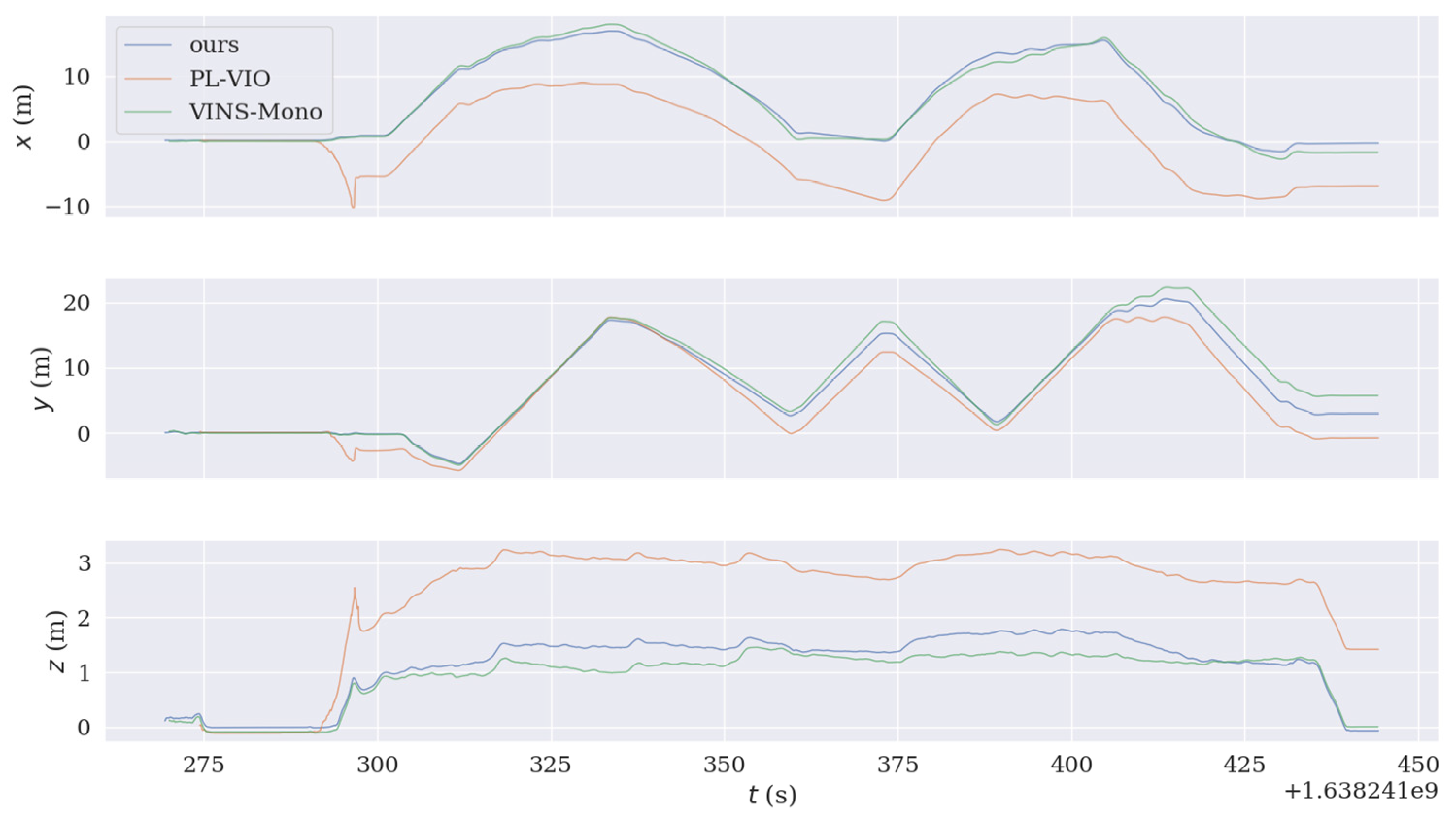
Actual Scene Experiment

The experimental site is the underground parking lot of Northwest China University of Technology. The test scene is relatively empty and surrounded by white walls, so it is difficult to extract point feature. The light intensity of different positions and the speed of UAV flight is not fixed, which is a challenge for the algorithm performance. To verify the performance of the algorithm in actual weak-textured environment, a quadrotor drone is equipped with a smart computing host and a D453i camera (camera frame rate 30 Hz, IMU frame rate 200 Hz). The three algorithms were tested online. The experimental field and the experimental acquisition equipment are shown in Figure 17.
Experimental scheme is as belows. After starting the positioning algorithm, the UAV is controlled to fly for a period of time. The landing point coincides with the starting point, locate and map its trajectory in real time, and compare the distance between the final plane and the origin after the landing of the three algorithms.
As shown in a(1), a(2) and a(3) in Figure 18, compared with the VINS-Mono algorithm, the PL-VIO algorithm and the algorithm in this paper can extract more line features in an open environment with more white walls and insufficient point feature extraction. It can be seen from b(1) and b(2) that after the algorithm in this paper removes mismatching and redundant line features, the number of remaining line segments is smaller, but the quality is higher, which can reduce the mismatching rate of line features.
The actual running trajectories of the three algorithms are shown in Figure 19.
After running, the distance from the origin of our algorithm, PL-VIO and VINS-Mono are 2.902 m, 6.99 m and 5.963 m respectively. By comparison, the error of the proposed algorithm in practical scenarios is smaller, and the accuracy of the proposed algorithm is 51.33% higher than that of the VINS-Mono algorithm and 58% higher than that of the PL-VIO algorithm.
Based on Figure 19, it can be seen that the positioning results of the PL-VIO system began to drift after the aircraft took off, because the SLAM system with line features could not calculate all the initialization parameters within a short time after startup. After running for a while, the system stabilizes as new features are added. The algorithm in this paper optimizes image processing and initialization, so that the system can calculate accurate initialization parameters in a short time. Therefore, the trajectory of UAV is stable and the positioning accuracy is relatively high after startup. Although VINS-Mono does not diverge, its positioning accuracy is not as high as that of the proposed algorithm.
Figure 20 and Figure 21 record the pose changes of the three systems after initialization.
By comparing Figure 20 and Figure 21 respectively, it can be seen that our algorithm has shorter initialization time and smoother trajectory compared with VINS-Mono and PL-VIO.
Through the experimental comparison, it can be found that the proposed algorithm can better solve the pose estimation problem in the low texture region and provide better initialization effect and feature extraction matching effect of SLAM system, which has the best performance in the actual scene. Due to the fusion of line features and IMU data, the accuracy and robustness of the algorithm are improved effectively.

5. Conclusions

In this paper, a novel point-line visual inertial SLAM method is proposed. Public data set EuRoC and UAV flight tests are used for validation. The conclusions are as follows:
(1)
Adding bilateral filtering algorithm to SLAM front-end image preprocessing module can effectively reduce image noise and the difficulty of point-line feature extraction.
(2)
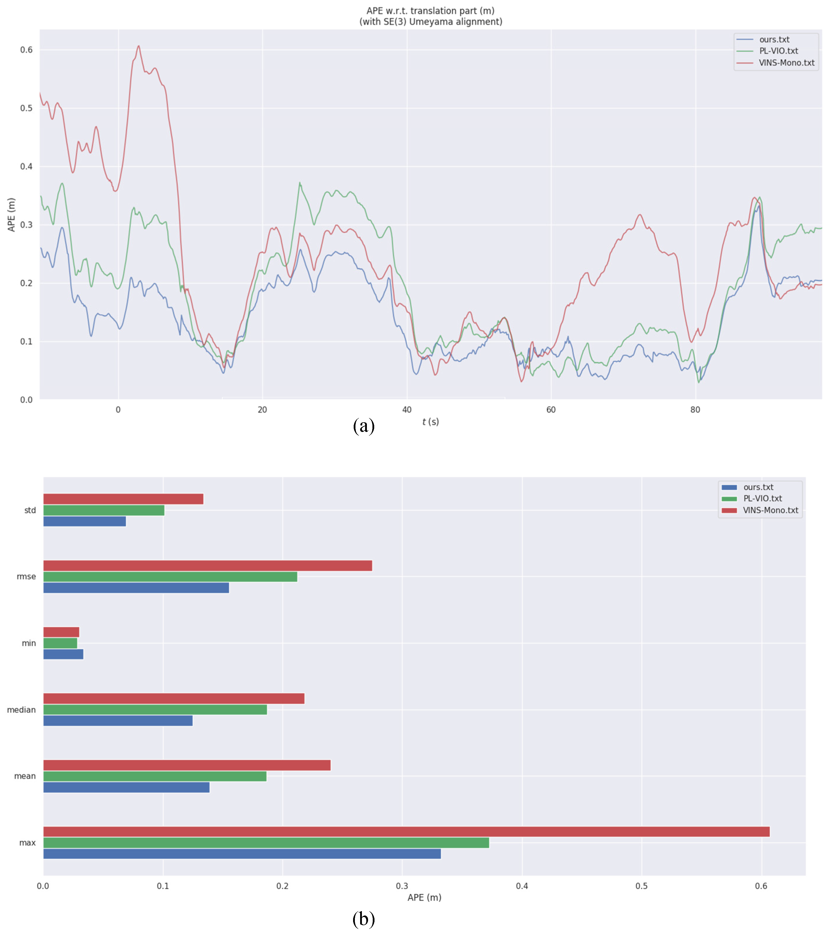
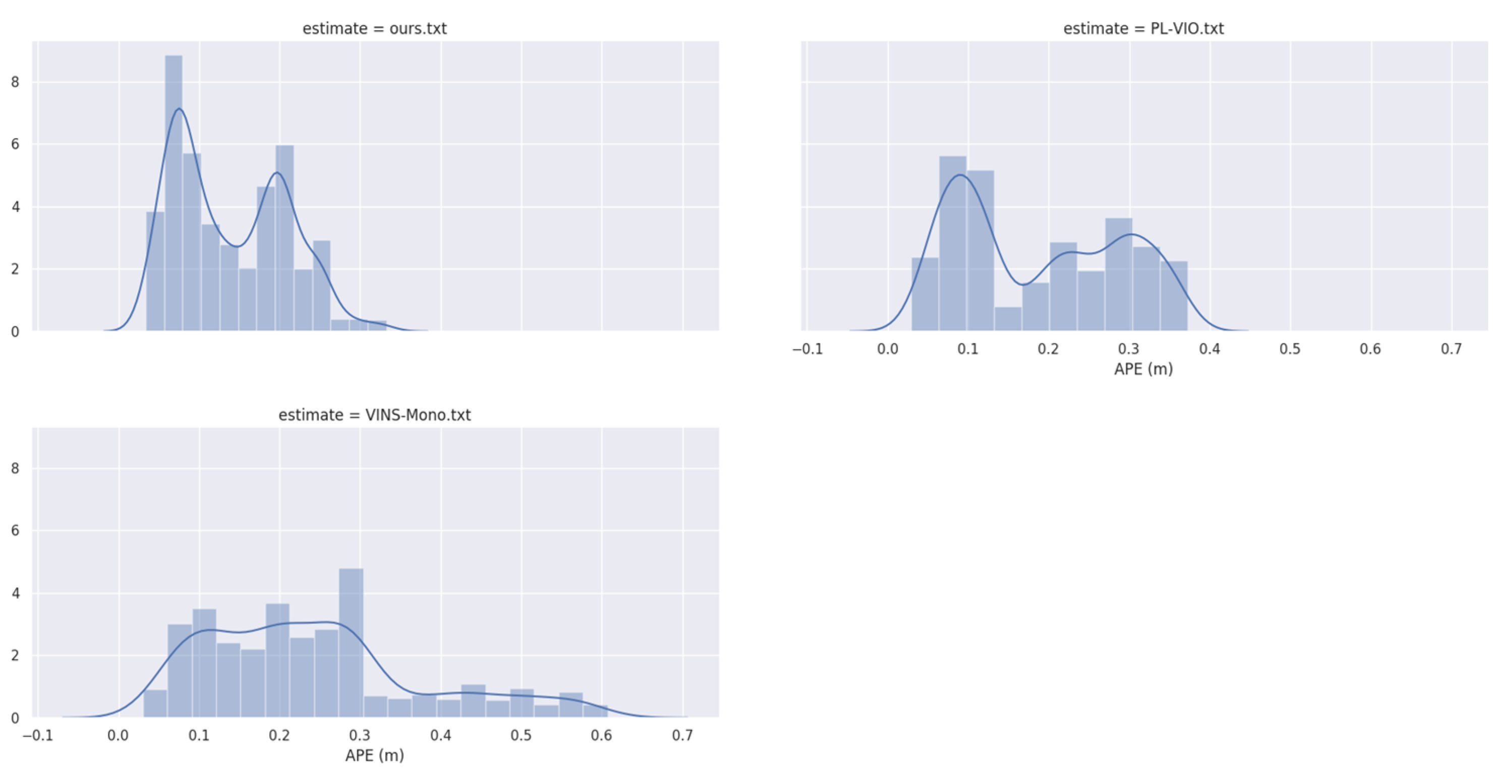
Aiming at the problem of image blur when the camera moves, SURF algorithm and FLANN matching algorithm are adopted. Although the overall consumption time of processing point features is slightly increased, the positioning accuracy is significantly improved.
(3)
The parameters of LSD line feature extraction algorithm are selected, and the extraction speed is increased by 3 times by using length suppression strategy line feature. A line feature matching method based on geometric constraints is proposed, and the matching time of line segments is reduced by 66.66%.
(4)
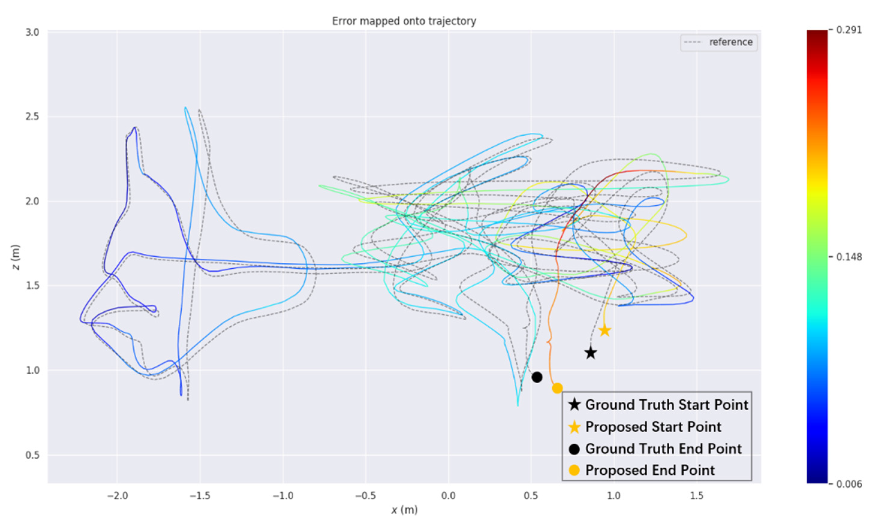
The step joint initialization method greatly reduces the initialization time, improves accuracy and makes the location trajectory smoother.

Author Contributions

Writing—Review & Editing, T.Z.; Writing—Original Draft Preparation, C.L.; Validation, J.L.; Methodology, M.P.; Project administration, M.W. All authors have read and agreed to the published version of the manuscript.

Funding

This research was funded by National Natural Science Foundation of China (NSFC) (61603297) and Natural Science Foundation of Shaanxi Province (2020JQ-219).

Institutional Review Board Statement

The paper does not involve any ethical guidelines.

Data Availability Statement

Publicly available datasets were analyzed in this study. This data can be found here: https://github.com/topics/euroc-dataset (accessed on 13 December 2021).

Acknowledgments

The authors wish to express their appreciation to the National Natural Science Foundation of China (NSFC) (61603297) and Natural Science Foundation of Shaanxi Province (2020JQ-219).

Conflicts of Interest

The authors declare no conflict of interest.

References

  1. Latif, Y.; Doan, A.D.; Chin, T.J.; Reid, I. Sprint: Subgraph place recognition for intelligent transportation. In Proceedings of the IEEE International Conference on Robotics and Automation (ICRA), Paris, France, 31 May–31 August 2020; pp. 5408–5414. [Google Scholar]
  2. Bryson, M.; Sukkarieh, S. Building a Robust Implementation of Bearing-only Inertial SLAM for a UAV. J.-Ournal Field Robot. 2010, 24, 113–143. [Google Scholar] [CrossRef] [Green Version]
  3. Geneva, P.; Eckenhoff, K.; Huang, G. A Linear-Complexity EKF for Visual-Inertial Navigation with Loop Clo-sures. In Proceedings of the International Conference on Robotics and Automation (ICRA), Montreal, QC, Canada, 20–24 May 2019. [Google Scholar]
  4. 4. Qin, T.; Li, P.; Shen, S. VINS-Mono: A Robust and Versatile Monocular Visual-Inertial State Estimator. IEEE Trans. Robot. 2018, 34, 1004–1020. [Google Scholar] [CrossRef] [Green Version]
  5. Mur-Artal, R.; Tardós, J.D. ORB-SLAM2: An Open-Source SLAM System for Monocular, Stereo, and RGB-D Cameras. IEEE Trans. Robot. 2016, 33, 1255–1262. [Google Scholar] [CrossRef] [Green Version]
  6. Burdziakowski, P. Towards precise visual navigation and direct georeferencing for MAV using ORB-SLAM2. In Proceedings of the Baltic Geodetic Congress (BGC Geomatics), Gdansk, Poland, 22–25 June 2017; pp. 394–398. [Google Scholar]
  7. Aguilar, W.G.; Rodríguez, G.A.; Álvarez, L.; Sandoval, S.; Quisaguano, F.J.; Limaico, A. Visual SLAM with a RGB-D camera on a quadrotor UAV using on-board processing. In International Work-Conference on Artificial Neural Networks; Springer: Cham, Switzerland, 2017; pp. 596–606. [Google Scholar]
  8. Lowe, D. Distinctive image features from scale-invariant key points. Int. J. Comput. Vis. 2003, 20, 91–110. [Google Scholar]
  9. Rosten, E.; Drummond, T. Machine Learning for High-Speed Corner Detection. In Proceedings of the European Conference on Computer Vision, Graz, Austria, 7–13 May 2006; Springer: Berlin/Heidelberg, Germany, 2006; pp. 430–443. [Google Scholar]
  10. Rublee, E.; Rabaud, V.; Konolige, K.; Bradski, G. ORB: An efficient alternative to SIFT or SURF. In Proceedings of the International conference on computer vision, Barcelona, Spain, 6–13 November 2011; pp. 2564–2571. [Google Scholar]
  11. Vakhitov, A.; Funke, J.; Moreno-Noguer, F. Accurate and Linear Time Pose Estimation from Points and Lines. In Proceedings of the European Conference on Computer Vision, Graz, Austria, 7–13 May 2006; Springer: Cham, Switzerland, 2016; pp. 583–599. [Google Scholar]
  12. Zuo, X.; Xie, X.; Liu, Y.; Huang, G. Robust Visual SLAM with point and line features. In Proceedings of the IEEE/RSJ International Conference on Intelligent Robots and Systems (IROS), Vancouver, BC, Canada, 24–28 September 2017; pp. 1775–1782. [Google Scholar]
  13. Pumarola, A.; Vakhitov, A.; Agudo, A.; Sanfeliu, A.; Moreno-Noguer, F. PL-SLAM: Real-time monocular visual SLAM with points and lines. In Proceedings of the IEEE international conference on robotics and automation (ICRA), Singapore, 29 May–3 June 2017; pp. 4503–4508. [Google Scholar]
  14. Gomez-Ojeda, R.; Moreno, F.A.; Zuniga-Noël, D.; Scaramuzza, D.; Gonzalez-Jimenez, J. PL-SLAM: A stereo SLAM system through the combination of points and line segments. IEEE Trans. Robot. 2019, 35, 734–746. [Google Scholar] [CrossRef] [Green Version]
  15. He, Y.; Zhao, J.; Guo, Y.; He, W.; Yuan, K. Pl-VIO: Tightly-coupled monocular visual–inertial odometry using point and line features. Sensors 2018, 18, 1159. [Google Scholar] [CrossRef] [PubMed] [Green Version]
  16. Wen, H.; Tian, J.; Li, D. PLS-VIO: Stereo Vision-inertial Odometry Based on Point and Line Features. In Proceedings of the IEEE International Conference on High Performance Big Data and Intelligent Systems (HPBD&IS), Vientiane, Laos, 23–23 May 2020; pp. 1–7. [Google Scholar]
  17. Fu, Q.; Wang, J.; Yu, H.; Ali, I.; Guo, F.; He, Y.; Zhang, H. PL-VINS: Real-Time Monocular Visual-Inertial SLAM with Point and Line. arXiv 2020, arXiv:2009.07462. [Google Scholar]
  18. Tomasi, C.; Manduchi, R. Bilateral filtering for gray and color images. In Proceedings of the IEEE Sixth International Conference on Computer Vision, Bombay, India, 4–7 January 1998; pp. 839–846. [Google Scholar]
  19. Von Gioi, R.G.; Jakubowicz, J.; Morel, J.M.; Randall, G. LSD: A fast line segment detector with a false detection co-ntrol. IEEE Trans. Pattern Anal. Mach. Intell. 2008, 32, 722–732. [Google Scholar] [CrossRef] [PubMed]
  20. Muja, M.; Lowe, D.G. Fast Approximate Nearest Neighbors with Automatic Algorithm Configuration. In Proceedings of the International Conference on Computer Vision Theory & Application Vissapp, Lisboa, Portugal, 5–8 February 2009; Volume 2, pp. 331–340. [Google Scholar]
  21. Campos, C.; Elvira, R.; Rodríguez, J.J.G.; Montiel, J.M.M.; Tardós, J.D. ORB-SLAM3: An Accurate Open-Source Library for Visual, Visual–Inertial, and Multimap SLAM. IEEE Trans. Robot. 2021, 37, 1874–1890. [Google Scholar] [CrossRef]
  22. Chaudhury, K.N.; Sage, D.; Unser, M. Fast O (1) bilateral filtering using trigonometric range kernels. IEEE Trans. Image Process. 2011, 20, 3376. [Google Scholar] [CrossRef] [PubMed] [Green Version]
  23. Burri, M.; Nikolic, J.; Gohl, P.; Schneider, T.; Rehder, J.; Omari, S.; Achtelik, M.W.; Siegwart, R. The EuRoC micro aerial vehicle datasets. Int. J. Robot. Res. 2016, 35, 1157–1163. [Google Scholar] [CrossRef]
Figure 1. The algorithm framework.
Drones 06 00023 g001
Figure 2. Point line feature processing flow chart.
Drones 06 00023 g002
Figure 3. Box filter image processing template.
Drones 06 00023 g003
Figure 4. SURF feature extraction before bilateral filtering.
Drones 06 00023 g004
Figure 5. SURF feature extraction after bilateral filtering.
Drones 06 00023 g005
Figure 6. SURF is matched with the original algorithm.
Drones 06 00023 g006
Figure 7. FLANN algorithm matching.
Drones 06 00023 g007
Figure 8. Line segment geometric constraint matching.
Drones 06 00023 g008
Figure 9. Visual-Inertial initialization.
Drones 06 00023 g009
Figure 10. Consumption time of the front-end algorithm.
Drones 06 00023 g010
Figure 11. V1_03_difficult data scenario [23].
Drones 06 00023 g011
Figure 12. The VINS-Mono shows the absolute position error in the V1_03_difficult plane.
Drones 06 00023 g012
Figure 13. The P L-VIO shows the absolute position error in the V1_03_difficult plane.
Drones 06 00023 g013
Figure 14. The proposed shows the absolute pose error in the V1_03_difficult plane.
Drones 06 00023 g014
Figure 15. The real-time errors of the three algorithms in V1_03_difficult. (a) the real-time absolute pose error in V1_03_difficult. (b) shows the root mean square error, median error, mean error, extreme error and sum of squares of error of the three algorithms.
Drones 06 00023 g015
Figure 16. Range of absolute pose error distribution in V1_03_difficult.
Drones 06 00023 g016
Figure 17. Experimental field and equipment.
Drones 06 00023 g017
Figure 18. Actual scene experiment. a(1) VINS-Mono algorithm for feature extraction of images in real scenes. a(2) PL-VIO algorithm for feature extraction of images in real scenes. a(3) The proposed algorithm for feature extraction of images in real scenes. b(1) The real-time localization trajectory of VINS-Mono algorithm is in the actual scene. b(2) The real-time localization trajectory of PL-VIO algorithm is in the actual scene. b(3) The real-time localization trajectory of the proposed algorithm is in the actual scene.
Drones 06 00023 g018
Figure 19. Plar trajectories of the three algorithms in the actual scenario.
Drones 06 00023 g019
Figure 20. The displacement of the three algorithms on the X, Y and Z axes respectively.
Drones 06 00023 g020
Figure 21. The attitude Angle changes of three algorithms.
Drones 06 00023 g021
Table 1. Motion estimation errors of three algorithms in the EuRoC dataset (RMSE unit: m) Absolute trajectory error for both algorithms.
SerialVINS-MonoPL-VIOOurs
MH_01_easy0.3550.1290.145
MH_02_easy0.3430.1830.150
MH_03_medium0.5580.2620.218
MH_04_difficult0.5950.3770.224
MH_05_difficult0.5870.2830.257
V1_01_easy0.3590.1660.085
V1_03_difficult0.5290.2210.148
V2_01_easy0.2800.1090.128
V2_02_medium0.5460.1740.150
V2_03_difficult0.5720.3190.183
Publisher’s Note: MDPI stays neutral with regard to jurisdictional claims in published maps and institutional affiliations.

