1. Introduction
Machine-type communications have witnessed a renewed interest from the scientific community thanks to advancements in technology and the plethora of new applications involving them. Statistical reports already proved a steady increase in the number of machine-type or Internet of Things (IoT) links (see, e.g.,
https://www.statista.com/statistics/802690/worldwide-connected-devices-by-access-technology/ or
https://www.ericsson.com/en/mobility-report/reports/november-2019/iot-connections-outlook, accessed on 7 September 2021.), but the massive presence of IoT devices might not be the only major challenge to be addressed for the future. Other key challenges lie on the more differentiated and stringent requirements on communication performance—the demand—imposed by the several applications and use cases possible. These may include autonomous vehicles, wearables, industrial IoT for Industry 4.0, data monitoring, alarm detection, municipality services and many others, in which one can observe that commonalities are few. These aspects call for new paradigms to network design. To avoid the densification and deployment of new terrestrial bases needing huge investments in capital and operational expenditures, a viable and largely foreseen solution can be found in mobile base stations (BSs).
Unmmaned aerial vehicles (UAVs) (a.k.a. drones), where mobile BSs can be mounted, represent very interesting means to add the required flexibility and scalability for the future networks. UAVs have, in fact, the potential to fly on-demand and exactly where is needed. Moreover, they are not tied to roads, not affected by traffic congestion and can feature good connectivity with both on-ground users and terrestrial BSs (i.e., backhaul), thanks to the large probability of being in the line of sight (LoS). The usage of UAVs as mobile BSs is especially suited for massive machine-type communication (mMTC) and IoT links, since IoT nodes are mostly static (do not change their position over time) and their traffic demand is usually predictable [
1]. The knowledge of these two basic inputs allows to make decisions in advance on the trajectory to follow to maximize IoT service, plan periodical flights when the demand arises, modify the UAV behaviour if needed, and so on. This may be further relevant if these mobile BSs have to direct themselves in remote and different areas where the nodes are placed. To consider at our best a scenario with the plurality of IoT applications mentioned before, as pictured in
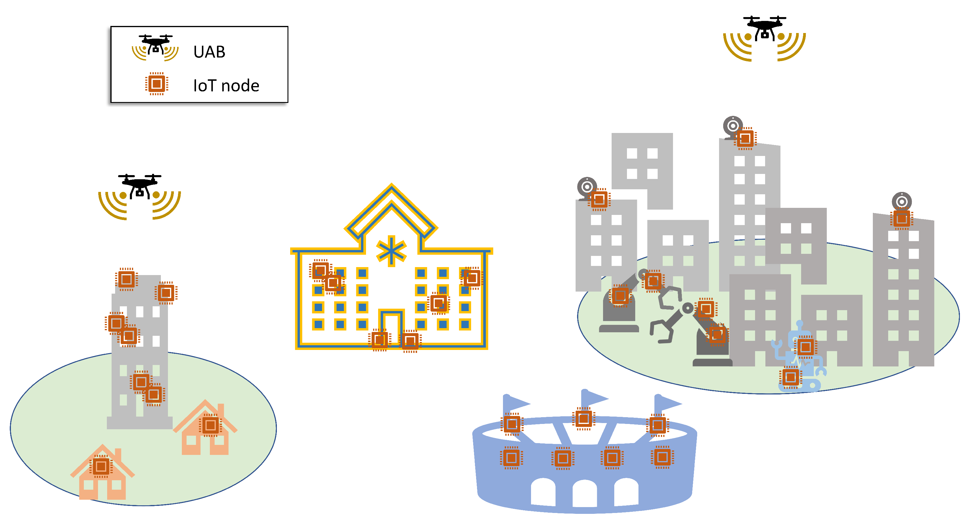
Figure 1, we consider a massive number of IoT devices scattered in different zones of a service area, requesting to transmit a periodical packet. This is a realistic scenario, and perfect for UAV services during a single flight.
Thanks to their versatility, flying network nodes like UAVs have gained an ever-increasing interest from researchers concerning standardization bodies. The 3rd Generation Partnership Project (3GPP), after considering the feasibility of UAVs being user equipment (UE) (i.e., end users of the cellular network), started approaching on-board radio access for UAVs (denoted with the acronym UxNB) at the beginning of Rel. 17 [
2,
3]. Because of the several activities considering the aid of UAVs to cellular users, we focus on the cellular radio access technology, as stated in the 3GPP documents [
4]. In fact, if a UAV could have installed the same radio-frequency equipment with a similar protocol stack to target both IoT nodes and broadband users, it would be convenient for mobile operators. To this purpose, there exist a number of technologies targeting IoT applications which follow the fourth-generation (4G) numerology [
5]. In particular, we will focus on NarrowBand-IoT (NB-IoT) for the design intended to target low-end IoT applications with low data rates, delay tolerance, massive connections, and extremely wide coverage [
6]. To this end, this work can be considered an extension of [
1], where an initial and simple approach was proposed to UAV-aided NB-IoT networks.
In this article, we throroughly study different approaches to aerial support for NB-IoT networks, in order to provide a general overview of the challenges and potentials of these systems. To properly assess the network performance of UAVs serving NB-IoT nodes, we jointly consider as performance metrics the percentage of completely served nodes, the throughput provided and the latency which has to be expected and the IoT nodes’ energy consumption. Our key contributions can be summarized as follows:
We propose a UAV-aided NB-IoT scenario with several hundreds of nodes, located in different parts of the area as to simulate diverse applications. Differently from other papers in literature, the NB-IoT technology is considered in details as specified by the 3GPP documents and studied in all of its features, including the signaling procedures and the parameters’ implications of the three NB-IoT coverage classes;
we investigate the performance in terms of number of completely served nodes, achieved network throughput, perceived latency and energy consumption of nodes;
we analyze the impact of using different UAV trajectories and the effect of varying UAV parameters, such as speed and height.
The article is organized as follows. In
Section 2, we give an overview of the literature about UAV-aided networks in IoT applications. NB-IoT and its features are presented in
Section 3.
Section 4 describes the scenario and the network model. Final simulation results are reported and discussed in
Section 5. Finally,
Section 6 concludes the article.
2. Literature Overview
Initial studies on UAV-aided networks focused on the key link-level considerations, and specifically on the characterization of path loss and its impact on the so-called air-to-ground (ATG) channel [
7,
8]. These activities on UABs were followed by the aim of finding an acceptable trade-off between coverage, capacity and connectivity, as in [
9]. To be more specific, in [
8] the effect of the user-UAV incident angle w.r.t. the ground plane as a function of drone height is studied. It is defined as elevation angle, and its aperture may determine a link being or not being free from obstructions and in LoS conditions. In the remainder of this article, we refer to the authors’ ATG model. In recent years, the interest in UAV-aided networking gradually increased, introducing studies ranging from UAV deployment issues to grant adequate coverage [
10,
11] to more complex problems of UAV trajectory design for fair and satisfactory quality of service to ground users [
12,
13,
14]. Differently from our objective, the majority of papers addresses a general user or device, forgetting the implications and limitations of the specific protocol procedures. For example. dynamic trajectories for the 3D space are studied in [
12] with the purpose to connect IoT nodes at their activation time. The authors jointly optimize the transmission power of ground nodes, the overall energy spent in movement and the choice of the next stop of each UAV. Some activities deal with the definition of an optimal trajectory for UABs. In [
13,
14] the trajectory is optimized with the aim of maximizing the minimum user rate. Optimization algorithms have also been studied for UAV placement to achieve optimal energy efficiency [
15,
16] by minimizing power consumption and transmission delays, which are interesting requirements for IoT applications. However, they do not consider specific protocol constraints or overhead as it is in 3GPP standards.
Similarly to this study, some other works related to UAVs are targeting the IoT field. As for recent examples, references [
17,
18] employ UAVs to gather IoT data from remote areas in which devices experience low connectivity or capacity issues. In [
17], the authors address the trajectory and resource allocation optimization for time-constrained IoT nodes, while the authors in [
18] optimize the UAB 3D placement and resource allocation minimizing the total transmission power of IoT devices and balancing the multi-UABs’ tasks. Reference [
19] focuses on the modelling and optimization of the carrier sensing-based medium access control (MAC) layer protocol of UAV-aided IoT networks; this paper analyses the achievable throughput as the performance metric and CSMA/CA as the MAC protocol. Moreover, reference [
20] studies different mechanism for the energy and delay aware task assignment of UAVs with onboard IoT nodes. More specific to the technology investigated hereby, reference [
21] studies trajectories for energy minimization in a NB-IoT context, reference [
22] investigates connectivity strategies for a specific NB-IoT application, and [
23] introduces a coverage analysis for UAV-aided NB-IoT networks. The NB-IoT protocol is considered in these articles, too, since it belongs to the machine-type emerging technologies [
6] and targets low data rates, delay tolerance, massive connections, and extremely wide coverage [
24]. However, these works usually lack either a fine-grained protocol study or focus on the optimization of one metric above the others. On the contrary, we aim at providing a more general overview of potentials and challenges of UAV-aided NB-IoT networks, with a deeper focus on protocol details rather than the optimization of a single performance metric. Moreover, optimization frameworks struggle to handle large input instances (e.g., a massive number of nodes in the scenario) because of the excessive computation times, in terms of days or weeks. For example, references [
13,
14] consider less than 10 users in the service area. Furthermore, in [
25], it is optimized the 3D locations of UAVs for wireless powered NB-IoT. Another work worth to mention is [
26]. The authors propose a NB-IoT model to collect underground soil parameters in potato crops using a UAV-aided network. The analysis in this case is mostly application-dependent, and therefore differs from our general evaluation with different metrics.
This activity can be considered an extension of [
1]. To the best of the authors’ knowledge, the literature still lacks the detailed model and protocol analysis of similar scenarios and setups. Therefore, the focus of this work is to extend and further discuss the system dynamics of NB-IoT networks served by an UAV, rather than compare our approach with other research activities. This study helps us to extract the major impacts of the overall protocol stack of the NB-IoT technology on UAV-aided networks.
3. The Narrowband-IoT Technology
The NB-IoT technology is intended to address the needs of mMTC, and has been standardized by 3GPP initially on Rel. 13 in 2016, with new functionalities introduced in the subsequent releases. It will be briefly described in this section, taking as references [
5,
27]. Particular emphasis is given to the uplink, which is the scenario of interest for this paper. The NB-IoT technical solution originates from the Long Term Evolution (LTE) technology, which has been substantially simplified to reduce the overheads, minimizing complexity, cost and consumption, and, at the same time, it keeps its usual mechanisms, such as synchronization, radio access and resource assignment. In addition, the NB-IoT technology features substantial flexibility allowing to deploy NB-IoTs cells by running a software update on already existing LTE cells. Indeed, three deployment options are available: Standalone, to reuse 200 kHz GSM carriers; guard-band, to exploit the guard band of two adjacent LTE carriers; and in-band, where one LTE Physical Resource Block (PRB) is reserved for NB-IoT within an LTE carrier bigger than 1.4 MHz. NB-IoT implements several mMTC-oriented enhancements, such as narrowband transmission and enhanced power saving techniques to increase battery life of UEs. In addition, up to 2048 and 128 repetitions in DL and UL, respectively, can be used to exploit the time variation of the radio channel, so that each replica can be decoded separately, or multiple replicas can be combined to further increase the reception probability. Furthermore, NB-IoT’s coverage enhancement is provided by defining three coverage classes: Normal, robust, and extreme. Classes are differentiated through thresholds based on Reference Signals Received Power (RSRP), defined to introduce three levels of coverage extension. Such thresholds depend on the cell deployment, the propagation environment (i.e., outdoor, indoor, deep-indoor, underground), and the spatial distribution of devices. Network parameters as the number of repetitions can be tuned separately for each class.
Before Rel. 15 introducing time division duplex (TDD) operation mode, the frequency division duplex (FDD) mode was the only option for NB-IoT. In this paper we consider the latter, since it is the primary mode used in most commercial networks and enables the maximum performance. The FDD mode implies different frequency bands to be used for UL and DL transmissions. The channel bandwidth of NB-IoT is 180 kHz, that corresponds to one LTE PRB. In UL, subcarrier spacing of either 15 or 3.75 kHz are possible, thus providing either 12 or 48 possible subcarriers within a 180 kHz resource block. The 15 kHz spacing allows transmission of either single or multitone (over up to 12 carriers) signals, while only single-carrier transmissions are possible for 3.75 kHz grid. On the contrary, in DL, only the 15 kHz resource grid is used.
3.1. Random Access Procedure
The random access (RA) procedure of a NB-IoT UE, which is necessary to allow an uplink packet transmission, is composed of multiple steps. To start with, the UE scans the channels for the synchronization signals. When it gets correctly synchronized to the base station, the UE obtains first the Master and then a number of Secondary Information Blocks (MIB and SIBs, respectively), containing all the relevant information about the network, the cell and its resource allocations. Then, to connect to the cell, the RA procedure starts by sending a preamble (or Msg1) during one of the periodic random access windows (NPRACH). After sending Msg1, the UE waits for Msg2 from the eNB. Note that, at this stage, the network is not aware of possible overlapping among UEs’ transmissions, which may happen if more than one UE chooses the same random preamble. With Msg2, the eNB notifies that it has received the specific preamble sequence and allocates NPUSCH resources for Msg3 for UEs which transmitted that specific sequence. In Msg3, each of the UEs sends different ID data and, in this case, collisions may actually happen, since UEs which used the same preamble sequence will use the same resources to send their Msg3. If the eNB can correctly receive at least one of the Msg3 packets, it will respond with Msg4 to complete the procedure. If the access procedure is carried out correctly by an UE, the resources for the UL and downlink (DL) transmissions are scheduled by the cell eNB with data integrity insured through the Hybrid Automatic Repeat Request (HARQ) processes.
3.2. Energy Consumption
Clearly, the exchange of these signalling messages will affect the energy consumed by the nodes. Therefore, NB-IoT has to introduce appropriate techniques to power savings while keeping the synchronization with the cellular network. To this purpose, NB-IoT introduces predefined intervals for discontinuous reception (DRX), enhanced DRX (eDRX) and power saving mode (PSM) to reduce at minimum the energy consumption when its demand is fulfilled. In our case, considering all the different power saving techniques is not desirable. In fact, the UAB is a mobile BS, and therefore spends a limited time interval in which grants connectivity to a group of NB-IoT nodes. Therefore, if a node has a packet (or a queue of them) ready to be transmitted, we assume attempts the RA procedure as soon as it gets under the UAB coverage, to go in PSM immediately after.
3.3. Uplink Channels, Parameters, and Implications
Only two channels are defined in the UL, the narrowband physical random access channel (NPRACH) and the narrowband physical uplink shared channel (NPUSCH). The NPRACH is used to trigger the RA procedure. It is composed of a contiguous set of either 12, 24, 36, or 48 subcarriers with 3.75 kHz spacing, which are repeated with a predefined periodicity, that may take several discrete values between 40 ms and 2560 ms. The RA procedure starts with the transmission of a preamble, with a duration of either 5.6 ms or 6.4 ms (Format 0 and 1, respectively) depending on the size of the cell, and can be repeated up to 128 times to improve coverage. A preamble is composed of four symbol groups, each transmitted on a different subcarrier. The initial subcarrier is chosen randomly by the UE, while the following ones are determined according to a specific sequence depending on the first one. Two UEs selecting the same initial subcarrier will thus collide for the entire sequence, as described in
Section 3. A special mechanism can help resolving the collisions and thus the access probability of a node
u can be approximated as Equation (
1):
where
is the number of nodes entering RA and
are the total available subcarriers.
In case of standalone deployment, the NPUSCH occupies all the UL resources left available after the allocation of the NPRACH. NPUSCH is used for UL data and UL control information. The eNB decides how many resources to allocate to the UEs depending on the amount of data to be sent, the modulation-coding scheme (MCS) used and the number of repetitions needed to correctly receive the data. The minimum resource block which can be allocated, referred to as a resource unit (RU), depends on the UE capabilities and the configured numerology. Specifically, in the case of 3.75 kHz subcarrier spacing and single-tone operation, which is the configuration assumed in this paper, the RU is 32 ms long. The number of the RUs (ranging from one to ten) to be allocated depends on the size of the transport block size (up to 2536 bits in Rel. 15) and the MCS chosen to meet the required success probability. In addition, the eNB specifies the desired number of repetitions. Thus, the total number of resources allocated to a UE is equal to:
where
is the number of resources needed to send a packet of size
B depending on the chosen MCS and
is the number of transmission repetitions the UE is configured to send.
Without the loss of generality, in what follows we imply 3.75 kHz subcarrier spacing with 48 carriers allocated for RACH. Furthermore, we need to set a number of other uplink parameters to define a resource unit and resource availability on the NPUSCH. For example, we have to define the setting for the MCS used to determine the Transport Block Size (TBS), that is the number of bits which can be transmitted given a certain number of RUs assigned in the NPUSCH. In our model, it holds
, and, for clarity, we report in
Table 1 only the possible TBSs for the selected scheme.
Moreover, we need to set the uplink parameters for the three different coverage classes. For simplicity, we refer to them as coverage extension (CE), so that the Normal becomes CE0, the Robust CE1 and the Extreme CE2. These are characterized for a different number of repetitions, subcarrier NPRACH assignment, periodicity and receiver sensitivity. Please note that the optimal choice of these parameters’ values is out of the scope of this paper, and most of them are taken from [
5].
Table 2 summarizes our settings, that should be handled easy by a UAB.
4. System Model
The scenario taken into consideration has the scope to recreate a realistic deployment of IoT nodes, denser in service areas and absent in other locations. For example, IoT devices can be positioned at smart traffic junctions, in city parks, at waste collection points, in the parking lots, or into buildings, to name just a few. Thus, practically, we can state we have clusters of IoT nodes, characterized by close vicinity when they implement the same application requirements.
The spots scattered with NB-IoT nodes are considered not to be served adequately by the terrestrial infrastructure, and, for this reason, an unmanned aerial BS (UAB) equipped with NB-IoT radio access is sent to supply the service instead.
4.1. Network Scenario
To be specific, we model the scenario using a Poisson Cluster Process, namely the Thomas cluster process (TCP) [
28], as proposed in [
1] and conventionally done in the literature (see, e.g., [
29]). The TCP is a stationary and isotropic Poisson cluster process generated by a set of offspring points independently and identically distributed (i.i.d.) around each point of a parent Poisson Point Process (PPP) [
28]. In particular, the locations of parent points are modeled as a homogenous PPP, with intensity
, around which offspring points are distributed according to a symmetric normal distribution with variance
and mean value
m. As a conquence, the intensity of the offspring points can be written as
. In our scenario, offspring points represent the IoT nodes asking for service, while parent points are only reference coordinates for cluster centers.
We simulate a square area of size
m
, where offspring points are located according to the description above. We picture a sample scenario together with possible UAB trajectories in the following (see
Figure 2,
Figure 3 and
Figure 4 below). We consider a single UAB to decrease capital and operational expenditures, and to simplify the final numerical evaluation. Please note that, in this model, the extension to the case of multiple UABs does not necessitate additional complex settings, and therefore it is not a major focus of this work. However, for the sake of completeness, it will be discussed in the following.
We assume the UAV starts its flight from a fixed position, which can be considered as a recharge station, where it has to come back at the end of the trajectory. In this way, it can recharge or change its battery for the next flight. In this scenario, we assume that the capacity of the UAV battery is sufficient to enable a full round trip over any trajectory. Provided that the UAB has no heavy payload other than the RF equipment and the flight time is no longer than half an hour (that is always our case), this is reasonable [
30,
31]. The UAB is assumed to fly at a constant altitude from the ground between 200 m and 300 m (not violating the regulations in EU—[
32]).
4.2. Channel Model
Motivated by the short-sized traffic demand, we assume the backhaul link UAB-terrestrial BS undergoes free-space propagation, and the capacity achieved is sufficient for both the UAB control links (for manouvrability and command and control signals) and data forward. In this article, the propagation model affects the UAB-ground node link, and is therefore known as ATG channel. We compute the received power,
as a function of the transmit power,
, as:
. The ATG propagation can statistically model the loss value,
, as the reference considered here for drones in urban environment [
7,
33]. According to this model, connections between drone and nodes can either be LoS or Non-LoS (NLoS). For NLoS links, the signals travel in LoS before interacting with objects located close to the ground which result in shadowing effects. We denote as
the probability of connection being LoS. The probability
at a given elevation angle,
, is computed according to the following equation
with
and
being environment-dependent constants, i.e., rural, urban, etc, and adopted as given in [
7,
8]. Equation (
3) determines for every link if it is in LoS or NLoS condition, impacting then the value of
in Equation (
4). The LoS path loss model is given by:
where
equals 1 in the case of realization of LoS links and 0 otherwise.
represents the shadowing coefficient which depends on LoS or NLoS conditions as well and is set as described in [
7,
8]. Then,
c is the speed of light,
is the center frequency, and
d is the transmitter-receiver distance in meters. An additional penetration loss,
, as for in indoor monitoring or basement applications is considered.
If the received power is above the receiver sensitivity, we consider the node to be in the connectivity range of the UAB. Because of the fact that NB-IoT may have three coverage classes, we have three sensitivity thresholds, one for each class
, denoted as
. Once the device is connected and synchronized to its coverage class signalling, it can attempt to access the channel through the NB-IoT NPRACH (see
Section 3.3), so that, if succeeded, it may be given resources to transmit its data. The number of resources assigned determines the packet size that the node can transmit in the given time window (see
Section 3.3 and
Table 1 for scheduling details). Note that, since the IoT nodes are the devices more limited in their characteristics, for example considering the maximum transmit power, we assume:
4.3. Traffic Model and Metrics
Each node will then request to the UAB to transmit one uplink packet of size B. We assume NB-IoT nodes are already synchronized to the cellular network; they start their operations from the RA, exchanging the required NB-IoT signalling messages, and, if it is completed correctly, the required uplink resources are scheduled in NPUSCH. As one can imagine, the procedure is robust but its completion is not guaranteed. In fact, the main obstacles may be found in the UAB movement, channel fluctuations and collisions. The last two are application and environment dependent, while the first may be subject to a proper trade-off of the different latency, energy consumption, throughput and success rate metrics.
To later assess this trade-off, let us formulate here the performance metrics which are node-dependent; network-dependent metrics are formalized in the following. In the following, pedex u will indicate a generic node in the network.
Latency, that is the interval elapsing between the instant when the node has a packet to transmit to the service completion, is computed as:
where
is the time instant in which the node transmits its packet and
when this data is first available. For ease of evaluation, we assume
equals the time in which the UAB starts its trajectory for all nodes
u. Then, the throughput,
, achieved by a single node
u whose transmission is considered successful depends on
as:
If a node
is not able to transmit its packet demand, it would be
b/s. Finally, the energy consumption has to account for the signalling related to the RA procedure. It holds:
where
V indicates the voltage with which the IoT node is powered,
and
the current needed in transmission and reception mode, respectively,
the current present when the node stays in idle, and
the current during PSM. Similarly, we indicate with
,
,
,
the times spent by each node
u for being in the corresponding operation mode. Of course, this depends on the message exchange described in
Section 3 (that includes an alternating of transmission and reception modes). Some of these parameters are fixed and shown in
Table 3 [
34].
4.4. Different Trajectories for UABs
As mentioned, we analyze multiple possible trajectories for one UAB flying over clusters of IoT nodes. These trajectories follow a predefined path, since IoT nodes are placed in fixed positions and usually have a traffic demand that is easily predicted or periodical. In this way, we can avoid static positioning of multiple drones, that would require increasing capital expenses. Moreover, a static deployment of hovering UABs has further energy consumption issues from the UAB side, that may be less under control. We consider the following possible trajectory design:
Each of these trajectories has its pros and cons. Thanks to the wide coverage which can be achieved by the three coverage classes of NB-IoT, the circular path might be an option for its short path length. On the other side, if IoT nodes are not adequately covered, the paparazzi-like trajectory is able to scan the entire area. However, since the UAB has to serve clusters of fixed nodes, there is a third option. We can consider the locations of the parent points as reference coordinates to model the trajectory as a TSP [
35], as also proposed in [
1]. In this way, we can observe the effectiveness of these choice compared to other known alternatives. The TSP determines, for a finite set of points whose pairwise distances are known, the shortest route connecting all points. The circular path has a radius length equal to half the length of the circumscribed circle of the service area. To better adapt the circular trajectory to the nodes deployment, we consider as the perimeter of the service area the maximum extension of nodes’ location in all directions, centering it and the circular path consequently. A similar implementation is repeated for the paparazzi trajectory, which considers also a sensing radius for the UAV to define the width of the serpentine, fixed to 500 m. Examples of trajectories and cluster positions for a scenario snapshot are represented in
Figure 2,
Figure 3 and
Figure 4.
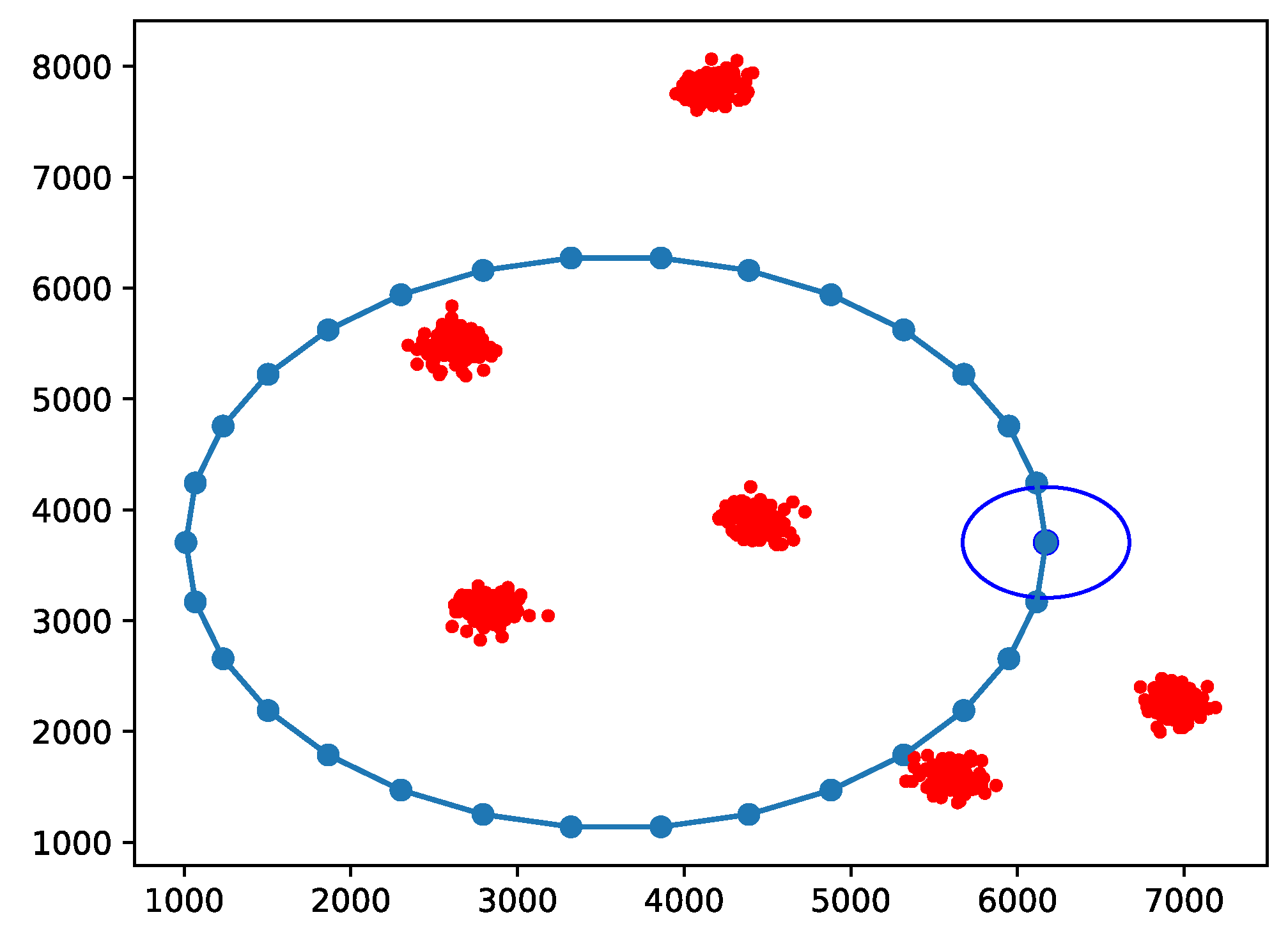
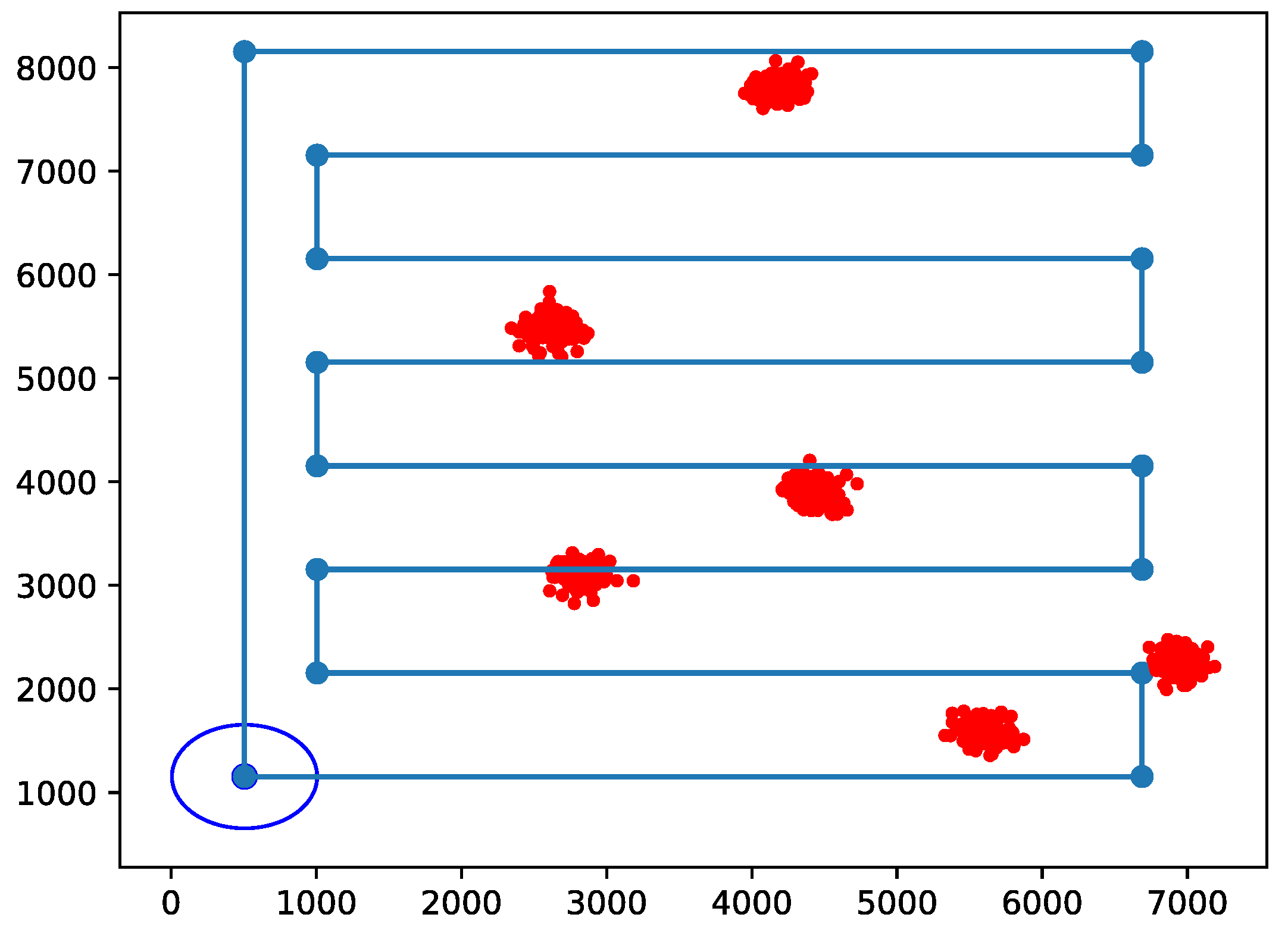
Figure 2.
Example of circular path (blue line) and clusters with nodes (red dots) location; the dark blue circle indicates the start of the trajectory.
Figure 2.
Example of circular path (blue line) and clusters with nodes (red dots) location; the dark blue circle indicates the start of the trajectory.
Figure 3.
Example of Paparazzi path (blue line) and clusters with nodes (red dots) location; the dark blue circle indicates the start of the trajectory.
Figure 3.
Example of Paparazzi path (blue line) and clusters with nodes (red dots) location; the dark blue circle indicates the start of the trajectory.
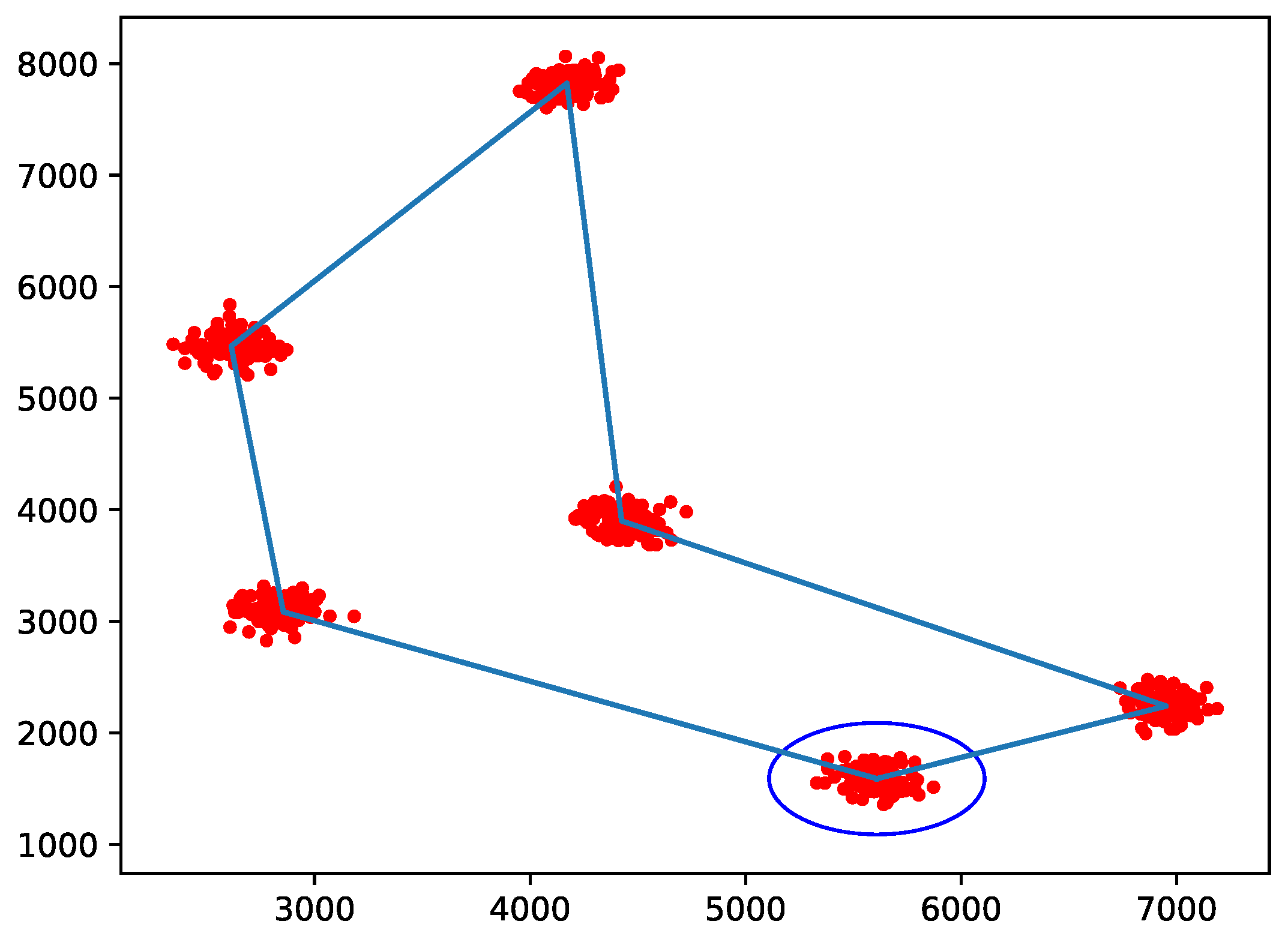
Figure 4.
Example of TSP-driven path (blue line) and clusters with nodes (red dots) location; the dark blue circle indicates the start of the trajectory.
Figure 4.
Example of TSP-driven path (blue line) and clusters with nodes (red dots) location; the dark blue circle indicates the start of the trajectory.
As one can easily see, the performance of the considered network depends both on the UAB mobility pattern and the UAB NB-IoT cell configuration. In the following section we consider how the respective parameters (e.g., UAB height and speed, NB-IoT coverage class configuration and cluster dimension) affect the performance.
5. Results and Discussion
In this section, we will analyze our NB-IoT network performance and discuss the achieved results. Simulations are carried out with the parameters listed in
Table 4. As previously mentioned, we are jointly studying a number of metrics, being:
the access rate, ;
the percentage of nodes completely served, ;
the mean latency perceived by nodes, ;
the network throughput, ;
the mean energy consumption of NB-IoT nodes, E.
These metrics are computed via the following formulas:
We denote as access rate,
in Equation (
8), the fraction of the number of succeeded transmissions,
, over the overall attempted by anyone of the IoT nodes,
. In this way, we analyze how frequently a node
u may get access to the channel. When the
value gets close to zero, the number of access attempts has to increase before success. Equation (
9) let us identify how effective is the UAB service. In fact,
counts the number of nodes successfully transmitting their traffic demand over the total number of present IoT nodes,
, in percentage. Then, Equation (
10) computes the latency or delay for the node
u spanning from the time in which the request is started,
, until when the transmission succeeded,
. If a node is not able to transmit its packet, we do not consider it in the average latency computation. Equation (
11) computes the overall network throughput by summing the one of each node
u,
. Finally, Equation (
12) averages the energy consumed by all nodes present in the service area,
.
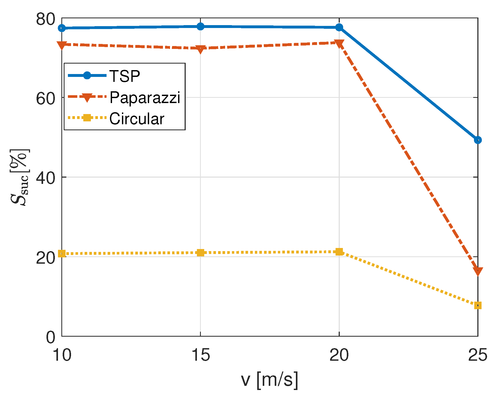
To start with,
Figure 5 shows the percentage of IoT nodes served by the UAB, that means their traffic demand is completely fulfilled. Its value is represented while varying the UAB speed,
v, and for the different trajectories. This picture has some relevant outcomes. First, the performance is not the same when varying speed; for each trajectory, it drops fairly below the 50% of served nodes. This is clearly related to the time interval in which the UAB is able to maintain a robust radio connection with each node. In fact, if the received power falls below the receiver sensitivity before the signalling is completed and the node is scheduled an uplink resource on the NPUSCH (for example, if the UAB has flown away too fast), it will not be able to successfully transmit its packet. This effect becomes relevant when discussing latency, because the value of
v creates a trade-off between low application delays and successful transmissions. At first glance, it is also evident that the TSP trajectory is able to serve a higher number of nodes for every UAB speed, making more robust what first proposed in [
1]. In fact, this trajectory ensures the UAB gets in close vicinity with each cluster and each node, while minimizing the distance travelled. On the opposite, the circular trajectory decreases the percentage of successful transmissions of 50% with respect to TSP and Paparazzi ones, on average. The coverage extension and the time spent over each node, does not allow in this case a sufficient service. The analysis on the other metrics would allow us to finally assess and discuss the final trajectory-dependent performance.
Figure 6 represents the access rate,
, again while varying the UAB speed for different trajectories. By looking at increasing speeds and for the same trajectory, we have the value of
dropping for each trajectory at 25 m/s, as it was for the service in
Figure 5. With the UAB driving faster, the occasions to attempt channel access decrease. From Equation (
8), we observe this metric evaluates together the number of overall attempts tried by nodes and, from these, the ones which are successful. This might explain why the Paparazzi and circular trajectories have higher access rates; these can be achieved if the total number of attempts is small (the denominator) with respect to other trajectories. If a lower number of nodes try to access at the same time to the channel (maybe for connectivity issues) the probability of successful transmission increases (see Equation (
1)).
Then, another figure of merit is the latency with which packets are transmitted (on average),
, in
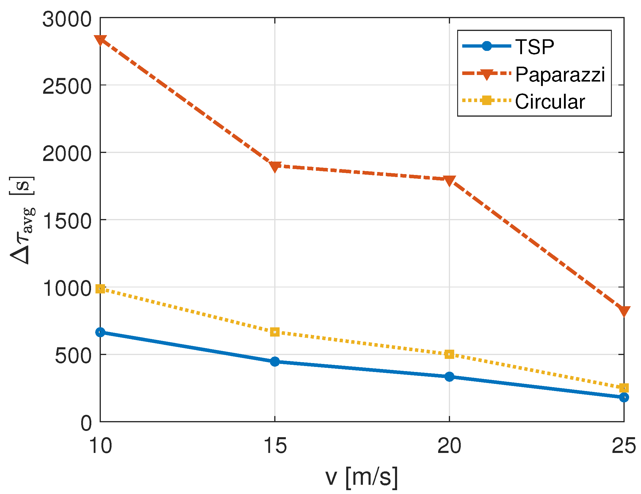
Figure 7. As expected, the latency decreases with increasing speed for each trajectory; the NB-IoT nodes which can successfully transmit their packet are served faster because the UAB will reach them with a smaller delay. Furthermore, if we focus on the latency of the different trajectories, we notice the TSP path performs better, just followed by the circular one. In fact, the distances covered by these two trajectories are fairly smaller with respect to the other. On the contrary, for its characteristic of scanning the entire service area, the Paparazzi trajectory employs much larger delays than the other two.
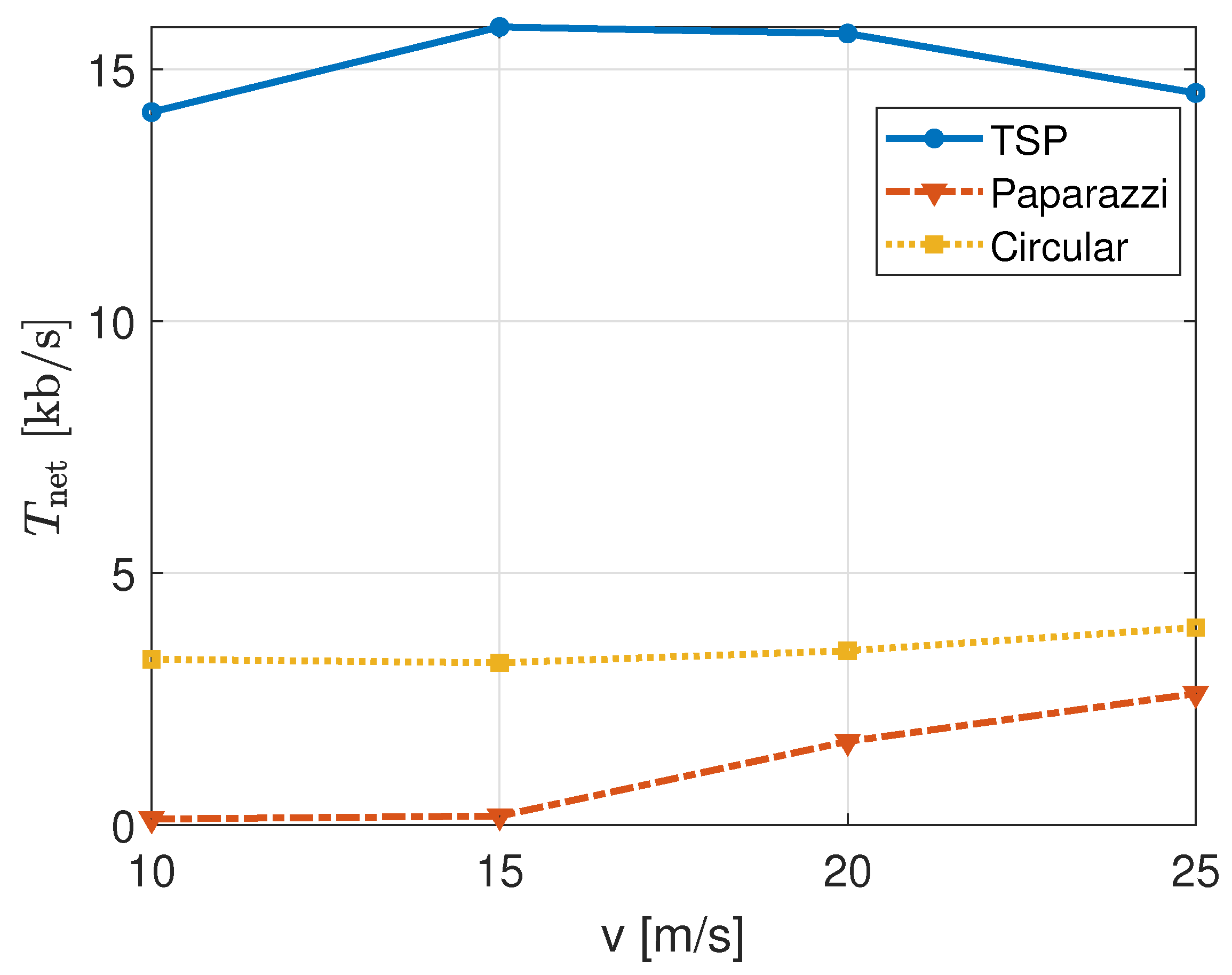
Furthermore, we are interested in the network throughput,
, that can be achieved. Numerical results are presented in
Figure 8. As formulated in Equation (
11), these results will also depend on the ones of
Figure 5 and
Figure 7 because of the dependence on service completion and latency in Equation (
6). Interestingly, we can see three different trends with varying UAB speeds,
v, for the three different trajectories: (i) The TSP has a maximum, (ii) the circular does not change significantly, while (iii) the Paparazzi shows an improvement with increasing velocities. The maximum shown by the network throughput in the TSP trajectory corresponds exactly to the service-latency trade-off with UAB speed mentioned before. However, because of the low total service offered, the circular trajectory is hardly showing any maxima. Similarly, the maximum cannot be appreciated for the Paparazzi path, but the network throughput appears to be increasing with increasing speed. In fact, we observed that, at lower UAB speeds as 10 to 15 m/s, the average latency is so large (almost one or a half hour) that the maximum cannot occur for the chosen UAB speed range. As expected, the TSP trajectory shows a relevantly higher throughput with respect to the other two, up to 16 kb/s. Moreover, because of a much larger average latency, the Paparazzi trajectory achieves an even lower throughput than the circular one (that had a much worse percentage of served nodes).
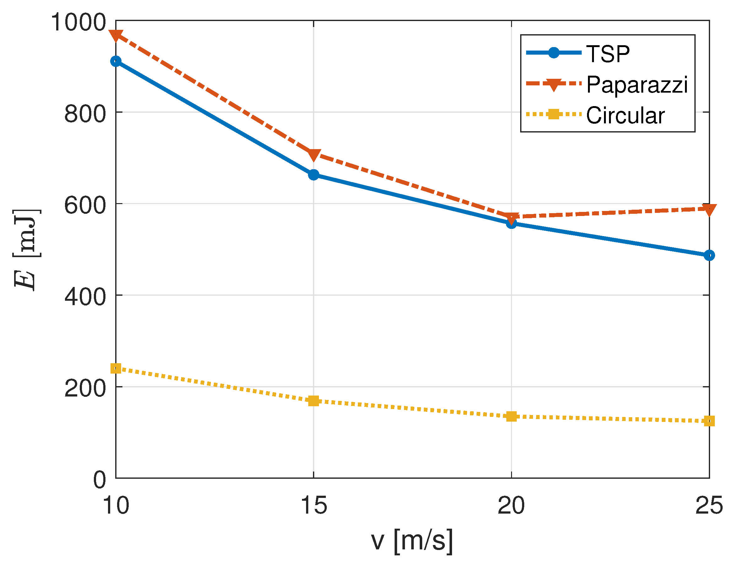
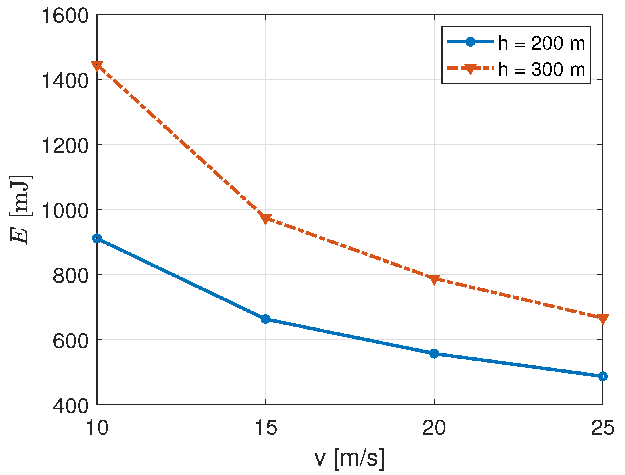
As last performance metric, we study the impact of trajectories on the average energy consumption,
E, in
Figure 9. For decreasing values of the UAB speed,
v, the energy consumed by NB-IoT nodes tend to decrease until few hundreds of mJ. Even if this appears to be a positive effect, we should consider the motivations behind this behaviour.
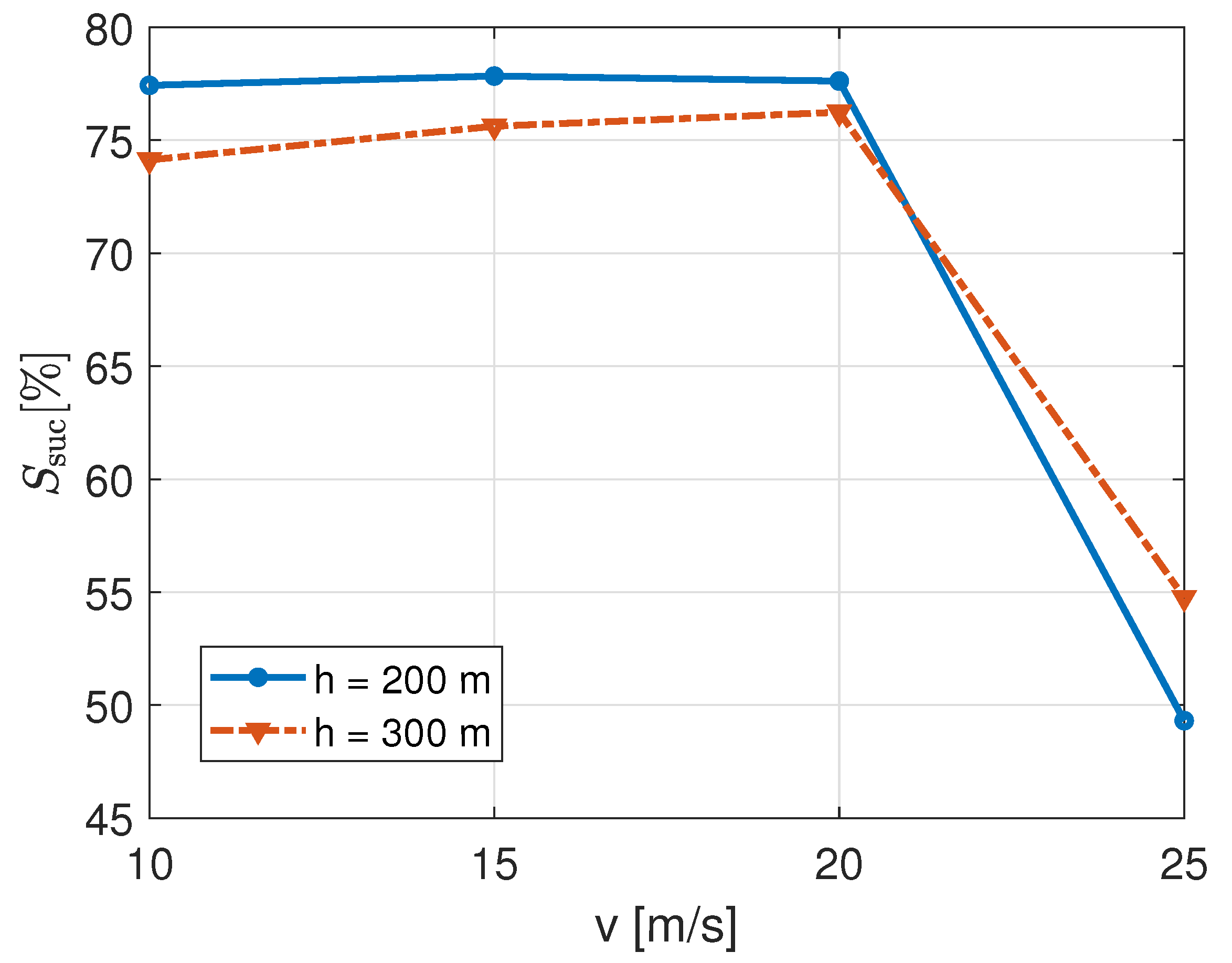
To avoid cluttering, we now show the impact of two different UAB heights, h, for the same trajectory. The TSP path is the trajectory chosen for its better results in terms of almost all metrics.
In this case, the percentage of served NB-IoT nodes with varying UAB speed,
v, is plotted in
Figure 10. The behaviour of the two curves with respect to speed is the same as already discussed in
Figure 5. However, we can see a slight difference from before, that is a lesser sharp decrease of successful transmissions when the speed is 25 m/s. We observe that for lower speeds the system performs better at lower UAB heights,
h, while for higher speeds increasing heights improve the service. One might expect that, since for higher altitudes the transmitter-receiver distance increases on average, the curve with the larger UAB height would perform always worse than the other (as it happens for values of
v lower than or equal to 20 m/s). However, this does not consider the NB-IoT signalling messages procedure and timing. In fact, for increasing values of
h, not only the transmitter-receiver distance gets higher, but also the coverage range of the UAB increases (given by the angle of incidence of the UAB with the ground, or elevation angle in [
7,
8]). Consequently, it increases the time interval during which, on average, the NB-IoT node remains in the coverage range of the UAB. As shown in
Figure 10, this effect can be more appreciated with increasing values of speed.
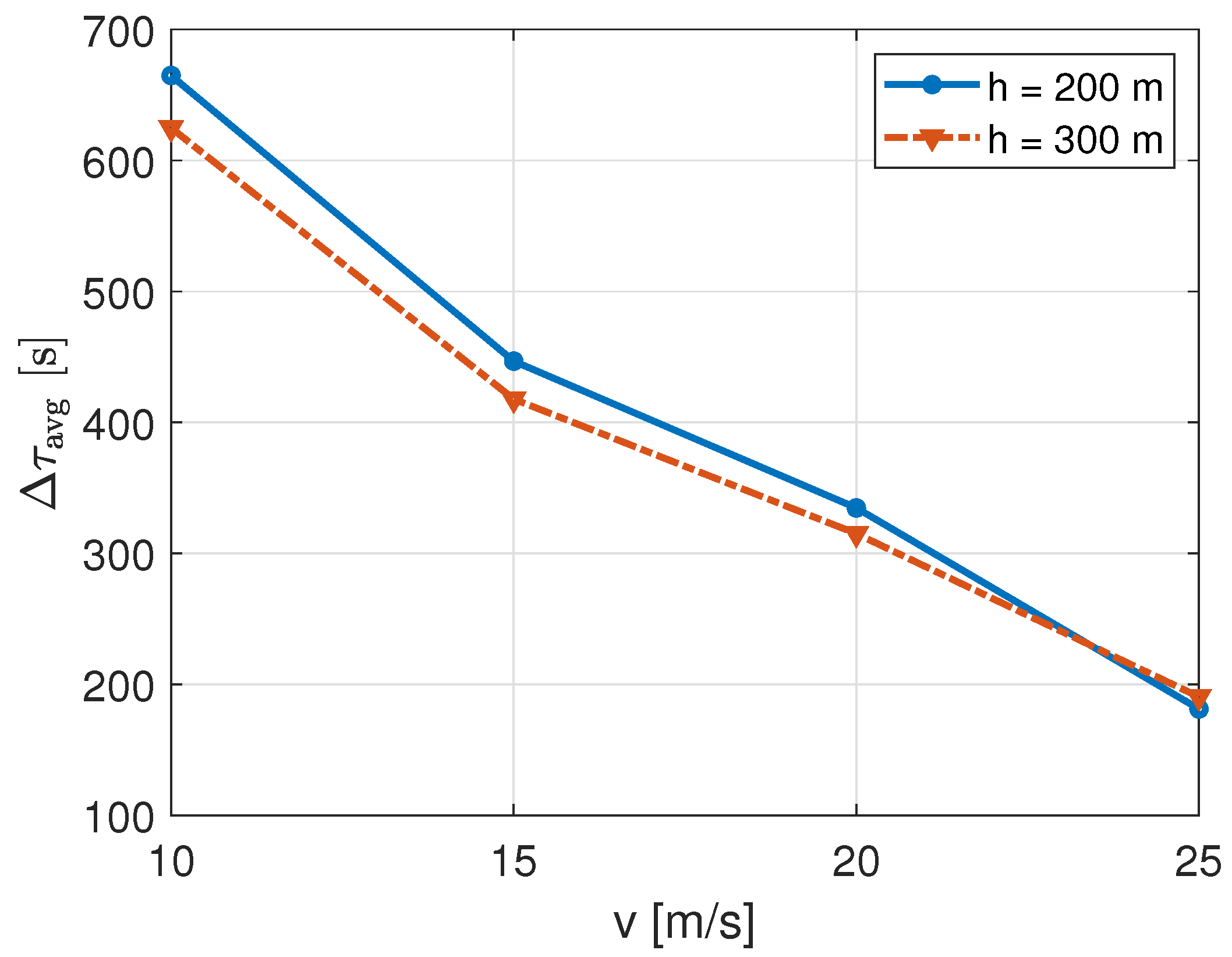
What has been discussed above is confirmed in
Figure 11, showing the average energy consumption,
E, with varying UAB speeds and heights. Being an average, its value depends on the number of nodes able to reach the UAB connectivity and enter the RA (i.e., signalling) procedure. The curves’ decreasing trend with speed is the same for the two
h values, and was already discussed for the TSP in
Figure 9. A higher altitude lets a larger number of nodes being in connectivity with the UAB, and try and start the RA procedure. This fact increases the overall energy consumption, regardless of successful transmission or not. With lower speeds, more nodes would be able to complete the signalling procedure, whether with higher speeds the energy consumed could be only for the transmission of NB-IoT Msg1 and/or Msg2.
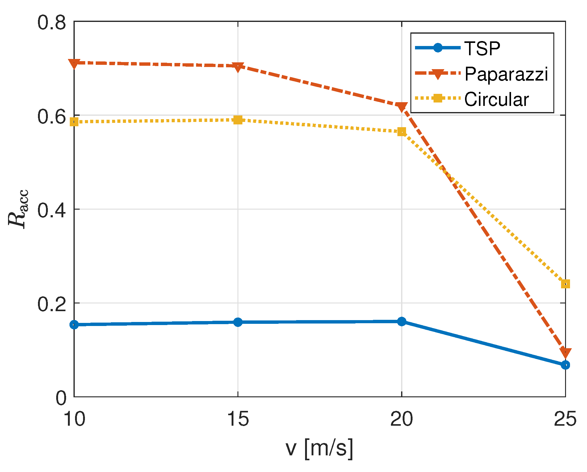
Our analysis on the energy consumption can be validated by
Figure 12. It represents the access rate,
, for different UAB heights and speeds in the TSP trajectory. Here, the curves trend with respect the to speed,
v, is the same, as for
Figure 11, and the curve with the higher height,
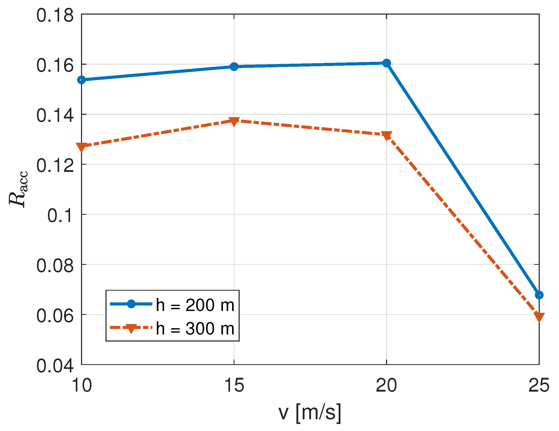
h, has a lower access rate. This means that we have a larger number of attempts that does not correspond to the same number of successful transmissions. In fact, also due to the average larger transmitter-receiver distances with a higher-height UAB, it gets more difficult for nodes to complete the RA procedure.
Related to average latency,
, we observe a quite less significant impact. In
Figure 13, the value of
is affected more by increasing UAB speeds rather than increasing UAB heights.
To summarize our findings into three main points, which reflect the previously mentioned key contributions, we can state that:
Simulations performed have accounted for all the described NB-IoT standard parameters, from the random access procedure to the precise scheduling in uplink transmission with the three NB-IoT coverage classes;
we jointly investigated a number of performance metrics related to the IoT field, namely (i) the number of completely served nodes, (ii) the achieved network throughput, (iii) the perceived latency and (iv) energy consumption of nodes. Numerical values achieved are related to the scenario under consideration and may scale accordingly. Different IoT applications may prefer one metric over the others as its main requirements, but our results show that pursuing one usually improves also the other metrics;
as evinced from the analyzed results, the TSP trajectory performs better than the others in terms of successful transmissions, latency and throughput, making it the most promising among the three for cellular IoT (e.g., NB-IoT) applications. As expected, the prevailing trajectory in terms of performance is scenario-dependent. Moreover, in our results, one can extract the behaviour of UAV networks with respect to speed and height; in particular, the UAV speed should be taken under control, since it might abruptly decrease the performance metric if kept too high.
Thanks to our number of outcomes and simulations (and the variety of real scenarios that could apply to our system model), we can discuss results further and broaden our findings to different cases.
In the numerical evaluation, we first identify which are the relevant factors an operator must take into account when deploying this kind of system. First, the speed undergoes a trade-off between average perceived latency and throughput from one side to total number of successfully served nodes on the other. In this sense, the NB-IoT protocol plays a relevant role, since too higher speeds do not allow the completion of the RA procedure, and therefore the scheduling of uplink resources in the NPUSCH. Moreover, though a larger altitude would grant an increased NB-IoT nodes connectivity, increases the transmitter-receiver distance, which has again a negative impact on the successful completion of the RA procedure.
From our results, we can also infer conclusions on the trajectory selection. We can state that the circular trajectory, as would be for any path that travels the perimeter of a convex figure, is neither an effective trajectory in terms of latency nor a robust choice for the service of a massive number of IoT nodes. In fact, it is not able to follow the particular deployment of nodes for a given service area. On the other hand, a Paparazzi trajectory seems a good alternative, since it ensures to scan the overall service area. This might be a fair solution if a mobile operator does not know a priori the location of nodes. However, because of the fact that this information is usually easy to retrieve and that the Paparazzi trajectory becomes expensive in terms of energy consumption and latency, is probably not desirable. This confirms the expectations on the robustness of the TSP path.
If we want to achieve the 100% successfully served nodes, the use of multiple UABs might be necessary. However, this can apply only for those trajectories reaching full nodes connectivity, as for the case of TSP and Paparazzi. In fact, an n-th UAB, following the path of its predecessors, will address only those nodes not previously served. This fact would lighten the access procedure, since there will be less nodes contending and more radio resources available in a smaller time interval. In fact, a similar behaviour with respect to speed in
Figure 5 and
Figure 6 suggests that the number of access attempts may be a tighter bottleneck than the time needed for signalling. Multiple UABs may lower the traffic load allowing a larger number of nodes to get access to the channel.


