Abstract
The development of UAV technologies offers practical methods to create landcover maps for monitoring and management of areas affected by natural disasters such as landslides. The present study aims at comparing the capability of two different types of UAV to deliver precise information, in order to characterize vegetation at landslide areas over a period of months. For the comparison, an RGB UAV and a Multispectral UAV were used to identify three different classes: vegetation, bare soil, and dead matter, from April to July 2021. The results showed high overall accuracy values (>95%) for the Multispectral UAV, as compared to the RGB UAV, which had lower overall accuracies. Although having lower overall accuracies, the vegetation class of the RGB UAV presented high producer’s and user’s accuracy over time, comparable to the Multispectral UAV results. Image quality played an important role in this study, where higher accuracy values were found on cloudy days. Both RGB and Multispectral UAVs presented similar patterns of vegetation, bare soil, and dead matter classes, where the increase in vegetation class was consistent with the decrease in bare soil and dead matter class. The present study suggests that the Multispectral UAV is more suitable in characterizing vegetation, bare soil, and dead matter classes on landslide areas while the RGB UAV can deliver reliable information for vegetation monitoring.
1. Introduction
The evolution of remote sensing technology allows a feasible method for gathering detailed information for mapping land-cover changes [1], drought monitoring [2], and analyzing complex attributes [3,4] over space and time. This technology uses different types of sensor onboard satellites, airborne or unmanned aerial vehicles (UAVs), and provides different methods of vegetation classification at large and small scales. Remote sensing offers a practical approach to designing strategies for the management of forest disaster such as evaluating landslide-prone areas through airborne, UAV, and ground-based remote sensing [5], as well as for evaluating changes in vegetation cover after a wildfire for post-fire management by using satellite-based remote sensing and UAV [6].
To deal with the need to assess forest disasters for quick management decisions, the advancement of satellite-based remote sensing applications was initiated for detecting areas affected by natural disasters such as windthrow and landslide for forest restoration or forest disaster management purposes [7], assessing vegetation recovery [8], detecting and mapping [9,10] of landslide areas, and creating historical landslide inventories [11]. Although playing an important role in forest disaster management, satellite-based remote sensing has some limitations in terms of spatial and temporal resolution of the data. Local cloudiness, low temporal and spatial resolution, and gaps on the image create a complex task for vegetation classification [2,12,13]. Recently, very high spatial resolution satellites are available, delivering data of around 30 cm per pixel [14]; despite a high spatial resolution, this could be a limitation in understanding changes happening on smaller scales [15]. A one-day temporal resolution satellite dataset is also available [16], but cloud cover can still be a hindrance to acquiring the desired dataset.
Nevertheless, the evolution of UAV technologies has brought RGB sensors and multispectral sensors to UAVs for more detailed information as compared to satellite-based remote sensing, making it possible to acquire centimeter-level imagery at any time. In terms of cost and availability, multispectral UAVs cost much more and have lower availability while UAVs coupled with RGB sensors are more affordable and accessible. However, RGB UAVs are limited for remote sensing analysis, especially on complex and heterogeneous forest-covered areas, due to the sensor having an RGB array filter [17]. Despite these limitations, Ruwaimana et al., [18] proved that the application of UAVs for vegetation classification on mangrove ecosystems provided higher accuracy concerning object-based and pixel-based classification compared to satellite imagery. The implementation of UAV systems gained attention not only due to their efficiency to map land cover [19,20] vegetation on a coastal dune [21] but also as an effective tool in mapping and characterizing burned areas affected by wildfires [22], as well as landslide displacement mapping [23].
Comparing the performance between satellite image and aerial photo for vegetation mapping [18], testing the applicability of UAVs for mapping and monitoring geohazard areas [24], as well as characterizing and monitoring landslides, [25] have been well documented. Yet there is still a gap in understanding how RGB and multispectral sensors on UAVs perform in assessing the regrowth of vegetation in an area affected by a natural disaster such as a landslide. In order to understand the condition of the affected area to make management decisions, it is important to determine the vegetation coverage to understand its regrowth on a landslide area on a small scale [26,27], and to evaluate the area’s ability to undergo a natural regeneration process on a regional scale. Besides, the presence of debris including fallen logs and litter provides a potential for vegetation regrowth by sprouting and seedbanks [28] and by the colonization of early successional plant species [29,30,31]. Moreover, due to unstable bare soil conditions, vegetation regrowth is slow or non-existent on hillslopes [32].
Therefore, we mapped a landslide area considering three different classes (i.e., vegetation, bare soil, and dead matter) to assess the changes in coverage pattern focusing on vegetation growth throughout four months using two different types of UAV. This study aimed to compare the performance of an RGB UAV and a multispectral UAV using a pixel-based classification approach, to understand how the spectral resolution and the type of sensor can deliver precise information for vegetation mapping on a landslide area. The findings from this study can provide baseline information for forest managers and ecologists in selecting the applicable system and to assist in deciding on further management practice in the affected area, especially in understanding post-landslide regeneration. Thus, this study was designed for the following objectives: (1) to understand the differences between the UAV systems for vegetation mapping in a landslide area assessing the parameters that affect the datasets; (2) to monitor the monthly changes of vegetation, bare soil, and dead matter areas in landslides for the management of vegetation recovery.
2. Materials and Methods
2.1. Study Area
In 2018, the northernmost island of Japan, Hokkaido, was affected by the Hokkaido Eastern Iburi Earthquake, with a magnitude of 6.7 [33] and several aftershocks. The seism triggered over 4000 ha of landslides around different municipalities in western Atsuma town [34].
This study was conducted in an area of surface failure of approximately 8 ha in the Uryu District at Atsuma town (42°43′20.3″ N, 141°55′22.5″ E) (Figure 1). The area was characterized by moderate terrain with a predominant slope and an angle of less than 40 degrees, and the elevation ranged from 57m to 121m. Soil structure consists of Neogene sedimentary rock, i.e., sandstone, siltstone, mudstone, and a conglomerate that was covered by a thick pyroclastic fall deposit from the Tarumae Volcano [34,35]. The area was covered mostly by deciduous trees, fallen trees, and bare soil, an effect of the landslide, with grasses and shrubs such as Japanese sweet-coltsfoot (Petasites japonicus (Siebold et Zucc.) Maxim.), dwarf bamboo (Sasa spp.), and wild berries (Rubus spp.), etc.
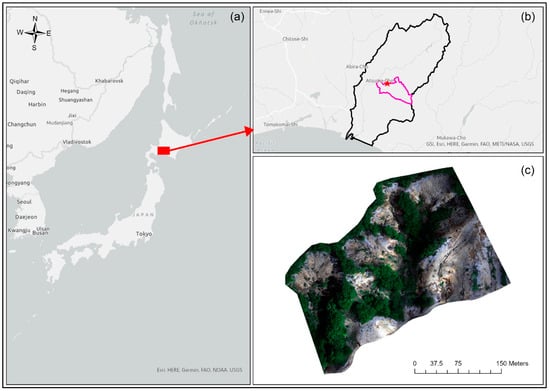
Figure 1.
(a) The study area located in Hokkaido, Japan, (b) at Atsuma town (black boundary), and in Uryu district (pink boundary) located at 42°43′20.3″ N, 141°55′22.5″ E (red star); (c) with the true color ortho-mosaic taken with the Multispectral UAV on 9 June.
2.2. Datasets
For acquisition of the aerial images to create the ortho-mosaics for analysis, two different UAVs were used: the DJI Phantom 4 Pro, and the DJI Phantom 4 Multispectral. The DJI Phantom 4 Pro has a 1-inch CMOS RGB sensor, which acquires the red, green, and blue wavelengths in the same sensor, delivering one 5472 × 3648 pixels RGB image per shot. On the other hand, the DJI Phantom 4 Multispectral, has six 1/2.9-inch CMOS sensors, one RGB sensor for visible imaging and five monochrome sensors for multispectral imaging in different spectral bands: blue, green, red, red-edge, and near-infrared. Each band generates one image of 1600 × 1300 pixels, totalizing six images per shot. The DJI Phantom 4 Multispectral also had a Real-Time Kinect (RTK) GNSS system built in for centimeter position accuracy, but for this study, we compared only the sensors of each UAV: the RGB sensor of DJI Phantom 4 Pro (RGB UAV) and the multispectral sensor from DJI Phantom 4 Multispectral (Multispectral UAV).
The data was taken in four different flight campaigns in 2021: 14 April, 12 May, 9 June, and 9 July, with all images taken in the morning. The weather condition on 14 April and 9 July was cloudy, while being sunny on 12 May and 9 June, with no clouds (Figure 2).
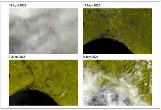
Figure 2.
Cloud cover over the study site (red star) in each date, assessed using Modis M0D09GQ.006 Terra Surface Reflectance Daily Global 250 m, acquired in the morning [36].
For each flight campaign, we first flew the Multispectral UAV followed by the RGB UAV (around 14 min each flight), with 5 min in between flights to reduce the displacement of shadow areas. The UAVs were flown at 120 m of altitude, capturing images with 80% overlap and 80% side-lap to create the ortho-mosaics via photogrammetry processing. For the Multispectral UAV, images of a calibration reflectance panel were taken to be used on the calibration of the multispectral images inside the photogrammetry software [37].
To register the RGB and Multispectral ortho-mosaics, 15 ground control points (GCPs) made from plywood were placed along the study site and the position of each point was collected using the Drogger RTK GNSS system [38] connected to the ICHIMILL virtual reference station (VRS) [39] service provided by Softbank Japan [40]. The accuracy of each point position was around 2 cm.
For each flight campaign, a field survey was also conducted. Using the Drogger RTK system connected to an android tablet with the open-source application Open Data Kit (ODK) [41], we collected ground truth points to classify the ortho-mosaics and validate the classification results. Inside the ODK application, a questionnaire form was previously created containing the classes to be chosen on the field, and photos were taken with the tablet (Figure 3).
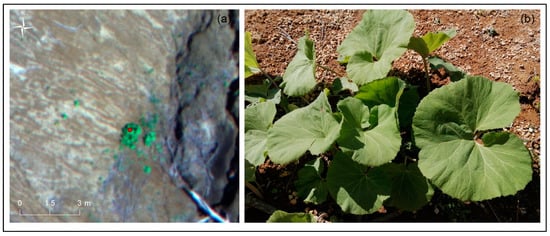
Figure 3.
(a) The red dot is the vegetation class obtained by ODK with the RTK system accuracy (2 cm) on the Multispectral UAV ortho-mosaic in true color, and (b) the respective photo of a Japanese sweet-coltsfoot for verification on 12 May.
2.3. Data Processing
To create the ortho-mosaics, we used the photogrammetry technique for UAVs [42], where each image dataset was processed on Agisoft Metashape [43] with the GCPs taken on the field to improve the position accuracy of the ortho-mosaic. For the Multispectral UAV, the 5 monochrome images were automatically merged creating a multispectral ortho-mosaic, and the images were also calibrated in the software using the calibration reflectance panel images to convert the digital numbers into reflectance values. All ortho-mosaics were later uploaded into Google Earth Engine [44] and resampled to the same spatial resolution of 5.5 cm using the bilinear interpolation mode.
2.4. Classification and Accuracy Assessment
The processing workflow is shown in Figure 4. To identify vegetation cover in the study area, three different classes were established: vegetation, bare soil, and dead matter (dead leaves, fallen trees, and tree branches). To create the reference dataset, an empirical test was made and 30 samples for each class were selected to conduct the study. The reference dataset was composed of samples taken on the field and samples selected from a visual interpretation of the ortho-mosaic, totalizing 90 samples. For each date, the same reference dataset was used for the RGB and the multispectral dataset.
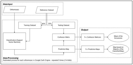
Figure 4.
The processing workflow for each dataset.
The classification and the assessment for this study were made by applying the cross-validation method [45], using 5 k-folds inside Google Earth Engine. The built-in support vector machine classifier with the linear kernel type [46] was selected to classify the ortho-mosaics. This method was chosen due to its robustness in assessing the predictor model, which in this study was mainly influenced by the ortho-mosaic.
First, the reference data was divided into five different folds randomly, where four folds (80% of the reference dataset) were used to train the classifier and one fold (20% of the reference dataset) to test the classifier. A total of five iterations were made to test all folds.
For each iteration, we created a classification model based on the training dataset and the support vector machine classifier. Then, the classification model generated a prediction map which was put against the independent testing dataset to achieve a confusion matrix. The confusion matrix delivered three different results: overall accuracy, producer’s accuracy (PA), and user’s accuracy (UA).
The final assessment values for each ortho-mosaic were created considering the mean of the accuracies of all five confusion matrices. To create the final classification map of each ortho-mosaic, an aggregation was made considering the majority of classes among the five iterations for each pixel; the final classification map presented a straightforward portrayal of confidence for the study site, which identified the model’s fit and stability. Whilst not directly measuring mapping accuracy, the relative confidence of the methodology can provide valuable information to support the interpretation of the maps [47].
3. Results
3.1. UAV Orthomosaics
Figure 5 shows that the higher spatial resolution of the RGB UAV created ortho-mosaics with more details compared to the Multispectral UAV ortho-mosaic, even though the data were resampled to 5.5 cm.
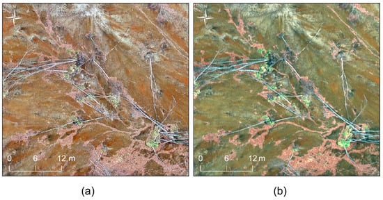
Figure 5.
(a) The RGB UAV in true color ortho-mosaic resampled to 5.5 cm, (b) the Multispectral UAV in true color ortho-mosaic resampled to 5.5 cm. The RGB UAV ortho-mosaic has a sharper image compared to the Multispectral UAV ortho-mosaic.
The RGB and Multispectral UAV ortho-mosaic colors and amount of shadow were also influenced by the weather condition (Figure 2). Due to the cloudy condition and rain on the previous days of 14 April and 9 July [48,49], the ortho-mosaics were generated with brownish soil and without any shadow effect. During the sunny condition on 12 May and 9 June, the ortho-mosaics were generated with whitish soil and shadow effects (Figure 6).
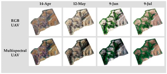
Figure 6.
The RGB UAV and Multispectral UAV ortho-mosaics generated by Agisoft Metashape on 14 April, 12 May, 9 June and 9 July. The soil color on 14 April and 9 July was brownish with no shadow, while on 12 May and 9 June, the soil was whitish with shadow areas.
3.2. Performance of the UAV’s Imagery
The performance of the UAV’s imagery was accessed considering the overall accuracies calculated from the mean of all five K-folds of each dataset (Table 1). The Multispectral UAV delivered higher percentages (more than 95%) throughout the months. On the other hand, the RGB UAV presented slightly lower overall values, with the highest values on 14 April (94.44%) and on 9 July (90%), while for pm 12 May and 9 June, the values were 72.22% and 64.44% respectively.

Table 1.
Overall accuracies for the Multispectral UAV and RGB UAV on each date with the respective weather condition.
Looking into the PA and UA of all classes (i.e., vegetation, bare soil, and dead matter) (Table 2), the RGB UAV had the highest values for the three classes on April 14th and July 9th, while lower values were found on 12 May and 9 June, mainly on bare soil and dead matter classes. The Multispectral UAV was more consistent compared to the overall accuracies in Table 1, and both PA and UA showed high values throughout the months for all three classes, above 90%.
Table 2.
Producer’s and user’s accuracy of the vegetation, bare soil, and dead matter classes.
3.3. Classification Results
The classification results created through the aggregation considering the majority classes for the five prediction maps are shown in Figure 7.
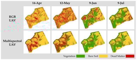
Figure 7.
Classification results from the Multispectral UAV and the RGB UAV on each date.
Despite the high accuracy values on the Multispectral UAV, the visual interpretation showed some disparities when compared to the respective ortho-mosaics (Figure 8). Misclassification mainly occurred on the shadowed area (Figure 8a), where both bare soil and dead matter areas were misclassified as vegetation class (Figure 8b).
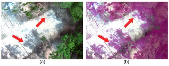
Figure 8.
(a) The Multispectral UAV ortho-mosaic in true color on 9 June, (b) vegetation class (pink), misclassifying bare soil and dead matter areas (red arrows).
The RGB UAV generated more misclassification throughout the study area. On 12 May and 9 June, it was clear to see the misclassification of the dead matter class on bare areas (Figure 6 and Figure 7). A closer look on 12 May (Figure 9) showed misclassification occurring even in no shadow areas.
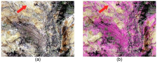
Figure 9.
(a) The RGB UAV ortho-mosaic in true color on 12 May, (b) the dead matter class (pink), misclassifying bare areas (red arrows).
The comparison among the classified maps in terms of class coverage (i.e., vegetation, bare soil, and dead matter) over the months, showed a similar pattern in the RGB UAV and the Multispectral UAV from April to June (Figure 10), where we found an increase in the vegetation class and a decrease in both bare soil and dead matter classes.
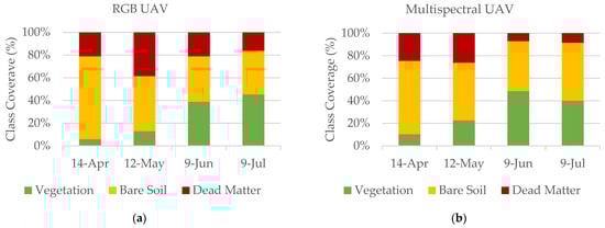
Figure 10.
The graph shows the class coverage (%) generated from the (a) RGB UAV and (b) Multispectral UAV over time.
In the Multispectral UAV, the proportion for the vegetation class on 9 June was higher when compared to 9 July, while values for bare soil increased during the same period. This was due to the misclassification that happened in the shadowed area of 9 June (Figure 8). Another problem also occurred on the RGB UAV, where there was an increase in the dead matter class from 14 April to 12 May, misclassified by the inclusion of the dead matter class on bare areas (Figure 9).
Comparing the vegetation class of RGB UAV and Multispectral UAV, besides presenting high values of PA and UA, it was possible to see a similar pattern of vegetation growth around the already vegetated areas (Figure 11). On the other hand, for the bare soil and dead matter classes, the similarities were much smaller when comparing the RGB UAV and the Multispectral UAV (Figure 12 and Figure 13), as expected by the low values of the PA and UA accuracies from these classes on the RGB UAV.
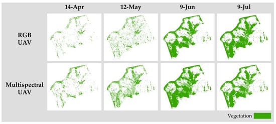
Figure 11.
Change of vegetation class over the months from the RGB and multispectral UAV.
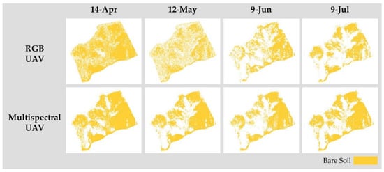
Figure 12.
Change of bare soil class over the months from the RGB and multispectral UAV.
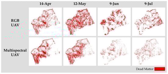
Figure 13.
Change of dead matter class over the months from the RGB and multispectral UAV.
4. Discussion
4.1. Comparison between the RGB UAV and the Multispectral UAV
The evaluation of the performance of each UAV showed that the Multispectral UAV delivered more consistent results for every class, while the RGB UAV, even though more detailed (higher spatial resolution), suffered from the smaller number of bands and the type of sensor [50], generating a more speckled classification map. On the other hand, even though having five distinct spectral bands and higher accuracy values, the Multispectral UAV generated some misclassification, mainly on shadowed areas [51,52].
Apart from the misclassification of shadowed areas, the weather conditions played an important role in this study, mainly for the RGB UAV. Cloudy days with brownish soil had better results compared to sunny weather with whitish soil, delivering higher accuracy values for both RGB UAV and Multispectral UAV. This was also confirmed by Duffy et al. [51], which suggests that cloudy days had consistent lighting conditions, improving the homogeneity of the spectral signatures.
Even though the RGB UAV and the Multispectral UAV generated misclassifications, they could still provide valuable information regarding the monitoring of classes’ coverage changes on a landslide area. The RGB UAV delivered impressive results, being able to monitor vegetation growth in detail despite the low cost of the system. Although the visual analysis showed a discrepancy between the RGB UAV classification map and the respective ortho-mosaics on the bare soil and dead matter classes, when comparing the area of coverage by the classes both UAV systems had similar patterns, with the vegetation class reflecting a gradual increase from April to June along with the decrease in bare soil and dead matter classes over these months.
Considering the pixel-based classification approach, the Multispectral UAV is recommended, due to its ability to acquire data on the red edge and near-infrared wavelengths, optimal for vegetation analysis. On the other hand, the higher spatial resolution of the RGB UAV could enable a more accurate visual inspection of the geohazard areas as reported by Rossi et al. [24]. Future studies using an object-based classification approach are suggested to understand the difference between the two UAV systems considering spatial resolution [18]. Therefore, both the RGB UAV and the Multispectral UAV proved suitable for evaluating the capability of the area to undergo a natural regeneration process, at a centimeter-level.
4.2. Vegetation, Bare Soil, and Dead Matter Monitoring
The results showed not only the possibility of monitoring changes throughout the months, but also locating where the changes happened. This is key since monitoring pattern changes from dead matter to vegetation class could provide an initial understanding of the potential of vegetation regeneration on the landslides area. The applied methodology also proved suitable for areas with a dominance of deciduous forest, where the identification of the dead matter was possible after the winter season when the trees had no foliage.
The vegetation growth around the already vegetated areas confirms that the condition of unstable soil after landslides, preventing seeds from nearby intact forests to germinate due to the erosion of soil, infertile soil, and other abiotic factors, slows down or impedes the regeneration process. The availability of decomposing material, i.e., fallen trees and leaf litter, favor the initial stage of plant succession on the landslide area [53,54] by protecting the seeds or saplings from rolling down due to soil erosion. as well improving soil fertility through the decomposition process.
The expansion in vegetation coverage observed during the four consecutive months could indicate that a post-landslide regeneration occurred in the affected area. This suggests that the increase in vegetation recovery on the landslides area might improve stability, especially on the bare soil area, in order to support seed germination and the growth of saplings, though this process would take a long time [53,55]. Thus, monitoring the pattern changes through time comparing the three classes, i.e., vegetation, bare soil, dead matter, contributes to a more detailed ecological research planning. Due to the role of landslide areas in regenerating high vegetation species richness after disturbance [55,56], the annual vegetation growth dataset is suggested to infer the potential of the study area for dynamic regeneration.
5. Conclusions
Overall, the present study reveals that Multispectral UAVs are more applicable for characterizing vegetation, bare soil, and dead matter in areas affected by landslides, highlighting that cloudy weather and brownish soil are recommended to create a more reliable dataset. However, the RGB UAV can play an important role if the purpose is to monitor vegetation development, which is a positive achievement, especially in terms of accessibility and availability of the tool. In addition, the monitoring of vegetation, bare soil, and dead matter classes over four months suggests the initial recovery of vegetation on the landslide area. This indicates that the monthly annual dataset and multi-year dataset will serve a better understanding of the dynamic process of initial vegetation recovery. Future work is suggested using an object-based classification approach, in order to take advantage of the higher spatial resolution of the RGB UAV dataset.
Author Contributions
Conceptualization, F.F., L.A.L. and J.M.; data curation, H.A.; formal analysis, F.F.; investigation, F.F. and H.A.; methodology, F.F.; project administration, F.F.; resources, M.K.; software, F.F.; supervision, M.K. and J.M.; validation, N.Y.; visualization, L.A.L.; writing—original draft, F.F. and L.A.L.; writing—review & editing, F.F., L.A.L., N.Y. and J.M. All authors have read and agreed to the published version of the manuscript.
Funding
This research received JSPS KAKENHI Grant Number JP17H01516 and TOUGOU Grant Number JPMXD0717935498.
Institutional Review Board Statement
Not applicable.
Informed Consent Statement
Not applicable.
Data Availability Statement
Not applicable.
Conflicts of Interest
The authors declare no conflict of interest.
References
- Hansen, M.C.; Loveland, T.R. A review of large area monitoring of land cover change using Landsat data. Remote Sens. Environ. 2012, 122, 66–74. [Google Scholar] [CrossRef]
- West, H.; Quinn, N.; Horswell, M. Remote sensing for drought monitoring & impact assessment: Progress, past challenges and future opportunities. Remote Sens. Environ. 2019, 232, 111291. [Google Scholar] [CrossRef]
- Blaschke, T. Object based image analysis for remote sensing. ISPRS J. Photogramm. Remote Sens. 2010, 65, 2–16. [Google Scholar] [CrossRef] [Green Version]
- Langner, A.; Titin, J.; Kitayama, K. The Application of Satellite Remote Sensing for Classifying Forest Degradation and Deriving Above-Ground Biomass Estimates. Angew. Chem. Int. Ed. 2012, 6, 23–40. [Google Scholar]
- Casagli, N.; Frodella, W.; Morelli, S.; Tofani, V.; Ciampalini, A.; Intrieri, E.; Raspini, F.; Rossi, G.; Tanteri, L.; Lu, P. Spaceborne, UAV and ground-based remote sensing techniques for landslide mapping, monitoring and early warning. Geoenviron. Dis. 2017, 4, 1–23. [Google Scholar] [CrossRef]
- Martinez, J.L.; Lucas-Borja, M.E.; Plaza-Alvarez, P.A.; Denisi, P.; Moreno, M.A.; Hernández, D.; González-Romero, J.; Zema, D.A. Comparison of Satellite and Drone-Based Images at Two Spatial Scales to Evaluate Vegetation Regeneration after Post-Fire Treatments in a Mediterranean Forest. Appl. Sci. 2021, 11, 5423. [Google Scholar] [CrossRef]
- Furukawa, F.; Morimoto, J.; Yoshimura, N.; Kaneko, M. Comparison of Conventional Change Detection Methodologies Using High-Resolution Imagery to Find Forest Damage Caused by Typhoons. Remote Sens. 2020, 12, 3242. [Google Scholar] [CrossRef]
- Lin, C.-Y.; Lo, H.-M.; Chou, W.-C.; Lin, W.-T. Vegetation recovery assessment at the Jou-Jou Mountain landslide area caused by the 921 Earthquake in Central Taiwan. Ecol. Modell. 2004, 176, 75–81. [Google Scholar] [CrossRef]
- Hervás, J.; Barredo, J.I.; Rosin, P.L.; Pasuto, A.; Mantovani, F.; Silvano, S. Monitoring landslides from optical remotely sensed imagery: The case history of Tessina landslide, Italy. Geomorphology 2003, 54, 63–75. [Google Scholar] [CrossRef]
- Chen, W.; Li, X.; Wang, Y.; Chen, G.; Liu, S. Forested landslide detection using LiDAR data and the random forest algorithm: A case study of the Three Gorges, China. Remote Sens. Environ. 2014, 152, 291–301. [Google Scholar] [CrossRef]
- Martha, T.R.; Kerle, N.; van Westen, C.J.; Jetten, V.; Vinod Kumar, K. Object-oriented analysis of multi-temporal panchromatic images for creation of historical landslide inventories. ISPRS J. Photogramm. Remote Sens. 2012, 67, 105–119. [Google Scholar] [CrossRef]
- Fuentes-Peailillo, F.; Ortega-Farias, S.; Rivera, M.; Bardeen, M.; Moreno, M. Comparison of vegetation indices acquired from RGB and Multispectral sensors placed on UAV. In Proceedings of the 2018 IEEE International Conference on Automation/XXIII Congress of the Chilean Association of Automatic Control (ICA-ACCA), Concepcion, Chile, 17–19 October 2018; pp. 1–6. [Google Scholar]
- Al-Wassai, F.A.; Kalyankar, N.V. Major Limitations of Satellite images. J. Glob. Res. Comput. Sci. 2013, 4, 51–59. [Google Scholar]
- MAXAR–CONSTELLATION. Available online: https://www.maxar.com/constellation (accessed on 30 July 2021).
- Woodcock, C.E.; Strahler, A.H. The factor of scale in remote sensing. Remote Sens. Environ. 1987, 21, 311–332. [Google Scholar] [CrossRef]
- Planet Labs Inc Satellite Imagery and Archive. Available online: https://www.planet.com/products/planet-imagery/ (accessed on 2 July 2021).
- Vanamburg, L.K.; Trlica, M.J.; Hoffer, R.M.; Weltz, M.A. Ground based digital imagery for grassland biomass estimation. Int. J. Remote Sens. 2006, 27, 939–950. [Google Scholar] [CrossRef]
- Ruwaimana, M.; Satyanarayana, B.; Otero, V.; Muslim, A.M.; Syafiq, A.M.; Ibrahim, S.; Raymaekers, D.; Koedam, N.; Dahdouh-Guebas, F. The advantages of using drones over space-borne imagery in the mapping of mangrove forests. PLoS ONE 2018, 13, e0200288. [Google Scholar] [CrossRef] [PubMed] [Green Version]
- Kalantar, B.; Mansor, S.B.; Sameen, M.I.; Pradhan, B.; Shafri, H.Z.M. Drone-based land-cover mapping using a fuzzy unordered rule induction algorithm integrated into object-based image analysis. Int. J. Remote Sens. 2017, 38, 2535–2556. [Google Scholar] [CrossRef]
- Bellia, A.F.; Lanfranco, S. A Preliminary Assessment of the Efficiency of Using Drones in Land Cover Mapping. Xjenza 2019, 7, 18–27. [Google Scholar] [CrossRef]
- Suo, C.; McGovern, E.; Gilmer, A. Coastal Dune Vegetation Mapping Using a Multispectral Sensor Mounted on an UAS. Remote Sens. 2019, 11, 1814. [Google Scholar] [CrossRef] [Green Version]
- Lazzeri, G.; Frodella, W.; Rossi, G.; Moretti, S. Multitemporal Mapping of Post-Fire Land Cover Using Multiplatform PRISMA Hyperspectral and Sentinel-UAV Multispectral Data: Insights from Case Studies in Portugal and Italy. Sensors 2021, 21, 3982. [Google Scholar] [CrossRef]
- Lucieer, A.; Jong, S.M.d.; Turner, D. Mapping landslide displacements using Structure from Motion (SfM) and image correlation of multi-temporal UAV photography. Prog. Phys. Geogr. 2014, 38, 97–116. [Google Scholar] [CrossRef]
- Rossi, G.; Tanteri, L.; Tofani, V.; Vannocci, P.; Moretti, S.; Casagli, N. Multitemporal UAV surveys for landslide mapping and characterization. Landslides 2018, 15, 1045–1052. [Google Scholar] [CrossRef] [Green Version]
- Rossi, G.; Nocentini, M.; Lombardi, L.; Vannocci, P.; Tanteri, L.; Dotta, G.; Bicocchi, G.; Scaduto, G.; Salvatici, T.; Tofani, V.; et al. Integration of multicopter drone measurements and ground-based data for landslide monitoring. In Landslides and Engineered Slopes. Experience, Theory and Practice; CRC Press: Boca Raton, FL, USA, 2016; Volume 3, pp. 1745–1750. ISBN 9781138029880. [Google Scholar]
- Hirata, Y.; Tabuchi, R.; Patanaponpaiboon, P.; Poungparn, S.; Yoneda, R.; Fujioka, Y. Estimation of aboveground biomass in mangrove forests using high-resolution satellite data. J. For. Res. 2014, 19, 34–41. [Google Scholar] [CrossRef]
- Dixon, D.J.; Callow, J.N.; Duncan, J.M.A.; Setterfield, S.A.; Pauli, N. Satellite prediction of forest flowering phenology. Remote Sens. Environ. 2021, 255, 112197. [Google Scholar] [CrossRef]
- Walker, L.R.; Velázquez, E.; Shiels, A.B. Applying lessons from ecological succession to the restoration of landslides. Plant Soil 2009, 324, 157–168. [Google Scholar] [CrossRef]
- Chećko, E.; Jaroszewicz, B.; Olejniczak, K.; Kwiatkowska-Falińska, A.J. The importance of coarse woody debris for vascular plants in temperate mixed deciduous forests. Can. J. For. Res. 2015, 45, 1154–1163. [Google Scholar] [CrossRef]
- Narukawa, Y.; Iida, S.; Tanouchi, H.; Abe, S.; Yamamoto, S.I. State of fallen logs and the occurrence of conifer seedlings and saplings in boreal and subalpine old-growth forests in Japan. Ecol. Res. 2003, 18, 267–277. [Google Scholar] [CrossRef]
- Xiong, S.; Nilsson, C. The effects of plant litter on vegetation: A meta-analysis. J. Ecol. 1999, 87, 984–994. [Google Scholar] [CrossRef]
- Buma, B.; Pawlik, Ł. Post-landslide soil and vegetation recovery in a dry, montane system is slow and patchy. Ecosphere 2021, 12, e03346. [Google Scholar] [CrossRef]
- Japan Meteorological Agency Information on the 2018 Hokkaido Eastern Iburi Earthquake. Available online: http://www.jma.go.jp/jma/menu/20180906_iburi_jishin_menu.html (accessed on 14 July 2021).
- Zhang, S.; Wang, F. Three-dimensional seismic slope stability assessment with the application of Scoops3D and GIS: A case study in Atsuma, Hokkaido. Geoenviron. Dis. 2019, 6, 9. [Google Scholar] [CrossRef]
- Osanai, N.; Yamada, T.; Hayashi, S.; Kastura, S.; Furuichi, T.; Yanai, S.; Murakami, Y.; Miyazaki, T.; Tanioka, Y.; Takiguchi, S.; et al. Characteristics of landslides caused by the 2018 Hokkaido Eastern Iburi Earthquake. Landslides 2019, 16, 1517–1528. [Google Scholar] [CrossRef]
- MOD09GQ v006. Available online: https://doi.org/10.5067/MODIS/MOD09GQ.006 (accessed on 13 July 2021).
- Agisoft Metashape Version 1.5 Agisoft Downloads User Manuals. Available online: https://www.agisoft.com/downloads/user-manuals/ (accessed on 4 July 2021).
- DG-PRO1RWS RTK W-Band Gnss Receiver. Available online: https://www.bizstation.jp/ja/drogger/dg-pro1rws_index.html (accessed on 14 July 2021).
- Retscher, G. Accuracy Performance of Virtual Reference Station (VRS) Networks. J. Glob. Position. Syst. 2002, 1, 40–47. [Google Scholar] [CrossRef] [Green Version]
- Softbank ichimill IoT Service. Available online: https://www.softbank.jp/biz/iot/service/ichimill/ (accessed on 16 July 2021).
- Hartung, C.; Lerer, A.; Anokwa, Y.; Tseng, C.; Brunette, W.; Borriello, G. Open data kit. In Proceedings of the 4th ACM/IEEE International Conference on Information and Communication Technologies and Development—ICTD ’10, London, UK, 13–16 December 2010; ACM Press: New York, NY, USA, 2010; pp. 1–12. [Google Scholar]
- Remondino, F.; Barazzetti, L.; Nex, F.; Scaioni, M.; Sarazzi, D. UAV photogrammetry for mapping and 3D modeling—Current status and future perspectives. Int. Arch. Photogramm. Remote Sens. Spat. Inf. Sci. 2012, 38, 25–31. [Google Scholar] [CrossRef] [Green Version]
- Agisoft. Available online: https://www.agisoft.com/ (accessed on 26 July 2021).
- Gorelick, N.; Hancher, M.; Dixon, M.; Ilyushchenko, S.; Thau, D.; Moore, R. Google Earth Engine: Planetary-scale geospatial analysis for everyone. Remote Sens. Environ. 2017, 202, 18–27. [Google Scholar] [CrossRef]
- Mosier, C.I.I. Problems and Designs of Cross-Validation 1. Educ. Psychol. Meas. 1951, 11, 5–11. [Google Scholar] [CrossRef]
- Cortes, C.; Vapnik, V. Support-vector networks. Mach. Learn. 1995, 20, 273–297. [Google Scholar] [CrossRef]
- Mitchell, P.J.; Downie, A.-L.; Diesing, M. How good is my map? A tool for semi-automated thematic mapping and spatially explicit confidence assessment. Environ. Model. Softw. 2018, 108, 111–122. [Google Scholar] [CrossRef]
- Japan Meteorological Agency. Available online: https://www.data.jma.go.jp/obd/stats/etrn/view/hourly_a1.php?prec_no=21&block_no=0124&year=2021&month=4&day=13&view= (accessed on 20 July 2021).
- Japan Meteorological Agency. Available online: https://www.data.jma.go.jp/obd/stats/etrn/view/hourly_a1.php?prec_no=21&block_no=0124&year=2021&month=7&day=8&view= (accessed on 20 July 2021).
- Coburn, C.A.; Smith, A.M.; Logie, G.S.; Kennedy, P. Radiometric and spectral comparison of inexpensive camera systems used for remote sensing. Int. J. Remote Sens. 2018, 39, 4869–4890. [Google Scholar] [CrossRef]
- Duffy, J.P.; Cunliffe, A.M.; DeBell, L.; Sandbrook, C.; Wich, S.A.; Shutler, J.D.; Myers-Smith, I.H.; Varela, M.R.; Anderson, K. Location, location, location: Considerations when using lightweight drones in challenging environments. Remote Sens. Ecol. Conserv. 2018, 4, 7–19. [Google Scholar] [CrossRef]
- Adler-Golden, S.M.; Matthew, M.W.; Anderson, G.P.; Felde, G.W.; Gardner, J.A. Algorithm for de-shadowing spectral imagery. In Imaging Spectrometry VIII; Shen, S.S., Ed.; SPIE Digital Library: Bellingham, WA, USA, 2002; Volume 4816, p. 203. [Google Scholar]
- Walker, L.R.; Zarin, D.J.; Fetcher, N.; Myster, R.W.; Johnson, A.H. Ecosystem Development and Plant Succession on Landslides in the Caribbean. Biotropica 1996, 28, 566. [Google Scholar] [CrossRef]
- Shiels, A.B.; Walker, L.R.; Thompson, D.B. Organic matter inputs create variable resource patches on Puerto Rican landslides. Plant Ecol. 2006, 184, 223–236. [Google Scholar] [CrossRef]
- Guariguata, M.R. Landslide Disturbance and Forest Regeneration in the Upper Luquillo Mountains of Puerto Rico. J. Ecol. 1990, 78, 814. [Google Scholar] [CrossRef]
- Pang, C.; Ma, X.K.; Lo, J.P.; Hung, T.T.; Hau, B.C. Vegetation succession on landslides in Hong Kong: Plant regeneration, survivorship and constraints to restoration. Glob. Ecol. Conserv. 2018, 15, e00428. [Google Scholar] [CrossRef]
Publisher’s Note: MDPI stays neutral with regard to jurisdictional claims in published maps and institutional affiliations. |
© 2021 by the authors. Licensee MDPI, Basel, Switzerland. This article is an open access article distributed under the terms and conditions of the Creative Commons Attribution (CC BY) license (https://creativecommons.org/licenses/by/4.0/).