Quantifying the Spatial Variability of Annual and Seasonal Changes in Riverscape Vegetation Using Drone Laser Scanning

Abstract

Riverscapes are complex ecosystems consisting of dynamic processes influenced by spatially heterogeneous physical features. A critical component of riverscapes is vegetation in the stream channel and floodplain, which influences flooding and provides habitat. Riverscape vegetation can be highly variable in size and structure, including wetland plants, grasses, shrubs, and trees. This vegetation variability is difficult to precisely measure over large extents with traditional surveying tools. Drone laser scanning (DLS), or UAV-based lidar, has shown potential for measuring topography and vegetation over large extents at a high resolution but has yet to be used to quantify both the temporal and spatial variability of riverscape vegetation. Scans were performed on a reach of Stroubles Creek in Blacksburg, VA, USA six times between 2017 and 2019. Change was calculated both annually and seasonally over the two-year period. Metrics were derived from the lidar scans to represent different aspects of riverscape vegetation: height, roughness, and density. Vegetation was classified as scrub or tree based on the height above ground and 604 trees were manually identified in the riverscape, which grew on average by 0.74 m annually. Trees had greater annual growth and scrub had greater seasonal variability. Height and roughness were better measures of annual growth and density was a better measure of seasonal variability. The results demonstrate the advantage of repeat surveys with high-resolution DLS for detecting seasonal variability in the riverscape environment, including the growth and decay of floodplain vegetation, which is critical information for various hydraulic and ecological applications.

1. Introduction

A riverscape is a spatially heterogeneous landscape representing a complex ecosystem that comprises the stream beds, banks, channels, riparian zones, floodplains, and basins spanning the many interconnected reaches of a river system [1,2,3]. Fausch et al. [1] proposed a “continuous view” of this riverscape environment is necessary at multiple spatial and temporal scales to properly study ecological processes. This “continuous view” is possible through state-of-the-art remote-sensing technologies, such as digital imagery and laser scanning, which can measure the physical properties of the riverscape at both fine and coarse scales [2]. Carbonneau et al. [2] combined a 0.03 m aerial image and a 5 m digital elevation model (DEM) over a 16 km stream reach to extract physical riverscape measures over multiple scales, such as channel width and depth, particle size, and slope, which were used to estimate the spatial distribution of salmon habitat patches. Dietrich et al. [3] used helicopter-based imagery and structure-from-motion (SfM) to derive a 0.1 m DEM for a 32 km stream reach, calculated metrics such as channel width, slope, and sinuosity along 3 m cross-sections, and explored their relationships with various land class and geomorphic variables. These studies demonstrated the need for multi-scale analyses for ecological studies involving riverscape environments and the benefit of applying remotely-sensed data over not just a large extent but also at a high resolution.

Remote sensing technologies, such as imagery and lidar, rely on a range of platforms including satellite, aerial, terrestrial, mobile, and, more recently, drone systems for measuring physical riverscape properties. Farid et al. [4] classified riparian zone vegetation using 0.5 m resolution canopy elevation models and intensity rasters derived from aerial laser scanning (ALS) data. Heritage and Hetherington [5] scanned a 150 m reach with terrestrial laser scanning (TLS) to create a high-resolution (0.01 m) DEM. Resop et al. [6] applied TLS to a 100 m reach to classify cobble and boulders and calculate percent in-stream rock cover at 0.02 m resolution. Woodget et al. [7] used drone-based imagery and SfM to survey a 120 m reach and classify riverscape features, such as cobble, boulders, gravel, grass, and trees. Yang et al. [8] compared 0.25 m drone-based and 10 m satellite-based multispectral imagery to classify vegetation in a coastal area and found the higher-resolution drone data resulted in improved delineation of features, such as mangroves. Drone laser scanning (DLS), or unmanned aerial vehicle (UAV)-based lidar, is well suited in particular for measuring fine details in riverscapes due to its resolution and survey extent. Resop et al. [9] found that DLS (at 0.1 m resolution) was more accurate than ALS for measuring physical features in the riverscape and detecting micro-changes in the environment, such as streambank profiles and small herbaceous vegetation. While these studies demonstrated the ability of remote sensing for surveying and classifying riverscapes at multiple scales, they all take place over a single survey representing a single moment in time. More studies are needed that take advantage of repeat surveys for better measuring the temporal variability of riverscape features.

A number of studies have used lidar to detect physical changes in riverscapes. Huang et al. [10] combined 1 m ALS-derived inundation maps from 2007 and 2009 with 30-m Landsat images to monitor inundated area change. Anders et al. [11] estimated geomorphological changes based on 2 m ALS-derived digital terrain models (DTMs) from 2003 and 2011. While these studies demonstrate the benefits of lidar for annual change detection, many riverscape processes occur seasonally (in particular, those involving vegetation), which requires multiple surveys per year to properly monitor. The lack of widespread and continuous ALS data is a significant limitation for lidar-based change detection studies [12]. More often than not, locations only have a single ALS dataset at best, which means other remotely-sensed data, such as SfM or coarser-resolution satellite imagery, are required for change detection. In addition, ALS from high-altitude aircraft has limited resolution, typically around 0.5 or 1 m, which is not fine enough to detect small changes in vegetation [9].

A more flexible lidar platform than ALS, such as terrestrial, mobile, or drone, is required for more frequent surveys at higher resolution. Lidar platforms such as TLS and mobile laser scanning (MLS) have shown to be successful for measuring change over repeat surveys and have been used to measure streambank retreat, bluff erosion, and riparian vegetation change [13,14,15,16,17,18]; however, these studies typically scan a limited extent, such as a single streambank. For example, Resop and Hession [13] scanned an 11 m streambank six times over two years with TLS (at 0.02 m resolution) and observed seasonal variations in streambank retreat rates, demonstrating the advantage of repeat surveys. More research is needed to study the potential of DLS for detecting vegetation change along entire riverscapes at high resolution.

There are many metrics available to quantify riverscape vegetation, such as height, roughness, and density. These metrics have a history of being derived using lidar data, most commonly with ALS, for a range of ecological applications. Vegetation height, represented by a canopy height model (CHM), has been used to estimate tree height, above-ground biomass, bulk density, and canopy fuel weight over large extents [19,20]. Vegetation roughness, a measure of the level of smoothness or roughness [21], is related to a commonly used parameter in flood modeling, the hydraulic roughness, which is estimated over the channel and floodplain based on a combination of topographic and vegetative complexity [22]. Vegetation density, represented by metrics such as the laser penetration index (LPI), has been used to estimate percent canopy cover or leaf area index (LAI) [20,23]. These vegetation metrics could be quantified at high resolution using DLS and vegetation change could be measured seasonally with repeat surveys.

Many approaches have been used to estimate canopy height: (1) vector-based normalization of point clouds, (2) raster-based differences between digital surface models (DSMs) representing surface features and DTMs representing ground, and (3) full waveform lidar approaches. Vector-based methods normalize point cloud elevations to derive height above ground and are commonly used for tree detection [24,25,26]. Raster-based methods classify lidar points as vegetation or ground returns and rasterize them into DSMs representing maximum vegetation elevation and DTMs representing ground elevation with the difference resulting in a normalized digital surface model (nDSM) or CHM [9,20,27]. If full waveform lidar data is available, which is less common and generally has larger footprints, then canopy height can be estimated through decomposition of the waveform peaks [28,29]. Raster-based methods are most often used due to the flexibility of fixed-grid data formats for a variety of applications and because they are most practical for DLS due to the high resolution and discrete format of the point clouds.

Two approaches have been used to estimate vegetative roughness: (1) calculating roughness based on the variability of lidar point elevation within a moving window and (2) classifying lidar-derived rasters based on observed or calibrated roughness values. Mundt et al. [21] estimated roughness as a way to classify sagebrush distribution using the standard deviation of normalized ALS point heights within 4.6 m raster pixels. Dorn et al. [27] applied a supervised classification to ALS-derived CHMs to classify vegetation (i.e., grass, shrub, forest) corresponding to Manning’s roughness (n) values from Chow [30]. Both methods have been effective at estimating roughness, but have only recently been explored with DLS. Prior et al. [31] estimated Manning’s n from both DLS- and SfM-derived CHMs through empirical methods as well as by classifying vegetation (i.e., grass, scrub, small trees, and large trees) and calibrating roughness with observed stream velocity data and 2D HEC-RAS.

Multiple metrics have been used to measure vegetation density, ranging from canopy cover, crown closure, gap fraction, or LAI. Lidar metrics estimating density take advantage of the physics of laser pulses passing through gaps in the canopy and include both vector-based and raster-based approaches. Vector-based methods classify lidar points as vegetation or ground and then calculate the LPI, defined as the ratio of ground points to total points in a given area [23,32]. Alternatively, raster-based methods derive a CHM at high resolution to define locations of canopy cover and then calculate the percent of canopy pixels within a coarser resolution grid or sample area [20,26]. Both approaches have a similar conceptual background and result in a raster representing the percent vegetation density or cover but have not yet been applied to DLS data.

The objectives of this study were: (1) to scan a reach of Stroubles Creek six times over two years (between April 2017 and March 2019) at high resolution with DLS; (2) to produce three lidar-based metrics of riverscape vegetation (i.e., height, roughness, and density); (3) to classify distinct vegetation classes in the riverscape (i.e., scrub and tree) and locate them with respect to the stream channel; and (4) to calculate and compare annual and seasonal changes in vegetation metrics spatially over the riverscape.

2. Materials and Methods

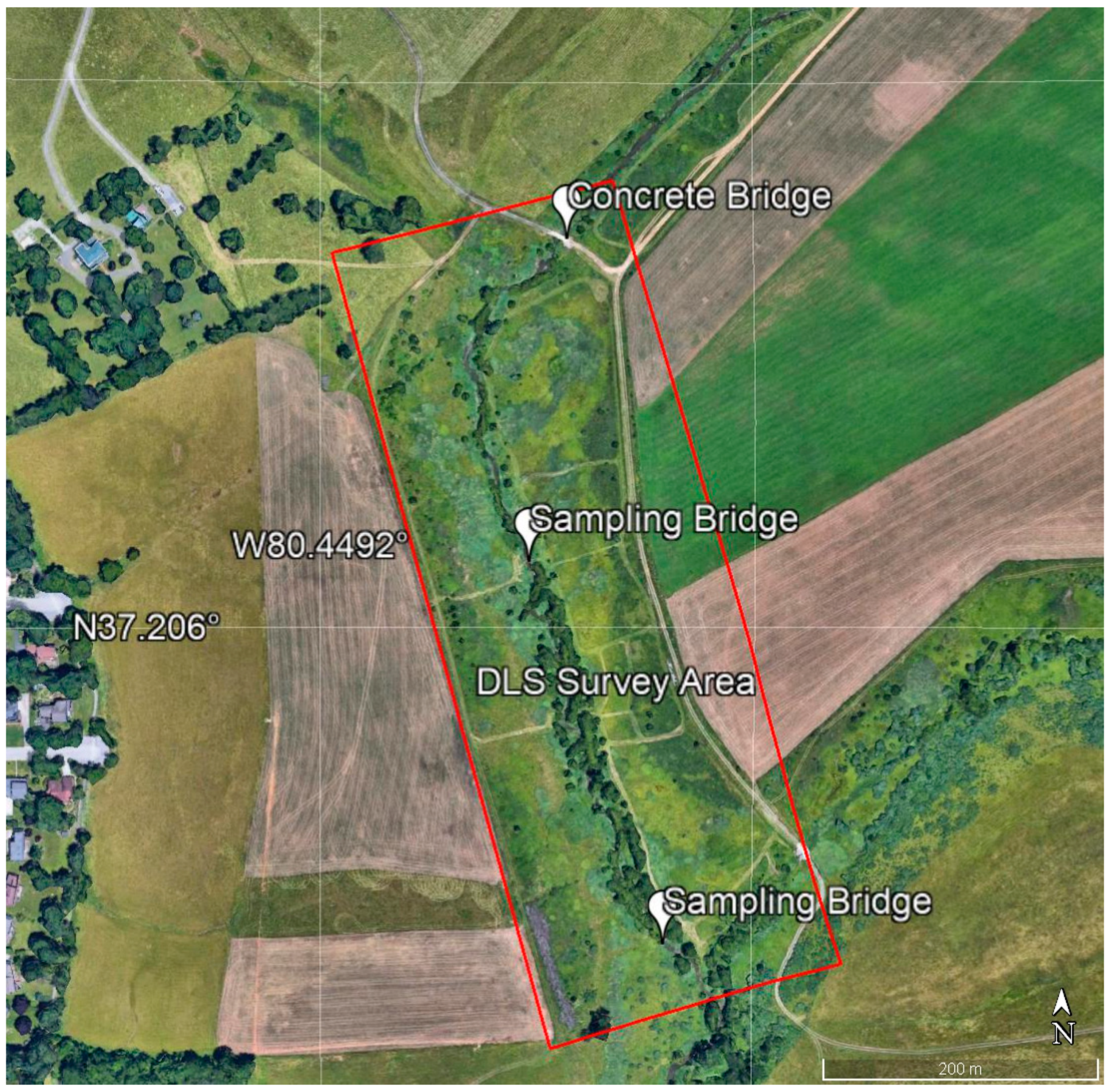
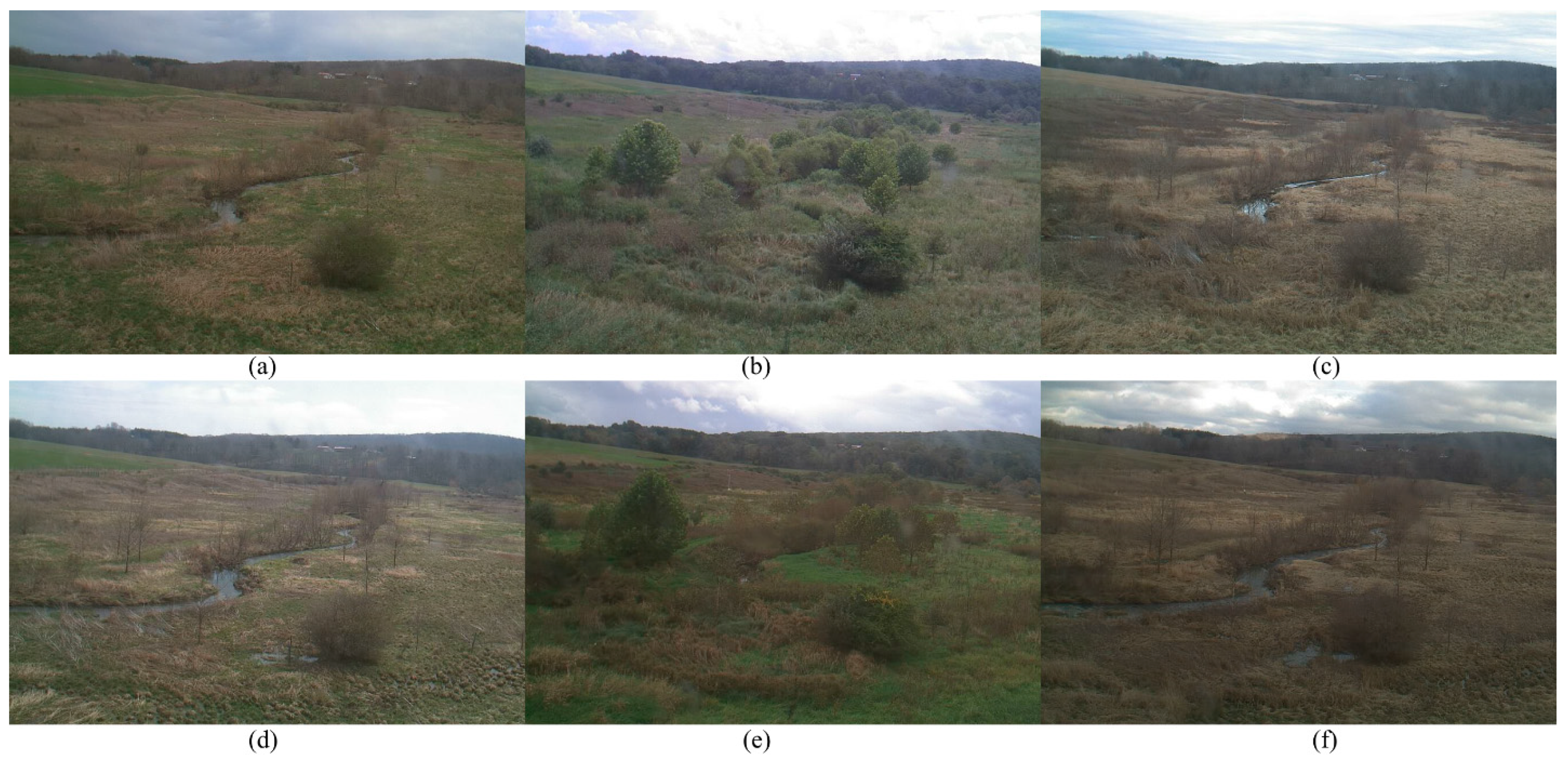
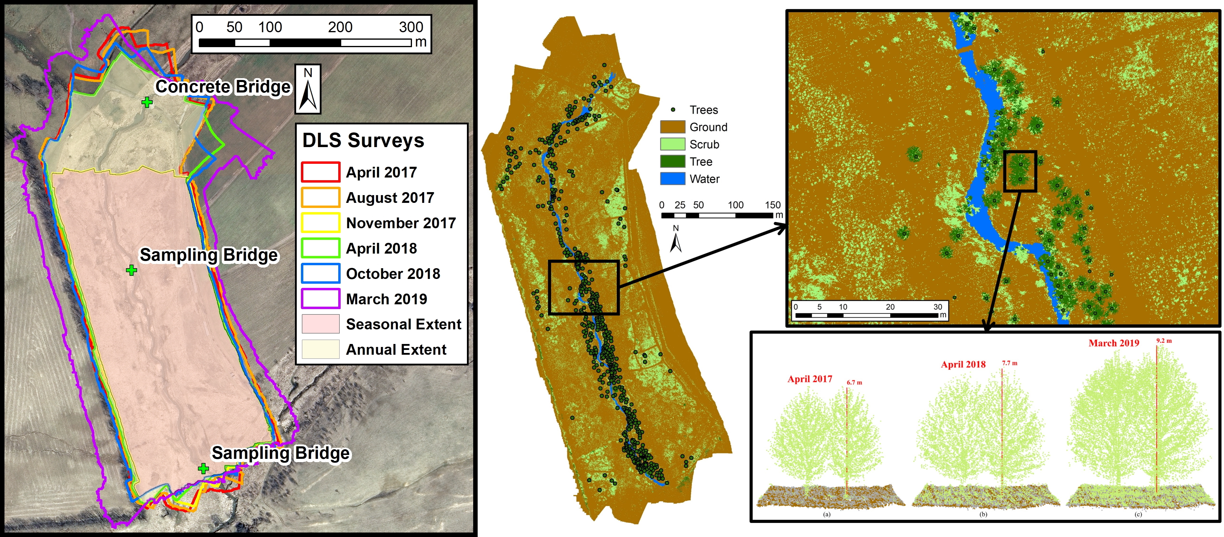
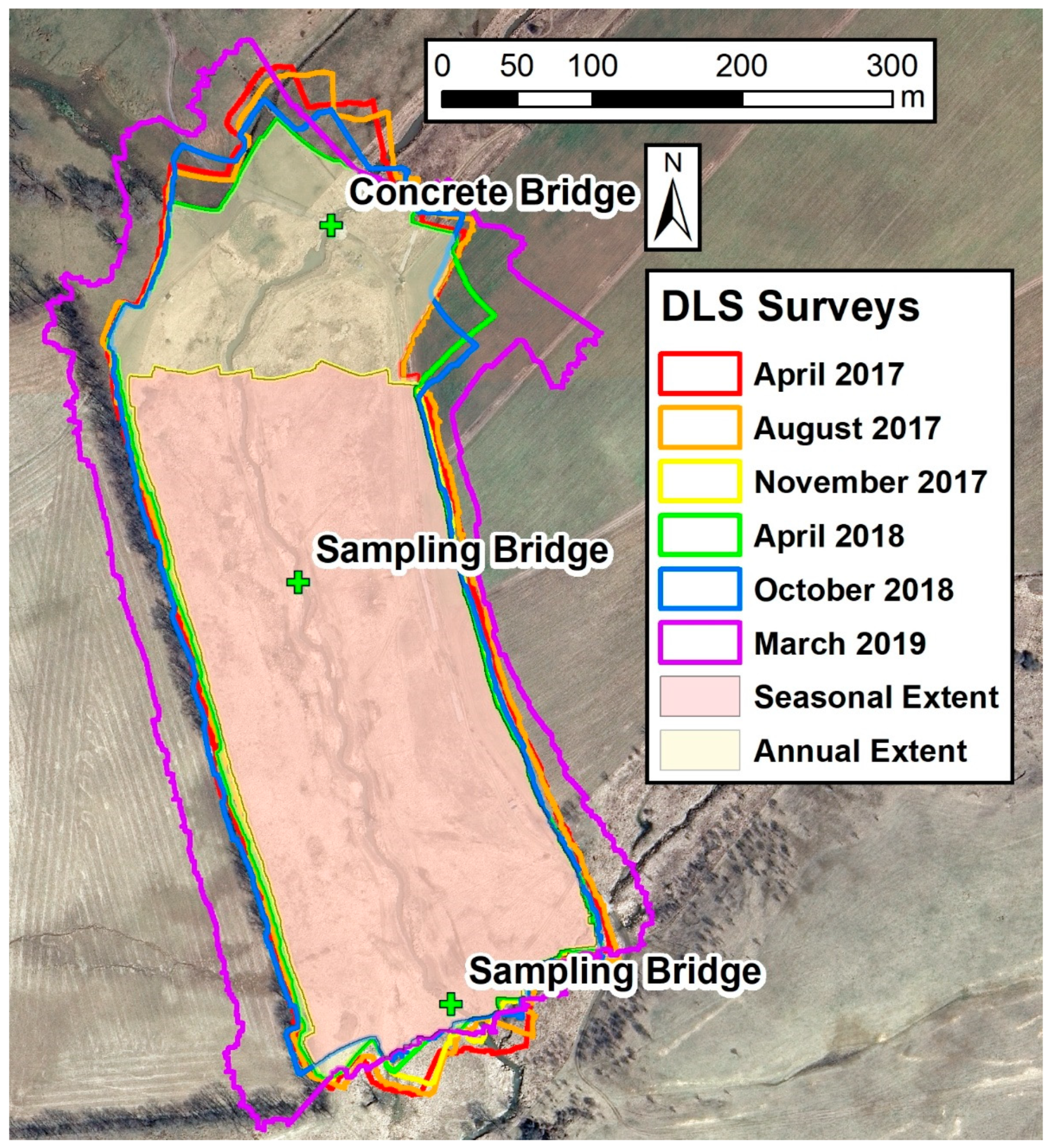
2.1. Study Area

The study area was a 0.65 km reach of Stroubles Creek located in Blacksburg, VA, USA (Figure 1). This reach has a history of agricultural use and underwent a stream restoration that was completed in May 2010 [33]. The restoration consisted of best management practices such as livestock exclusion, bank reshaping, and riparian vegetation planting [33]. The Stream Research, Education, and Management (StREAM) Lab at Virginia Tech continuously monitor water quality, stream flow, and weather at sampling bridges located along the reach as part of ongoing research efforts [34]. Resop and Hession [13] monitored streambank retreat on an 11 m bank of this reach using TLS between 2007 and 2009 and found that TLS was more accurate than traditional surveying methods for measuring topographic change; however, the stationary nature of TLS limited the study to a single streambank and was not ideal for larger extents. Resop et al. [9] scanned multiple streambanks and the floodplain using DLS in 2017, demonstrating the potential of DLS to perform change detection over the entire riverscape. Prior et al. [31] used DLS and SfM data for this reach from 2018 to estimate hydraulic roughness based on vegetation height and velocity data.

2.2. Lidar Data Collection

The drone used for this study was an AeroVironment Vapor35 (Arlington, VA, USA). The lidar system on board was a YellowScan Surveyor Core (Saint-Clément-de-Rivière France). The drone weighed approximately 13.6 kg with a payload (i.e., the lidar system) of about 2.3 kg. The battery provides a practical maximum flight time of 40 min at an altitude of 20 m above ground level (AGL). The lidar operated with a pulse rate of 300 kHz, used a near-infrared (NIR) wavelength of 905 nm and recorded up to two returns per pulse. Additional technical details for the drone and lidar systems can be found in Resop et al. [9], which used the same system to compare DLS and ALS for the same study area.

The reach was scanned six times over two years: 5 April 2017, 2 August 2017, 9 November 2017, 3 April 2018, 9 October 2018, and 20 March 2019. Three scans occurred during the leaf-off dormant vegetation season (April 2017, April 2018, and March 2019) and three scans occurred during the leaf-on season at varying stages of foliage (August 2017, November 2017, and October 2018; Figure 2). The extent was mostly similar for all six scans (Figure 1). Each flight consisted of six flightlines and accounted for overlap between swaths. All scans flew at a consistent altitude (about 20 m AGL), launch location, and speed to produce similar point densities, with the exception of the March 2019 scan, which tested a higher pulse density.

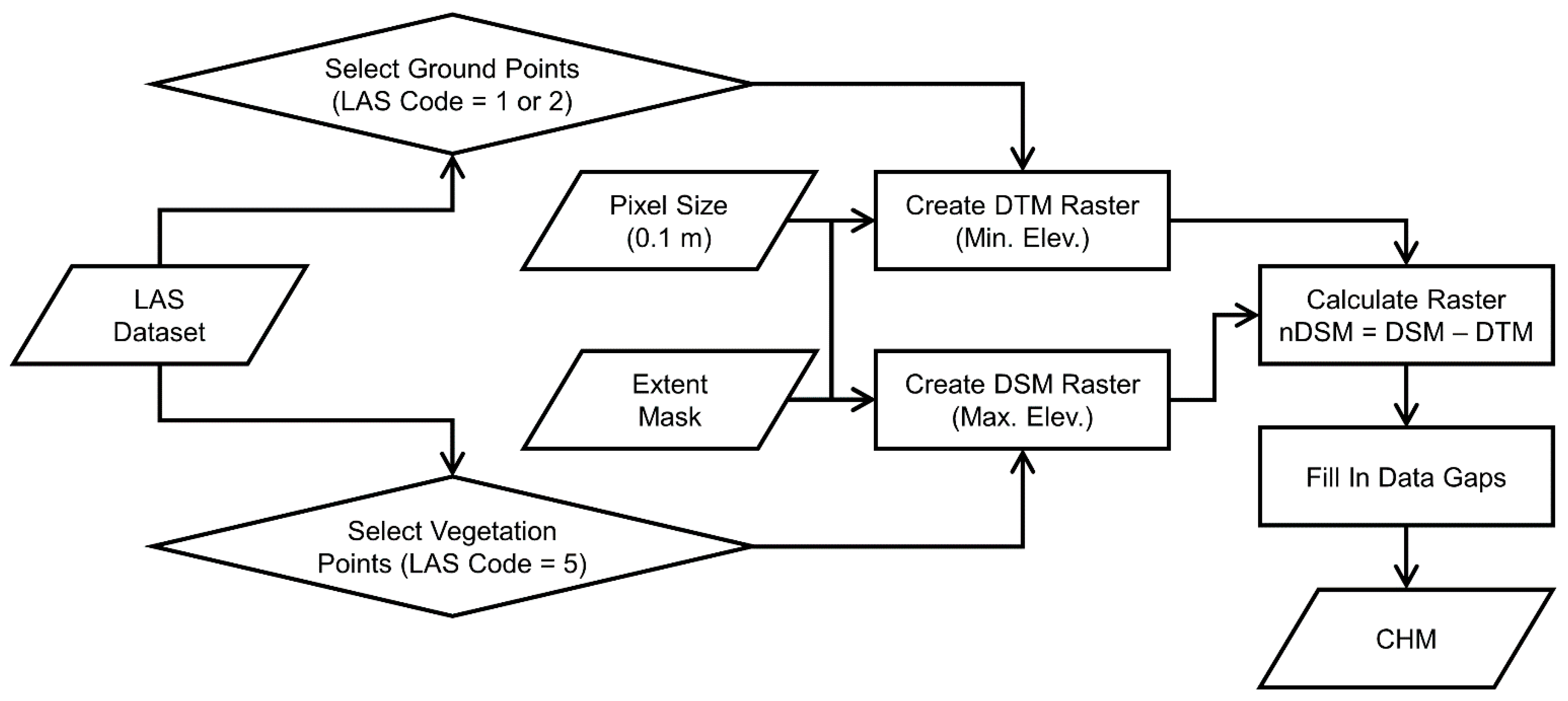
2.3. Lidar Data Preprocessing

The lidar data were georeferenced with the on-board GPS and local National Geodetic Survey CORS base station data [9]. For each scan, the DLS data was processed into six LAS files, one for each swath. The LAS files for each scan were added to a LAS dataset, projected to WGS 1984 UTM Zone 17N, and further classified and rasterized with ArcGIS 10.6 (Redlands, CA, USA) and LAStools (Gilching, Germany). Data analysis and visualization were performed with Python 3.7.7 and various open-source modules (e.g., numpy, pandas, matplotlib, sklearn).

The study area contained three prominent structures that served as control points to compare the DLS point clouds between scans: one concrete bridge used for vehicles at the north end of the reach and two wooden sampling bridges in the middle and south end of the reach (Figure 1). For each scan, lidar points representing bridges were manually classified as building with ArcGIS. Points representing other anthropogenic features (e.g., cars and people conducting the flights) were also classified as building so they would be ignored in further analysis.

During point cloud post-processing and georeferencing, an issue of concern occurred—some LAS files were not properly aligned with respect to the others. Two misalignment phenomena were observed: (1) within each scan, one of the six LAS files might be misaligned with respect to the other five, and (2) between each of the six scans, there might be an elevation bias. This issue was easily observed at bridges, which made it appear as if there were multiple bridges at the same location (Figure 3).

Misaligned LAS files were corrected with the open-source software CloudCompare 2.10 (https://www.cloudcompare.org/ accessed on 2 July 2021). A two-stage process was used: (1) within each scan to correct misaligned LAS files and (2) between each scan and the April 2017 baseline scan to correct bias. The three bridges were used as control points during alignment. Points were finely registered with the “Iterative Closest Point (ICP)” tool to a root mean squared difference (RMSD) of 0.00001 m and a transformation matrix was calculated. The transformation matrix was then applied to the entire point cloud. After correcting all six scans, the elevation bias was calculated between all scans and the April 2017 baseline scan as a measure of relative accuracy.

The extent of each lidar scan was delineated with ArcGIS [9]. The “LAS Point Statistics as Raster” tool created a 0.1-m raster representing all pixels with at least one point. The “Expand” and “Shrink” tools performed a morphological closing and removed small data gaps. The final raster was converted to a polygon representing the scan extent. Key differences in extents include the November 2017 scan, which had a smaller extent south of the concrete bridge, and the March 2019 scan, which had a larger extent expanding out into the floodplain (Figure 4). The extent intersection was calculated with the “Intersect” tool to normalize comparisons between scans. The “annual extent intersection” (between April 2017, April 2018, and March 2019) was 11.02 ha and the “seasonal extent intersection (between all scans) was 8.29 ha (Figure 4).

2.4. Lidar Data Classification

With respect to the lidar data collected for this study, noise was rare and most likely represented data artifacts, such as “bird hits.” The “Classify LAS Noise” tool in ArcGIS identified outlier points based on absolute minimum and maximum elevation thresholds. Afterwards, the point clouds from each scan were inspected with the “Profile View” tool and any remaining outliers were manually classified as noise.

After manually classifying building and noise, automated classification tools in ArcGIS were used to classify ground and vegetation points [9]. The “Classify LAS Ground” tool identified ground and “Classify LAS by Height” classified the remaining points as unassigned or vegetation based on a height threshold of 0.1 m (

Table 1. Lidar point data classes used in this study.

Class	Definition
Ground	Points most likely representing bare earth topography
Unassigned	Points between 0 m < height above ground < 0.1 m
Vegetation	Points between 0.1 m < height above ground < 15 m
Building	Points identified as human-made or built structures (e.g., bridges or cars)
Noise	Points identified as noise (e.g., bird-hits or lidar artifacts)

). Points with a height greater than 0.1 m were classified as vegetation and points less than 0.1 m were classified as unassigned. The unassigned class served as a measure of uncertainty, as these points were within the precision of DLS [35] and could represent ground or vegetation.

Researchers have observed that point clouds from a YellowScan lidar, which is based on the Velodyne Puck (San Jose, CA), can result in a “thickness” of points of a few centimeters when scanning flat ground, producing surfaces that are not as “crisp” as they should [36]. This phenomenon was observed in the point clouds produced for this study. Upon investigation, a cross-section of points along the concrete bridge at the northern end of the study area showed an approximate 0.05 m thickness of what should have been a solid surface. To account for this thickness, the unassigned class, representing points with a height above ground less than 0.1 m, was used in addition to the ground class to define terrain for bare earth models (i.e., DTMs).

The automated classification algorithms produced two common misclassifications: (1) ground points misclassified as vegetation on high-gradient stream banks and (2) vegetation points misclassified as ground under dense canopy [9]. These misclassifications need to be corrected manually due to limitations in current lidar point classification algorithms. Unfortunately, the manual correction of large point clouds, especially from DLS, is very time-consuming and labor-intensive [9]. The April 2017 scan was corrected previously [9], but the other five scans were not fully verified. An investigation into a more efficient classification correction process was outside the scope of this study.

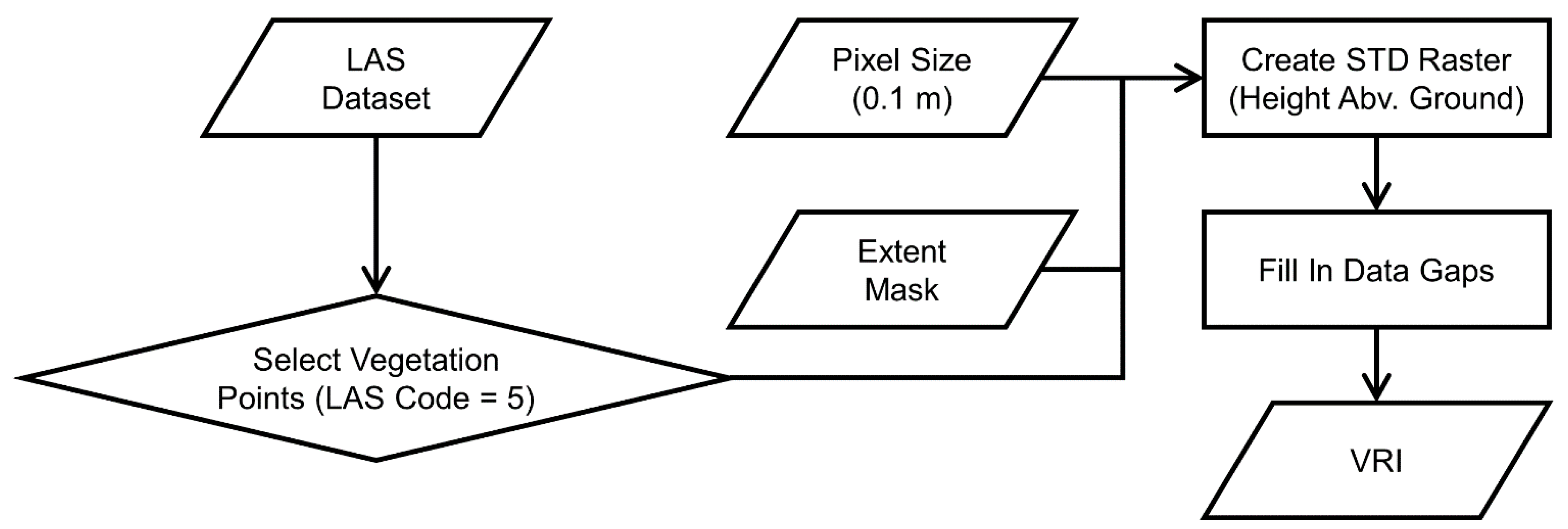
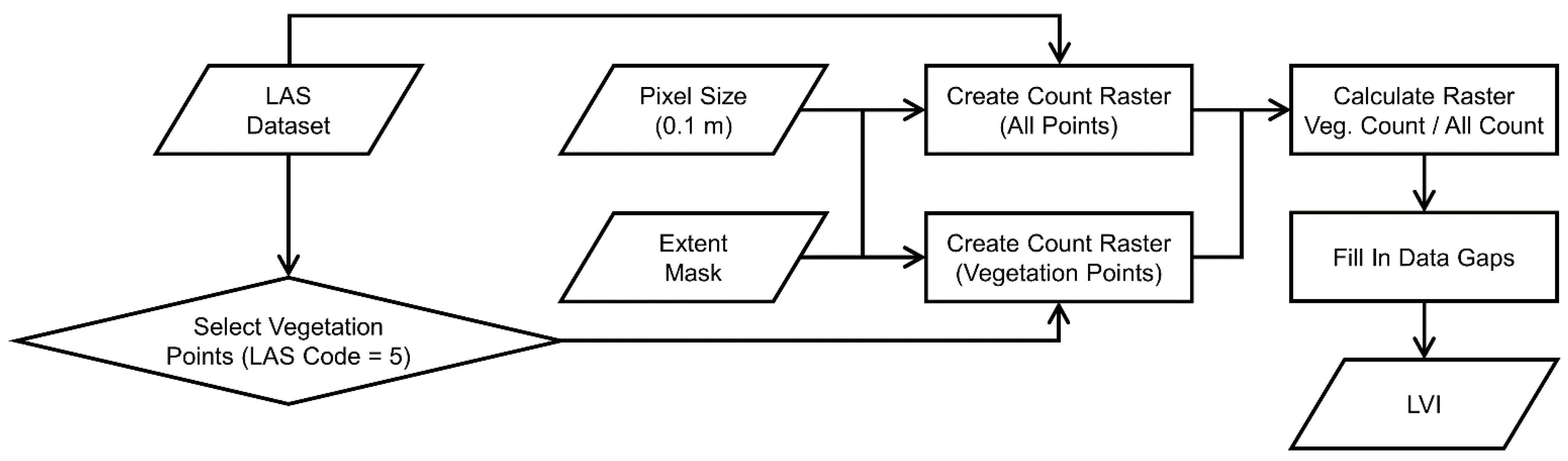
2.5. Lidar Vegetation Metrics

Three lidar metrics were selected to represent riverscape vegetation: (1) height (canopy height model; CHM), (2) roughness (vegetative roughness index; VRI), and (3) density (lidar vegetation index; LVI;

Table 2. Metrics produced from drone laser scanning (DLS) data to represent different components of riverscape vegetation.

Lidar Vegetation Metrics	Definition	Value Range	Units
Canopy height model (CHM)	Measure of vegetation height (veg. elev.) − (ground elev.)	0 to ~13	Meters
Vegetative roughness index (VRI)	Measure of vegetative roughness St. dev. of vegetation height	0 to ~9	Meters
Lidar vegetation index (LVI)	Measure of vegetation density (count veg.)/(count all points)	0 to 1	Decimal Percent

). All three metrics were calculated in raster format for each DLS survey using data processing pipelines created with Model Builder in ArcGIS. All outputs had a pixel size of 0.1 m. Based on an average point spacing of 0.047 m over the six scans, this is about five lidar points per pixel.

The CHM was derived from two rasters: the DTM (i.e., the minimum ground and unassigned point elevation per pixel) and the DSM (i.e., the maximum vegetation point elevation per pixel) [9]. The DTM and DSM were calculated with the “LAS Dataset to Raster” tool (Figure 5). The difference between DSM and DTM resulted in a normalized digital surface model (nDSM) [9]. Data gaps (e.g., water surfaces and lidar shadows) and pixels with a height less than 0.1 m (i.e., the smallest height of vegetation points), were assigned zero values to produce the final CHM. The CHM ranged from 0 m (i.e., bare earth) to about 13 m (i.e., the height of the tallest tree).

The vegetative roughness index (VRI) estimated the local variability of vegetation height. The VRI was calculated with the “LAS Height Metrics” tool as the standard deviation of vegetation point height per pixel (Figure 6). Points with a height less than 0.1 m were ignored. Low standard deviations corresponded to smooth surfaces while high standard deviations corresponded to rough surfaces. Data gaps were assigned a VRI of zero. The VRI ranged from about 0 m, representing relatively uniform vegetation, to 9 m, representing more complex vegetation.

The lidar vegetation index (LVI) represented the percentage of vegetation points per pixel. While CHM and VRI were both absolute measures, the LVI was the only relative measure. The number of vegetation points per pixel was calculated with the “LAS Point Statistics as Raster” tool and then the number of total points per pixel was calculated (Figure 7). The vegetation point count was divided by the total point count on a pixel-by-pixel basis, resulting in a decimal percentage. Data gaps were assigned an LVI of zero. The LVI ranged from zero, representing no vegetation or open canopy, to one, representing heavy vegetation or dense canopy.

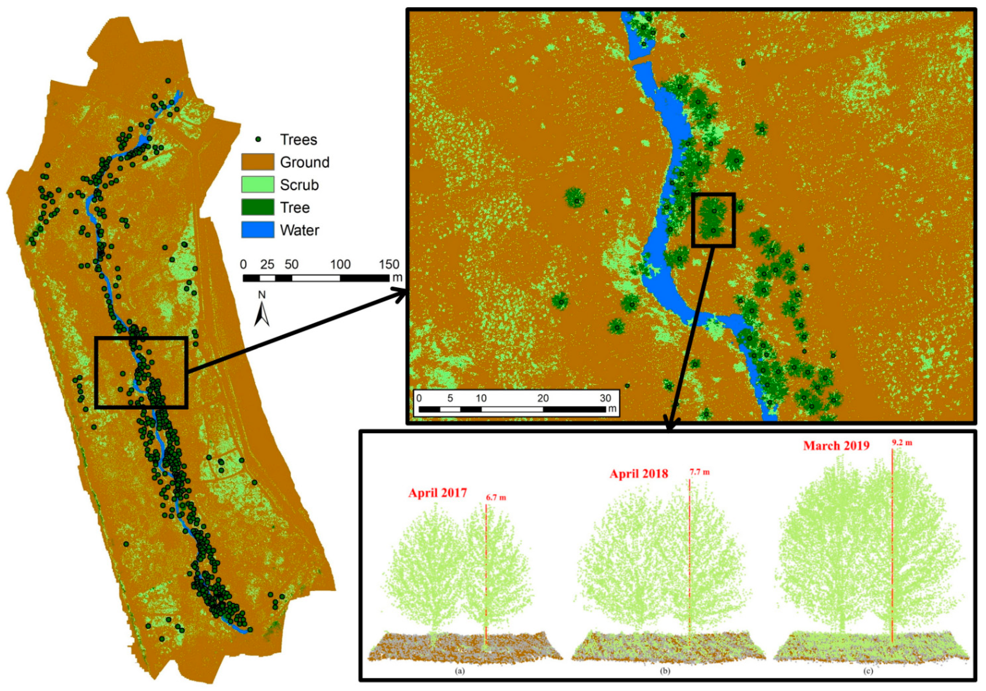
2.6. Vegetation Classification, Distance to Water, and Tree Identification

The CHM for each scan was classified into the following land classes: ground, scrub, and tree. These classes were defined with a simple threshold method based on a manual investigation of vegetation in the riverscape. Pixels with a CHM value (i.e., height above ground) less than 0.1 m were classified as ground, pixels between 0.1 and 2 m were classified as scrub, and pixels greater than 2 m were classified as tree.

The CHM for the April 2017 baseline was used to establish the stream location. A land class for water was defined by taking advantage of the physics of NIR lidar pulses, which are absorbed by water surfaces and result in “No Data” pixels. The “LAS Point Statistics as Raster” tool counted the lidar points in each 0.1 m pixel and those with more than three points represented ground. The “Expand” and “Shrink” tools were used to close small data gaps. At this point, “No Data” gaps represented the water surface. Once the water class was defined, the “Euclidean Distance” tool was used to determine the distance between each pixel in the riverscape and the stream.

To quantify the annual growth of vegetation, trees were manually identified from the April 2017 CHM based on pixels classified with a height greater than 2 m. The riverscape was inspected, crowns were identified, and stems were marked. The environment for this study had a fairly open canopy, so it was easy to manually identify trees. Each identified tree was verified by inspecting the point cloud. The “Buffer” tool created 0.5 m buffers around each tree stem and the maximum tree height was calculated from the CHMs for April 2017, April 2018, and March 2019.

2.7. Annual and Seasonal Change Detection

Annual and seasonal changes were calculated for each vegetation metric (Table 2). The overall two-year period was represented by the April 2017 to March 2019 scans. Annual change was measured between leaf-off scans (April 2017 to April 2018 and April 2018 to March 2019) within the annual extent intersection (Figure 4). Seasonal change was measured between all six DLS scans within the seasonal extent intersection (Figure 4).

An effective method of identifying pixel-level change is to calculate DEMs of difference (DoDs) by subtracting rasters representing two moments in time: the newer raster minus the older raster [12,37,38]. For CHMs, change represented vegetation growth or decay [15]. For VRIs, change represented increased roughness or smoothness. For LVIs, change represented increased or decreased vegetation density. Change was determined to be significant, as opposed to noise, by applying a minimum level of detection (LoD), representing the uncertainty of the lidar sensor [37,38]. An LoD of 0.05 m was used for the CHM and VRI DoDs [35], which is consistent with LoDs used by change detection studies involving lidar at a similar range [17]. For the LVI DoD, the unassigned class (Table 1) represented the point classification uncertainty.

3. Results

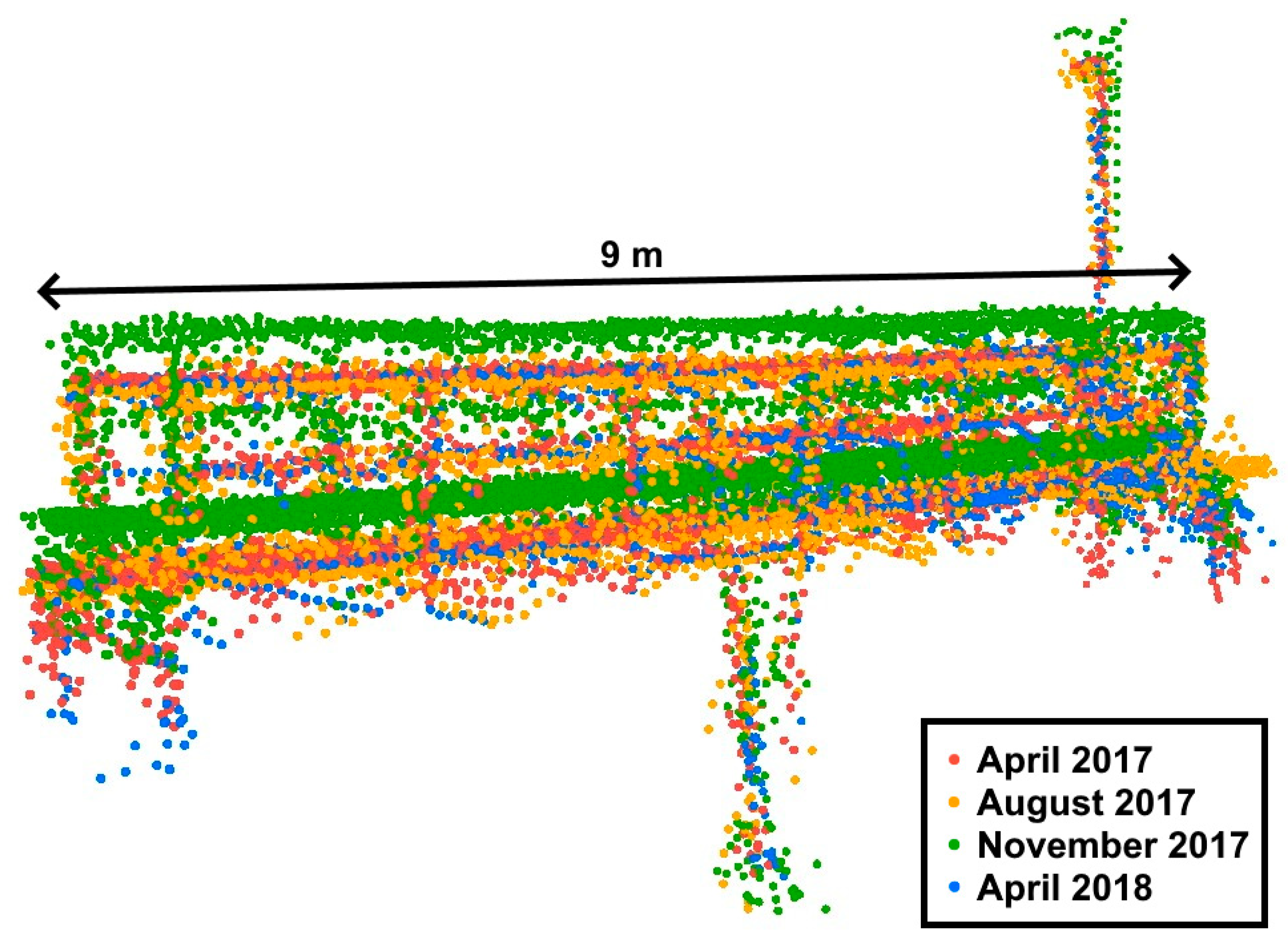
3.1. Point Density Comparison and Elevation Bias between the Six Lidar Scans

The point count varied significantly between the scans due to extent differences (Figure 4), ranging from 42.6 to 70.1 million points. When considering only the seasonal extent intersection the point counts were more consistent (

Table 3. Drone laser scanning (DLS) statistics for each scan within the extent intersection.

Scan Date	Point Count	Point Density (All Returns/m2)	Pulse Density (First Returns/m2)
April 2017	41,661,008	502.43	492.39
August 2017	42,148,141	508.30	501.89
November 2017	42,389,739	511.21	490.65
April 2018	42,994,259	518.51	501.61
October 2018	42,584,883	513.57	500.07
March 2019	51,135,652	616.69	590.30

). Most scans contained between 41.7 and 43.0 million points with the exception of the March 2019 scan, which contained 51.2 million points due to a higher pulse density. While most scans were consistent (491 to 502 pulses/m²), the March 2019 scan had a pulse density of 590 pulses/m².

Agreement between the six DLS scans was determined based on the average elevation (Z) bias between DEMs produced from each scan and the April 2017 baseline. Bridge DEMs were created using points representing the concrete bridge and two sampling bridges. Before aligning the data in CloudCompare, the average Z bias was as large as 1.15 m (March 2019) with smaller biases of 0.23 m (November 2017) and −0.11 m (October 2018; Figure 3). After alignment, the average Z biases ranged from−0.03 m to 0.01 m over all six scans (

Table 4. The average elevation (Z) bias between each drone laser scanning (DLS) survey and the April 2017 scan after all point clouds were aligned with CloudCompare.

Scan Date	Mean Z Bias (m) Bridge DEMs	Mean Z Bias (m) Ground DTMs
April 2017	Baseline	Baseline
August 2017	−0.02	0.25
November 2017	−0.01	0.06
April 2018	0.01	−0.01
October 2018	−0.02	0.17
March 2019	−0.03	−0.03

), which is well within the precision of YellowScan lidar systems [35].

Between DTMs, the average Z biases had a wider range, −0.03 m to 0.25 m (Table 4). The scans with a higher bias included August 2017 (0.25 m), October 2018 (0.17 m), and November 2017 (0.06 m), which occurred during leaf-on seasons. The Z bias was negatively correlated to the time of year. Going forward in time from August to October to November, as the amount of vegetation decreased there was a lower likelihood of vegetation understory misclassified as ground, which decreased the bias. For the other leaf-off scans (April 2018 and March 2019), the bias was within the precision of the lidar system (−0.01 m and −0.03 m, respectively) [35].

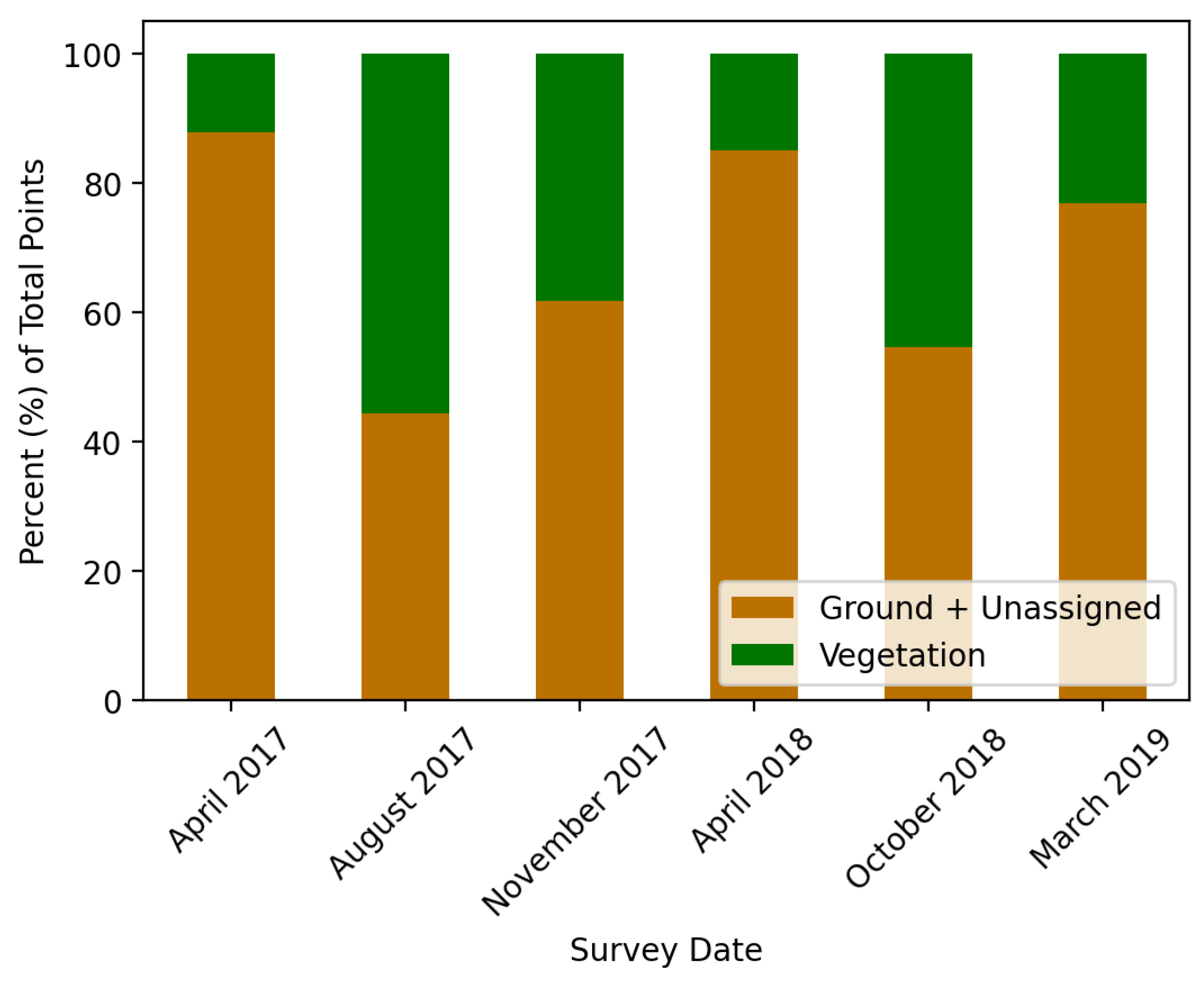
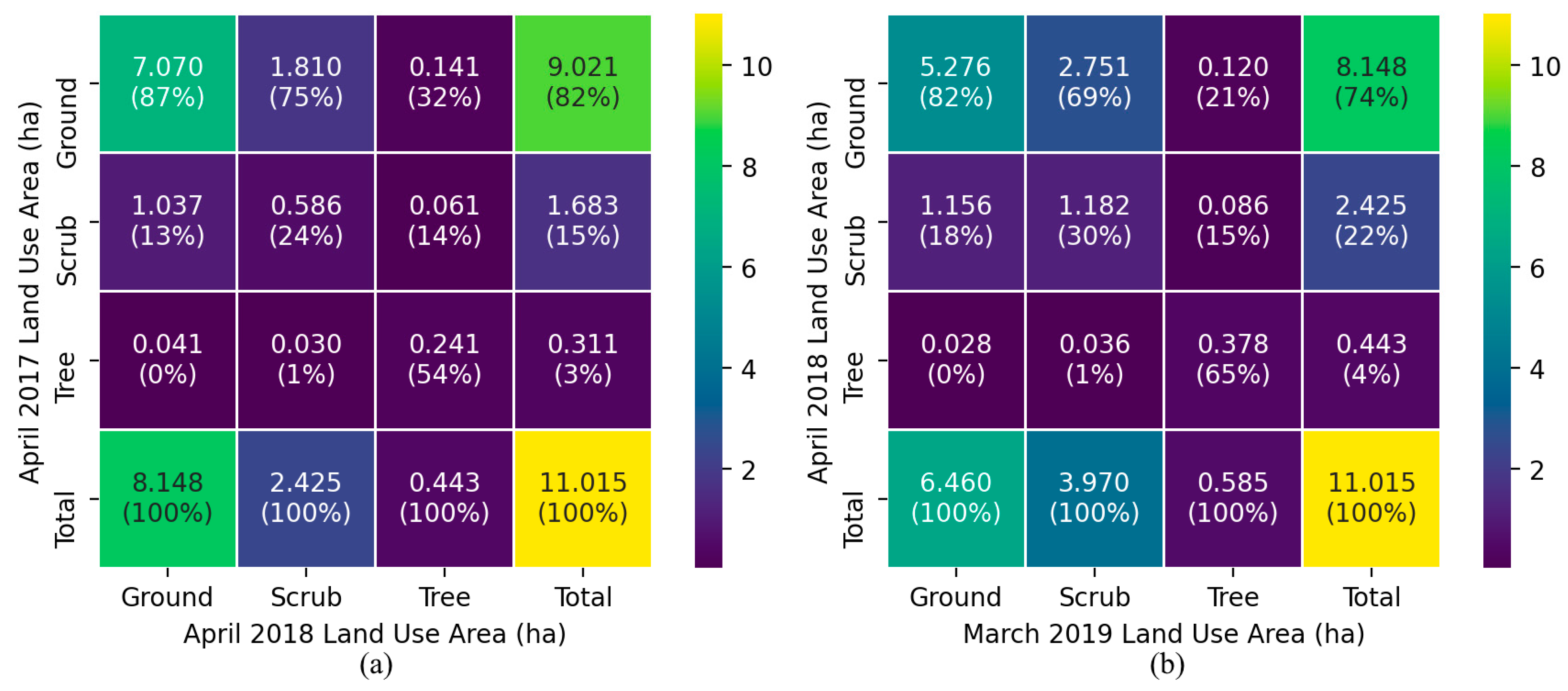
3.2. Annual and Seasonal Change of Lidar Point Classifications

The three primary data classes were ground, unassigned, and vegetation (Table 1). Vegetation represented objects with a height above ground greater than 0.1 m that were not identified as a built structure, which allowed DLS to detect not just trees and bushes but also small herbaceous vegetation [9]. The scans were clipped to the seasonal extent intersection and the point statistics (percent terrain vs. percent vegetation) were compared. As expected, the percent vegetation varied periodically throughout the seasons as associated with the growth and decay of vegetation in the riverscape, with a maximum of 56% in August 2017 (leaf-on) and a minimum of 12% in April 2017 (leaf-off; Figure 8). During the leaf-on scans, there was a clear negative trend in the percent vegetation going forward in time from August (56%) to October (45%) to November (38%), likely due to the decay of leaves over the autumn season.

There was a gradual increase in percent vegetation over time between the leaf-off scans going forward in time from April 2017 (12%) to April 2018 (15%) to March 2019 (23%; Figure 8). This positive trend was likely reflecting the annual growth of vegetation in the riverscape. The higher pulse density during the March 2019 scan (Table 3) may have contributed to the higher percent vegetation observed for this scan, but the level of influence is not clear.

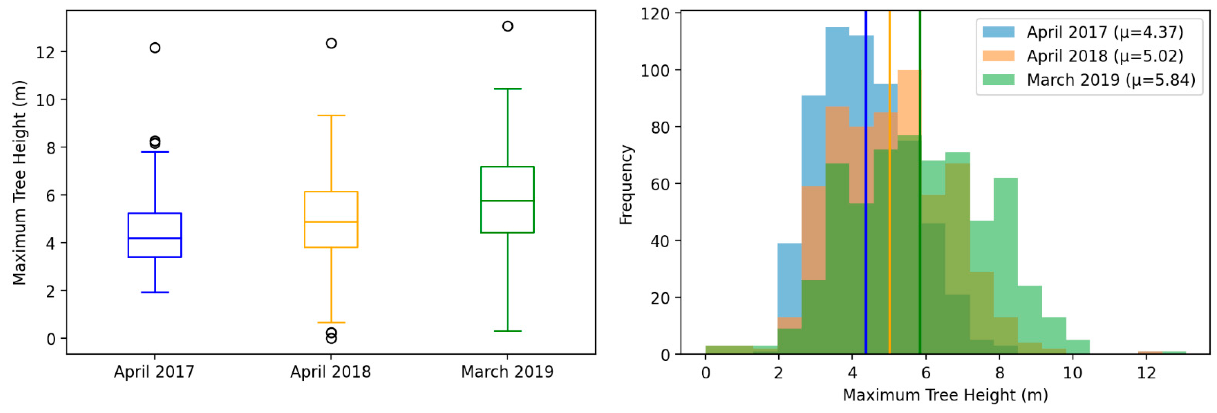
3.3. Annual Change of Maximum Tree Height

A total of 604 trees were identified in the April 2017 CHM based on a manual inspection of areas classified as tree (CHM > 2 m; Figure 9). The average tree growth over the two-year period was 1.48 m. A majority of trees had positive growth (n = 570; mean = 1.62 m) while a few had negative growth (n = 34; mean = −0.96 m). Most trees with negative growth fell due to natural causes over the two-year period. Tree growth was greatest from 2018 to 2019 (mean = 0.83 m) compared to the period 2017 to 2018 (mean = 0.65 m). Based on the tree’s distance to stream (i.e., pixels classified as water), trees within 20 m grew faster (n = 544; mean = 1.56 m) over the two-year period compared to trees farther than 20 m (n = 60; mean = 0.70 m).

Not only did the trees show steady average growth (April 2017 = 4.37 m, April 2018 = 5.02 m, March 2019 = 5.84 m), but the variability or standard deviation of height increased over time as well (April 2017 = 1.28 m, April 2018 = 1.58 m, March 2019 = 1.90 m). This positive trend in standard deviation demonstrates not just an increase in tree height over time but also tree height diversity and variability (Figure 10). Overall, the annual scans showed a consistent, steady growth of woody vegetation over the riverscape.

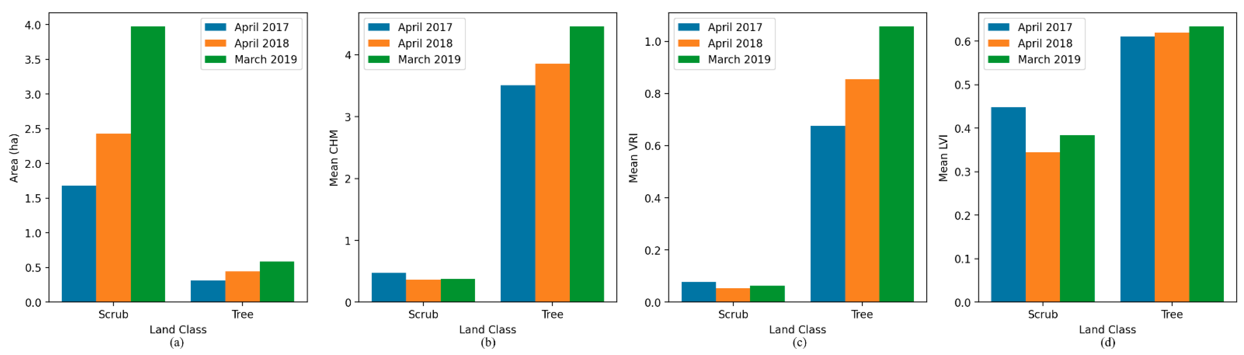
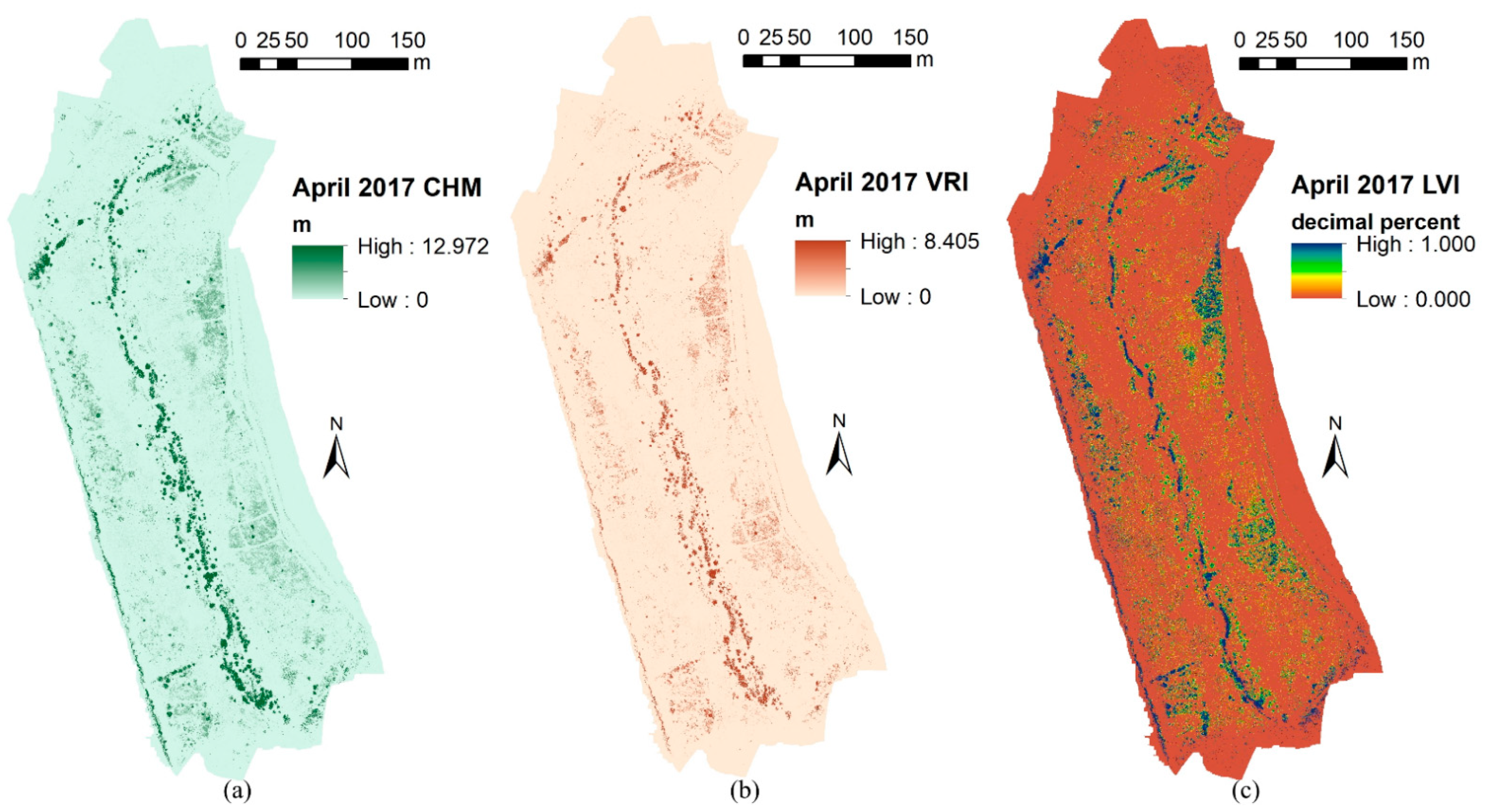
3.4. Baseline Lidar Vegetation Metrics

The vegetation metrics (CHM, VRI, and LVI) were derived for the April 2017 scan as a baseline (Figure 11). The CHM ranged from 0 m (bare ground) to 12.97 m (the height of the tallest tree). The VRI ranged from 0 m (smooth surfaces) to 8.41 m (rough surfaces). The LVI ranged from 0 (open terrain) to 1 (dense vegetation). The April 2017 scan was classified as: ground (CHM < 0.1 m), scrub (0.1 m < CHM < 2 m) and tree (CHM > 2 m; Figure 9). As expected, pixels classified as ground had a value close to zero for all three metrics. For pixels classified as vegetation, tree areas consistently had higher vegetation metrics than scrub areas. The biggest difference was between average height (CHM; scrub = 0.48 m and tree = 3.52 m), which is to be expected since the classes were determined based on height. The differences between roughness (VRI; scrub = 0.08 m and tree = 0.67 m) and density (LVI; scrub = 0.45 and tree = 0.61) were much smaller.

Very weak negative correlations were observed between CHM (R² = 0.12) and VRI (R² = 0.07) with respect to the distance to the stream channel, but overall the taller and rougher vegetation tended to be located closer to the stream (Figure 12). There was no correlation between LVI (R² = 0.01) and distance to stream; however, it is important to note that within the stream channel itself the LVI ~ 1 due to the fact that the water surface absorbed the lidar pulses resulting in a lack of ground points measured by the lidar system (Figure 11).

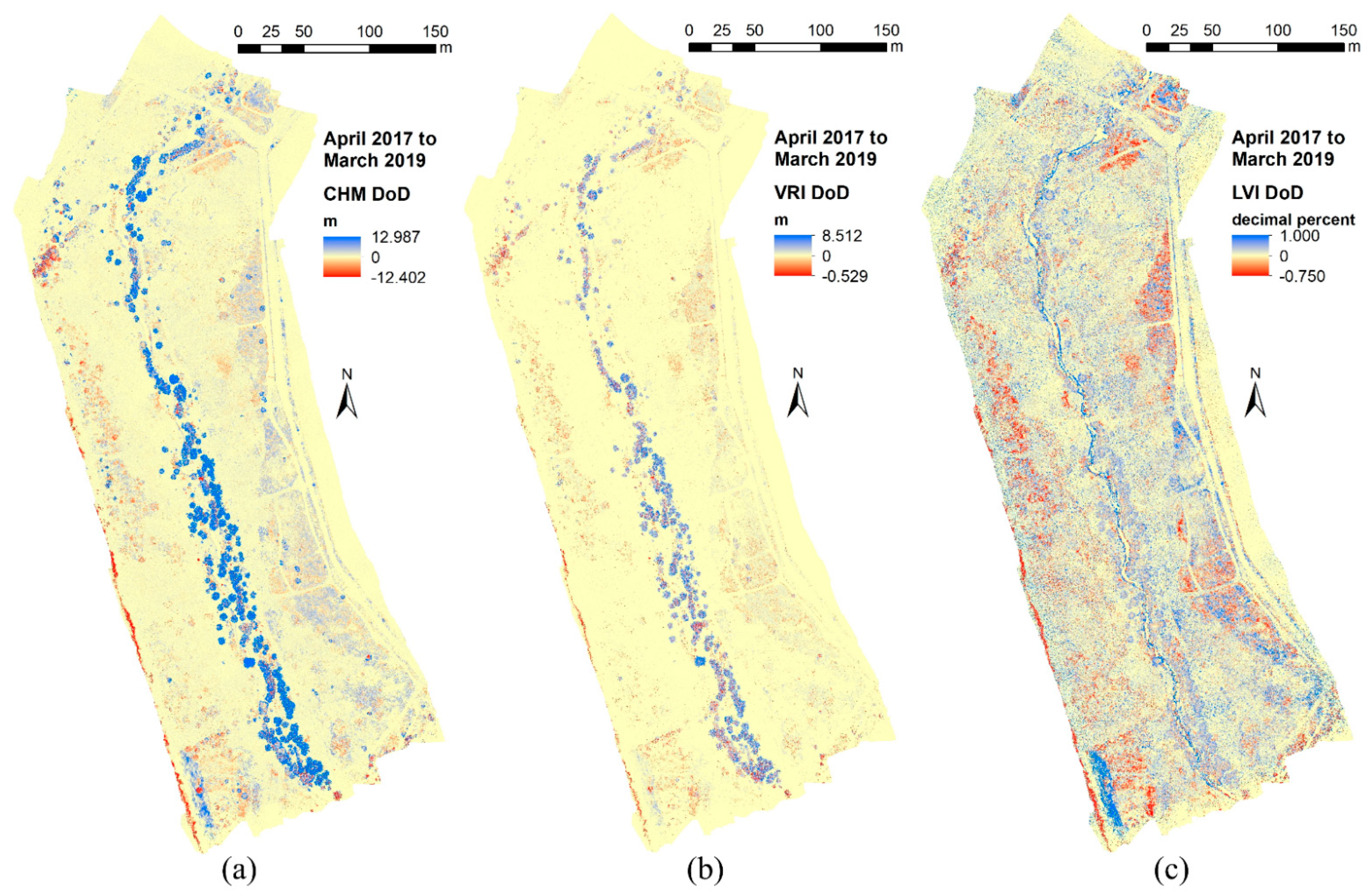
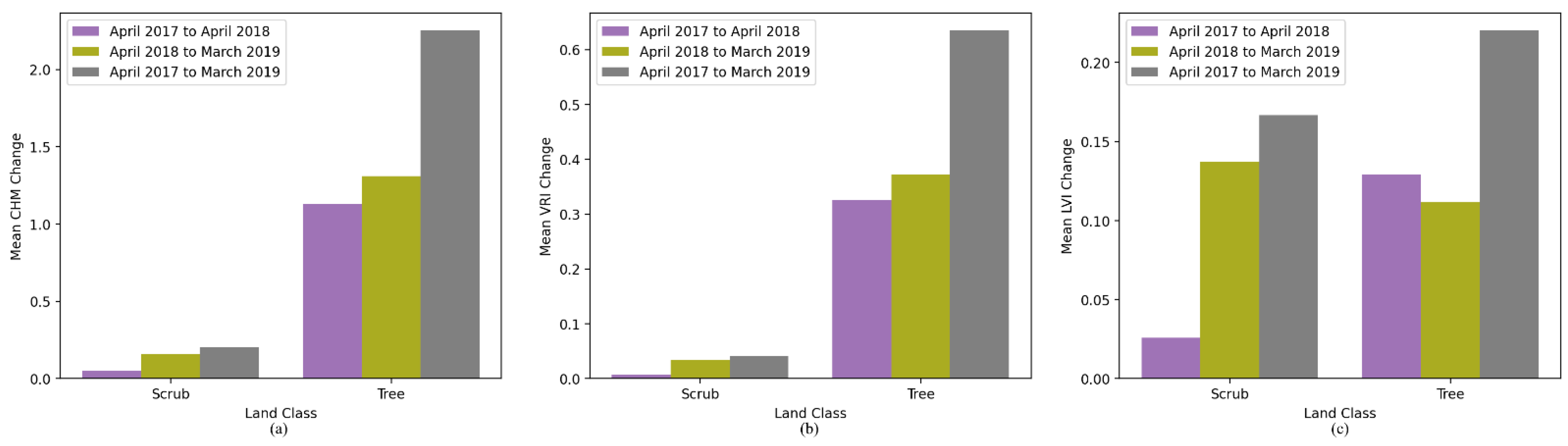
3.5. Annual Change of Lidar Vegetation Metrics

The vegetation metrics for the annual leaf-off scans (April 2017, April 2018, and March 2019) were overlaid with each vegetation class (scrub and tree) and clipped to the annual extent intersection (total area = 11.02 ha). Both scrub and tree areas increased steadily over the two-year period (Figure 13). Scrub, as a percent of the total area, increased from 15.28% for April 2017 to 22.02% for April 2018 to 36.04% for March 2019 while tree area increased from 2.83% to 4.02% to 5.31%. In tree areas, all three metrics increased over the two-year period (Figure 13). An increase in height (CHM) was driven by annual tree growth (Figure 10). However, increases in roughness (VRI) and density (LVI) were likely also influenced by the growth of understory. On the other hand, scrub areas did not show any significant annual trends with respect to any metric (Figure 13). Annual variations in scrub vegetation were likely impacted by the growth of new scrub and decay of old scrub, while trees had more consistent growth without much change in the overall tree population.

There was a clear increase in total scrub and tree area over each year (Figure 13). By looking at the 0.1 m pixel-level change, one can investigate how land class changed from one year to the next. From April 2017 to April 2018, scrub area increased from 1.68 ha to 2.43 ha; however, a majority (75%) of the April 2018 scrub area was previously ground (Figure 14) and a majority (62%) of the April 2017 scrub area became ground in April 2018. This same trend was observed between April 2018 and March 2019 when the scrub area increased from 2.43 ha to 3.97 ha and again a majority (69%) was previously ground (Figure 14) and a near majority (48%) of the previous scrub became ground. This demonstrates the volatility of scrub areas and could have dramatic effects on physical riverscape properties such as hydraulic roughness from year to year. In contrast, tree areas showed more consistency. From April 2017 to April 2018 to March 2019 the tree area increased from 0.31 ha to 0.44 ha to 0.59 m. Unlike scrub area, a majority of the tree area in both 2018 and 2019 was previously classified as tree, 54% and 65%, respectively (Figure 14).

Looking at the DoDs, one can observe the pixel-level growth and decay of vegetation spatially over the riverscape and temporally over the two-year study (Figure 15). The DoDs for height (CHM) and roughness (VRI) showed similar trends; although, the CHM had a greater overall magnitude of change compared to the VRI. Most of the positive change in vegetation occurred near the stream channel and was primarily due to the growth of trees. Farther into the floodplain, there was more spatial variability in the growth and decay of scrub. From year to year, some sections of scrub showed positive change and some showed negative change. Overall, tree areas showed greater growth in CHM and VRI over the two-year period compared to scrub areas (Figure 16). On the other hand, vegetation density (LVI) consistently had positive change over the entire riverscape (Figure 15) and the change was similar between scrub and trees (Figure 16). This consistent growth in vegetation density suggests that while scrub and trees are growing at different rates, the canopy density and vegetation understory is increasing more uniformly.

The vegetation metrics did not show much correlation with distance to stream. However, when selecting only tree areas, some annual trends were observed. There was a negative correlation for tree height and roughness with distance to stream (Figure 17). The negative correlation increased in magnitude over time from April 2017 to April 2018 to March 2019 (Figure 17). Generally, trees grew faster within 20 m of the stream compared to trees farther than 20 m. The average CHM growth from 2017 to 2019 was 1.03 m within 20 m and 0.07 m farther than 20 m. The average increase in VRI over the same period was 0.40 m within 20 m and 0.12 m farther than 20 m. While tree height and roughness showed a negative correlation with distance to stream, vegetation density showed a positive correlation over the two-year period (Figure 17). This positive correlation in tree areas decreased over time from 2017 to 2019 as the average LVI increased by +0.05 within 20 m but decreased by −0.09 farther than 20 m. Overall, the annual trend for all three metrics showed a greater increase in vegetation closer to the stream. While these annual trends were observed in tree areas, there were no significant correlations or trends observed in scrub areas. This is likely a result of the volatility of the scrub area over the riverscape that was previously described.

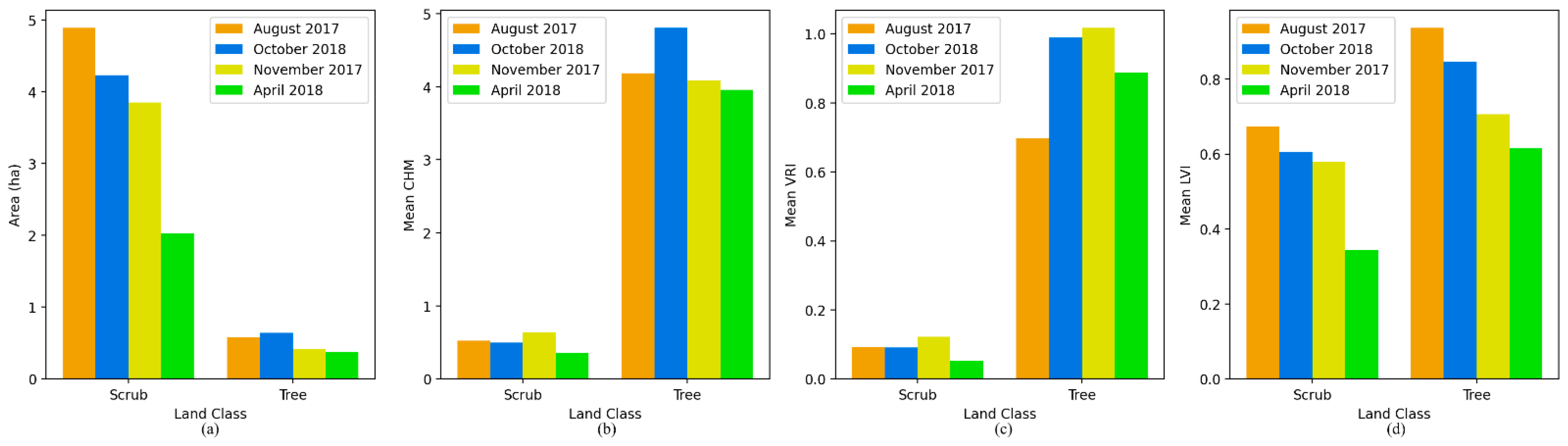
3.6. Seasonal Change of Lidar Vegetation Metrics

All six scans were clipped to the seasonal extent intersection (total area = 8.29 ha). Based on the change in vegetation area, two periods were associated with growth (April 2017 to August 2017 and April 2018 to October 2018) and three periods were associated with decay (August 2017 to November 2017, November 2017 to April 2018, and October 2018 to March 2019; Figure 18). These trends were similar to what was previously observed when looking at the classified lidar point clouds (Figure 8). Much like the observations of annual change for individual trees and the pixel-level change of the vegetation metrics, tree areas gradually increased in height (CHM) and roughness (VRI) over time (Figure 18). On the other hand, scrub areas were more constant for both metrics (Figure 18). Density (LVI) was highly variable for both scrub and trees (Figure 18).

Temporal linear regression was used to remove the annual trend of each metric for scrub and tree areas and isolate the seasonal variability, which was represented by the normalized root mean squared error (NRMSE) of the regression residuals (

Table 5. Regression results showing the annual trend (based on R²) and seasonal variability (based on normalized root mean squared error [NRMSE]) for each metric and land class.

	Scrub Land Class Areas		Tree Land Class Areas
Vegetation Metric	Annual Trend (R2)	Seasonal Variability (NRMSE)	Annual Trend (R2)	Seasonal Variability (NRMSE)
Height (CHM)	0.16	17.8%	0.70	5.1%
Roughness (VRI)	0.08	25.6%	0.70	9.2%
Density (LVI)	0.08	23.1%	0.00	17.8%

). Out of all the combinations of lidar metric and land class, only height and roughness in tree areas had significant annual trends (both had R² = 0.70). Both scrub and tree areas demonstrated seasonal variability for height and roughness; however, the variability was greater for scrub (CHM NRMSE = 17.8%; VRI NMRSE = 25.6%) compared to trees (CHM NRMSE = 5.1%; VRI NMRSE = 9.2%). Vegetation density did not have any significant annual trends. However, it was highly seasonally variable for both scrub areas (LVI NRMSE = 23.1%) and tree areas (LVI NRMSE = 17.8%).

No temporal trends could be observed for the average vegetation density (LVI) when viewing the data sequentially (Figure 18). However, by reordering the scans as they would fall in a single growing season, a trend emerges representing vegetation decay (Figure 19). The scans were reordered August (2017) to October (2018) to November (2017) to April (2018). This time shift does not work well for height and roughness since these are absolute measures and are affected by annual vegetation growth. On the other hand, density is a relative measure based on the local percentage of vegetation points. By reordering the scans seasonally, one can observe a negative trend in LVI over both scrub and tree areas (Figure 19). This trend likely represents the seasonal decay of vegetation in the riverscape as foliage falls and DLS is able to penetrate further through the canopy to record ground points.

4. Discussion

Limitations with the Current Study and Future Research

One of the limitations of raster-based analysis is that only a single Z value is allowed per pixel. When quantifying height or classifying different types of vegetation this limitation does not allow for an accurate representation of complex environments; in particular, when multiple vegetation types exist at the same location. For example, when grass or scrub grows under a tree canopy. With traditional image-based remote sensing, these distinctions are often impossible to make. However, since lidar can penetrate through the tree canopy, it is possible to derive lidar measures that represent this vegetation diversity. Many applications take advantage of this aspect of lidar data by generating metrics such as average height, standard deviation, point density, and height percentiles to represent forest structure [20]. The lidar metrics generated in this study, representing height, roughness, and density, allowed for different perspectives of vegetation structure. These metrics could allow for more complex vegetation classes, such as combinations of grass, scrub, and trees. This could be accomplished using machine learning algorithms [20], but would require additional field data for model training.

Another area of uncertainty is the impact of pixel size or resolution on the calculation of the vegetation metrics. It is expected that two of the metrics, VRI (which deals with roughness, defined by the standard deviation of height) and LVI (which deals with density, defined by the percentage of vegetation points) are both heavily influenced by the pixel size, as these metrics are dependent on the number of lidar points in each pixel. As the size of the pixel increases, more lidar points are included, which results in a more generalized rather than localized value for each pixel. A sensitivity analysis is needed to determine the effect of pixel size on each of these metrics, but this is an area of future study.

In this study, we quantified and classified riverscape vegetation at 0.1-m resolution using an active system (i.e., DLS). Other studies have classified vegetation using passive systems, such as drone-based imagery [7,8,31]. Woodget et al. [7] used drone-based imagery and SfM to create 0.02-m DEMs and classified images with a mean elevation error of 0.05 m, similar to the elevation errors observed in our study. Yang et al. [8] used multispectral drone-based imagery to create 0.25 m classified images. Prior et al. [31] created 0.1 m classified images from DLS and SfM, but the datasets were collected in different years. Both remote sensing technologies have advantages and disadvantages. Lidar is better suited for producing 3D point clouds and penetrating vegetation canopy. Imagery is better suited for collecting a range of spectral information. There is a long history of data fusion applications that have combined active and passive remote sensing datasets to take advantage of their respective strengths [21]. The results of this study could theoretically be improved by combining the DLS data with SfM data. However, such data fusion would require collecting both lidar and imagery data at each survey, presenting additional field management challenges, and was outside the scope of this study.

5. Conclusions

Comparing the annual and seasonal change of all three lidar vegetation metrics (height [CHM], roughness [VRI], and density [LVI]) over both vegetation classes (scrub and tree), the following trends and patterns emerge over the two-year period:

• Trees were defined by annual change, while seasonal variability dominated scrub.
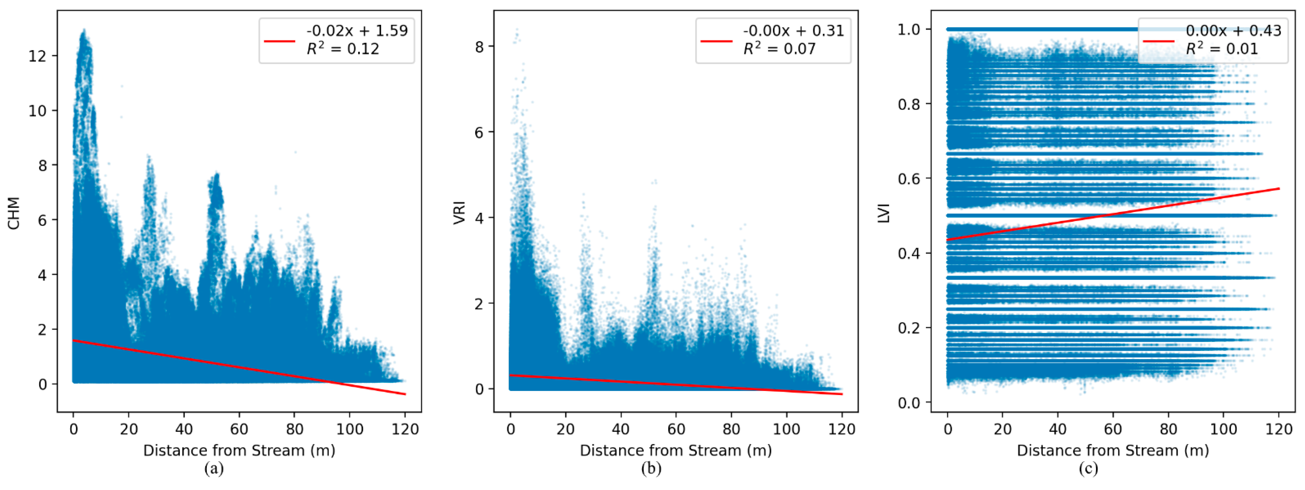
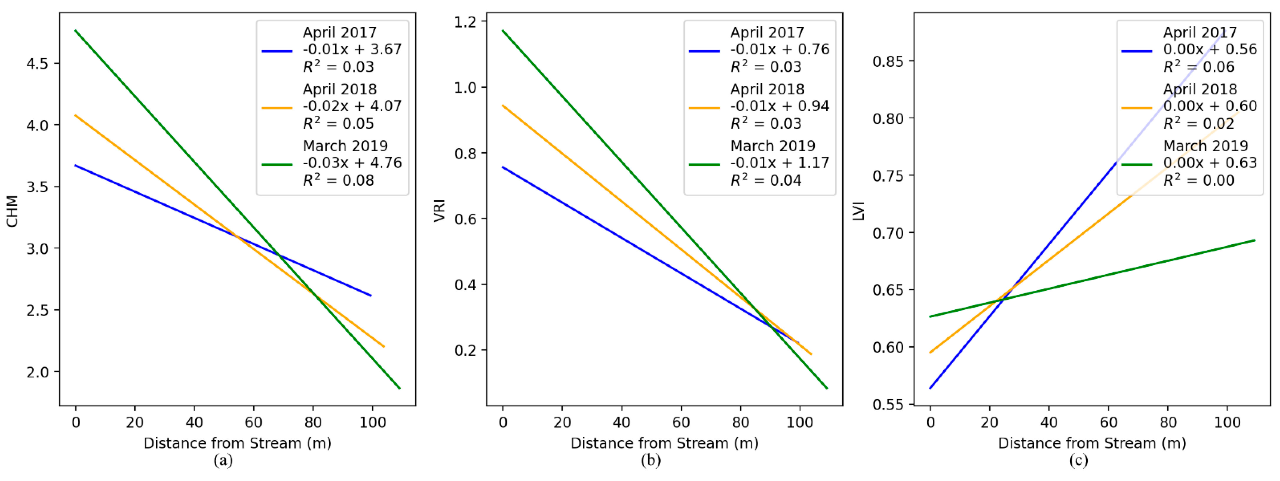
• Trees closer to the stream (within 20 m) grew faster than trees farther from the stream (greater than 20 m), although this trend was not observed with scrub.
• The trends observed in height (CHM) and roughness (VRI) were very similar and the differences were mainly in terms of the scale of each metric between scrub and trees.
• Height (CHM) and roughness (VRI) were more influenced by annual change.
• Density (LVI) was more influenced by seasonal variability.

Based on these results, it is clear that all three metrics are representing different aspects of the riverscape vegetation as it changes both annually and seasonally. It is recommended that for any fluvial application able to utilize high-resolution survey data such as from DLS, whether it is for ecological modeling or hydraulic modeling, to consider integrating all three metrics as possible explanatory variables to describe the dynamic physical changes occurring to vegetation over the riverscape.

References

1. Fausch, K.D.; Torgersen, C.E.; Baxter, C.V.; Li, H.W. Landscapes to Riverscapes: Bridging the Gap between Research and Conservation of Stream Fishes. BioScience 2002, 52, 483–498. [Google Scholar] [CrossRef] [Green Version]
2. Carbonneau, P.; Fonstad, M.A.; Marcus, W.A.; Dugdale, S.J. Making Riverscapes Real. Geomorphology 2012, 137, 74–86. [Google Scholar] [CrossRef]
3. Dietrich, J.T. Riverscape Mapping with Helicopter-Based Structure-from-Motion Photogrammetry. Geomorphology 2016, 252, 144–157. [Google Scholar] [CrossRef]
4. Farid, A.; Rautenkranz, D.; Goodrich, D.C.; Marsh, S.E.; Sorooshian, S. Riparian Vegetation Classification from Airborne Laser Scanning Data with an Emphasis on Cottonwood Trees. Can. J. Remote Sens. 2006, 32, 15–18. [Google Scholar] [CrossRef]
5. Heritage, G.; Hetherington, D. Towards a Protocol for Laser Scanning in Fluvial Geomorphology. Earth Surf. Process. Landf. 2007, 32, 66–74. [Google Scholar] [CrossRef]
6. Resop, J.P.; Kozarek, J.L.; Hession, W.C. Terrestrial Laser Scanning for Delineating In-Stream Boulders and Quantifying Habitat Complexity Measures. Photogramm. Eng. Remote Sens. 2012, 78, 363–371. [Google Scholar] [CrossRef] [Green Version]
7. Woodget, A.S.; Austrums, R.; Maddock, I.P.; Habit, E. Drones and Digital Photogrammetry: From Classifications to Continuums for Monitoring River Habitat and Hydromorphology. Wiley Interdiscip. Rev. Water 2017, 4, 1–20. [Google Scholar] [CrossRef] [Green Version]
8. Yang, B.; Hawthorne, T.L.; Torres, H.; Feinman, M. Using Object-Oriented Classification for Coastal Management in the East Central Coast of Florida: A Quantitative Comparison between UAV, Satellite, and Aerial Data. Drones 2019, 3, 60. [Google Scholar] [CrossRef] [Green Version]
9. Resop, J.P.; Lehmann, L.; Hession, W.C. Drone Laser Scanning for Modeling Riverscape Topography and Vegetation: Comparison with Traditional Aerial Lidar. Drones 2019, 3, 35. [Google Scholar] [CrossRef] [Green Version]
10. Huang, C.; Peng, Y.; Lang, M.; Yeo, I.-Y.; McCarty, G. Wetland Inundation Mapping and Change Monitoring Using Landsat and Airborne LiDAR Data. Remote Sens. Environ. 2014, 141, 231–242. [Google Scholar] [CrossRef]
11. Anders, N.S.; Seijmonsbergen, A.C.; Bouten, W. Geomorphological Change Detection Using Object-Based Feature Extraction from Multi-Temporal LiDAR Data. IEEE Geosci. Remote Sens. Lett. 2013, 10, 1587–1591. [Google Scholar] [CrossRef] [Green Version]
12. Okyay, U.; Telling, J.; Glennie, C.L.; Dietrich, W.E. Airborne Lidar Change Detection: An Overview of Earth Sciences Applications. Earth-Sci. Rev. 2019, 198, 102929. [Google Scholar] [CrossRef]
13. Resop, J.P.; Hession, W.C. Terrestrial Laser Scanning for Monitoring Streambank Retreat: Comparison with Traditional Surveying Techniques. J. Hydraul. Eng. 2010, 136, 794–798. [Google Scholar] [CrossRef]
14. O’Neal, M.A.; Pizzuto, J.E. The Rates and Spatial Patterns of Annual Riverbank Erosion Revealed through Terrestrial Laser-Scanner Surveys of the South River, Virginia. Earth Surf. Process. Landf. 2011, 36, 695–701. [Google Scholar] [CrossRef]
15. Saarinen, N.; Vastaranta, M.; Vaaja, M.; Lotsari, E.; Jaakkola, A.; Kukko, A.; Kaartinen, H.; Holopainen, M.; Hyyppä, H.; Alho, P. Area-Based Approach for Mapping and Monitoring Riverine Vegetation Using Mobile Laser Scanning. Remote Sens. 2013, 5, 5285–5303. [Google Scholar] [CrossRef] [Green Version]
16. Day, S.S.; Gran, K.B.; Belmont, P.; Wawrzyniec, T. Measuring Bluff Erosion Part 1: Terrestrial Laser Scanning Methods for Change Detection. Earth Surf. Process. Landf. 2013, 38, 1055–1067. [Google Scholar] [CrossRef]
17. Flener, C.; Vaaja, M.; Jaakkola, A.; Krooks, A.; Kaartinen, H.; Kukko, A.; Kasvi, E.; Hyyppä, H.; Hyyppä, J.; Alho, P. Seamless Mapping of River Channels at High Resolution Using Mobile LiDAR and UAV-Photography. Remote Sens. 2013, 5, 6382–6407. [Google Scholar] [CrossRef] [Green Version]
18. Leyland, J.; Hackney, C.R.; Darby, S.E.; Parsons, D.R.; Best, J.L.; Nicholas, A.P.; Aalto, R.; Lague, D. Extreme Flood-Driven Fluvial Bank Erosion and Sediment Loads: Direct Process Measurements Using Integrated Mobile Laser Scanning (MLS) and Hydro-Acoustic Techniques. Earth Surf. Process. Landf. 2017, 42, 334–346. [Google Scholar] [CrossRef]
19. Andersen, H.-E.; McGaughey, R.J.; Reutebuch, S.E. Estimating Forest Canopy Fuel Parameters Using LIDAR Data. Remote Sens. Environ. 2005, 94, 441–449. [Google Scholar] [CrossRef]
20. Huang, W.; Dolan, K.; Swatantran, A.; Johnson, K.; Tang, H.; O’Neil-Dunne, J.; Dubayah, R.; Hurtt, G. High-Resolution Mapping of Aboveground Biomass for Forest Carbon Monitoring System in the Tri-State Region of Maryland, Pennsylvania and Delaware, USA. Environ. Res. Lett. 2019, 14, 095002. [Google Scholar] [CrossRef] [Green Version]
21. Mundt, J.T.; Streutker, D.R.; Glenn, N.F. Mapping Sagebrush Distribution Using Fusion of Hyperspectral and Lidar Classifications. Photogramm. Eng. Remote Sens. 2006, 72, 47–54. [Google Scholar] [CrossRef] [Green Version]
22. Arcement, G.J.; Schneider, V.R. Guide for Selecting Manning’s Roughness Coefficients for Natural Channels and Flood Plains; United States Geological Survey: Denver, CO, USA, 1989.
23. You, H.; Wang, T.; Skidmore, A.K.; Xing, Y. Quantifying the Effects of Normalisation of Airborne LiDAR Intensity on Coniferous Forest Leaf Area Index Estimations. Remote Sens. 2017, 9, 163. [Google Scholar] [CrossRef] [Green Version]
24. Kato, A.; Moskal, L.M.; Schiess, P.; Swanson, M.E.; Calhoun, D.; Stuetzle, W. Capturing Tree Crown Formation through Implicit Surface Reconstruction Using Airborne Lidar Data. Remote Sens. Environ. 2009, 113, 1148–1162. [Google Scholar] [CrossRef]
25. Jakubowski, M.K.; Li, W.; Guo, Q.; Kelly, M. Delineating Individual Trees from Lidar Data: A Comparison of Vector- and Raster-Based Segmentation Approaches. Remote Sens. 2013, 5, 4163–4186. [Google Scholar] [CrossRef] [Green Version]
26. Wu, X.; Shen, X.; Cao, L.; Wang, G.; Cao, F. Assessment of Individual Tree Detection and Canopy Cover Estimation Using Unmanned Aerial Vehicle Based Light Detection and Ranging (UAV-LiDAR) Data in Planted Forests. Remote Sens. 2019, 11, 908. [Google Scholar] [CrossRef] [Green Version]
27. Dorn, H.; Vetter, M.; Höfle, B. GIS-Based Roughness Derivation for Flood Simulations: A Comparison of Orthophotos, LiDAR and Crowdsourced Geodata. Remote Sens. 2014, 6, 1739–1759. [Google Scholar] [CrossRef] [Green Version]
28. Lefsky, M.A.; Harding, D.J.; Keller, M.; Cohen, W.B.; Carabajal, C.C.; Espirito-Santo, F.D.B.; Hunter, M.O.; de Oliveira, R. Estimates of Forest Canopy Height and Aboveground Biomass Using ICESat. Geophys. Res. Lett. 2005, 32. [Google Scholar] [CrossRef] [Green Version]
29. Zhou, T.; Popescu, S. Waveformlidar: An R Package for Waveform LiDAR Processing and Analysis. Remote Sens. 2019, 11, 2552. [Google Scholar] [CrossRef] [Green Version]
30. Chow, V.T. Open-Channel Hydraulics; McGraw-Hill: New York, NY, USA, 1959; ISBN 978-0-07-085906-7. [Google Scholar]
31. Prior, E.M.; Aquilina, C.A.; Czuba, J.A.; Pingel, T.J.; Hession, W.C. Estimating Floodplain Vegetative Roughness Using Drone-Based Laser Scanning and Structure from Motion Photogrammetry. Remote Sens. 2021, 13, 2616. [Google Scholar] [CrossRef]
32. Barilotti, A.; Sepic, F.; Abramo, E.; Crosilla, F. Improving the Morphological Analysis for Tree Extraction: A Dynamic Approach to Lidar Data. In Proceedings of the ISPRS Workshop on Laser Scanning 2007 and SilviLaser 2007, Espoo, Finland, 12–14 September 2007. [Google Scholar]
33. Wynn, T.; Hession, W.C.; Yagow, G. Stroubles Creek Stream Restoration; Virginia Department of Conservation and Recreation: Richmond, VA, USA, 2010.
34. Wynn-Thompson, T.; Hession, W.C.; Scott, D. StREAM Lab at Virginia Tech. Resour. Mag. 2012, 19, 8–9. [Google Scholar] [CrossRef]
35. YellowScan YellowScan Surveyor: The Lightest and Most Versatile UAV LiDAR Solution. Available online: https://www.yellowscan-lidar.com/products/surveyor/ (accessed on 21 March 2020).
36. Isenburg, M. Processing Drone LiDAR from YellowScan’s Surveyor, a Velodyne Puck Based System. Available online: https://rapidlasso.com/2017/10/29/processing-drone-lidar-from-yellowscans-surveyor-a-velodyne-puck-based-system/ (accessed on 4 September 2021).
37. Wheaton, J.M.; Brasington, J.; Darby, S.E.; Sear, D.A. Accounting for uncertainty in DEMs from repeat topographic surveys: Improved sediment budgets. Earth Surf. Process. Landf. 2010, 35, 136–156. [Google Scholar] [CrossRef]
38. Williams, R. DEMs of Difference. Geomorphol. Tech. 2012, 2, 1–17. [Google Scholar]
Figure 1. The study area, a 0.65 km reach of Stroubles Creek, showing the approximate extent of the drone laser scanning (DLS) surveys. The actual extent varied slightly between scans.
Drones 05 00091 g001
Figure 2. Photos of the study area, Stroubles Creek, taken downstream of the concrete bridge from an on-site tower camera around the same dates as the drone scans: (a) April 2017, (b) August 2017, (c) January 2018 (Note: Due to a malfunction in the tower camera, this is the closest photo to the November 2017 scan), (d) April 2018, (e) October 2018, (f) March 2019.
Drones 05 00091 g002
Figure 3. An example misaligned point cloud representing one of the wooden sampling bridges that cross the stream showing an elevation bias in the November 2017 scan (i.e., the green points) relative to the other scans before correction with CloudCompare.
Drones 05 00091 g003
Figure 4. The extent of each drone laser scanning (DLS) survey as well as the extent intersection of all six scans (“Seasonal Extent”) and of only the annual leaf-off season scans (April 2017, April 2018, and March 2019; “Annual Extent”).
Drones 05 00091 g004
Figure 5. The workflow deriving the canopy height model (CHM) based on the maximum height above ground of lidar vegetation points in each raster pixel.
Drones 05 00091 g005
Figure 6. The workflow estimating the vegetative roughness index (VRI) based on the standard deviation of vegetation height within each raster pixel.
Drones 05 00091 g006
Figure 7. The workflow calculating the lidar vegetation index (LVI) based on the percentage of vegetation points within each raster pixel as a measure of density.
Drones 05 00091 g007
Figure 8. Drone laser scanning (DLS) point classifications within the extent intersection over all six scans showing the seasonal variation between terrain points and vegetation points.
Drones 05 00091 g008
Figure 9. Trees taller than 2 m were identified from the April 2017 canopy height model (CHM) and maximum tree height was measured for: (a) April 2017; (b) April 2018; (c) March 2019.
Drones 05 00091 g009
Figure 10. Maximum tree height statistics of the 604 trees identified in the riverscape for each of the three leaf-off scans. The average and standard deviation of maximum tree height increased over the two-year period.
Drones 05 00091 g010
Figure 11. Lidar vegetation metrics for April 2017 showing: (a) height (CHM); (b) roughness (VRI); (c) density (LVI).
Drones 05 00091 g011
Figure 12. The relationship between vegetation metrics and distance to stream for April 2017: (a) height (CHM); (b) roughness (VRI); (c) density (LVI).
Drones 05 00091 g012
Figure 13. Trends in annual vegetation change over the riverscape: (a) total land class area; (b) average height (CHM); (c) average roughness (VRI); (d) average density (LVI).
Drones 05 00091 g013
Figure 14. Change matrices representing the pixel-level change in land class between: (a) April 2017 and April 2018; (b) April 2018 and March 2019.
Drones 05 00091 g014
Figure 15. DEMs of Difference (DoDs) over the two-year study from April 2017 to March 2019 representing pixel-level change in: (a) height (CHM); (b) roughness (VRI); (c) density (LVI).
Drones 05 00091 g015
Figure 16. The average pixel-level annual change in each metric, (a) height (CHM), (b) roughness (VRI), and (c) density (LVI), over each land class and over each year in the two-year study.
Drones 05 00091 g016
Figure 17. Linear regression models relating vegetation metrics and distance to stream annually over time for tree areas: (a) height (CHM); (b) roughness (VRI); (c) density (LVI).
Drones 05 00091 g017
Figure 18. Trends in seasonal vegetation change over the riverscape: (a) total land class area; (b) average height (CHM); (c) average roughness (VRI); (d) average density (LVI).
Drones 05 00091 g018
Figure 19. Trends in seasonal vegetation decay over the riverscape going from August (2017) to October (2018) to November (2017) to April (2018): (a) total land class area; (b) average height (CHM); (c) average roughness (VRI); (d) average density (LVI).
Drones 05 00091 g019