Article

Modeling and Investigations on Surface Colors of Wings on the Performance of Albatross-Inspired Mars Drones and Thermoelectric Generation Capabilities

1
Department of Mechanical and Aerospace Engineering, New Mexico State University, Las Cruces, NM 88003, USA
2
Department of Engineering Technology and Surveying Engineering, New Mexico State University, Las Cruces, NM 88003, USA
3
Los Alamos National Laboratory, Los Alamos, NM 87545, USA
*
Author to whom correspondence should be addressed.
Drones 2020, 4(3), 43; https://doi.org/10.3390/drones4030043
Submission received: 28 July 2020 / Revised: 12 August 2020 / Accepted: 13 August 2020 / Published: 16 August 2020
(This article belongs to the Special Issue Feature Papers of Drones)

Abstract

:
Thermal effects of wing color for Albatross-inspired drones performing in the Martian atmosphere are investigated during the summer and winter seasons. This study focuses on two useful consequences of the thermal effects of wing color: the drag reduction and the thermoelectric generation of power. According to its color, each wing side has a certain temperature affecting the drag. Investigations of various configurations have shown that the thermal effect on the wing boundary layer skin drag is insignificant because of the low atmospheric pressure. However, the total drag varies as much as 12.8% between the highest performing wing color configuration and the lowest performing configuration. Additionally, the large temperature differences between the top and the bottom wing surfaces show great potential for thermoelectric power generation. The maximum temperature differences between the top and bottom surfaces for the summer and winter seasons are, respectively, 65 K and 30 K. The drag reduction and the power generation via thermoelectric generators both contribute to enhancing the endurance of drones. Future drone designs will benefit from increased endurance through optimizing the wing color configuration.

1. Introduction

Over the past few decades, various government and private programs have been developed for space exploration. Among the high interest exploration targets is the planet Mars. NASA has performed many missions in the past and will continue with new mission in the future including the upcoming Mars 2020 mission [1]. The private company, SpaceX, hopes to establish a supply depot on Mars by the year 2024 as a cornerstone for future manned missions to the planet [2]. As Mars begins to generate greater interest in the near future, planetary exploration will become much more important. The current methods used to explore the Martian surface include rover, lander, and satellite [3]. In the past few years, the concept of using drones for planetary exploration has gained traction and many design concepts have been developed [3]. To design a drone suitable for Mars exploration, it is important to understand the Martian atmosphere and other properties for flight. Compared to Earth, the atmosphere of Mars is much thinner, and the temperature is also colder [4]. Atmospheric properties such as density, pressure, and temperature were obtained at varying altitudes from the high-speed entry of a probe into the atmosphere [5].
Due to the extreme conditions and challenges associated with flying in the Martian atmosphere, maximizing the efficiency of a drone is essential [3,4]. Drones require high endurance to be able to perform many defined missions for planetary exploration. The endurance of a drone is primarily limited by the available energy [6]. There are various propulsion systems and fuel/oxidizers that provide energy for drones, and there are additional methods, such as solar cells, batteries, etc., that provide energy to the drone [7,8]. Solar cells have been gaining popularity for use in space exploration for several systems. Orbitals and drones have had studies performed for Solar Electric Propulsion (SEP) applications [9,10]. When considering enhancing the endurance of a drone, there are various methods to take into consideration. Optimizing the propulsion system to increase the total available energy is one option. In the case of an electric propulsion system, recharging the battery by various means can enhance the endurance of the drone. Solar panel methods have been researched as a possible option to power or partially power drones [11,12,13,14]. Additionally, thermoelectric generators are another possible method to harness energy via converting the thermal energy from the temperature difference between two surfaces to electrical power [15]. Another option for enhancing the endurance of a drone is to optimize the structure so that energy can be best conserved which will result in a reduction of necessary power [16,17,18,19,20,21]. Control algorithms have also a great impact on the energy consumption [22,23].
Researchers have explored various techniques to decrease and manage the required power for drones. An example is to propose new design methods for drones, which improve their aerodynamic and mechanical efficiencies and consequently reduce the power consumption. Therefore, design methods enhance the performance and efficiency of drones which will extend their endurance and improve their utility in complex environments. Reduction of drag can be considered one of the main factors during the design process to conserve energy for the mission. In other words, drag reduction of fixed wing drones is crucial to flight efficiency on Mars [24].
The structure of a fixed wing drone can come in many different shapes and sizes. Often, when trying to optimize a drone, inspiration can be sought from nature. As seen from nature, on Earth there exists different modes of flight depending on the species of bird including flapping, hovering, gliding, and soaring [25]. Specifically, soaring and gliding are flight modes that are used by fixed wing drones. The nature of a bird’s mode of flight was used in a study to design a drone capable of wing morphing. Two different flight conditions were achieved through either sweeping or spanning the wing [26]. Another study was previously performed to analyze the thermal effects of wing color on the resulting heated boundary layer flow over the wing of an Albatross [27]. The study analyzed different wing color configurations to identify the most efficient configuration. The results verify the drag efficiency of the natural wing color configuration of the Albatross (which is black on the top surface and white on the bottom surface) compared to other color configurations. To design an efficient drone capable of flying in the Martian atmosphere, a similar study will be performed to analyze the thermal effects of wing color on the heated boundary layer of an Albatross wing shape within the Martian atmosphere. To the authors’ knowledge, a thermal boundary layer analysis of wing color configurations for drag efficiency calculations of a drone based on wing color on Mars has not been previously performed. This study will provide information on the surface temperature of a wing during different seasons and for different color configurations. An optimal wing color configuration will be determined to achieve maximum drag efficiency. Additionally, due to a possible temperature difference between the top and bottom wing surfaces, an investigation into the application of thermoelectric generators (TEGs) will be performed. Thermoelectric generators are composed of semiconductor material that produces thermoelectric modules. These modules are between ceramic wafers and then connected to an electrical load resistance. Electrical power is generated from the temperature difference as a result that can be explained through the Seebeck effect. The specific type of TEG considered for this study is the BiTe which is considered suitable for low-temperature heat recovery applications [28,29,30].
The paper is organized as follows: the thermal model describing the energy balance, wing color configurations, and the surrounding temperatures and heat fluxes is discussed in Section 2. Section 3 considers both the wing surfaces to investigate the skin drag forces and the effects of the angle of attack. A 3D aerodynamic analysis is performed to determine the total drag forces in Section 4. Section 5 studies the application of thermoelectric generators for drones in the Martian atmosphere. A summary and conclusions are drawn in Section 6.

2. Mathematical Model

An analytical model is developed using an energy balance to determine the wing surface temperature and consequently the skin friction drag. Atmospheric properties, such as sky, ground, and ambient temperatures are determined and applied to the energy balance. Each section of the energy balance is discussed in detail for the following sections: solar energy absorption, convective heat transfer, and radiative heat transfer. The conductive heat transfer will be defined in Section 4.

2.1. Energy Balance

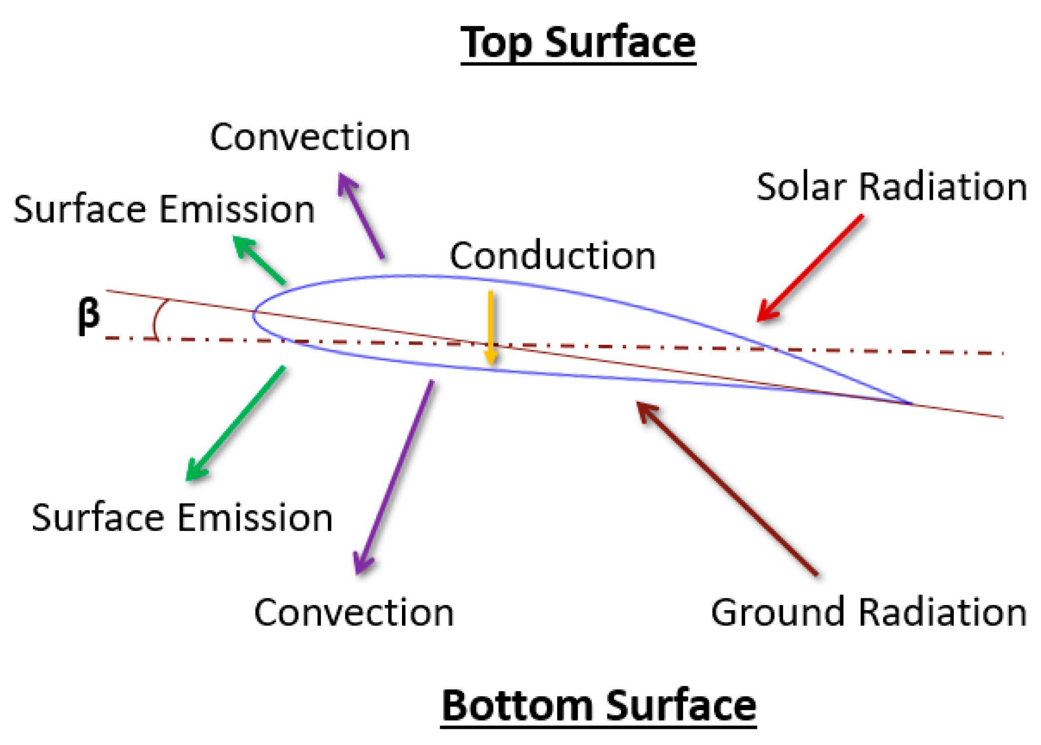
To understand the thermal effects of different wing colors, a thermal analysis is performed using an energy balance and including the influences of solar energy absorption, convection heat loss, and radiative heat loss. The energy balance on a drone fixed wing can be expressed as:
P solar = P convective + P radiative + P conductive
The various sources of energy acting on the wing can be seen in Figure 1. The absorbed solar radiation is balanced by the convective, radiative and conductive transfer. Determining the various fluxes in the energy balance requires information from the Martian atmosphere. In this study, the ambient temperature, pressure, wind speed, and other atmospheric properties are obtained from the dataset collected by Viking Lander 1 and the entry probe (VL1), which is located at 22.37 N latitude and 47.97 W longitude on the surface of Mars [31].
The top and the bottom wing surfaces experience different heat fluxes, which can be determined by the view factors, surface temperatures, surface absorptance, and surface emissivity. The total energy balance equations for both the top and the bottom surfaces of the wing are given in Equations (2) and (3), respectively [32].
α t · G b · cos θ + α t · F d t · G dh + α t · al · F al t · ( G bh + G dh ) h · ( T s top T amb ) ε t · σ · F d t · ( T s - top 4 T sky 4 ) ε t · σ · F al t · ( T s top 4 T grd 4 ) 1 R eff · ( T s - top T s - bottom ) = 0
α b · F d b · G dh + α b · al · F al b · ( G bh + G dh ) h · ( T s - bottom T amb ) ε b · σ · F d b · ( T s - bottom 4 T sky 4 ) ε b · σ · F al b · ( T s - bottom 4 T grd 4 ) 1 R eff · ( T s - bottom T s - top ) = 0
In the energy balance equations, the meanings of the different symbols are detailed in the nomenclature, using subscripts t and b to denote top and bottom wing surface, respectively. The convective heat transfer coefficient, denoted h is obtained from calculating the Nusselt Number on a flat plate in laminar regime as detailed in [33] using Mars atmospheric properties and assuming that the dominant gas is C O 2 . These properties were obtained from [34]. The atmospheric density was determined by using ideal gas law at 8.5 mbar of atmospheric pressure.

2.2. Sky, Ground, and Ambient Temperatures

As mentioned previously, this study includes the summer and winter seasons. As such, the sky, ground, and ambient temperatures for both seasons are needed. The information for a summer day corresponds to a solar longitude of 140 ° and for a winter day corresponds to a solar longitude of 280 ° . Figure 2 shows the ambient temperatures based on the season. The ambient temperature for summer is higher than winter and has a larger variation over the day. The summer daily variation has a range of almost 50 °C, while the winter only has a daily variation of nearly 15 °C [31]. Figure 3 shows the sky and ground temperatures as reported by Matz et al. [32] at the same location on the same day. The ground temperature follows a similar trend where the summer temperatures are higher and vary more throughout the day compared to the winter ground temperatures. The sky temperatures, however, have the opposite trend. The winter sky temperature is higher and varies more compared to the summer sky temperatures.

2.3. Solar Energy Absorption

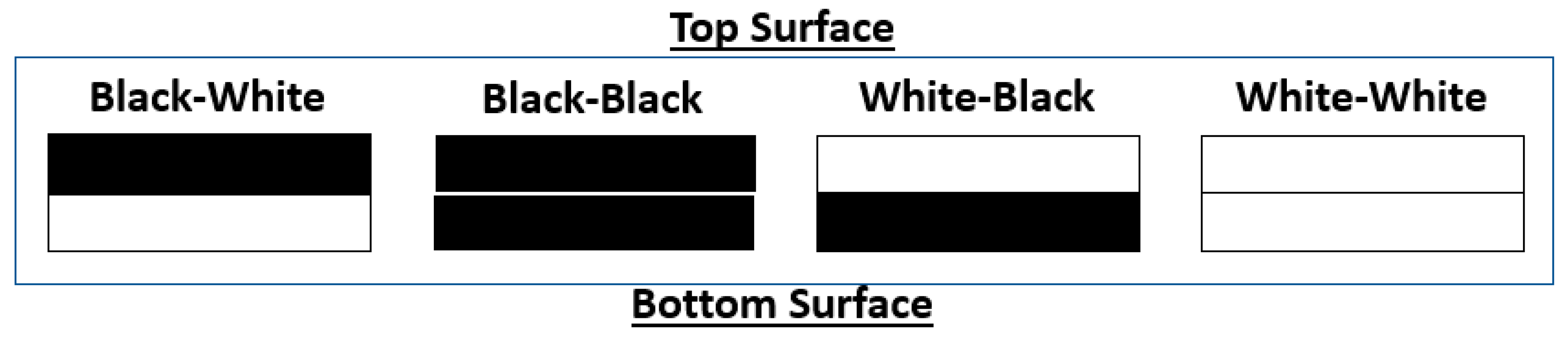
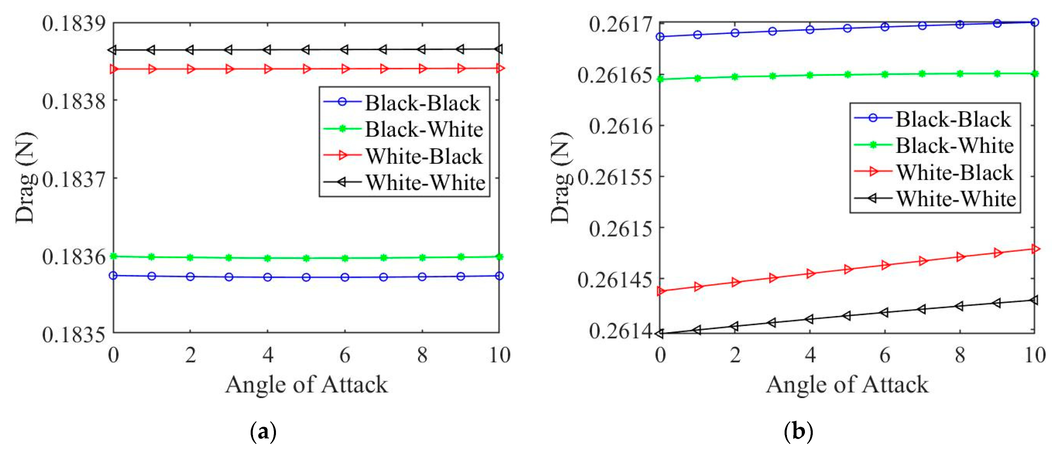
Being inspired by migrating birds’ flight on Earth, different color combinations are investigated. It is assumed that the top and bottom surfaces have different colors and therefore different absorptivity values. The different color configurations considered during this study are shown in Figure 4. The four configurations are on the top and bottom surfaces, respectively, black–white, black–black, white–black, and white–white. The solar irradiance that acts on the top surface of the wings includes direct beam, diffuse, and albedo radiations. The wing surface exposure to different radiation fluxes is governed by the view factors to the sky and the ground. The absorbed energy on the two wing surfaces can be written as [32]:
P solar - top = α t · G b · cos θ + α t · F d t · G dh + α t · al · F al t · ( G bh + G dh )
P solar - bottom = α b · F d b · G dh + α b · al · F al b · ( G bh + G dh )
The view factors for the top and bottom surfaces are needed and are expressed by Equations (6)–(9), where β is the angle of attack. The view factor for the top surface to the sky is F d t while the view factor for the top surface to the ground is F a l t . For the bottom surface, the view factor for the bottom to the sky F d b is identical to F a l t . Likewise, the view factor from the bottom surface to the ground F a l b is identical to F d t . In this case, the drone is considered to be flying very close to the ground because some of the atmospheric properties used were measured by VL1 at ground level. It is noted that at a zero-degree angle of attack Equations (2) and (3) are decoupled because the view factor from the top surface to the sky is 1 and the view factor for the top surface to the ground is zero.
F d t = 1 + cos β 2
F a l t = 1 cos β 2
F d b = F a l t
F a l b = F d t
The absorptivity values for α t and α b used in this study are 0.88 and 0.23, which correspond to the absorptance of anodize black paint and biphenyl white solid paint, respectively. Both are often used for space applications [35]. Depending on several variables, such as the solar angle of incidence shown in Figure 5, the optical depth of the Martian atmosphere, and the season, the solar irradiance changes. NASA researchers from Lewis Research Center in Ohio have derived a set of equations to determine the solar irradiance on Mars [36]. One of the most crucial elements for determining the solar irradiance is the position of the wing with respect to the sun. The solar incidence angle θ is used to describe this relation and can be determined from Equation (10), as follows [37]:
cos θ = sin φ sin δ cos β sin δ cos φ cos λ sin β + cos φ cos δ cos ω cos β + cos δ sin φ cos λ cos ω sin β + cos δ sin λ sin ω sin β
To determine the solar incidence angle, positional information about the drone must be known, such as the latitude φ , declination angle δ , hour angle ω , angle of attack β , and the wing azimuth angle λ . The wing azimuth angle can be considered as the direction of flight. In this study, the drone is assumed to be flying directly southward. The hour angle only considers daylight hours from 7:00 to 17:00. Additionally, the hour angle refers to solar Martian time (0:00–24:00). The declination angle depends on the season which is described by the areocentric longitude L s . The latitude selected for the study is the location of the rover which is where the atmospheric properties are obtained. The values for latitude, declination angle, tilt angle, and wing azimuth angle that are used in this study are shown in Table 1 for both summer and winter seasons.
After determining the solar incidence angle, the solar irradiance can then be determined. The direct beam irradiance G b , diffuse irradiance on a horizontal surface G d h , and the global irradiance on a horizontal surface G h which are used to determine the beam, diffuse, and albedo irradiance, respectively, can be determined from Equations (11)–(13) [36]. The optical depth τ varies depending on the date which is represented by the areocentric longitude L s . The optical depth is a result of the atmospheric dust particles in the atmosphere [38]. The values for the solar irradiance variables that are used for this study are shown in Table 2. The normalized net flux function f ( θ , τ ) values [36] used during this study that correspond to the solar incidence angle and optical depth are presented in Table 3.
G b = G ob · e ( τ cos θ )
G d h = G h G b h
G h = G ob · cos θ · f ( θ , τ ) 1 al
The solar irradiance at the top of the atmosphere G ob , which can be seen in Equation (14) [36], is needed along with the optical depth τ , solar incidence angle θ , and the normalized net flux function f ( θ , τ ) to determine the direct beam irradiance and the global irradiance. Mars eccentricity b is around 0.093377, as can be seen in Table 2. The diffuse irradiance can be determined by subtracting the direct beam irradiance on a horizontal surface G b h from the global irradiance on a horizontal surface G h . The equation for direct beam irradiance on a horizontal surface can be expressed as shown in Equation (15) [36].
G ob = 590 · [ 1 + b · cos ( L s 248 ° ) ] 2 ( 1 b 2 ) 2
G bh = G ob · cos θ · e ( τ cos θ )

2.4. Radiative Heat Loss

Equations (16) and (17) represent the radiative heat loss for the top and bottom wing surfaces, respectively. The top and bottom wing surfaces will differ depending on the emissivity ε and the shape factors. For a zero-degree angle of attack, the top wing surface only loses energy to the sky while the bottom wing surface only loses energy to the ground. The values used for emissivity are based on anodize black paint and biphenyl white solid paint, respectively. For both white and black colors, the emissivity is 0.88 [24]. The sky and ground temperatures can be found in Figure 3a,b, respectively.
P radiative - top = ε t · σ · F dt · ( T s - top 4 T sky 4 ) + ε t · σ · F alt · ( T s - top 4 T grd 4 )
P radiative - bottom = ε b · σ · F db · ( T s - bottom 4 T sky 4 ) + ε b · σ · F alb · ( T s - bottom 4 T grd 4 )

2.5. Thermal Boundary Layer Analysis

For simplicity, the wing curvature is ignored, and a flat plate is considered for the boundary layer analysis. Figure 6 represents a schematic view of the boundary layer over a flat plat [25].
The thermal boundary layer effects on the skin friction drag are determined using Equation (18) [39], where the wingspan ws , is 3.5 m and the chord length, L , is 0.22 m [7]. To determine the viscosity μ , Sutherland’s formula, which can be found in Equation (19), is used [40]. T 0   and   μ 0 are the reference temperature and viscosity, respectively, which are 293.14 K and 1.48 × 10 5 kg m · s for the Martian atmosphere [41]. The Sutherland constant C, for CO 2 is 240 K [41] and T s 
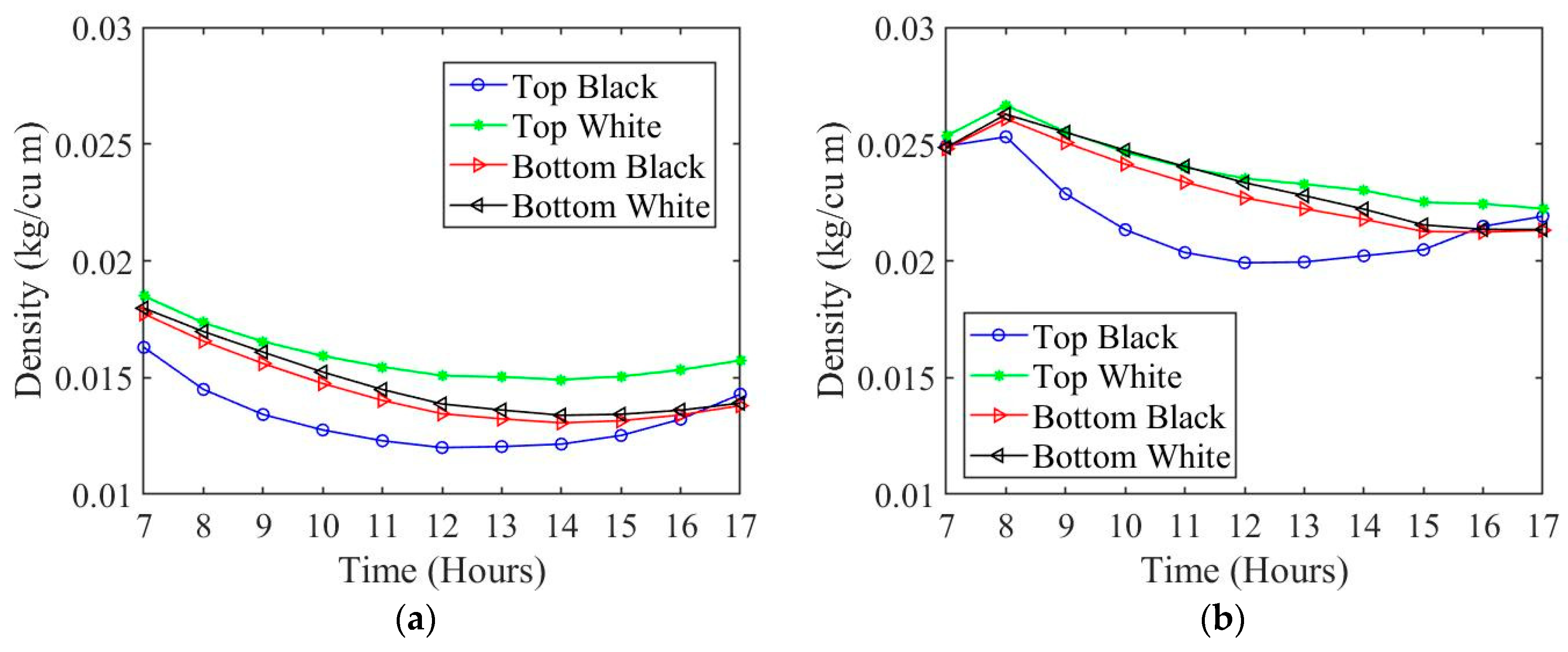
is the wing surface temperature. The density ρ is determined using ideal gas law considering CO 2 in Equation (20). The ideal gas constant for the Martian atmosphere R , is 192.1   J kg · K [30]. The pressure P is found from the information collected by VL1.
D = 0.664 · ws · ρ · μ · u 3 · L
μ = μ 0 · ( T 0 + C T s + C ) · ( T s T 0 ) 3 / 2
ρ = P 192.1 R · T s

3. Wing Surface Analysis

In this section, the whole wing (top and bottom surfaces) is considered for the study. The wing structure will be considered as a hollow wing composed of a hollow center with a top layer and a bottom layer of material. The model of the overall wing can be seen in Figure 7a,b. From Figure 7b, it can be observed that the conductive heat transfer will cover three layers of material; the first layer of material, the interior which is air (CO2 for the Martian atmosphere), and the third layer of material.
The expression for heat conduction is given in Equation (21), where the conduction is determined from the temperature difference between the top surface Ts-top, and the bottom surface Ts-bottom divided by the effective resistance of all materials. The effective resistance is presented in Equation (22) where Lsurface is the depth of the wing material, Lair is the average depth of the hollow part of the wing, Ksurface denotes the thermal conductivity of the material, Kair represents the thermal conductivity of the Martian atmosphere, Asurface is the area of the material, and Aair denotes the area of the hollow part.
P conductive = T s - top T s - bottom R eff
R eff = 2 L s u r f a c e K surface A surface + L air K air A air
Air (CO2) acts as an insulator in this case which prevents conductive heat transfer from occurring between the top surface and the bottom surface. The surface temperature for the top and bottom surfaces with and without considering conductive heat fluxes are shown in Figure 8 for summer.
Air has a very low thermal conductivity, which will result in a very high thermal resistance. The heat conducted through the wing can be considered negligible compared to the total energy balance. This allows Equations (2) and (3) to be simplified into Equations (23) and (24). The two new energy balance equations become uncoupled without the conductive heat transfer and are used for the rest of this study.
α t · G b · cos z + α t · F d t · G dh + α t · al · F al t · ( G bh + G dh ) h · ( T s - top T amb ) ε t · σ · F d t · ( T s - top 4 T sky 4 ) ε t · σ · F al t · ( T s - top 4 T grd 4 ) = 0
α b · F d b · G dh + α b · al · F al b · ( G bh + G dh ) h · ( T s - bottom T amb ) ε b · σ · F d b · ( T s - bottom 4 T sky 4 ) ε b · σ · F al b · ( T s - bottom 4 T grd 4 ) = 0
When considering an angle of attack of zero degrees, the equations are completely decoupled and thus can be solved individually. Therefore, the effects of the conduction are not considered in further analysis. As can be seen in Figure 9a,b, the solar absorption for the top surface (both white and black colors) are higher than the bottom surface. This is due to the direct beam irradiance that is only experienced by the top surface. Additionally, the solar absorption during summer is higher than during the winter due to the high solar intensity that occurs during the summer period of the Martian solar cycle.
The two new energy balance Equations (23) and (24) can then be used to determine the surface temperature for both the bottom and top wing surfaces for black and white wing colors as presented in Figure 10. During the summer and winter seasons, the wing surface experiences the highest temperatures when a black color is applied to the top surface. The lowest wing temperatures occur when white paint is used on the top surface. As expected, due to the high solar absorption during summer, the overall temperatures on the wing surfaces are higher during summer compared to winter.
Using the surface temperature, Equations (18)–(22) can be solved to find the viscosity, density, and drag. The viscosity for both wing surfaces and for black and white colors are plotted in Figure 11a,b, respectively. The viscosity follows a similar trend to the surface temperature. The higher surface temperature wing color configuration results in a higher viscosity along the boundary. The density, which can be seen in Figure 12a, is lower along the boundary layer when the surface temperature is higher. The total drag of the combined wing color configurations is plotted in Figure 13a,b for summer and winter, respectively. The four different wing color combinations are as follows: black on top and black on bottom (black–black), black on top and white on bottom (black–white), white on top and black on bottom (white–black), and white on top and white on bottom (white–white). It follows from Figure 13a, during the summer, that the highest drag color configuration is the white–white, and the lowest drag is the black–black. During the winter, it is shown in Figure 13b that the highest drag is from the color configuration black–black and the lowest drag is from the color configuration white–white.
Comparing the relative change between the highest drag color configuration and the lowest drag color configuration results in Figure 13a,b. During the summer the highest drag color configuration is white–white and the lowest is the black–black color configuration. During the winter, the trend is reversed with the highest drag color configuration being black–black and the lowest color configuration white–white.
During the summer season, the optimal wing color configuration is black–black which results in a decrease of drag by a maximum of 0.125% compared to the white–white wing color configuration. During the winter season, the optimal wing color configuration is white–white which has a maximum drag reduction of 0.15% compared to the black–black configuration, as shown in Figure 14.
Until now, the results have been generated using a zero-degree angle of attack (AoA). To understand the effects of the angle of attack, the drag as a function of angle of attack at solar noon is plotted in Figure 15. The change in drag during the summer period is near constant over a range of 10 degrees AoA. During the winter, the maximum change in drag occurs for the white–black color configuration with a change percentage of 0.001%. It can be concluded that the change in angle of attack is negligible to determining the drag force. This led to using a constant zero-degree angle of attack for the study.

4. 3D Aerodynamic Analysis

The skin friction drag has already been determined based on the boundary layer analysis in Section 3. In this section, the aerodynamic performance for the whole wing will be analyzed by determining the total drag. The drag will be determined using an aerodynamic analysis software named XFLR5. The total drag includes the form drag, the induced drag, and the parasitic drag. The software used to analyze the 3D wing geometry can determine the drag coefficients. The study considers a constant zero-degree angle of attack under similar conditions as the boundary layer analysis from Section 3 and the two results are compared. Four analysis methods, namely, Lifting Line Theory (LLT), Horseshoe Vortex (VLM1), Ring Vortex (VLM2), and 3D panel method are used in order to estimate the total drag of an Albatross-inspired drone in the Martian atmosphere. All of these methods consider the assumption of inviscid flow.
The LLT method uses the assumption that the lift coefficient as a function of the angle of attack is linear. One major assumption for the LLT method is that the surfaces are in the X-Y plane and that the dihedral angles and the sweep are not needed for the lift distribution calculations. The lift of the wing for this theory is determined from the incremental vortices shed along the trail span of the wing along the freestream direction [42].
The VLM1 and VLM2 methods allow for more freedom in the choice of wing geometry. This includes winglets, high dihedral angles, low aspect ratio, and sweep. For the VLM methods, the general idea is to model the perturbation of the wing planform using a vortices’ distribution sum. The lift coefficient is computed by integrated surface forces, such as the moment coefficients. The VLM methods calculate the lift distribution, induced angles, and induced drag. Because of this, the methods are independent of the wing speed. The VLM methods assume small angles of attack, so stall angles should be avoided when computing results. The main difference between the VLM1 and VLM2 methods is that the VLM1 method does not consider side slip [42].
The 3D panel method is able to account for the thickness of the wing unlike the VLM methods that only consider the mean camber line. Because of this, the 3D panel method can allow for an understanding of the center of pressure distribution over the top and bottom surfaces of the wing. The 3D panel method uses an approach that sum the doublets and sources distributed of the surface of the wing from the perturbations generated. The 3D panel method can be used to polish the results of the other three methods, so this is often considered to be the most accurate method. The 3D panel method will be considered as the standard for this study that the other three methods will be compared to [42].
As mentioned in the previous section, the 3D aerodynamic analysis methods all have inviscid assumptions. To account for the viscosity in the 3D analysis, a 2D viscous analysis is performed for the selected airfoil to obtain 2D viscous information. The 2D information is then interpolated and then incorporated into the 3D analysis and this is how the viscous effects are included in the analysis. The 2D boundary layer problem is solved using a software called XFoil by using an iterative method along with the inviscid velocity field as an input. The method provides a viscous velocity from the boundary layer solution which is used as an input for the potential flow solver. This iterative method is called the “Interactive Boundary Layer” [42]. The wing shape considered for the 3D analysis is that of an Albatross. Figure 16 shows the analyzed wing shape and Table 4 lists the geometric properties.
To solve the 2D and 3D analyses, certain properties are needed, namely, the Reynolds number and wing velocity. The wing velocity and the Reynolds number for the 3D analysis are the same as for the boundary layer analysis. The Reynolds number is calculated based on the viscosity and density found in Section 3. The total drag varies depending on the analysis method. As mentioned previously, the 3D panel method is considered to be the most accurate method and the other three methods are compared to the 3D panel method to determine their accuracy. The number of panels on the wing is determined in order for the different methods of analysis to converge. Figure 17 compares the total drag for the different analysis methods for both summer and winter. Inspecting the plotted curves in these figures, it is clear that VLM1 and VLM2 methods have comparable results to the 3D panel method. The LLT method varies greatly compared to the other three methods. In Table 5 and Table 6, the percent difference between the different methods compared to 3D panel method is shown. The percent difference between VLM1 and VLM2 compared to the 3D panel method is 3~4%, which shows good agreement. However, the LLT method compared to the 3D panel method has a greater than 50% error, which shows that the LLT method is not capable of handling the complex geometry of the Albatross-like wing shape.
The total drag forces for the wing at a constant angle of attack and at different times throughout the day is calculated using the 3D panel method. The total drag includes the form drag, the induced drag, and the parasitic drag. Figure 18 shows the total drag dependent on the hour for the 3D panel method. Compared to the drag determined using the boundary layer analysis, the drag calculated using the 3D panel method is much larger, by a factor of 5 on average. During the winter, the drag is much higher than during the summer. This remains consistent with the trend found for the skin friction drag. Additionally, the black–black wing color configuration is the most optimal case that results in the least amount of drag for both summer and winter. The percent change between the most optimal wing color configuration (black–black) and the least optimal color configuration (white–white) is much more significant when considering the total drag instead of just the skin drag. For summer the percent change is 12.6% and for the winter the change is 6.8%. This demonstrates that the effects of the skin drag are significantly less compared to the total drag.

5. Thermoelectric Energy Generators in Martian Atmosphere

The basis of a thermoelectric generator is the ability to convert heat energy into electrical power when there exists a temperature difference between two surfaces. Most TEGs are created using pairs of thermocouples that are connected in series (electrical) and parallel (thermal) in between two plates. A representation of a typical TEG is presented in Figure 19. The power produced from the TEG is the difference between the heat supply P h and heat removal P c which is also equal to the product of the voltage across the external load resistance V and the current I. The energy balance can be expressed as:
P T E G = P h P c = V · I
The derived equation for the electrical harvested power is written as [15]:
P TEG = R L · α 2 · ( T h T c ) 2 ( R i R L ) 2
It follows from Equation (26) that the electrical power is dependent on the Seebeck coefficient α , the internal resistance R i , the external resistance R L , and the temperature difference between the hot surface T h and the cold surface T c . Depending on the specific TEG and the manufacturer, the coefficients will differ. It is often assumed that the internal properties of a TEG device are constant and independent of temperature. However, it has been demonstrated through experimental data by Hsu et al. [28] that the internal properties vary as a dependent on the hot side temperature. For the experiment, Hsu et al. considered a TEG module (TMH400302055, Wise Life Technology, Taiwan) and varied the hot side temperature to determine the effects on the Seebeck coefficient and the internal resistance. Expressions for both the internal resistance and the Seebeck coefficient are determined by [15]. The expressions are validated to the experimental data by Hsu et al. [28]. The expressions for the Seebeck coefficient and the internal resistance are given by:
α ( T ) = a 1 T 2 + a 2 T + a 3
R i ( T ) = b 1 T + b 2
The temperature range that is experienced by the wing surfaces on Mars are 180–300 K. In Figure 20, the internal properties for the TEG under consideration are determined by using the expressions above for the Seebeck coefficient and the internal resistance.
An analysis is performed to determine the harvested power over a range of values for the external resistance, Seebeck coefficient, and internal resistance. These coefficients were determined over a range of temperatures from 180–300 K. According to Figure 20, the Seebeck coefficient ranges from 0.064–0.072 (V/K) and the internal resistance ranges from 0.85–1.15 (Ω). However, the set of temperatures were obtained using data from one specific day each during the summer and winter. Consequently, to account for a certain amount of variation, a Seebeck coefficient ranging from 0.05–0.08 (V/K) and an internal resistance ranging from 0.8–1.3 (Ω) will be used for the parametric study and performance analysis. Figure 21 shows a 3D plot representing the harvested power as a function of the external resistance and the Seebeck coefficient with a fixed value for the internal resistance during summer for each color configuration. Figure 21a–d are for the color configurations black–white, black–black, white–black, and white–white, respectively. Each color configuration has a different time of day for which the maximum power occurs. This is because the maximum power is occurring when the temperature difference between the top and bottom surfaces is greatest. For the maximum harvested power, the time of day for each color configuration (a–d) is 10:00, 10:00, 15:00, and 15:00 solar time.
The optimal power generation for winter and summer is shown in Figure 22. The corresponding time of day for each color configuration is also shown. The black–white color configuration has the largest power generation while the white–white color configuration has the lowest. During the earlier part of the day, when the top surface of the wing is black, the TEG experiences higher power generation. We can derive the optimal power generation Q P - Optimal from Equation (26) using the expression:
P T E G R L = 0
The resulting optimal power generation equation is:
P TEG - Optimal = α 2 · ( Δ T ) 2 4 · R i
In Table 7, the optimal power generation along with the maximum temperature difference and the time of day for each color configuration for both summer and winter is given. The optimal wing color configuration that generates the most harvested power is the black–white configuration for both summer and winter. This is due to having the highest temperature difference. The white–white configuration has the lowest power generation and the lowest temperature difference. Overall, the TEG performs better during the summer than during the winter.

6. Conclusions

To enhance the design of an efficient drone capable of flying in the Martian atmosphere, a parametric study was performed to analyze the thermal effects of wing color on the heated boundary layer of a wing. This study provided information on the optimal wing color configuration during different seasons on Mars considering the color configurations of black–black, black–white, white–black, and white–white. A model based on an energy balance, and including wing color configurations, sky, ground, and ambient temperatures, solar energy absorption, convective heat transfer, and radiative heat loss, was developed and discussed. The adiabatic case, which only includes the top wing surface and drag effects, was analyzed. The effects of conduction and angle of attack on the total energy balance were studied. They both had a negligible effect on the thermal energy balance. The drag effects considering the color configurations on both sides of the wing were investigated. The first method analyzed the boundary layer and the skin friction drag, while the second method included a 3D analysis that investigated the total drag. The skin drag did not significantly change as a result of the color configuration. However, the total drag experienced a change percent of 12.8% during summer and 6.8% during winter. This shows that the skin drag does not play a significant role in the total drag on Mars due to the low atmospheric pressure. The study performed on the thermoelectric generator yielded interesting results. Due to the high temperature differences on the top and bottom wing surfaces that occur on Mars, TEGs are capable of high power generation. The black–white configuration had the largest temperature difference and resulted in the greatest power generation for both respective seasons, summer and winter.

Author Contributions

Conceptualization, D.R., S.B.A., S.J., and A.A.; methodology, D.R., S.B.A., and A.A.; software, D.R.; formal analysis, D.R. and S.B.A.; investigation, D.R.; resources, A.A.; writing—original draft preparation, D.R.; writing—review and editing, S.B.A., S.J., and A.A.; supervision, S.B.A., S.J., and A.A.; project administration, A.A.; funding acquisition, S.J. and A.A. All authors have read and agreed to the published version of the manuscript.

Funding

This research was funded by New Mexico Consortium and Los Alamos National Laboratory.

Acknowledgments

The authors D. Rice and A. Abdelkefi would like to acknowledge the financial support from New Mexico Space Grant Consortium. Additionally, the authors would like to thank Mostafa Hassanalian for his fruitful discussions in this subject.

Conflicts of Interest

The authors declare no conflict of interest.

Nomenclature

A = surface   area
al = Albedo
b = Mars   eccentricity
C = Sutherland s   constant
D = Drag   force
f ( z , τ ) = Normalized   net   flux
F dt = View   factor   top - side   to   the   sky
F alt = View   factor   top - side   to   the   ground
F db = View   factor   bottom - side   to   the   sky
F alb = View   factor   bottom   side   to   the   ground
G b = Direct   beam   irradiance   on   surface
G bh = Direct   beam   irradiance   horizontal   surface
G dh = Diffuse   irradiance   on   horizontal   surface
G h = Global   irradiance   on   horizontal   surface
G ob = Beam   irradiance   at   top   of   the   Atmosphere
h = heat   transfer   coefficient
I = Current
K = Atmospheric   thermal   conductivity
L = Chord   length
L s = Areocentric   Longitude
Nu = Nusselt   number
P = Atmospheric   Pressure
Pr = Prandtl   number
P h   and   P c = Hot   and   cold   sources
P Conductive = Conductive   heat   transfer
P convective = Convective   heat   loss
P radiative = Radiative   heat   loss
P solar = Solar   energy   absorbed
P TEG = Electrical   Power
R = Ideal   gas   constant
R i = Internal   resistance
Re = Reynolds   number
R eff = Effective conductive resistance of the wing
R L = External   resistance
T 0 = Reference   temperature   for   Sutherland s
T amb = Ambient   temperature
T grd = Ground   temperature
T s = Wing   surface   temperature
T sky = Sky   temperature
u = velocity
V = Voltage   across   external   load   resistance
ws = Wing   span
α = Seebeck   coefficient
α t = Top   surface   absorptance
α b = Bottom   surface   absorptance
β = Angle   of   attack
δ = Declination   angle
ε t = Top   surface   emissivity
ε b = Bottom   surface   emissivity
θ = Solar   incidence   angle
λ = Wing   azimuth   angle   ( direction )
μ 0 = Reference   viscosity   for   Sutherland s   Formula
μ = Boundary   layer   viscosity
μ a = Atmospheric   viscosity
ρ = Boundary   layer   density
ρ a = Atmospheric   Density
σ = Stefan - Boltzmann   Constant
τ = Optical   depth
φ = Latitude
ω = Hour   angle

References

  1. Mars 2020 Perseverance Rover. Available online: https://mars.nasa.gov/programmissions/missions/future/mars2020/ (accessed on 2 February 2020).
  2. SpaceX—Missions: Mars. Available online: https://www.spacex.com/mars (accessed on 2 February 2020).
  3. Hassanalian, M.; Rice, D.; Abdelkefi, A. Evolution of space drones for planetary exploration: A review. Prog. Aerosp. Sci. 2018, 97, 61–105. [Google Scholar] [CrossRef]
  4. Hassanalian, M.; Rice, D.; Johnstone, S.; Abdelkefi, A. Performance analysis of fixed wing space drones in different solar system bodies. Acta Astronaut. 2018, 152, 27–48. [Google Scholar] [CrossRef]
  5. Intrieri, P.F.; De Rose, C.E.; Kirk, D.B. Flight characteristics of probes in the atmospheres of Mars, Venus and the outer planets. Acta Astronaut. 1977, 4, 789–799. [Google Scholar] [CrossRef]
  6. Abdelkefi, A.; Ghommem, M. Piezoelectric energy harvesting from morphing wing motions for micro air vehicles. Theor. Appl Mechs Lett. 2013, 3, 052004. [Google Scholar] [CrossRef] [Green Version]
  7. Nam, T. A Generalized Sizing Method for Revolutionary Concepts under Probabilistic Design Constraints. Ph.D. Thesis, Georgia Institute of Technology, Atlanta, GA, USA, May 2007. [Google Scholar]
  8. Kuhl, C. Design of a Mars Airplane Propulsion System for the Aerial Regional-Scale Environmental Survey (ARES) Mission Concept. In Proceedings of the 44th AIAA/ASME/SAE/ASEE Joint Propulsion Conference Exhibit, Hartford, CT, USA, 21–23 July 2008; AIAA: Reston, VA, USA, 2008. [Google Scholar]
  9. Díaz, F.C.; Carr, J.; Johnson, L.; Johnson, W.; Genta, G.; Maffione, P.F. Solar electric propulsion for human mars missions. Acta Astronaut. 2019, 160, 183–194. [Google Scholar] [CrossRef]
  10. Woolley, R.C.; Baker, J.D.; Landau, D.F.; Nicholas, A.K. Cargo logistics for a Notional Mars Base using Solar Electric Propulsion. Acta Astronaut. 2019, 156, 51–57. [Google Scholar] [CrossRef]
  11. Klesh, A.T.; Kabamba, P.T. Solar-powered aircraft: Energy-optimal path planning and perpetual endurance. J. Guid. Control. Dyn. 2009, 32, 1320–1329. [Google Scholar] [CrossRef] [Green Version]
  12. Huang, Y.; Chen, J.; Wang, H.; Su, G. A method of 3D path planning for solar-powered UAV with fixed target and solar tracking. Aerosp. Sci. Technol. 2019, 92, 831–838. [Google Scholar] [CrossRef]
  13. Wu, M.; Shi, Z.; Xiao, T.; Ang, H. Energy optimization and investigation for Z-shaped sun-tracking morphing-wing solar powered UAV. Aerosp. Sci. Technol. 2019, 91, 1–11. [Google Scholar] [CrossRef]
  14. Wu, M.; Shi, Z.; Ang, H.; Xiao, T. Theoretical study on energy performance of a stratospheric solar aircraft with optimum Λ-shaped rotatable wing. Aerosp. Sci. Technol. 2020, 98, 105670. [Google Scholar] [CrossRef]
  15. Abdelkefi, A.; Alothman, A.; Hajj, M.R. Performance analysis and validation of thermoelectric energy harvesters. Smart Mater. Struct. 2013, 22, 095014. [Google Scholar] [CrossRef]
  16. Edgerton, K.; Thronberry, G.; Takeshita, A.; Hocut, C.M.; Shu, F.; Abdelkefi, A. Numerical and experimental comparative performance analysis of emerging spherical-caged drones. Aerosp. Sci. Technol. 2019, 96, 105512. [Google Scholar] [CrossRef]
  17. Zhao, A.; Zou, H.; Jin, H.; Wen, D. Structural design and experimental verification of an innovative whole adaptive variable camber wing. Aerosp. Sci. Technol. 2019, 89, 11–18. [Google Scholar] [CrossRef]
  18. Zhao, A.; He, D.; Wen, D. Structural design and experimental verification of a novel split aileron wing. Aerosp. Sci. Technol. 2020, 98, 105635. [Google Scholar] [CrossRef]
  19. Panagiotou, P.; Yakinthos, K. Aerodynamic efficiency and performance enhancement of fixed-wing UAVs. Aerosp. Sci. Technol. 2020, 99, 105575. [Google Scholar] [CrossRef]
  20. Hassanalian, M.; Quintana, A.; Abdelkefi, A. Morphing and growing micro unmanned air vehicle: Sizing process and stability. Aerosp. Sci. Technol. 2018, 78, 130–146. [Google Scholar] [CrossRef]
  21. Hassanalian, M.; Thronberry, G.; Abdelkefi, A. Wing shape and dynamic twist design of bioinspired nano air vehicles for forward flight purposes. Aerosp. Sci. Technol. 2017, 68, 518–529. [Google Scholar] [CrossRef]
  22. Wang, Y.; Zhou, Y.; Lin, C. Modeling and control for the mode transition of a novel tilt-wing UAV. Aerosp. Sci. Technol. 2019, 91, 593–606. [Google Scholar] [CrossRef]
  23. Zhen, Z.; Tao, G.; Xu, Y.; Song, G. Multivariate adaptive control based consensus flight control system for UAVs formation. Aerosp. Sci. Technol. 2019, 93, 105336. [Google Scholar] [CrossRef]
  24. Hassanalian, M.; Rice, D.; Abdelkefi, A. Aerodynamic Performance Analysis of Fixed Wing Space Drones in Different Solar System Bodies. In Proceedings of the AIAA Aerospace Sciences Meeting, Kissimmee, FL, USA, 8–12 January 2018; AIAA: Reston, VA, USA, 2018. [Google Scholar]
  25. Hassanalian, M.; Abdelmoula, H.; Ayed, S.B.; Abdelkefi, A. Thermal impact of migrating birds’ wing color on their flight performance: Possibility of new generation of biologically inspired drones. J. Therm. Biol. 2017, 66, 27–32. [Google Scholar] [CrossRef]
  26. Quintana, A.G.; Hassanalian, M.; Abdelkefi, A. Aerodynamic Analysis of A Morphing Drone with Spanning and Sweeping in Transition Modes. In Proceedings of the 2018 AIAA/AHS Adaptive Structures Conference, Kissimmee, FL, USA, 8–12 January 2018; AIAA: Reston, VA, USA, 2018. [Google Scholar]
  27. Hassanalian, M.; Throneberry, G.; Ali, M.; Ayed, S.B.; Abdelkefi, A. Role of wing color and seasonal changes in ambient temperature and solar irradiation on predicted flight efficiency of the Albatross. J. Therm. Biol. 2018, 71, 112–122. [Google Scholar] [CrossRef] [PubMed]
  28. Hsu, C.T.; Huang, G.Y.; Chu, H.S.; Yu, B.; Yao, D.J. Experiments and simulations on low-temperature waste heat harvesting system by thermoelectric power generators. Appl. Energy 2011, 88, 1291–1297. [Google Scholar] [CrossRef]
  29. Champier, D.; Bedecarrats, J.P.; Rivaletto, M.; Strub, F. Thermoelectric power generation from biomass cook stoves. Energy 2010, 35, 935–942. [Google Scholar] [CrossRef]
  30. Gou, X.; Xiao, H.; Yang, S. Modeling, experimental study and optimization on low-temperature waste heat thermoelectric generator system. Appl. Energy 2010, 87, 3131–3136. [Google Scholar] [CrossRef]
  31. “Hourly” Averaged Surface Meteorology Data-CERTIFIED. Available online: https://atmos.nmsu.edu/data_and_services/atmospheres_data/MARS/viking/surface_met.html (accessed on 2 February 2020).
  32. Matz, E.; Appelbaum, J.; Taitel, Y.; Flood, D.J. Solar cell temperature on Mars. J. Propuls. Power 1998, 14, 119–125. [Google Scholar] [CrossRef]
  33. Bergman, T.L.; Incropera, F.P.; DeWitt, D.P.; Lavine, A.S. Fundamentals of Heat and Mass Transfer; John Wiley Sons: Hoboken, NJ, USA, 2011; pp. 434–485. [Google Scholar]
  34. Chapman, A.J. Heat Transfer, 4th ed.; Prentice Hall: Macmillan, NY, USA, 1984. [Google Scholar]
  35. Solar Absorptance and Thermal Emittance of Some Common Spacecraft Thermal-Control Coatings. Available online: https://ntrs.nasa.gov/citations/19840015630 (accessed on 2 February 2020).
  36. Appelbaum, J.; Flood, D.J. Solar radiation on Mars. Sol. Energy 1990, 45, 353–363. [Google Scholar] [CrossRef]
  37. Mitchell, J.W.; Braun, J.E. Heating, Ventilation, and Air Conditioning in Buildings; Wiley: Hoboken, NJ, USA, 2013; pp. 185–220. [Google Scholar]
  38. Haranas, I.; Pagiatakis, S. Satellite orbit perturbations in a dusty Martian atmosphere. Acta Astronaut. 2012, 72, 27–37. [Google Scholar] [CrossRef]
  39. Bird, R.B.; Warren, E.S.; Edwin, N.L. Transport Phenomena; John Wiley Sons: Hoboken, NJ, USA, 2006. [Google Scholar]
  40. Smits, A.J.; Dussauge, J.P. Turbulent Shear Layers in Supersonic Flow; Springer Science Business Media: Berlin, Germany, 1996. [Google Scholar]
  41. Wei, T.; Xiaofeng, Y.; Yewei, G.; Yanxia, D. Aerodynamic Prediction and Performance Analysis for Mars Science Laboratory Entry Vehicle. World Acad. Sci. Eng. Technol. Int. J. Mech. Aerosp. Ind. Mech. Manuf. Eng. 2015, 9, 1040–1045. [Google Scholar]
  42. Deperrois, A. Software Package, XFLR5 Analysis of Foils and Wings Operating at Low Reynolds Numbers. Guidelines for XFLR5. Available online: https://engineering.purdue.edu/~aerodyn/AAE333/FALL10/HOMEWORKS/HW13/XFLR5_v6.01_Beta_Win32%282%29/Release/Guidelines.pdf (accessed on 2 February 2020).
Figure 1. Heat flux on a wing.
Drones 04 00043 g001
Figure 2. Ambient temperature for (a) summer and (b) winter in the Martian atmosphere [31].
Drones 04 00043 g002
Figure 3. Sky and ground temperatures for (a) summer and (b) winter in the Martian atmosphere [32].
Drones 04 00043 g003
Figure 4. Wing color configurations in this study.
Drones 04 00043 g004
Figure 5. Solar angles.
Drones 04 00043 g005
Figure 6. Considered boundary layer over a flat plate [25].
Drones 04 00043 g006
Figure 7. (a) Hollow airfoil and (b) conduction model.
Drones 04 00043 g007
Figure 8. Surface temperature with and without conduction for (a) top surface and (b) bottom surface.
Drones 04 00043 g008
Figure 9. Surface solar absorption for (a) summer and (b) winter.
Drones 04 00043 g009
Figure 10. Surface temperature for (a) summer and (b) winter.
Drones 04 00043 g010
Figure 11. Surface viscosity for (a) summer and (b) winter.
Drones 04 00043 g011
Figure 12. Surface density for (a) summer and (b) winter.
Drones 04 00043 g012
Figure 13. Surface drag for (a) summer and (b) winter in the Martian atmosphere.
Drones 04 00043 g013
Figure 14. Relative change for (a) summer and (b) winter in the Martian atmosphere.
Drones 04 00043 g014
Figure 15. Drag as a function of angle of attack for (a) summer and (b) winter.
Drones 04 00043 g015
Figure 16. 3D wing shape.
Drones 04 00043 g016
Figure 17. Total drag comparison of the different analysis method for black–black color configuration for (a) summer and (b) winter.
Drones 04 00043 g017
Figure 18. Total drag as a function of time using 3D panel method for (a) summer and (b) winter.
Drones 04 00043 g018
Figure 19. Schematic of a thermoelectric generator.
Drones 04 00043 g019
Figure 20. Internal properties of a TEG device over a temperature range for (a) Seebeck coefficient and (b) internal resistance.
Drones 04 00043 g020
Figure 21. Harvested power as a function of the external resistance and Seebeck coefficient when Ri = 0.8 Ω for (a) Black–white (10:00), (b) Black–black (10:00), (c) White–black (15:00), and (d) White–white (15:00).
Drones 04 00043 g021aDrones 04 00043 g021b
Figure 22. Optimal harvested power as a function of internal resistance for (a) summer and (b) winter when the Seebeck coefficient is equal to 0.08.
Drones 04 00043 g022
Table 1. Location parameters [36].
Summer   ( L s = 140 ° ) Winter ( L s = 280 ° )
Latitude φ 22°22°
Declination angle δ 17°−24°
Tilt angle β
Wing Azimuth angle λ
Table 2. Solar irradiance variables [36].
SummerWinter
Areocentric longitude140°280°
Optical depth0.42.7
Mars eccentricity0.0933770.093377
Albedo0.10.1
Table 3. Normalized net flux function [36].
Hour f ( θ , τ )   ( Summer ) f ( θ , τ )   ( Winter )
70.6670.136
80.750.175
90.8020.28
100.8150.325
110.8240.36
120.8270.37
130.8240.36
140.8150.325
150.8020.28
160.750.175
170.6670.136
Table 4. Wing geometry of the drone.
Wing Span (m)Wing Area (m2)Mean Aerodynamic Chord (m)Aspect Ratio
3.50.690.2217.6
Table 5. Drag percent difference compared to 3D panel method during the summer.
Black–Black (%)Black–White (%)White–Black (%)White–White (%)
VLM13.493.513.503.50
VLM23.503.533.523.51
LLT54.4454.4454.4154.41
Table 6. Drag percent difference compared to 3D panel method during the winter.
Black–Black (%)Black–White (%)White–Black (%)White–White (%)
VLM13.223.223.393.38
VLM23.163.163.253.21
LLT52.9652.8552.1151.90
Table 7. Optimal power comparison (Time, Δ T max , Power).
Black–WhiteBlack–BlackWhite–BlackWhite–White
Summer(10:00, 46.3 °C, 4.3 W)(10:00, 38.4 °C, 2.9 W)(15:00, 32.6 °C, 2.1 W)(15:00, 27.2 °C, 1.5 W)
Winter(11:00, 36.1 °C, 2.6 W)(11:00, 30.5 °C, 1.8 W)(15:00, 11.6 °C, 0.3 W)(16:00, 10.0 °C, 0.2 W)

