Article

Deep Learning-Based Damage Detection from Aerial SfM Point Clouds

1
Postdoctoral Research Associate, Department of Civil Engineering, University of Nebraska-Lincoln, Lincoln, NE 68588-0531, USA
2
Graduate Research Assistant, Department of Civil Engineering, University of Nebraska-Lincoln, Lincoln, NE 68588-0531, USA
3
Assistant Professor, Department of Civil Engineering, University of Nebraska-Lincoln, Lincoln, NE 68588-0531, USA
*
Author to whom correspondence should be addressed.
Drones 2019, 3(3), 68; https://doi.org/10.3390/drones3030068
Submission received: 30 June 2019 / Revised: 21 August 2019 / Accepted: 23 August 2019 / Published: 27 August 2019
(This article belongs to the Special Issue Deep Learning for Drones and Its Applications)

Abstract

:
Aerial data collection is well known as an efficient method to study the impact following extreme events. While datasets predominately include images for post-disaster remote sensing analyses, images alone cannot provide detailed geometric information due to a lack of depth or the complexity required to extract geometric details. However, geometric and color information can easily be mined from three-dimensional (3D) point clouds. Scene classification is commonly studied within the field of machine learning, where a workflow follows a pipeline operation to compute a series of engineered features for each point and then points are classified based on these features using a learning algorithm. However, these workflows cannot be directly applied to an aerial 3D point cloud due to a large number of points, density variation, and object appearance. In this study, the point cloud datasets are transferred into a volumetric grid model to be used in the training and testing of 3D fully convolutional network models. The goal of these models is to semantically segment two areas that sustained damage after Hurricane Harvey, which occurred in 2017, into six classes, including damaged structures, undamaged structures, debris, roadways, terrain, and vehicles. These classes are selected to understand the distribution and intensity of the damage. The point clouds consist of two distinct areas assembled using aerial Structure-from-Motion from a camera mounted on an unmanned aerial system. The two datasets contain approximately 5000 and 8000 unique instances, and the developed methods are assessed quantitatively using precision, accuracy, recall, and intersection over union metrics.

1. Introduction and Related Work

Remotely sensed datasets are recognized as one of the invaluable sources that can provide timely and critical information on affected regions following natural disasters and other extreme events. The data can be used to inform emergency response, management, and recovery operations. The data also allow documentation of the sustained damage which can be used for forensic investigation to understand the event severity (e.g., estimate wind speed near the ground), distribution of damage, and engineering shortcomings. Moreover, the collected data can be analyzed and used as ground truth data to evaluate the fragility models used to predict the vulnerability of structures and infrastructure systems [1].
Within the field of remote sensing, the application of aerially collected images has been extensively investigated to evaluate damage sustained in built-up areas after extreme events (e.g., hurricanes, tornadoes, and earthquakes). For example, Brunner et al. introduced a workflow to assess damage sustained by buildings following the 2008 Sichuan earthquake (China) based on temporal changes or change detection using synthetic aperture radar and high spatial resolution multispectral images [2]. In addition to change detection, the application of traditional machine learning workflows has been explored to leverage remotely sensed data, in particular, aerial images with different modalities, to assess damage after extreme events and to detect damaged structures for only post-event images [3]. Within these workflows, initially, a series of attributes are extracted through exploiting various features of the input images and then fed into a robust classifier such as support vector machine (SVM) to classify the region of interest (ROI) within the aerial images.
Recently, convolutional neural network (CNN) has become a popular analysis method for various image processing and computer vision applications. This has led to multiple studies investigating the application of CNN models for damage assessment from aerial images. The CNNs are a select variant of artificial neural networks that originally were proposed for two-dimensional (2D) images [4]. The applicability and success of a CNN in learning and classifying grid-like data enabled these networks to have a wide range of applications including, but not limited to, image segmentation and classification. Ji et al. used CNN to identify collapsed buildings from post-event satellite and aerial imagery in the aftermath of the 2010 Haiti earthquake and concluded that collapsed buildings could be retrieved using CNN. However, it was reported that due to the imbalance dataset (i.e., the low ratio of the collapsed to non-collapsed buildings) a suitable balancing method is needed [5]. While the performance of traditional machine learning workflow depends on the feature extractors and labeled data, with CNNs, the quality and number of the labeled data are crucial to the success of the method, as well as the learned feature extractors during the learning process. Li et al. attempted to identify damaged buildings from aerial imagery using a small number of datasets following Hurricane Sandy, which occurred in 2012. To address the lack of training labeled data, two networks were developed, one of which was pretrained on unlabeled related images. The two networks were trained and tested on the original and an augmented dataset. Li et al. reported that the pretrained network demonstrated the best performance with performance measures of approximately 77% and 62% for mean precision and recall, respectively [6]. However, the degree of the building collapse or height of debris in the 2D nadir images in contrast to oblique (or off-nadir) images could not be straightforwardly extracted.
As the applications of three-dimensional (3D) point cloud data in the field of remote sensing becomes widespread, multiple techniques have been introduced to acquire aerial 3D data including aerial laser scanning (ALS) and aerial photogrammetry. ALS systems utilize light detection and ranging technology (lidar) to collect point cloud data from the ROI. While ALS is less vulnerable to lighting or weather conditions and is highly accurate, ALS platforms require a large initial investment and more importantly require a support base close to the targeted surveying site [7]. Contrary to ALS platforms, aerial photogrammetry can be performed through a camera mounted on an unmanned aerial system (UAS) or a drone. This platform offers a high level of versatility, and the UAS photogrammetry technique requires a lower initial investment that can capture a large number of images from the ROI efficiently [8,9]. The UAS images (RGB colored images) can be further processed to create a 3D point cloud of the ROI via the Structure-from-Motion (SfM) technique. SfM is a computer vision method to reconstruct a 3D scene from a series of 2D images [10]. The SfM-derived point cloud data can be created via open-source software (e.g., VisualSFM) or commercially available software (e.g., Pix4Dmapper and Agisoft Metashape). While efficient and economical, one of the disadvantages of SfM-derived point cloud data is the lack of real-world scale (i.e., the real-world dimension of objects is unknown within the images) [11,12]. However, through various methods (e.g., georeferencing), the lack of scale can be addressed as well as the inclusion of geolocation and orientation. Therefore, the quality and accuracy in UAS-SfM-derived point cloud data depend on the georeferencing method. Aerial point cloud data have previously been used for routine inspections or post-event assessments including structural damage evaluation to collect data from hard-to-reach and precious regions [13,14], damage assessment in the aftermath of tornadic events [15,16,17], and geotechnical assessment after extreme events [18].
Similar to the application of 2D datasets (i.e., images), the proposed workflows to analyze three-dimensional remotely sensed data after extreme events can be classified into two groups. The first group of studies used two sets of data to detect temporal changes. The second group used only post-event data to identify the changes through a pipeline of operations and machine learning methods.
The main goal of the workflows that use change detection is to quantify temporal changes between two datasets (collected at different time instances) based on a defined discrepancy measure or threshold. For example, Vu et al. introduced a workflow to measure the temporal changes for urban areas using orthophotos acquired through the processing of ALS technique. To measure the discrepancy, Vu et al. evaluated the computed histogram of differences between each image corresponding grid and reported that the proposed workflow was able to detect changes due to building demolition and new construction, as well as tree growth [19]. More recently, Olsen proposed a change detection method based on quantifying the Euclidean differences between each corresponding point in two datasets [20]. While the technique is effective at identifying temporal changes, change detection requires a baseline dataset for comparison, which is not always available. Moreover, the accuracy of quantified changes depends on how precise two datasets are aligned in a unified coordinate system.
The second group of proposed methodologies requires only post-event data representing a single dataset. This is primarily focused on the 3D point clouds providing accurate geometric information in comparison to images. In addition, the geometric interpretation of each point with respect to its neighboring vertices can be used as features to distinguish and analyze the desired object (e.g., damaged buildings). Roher et al. evaluated two different plane fitting algorithms for detecting damaged and undamaged buildings. This included a normalized digital surface model derived from aerial point cloud data and the plane representation of undamaged buildings to further classify the damaged building [21]. Similarly, Shen et al. described a method to perform building inclination analysis by identifying the roof geometry using similar plane estimation algorithms and comparing the roof directions with respect to ground normal vectors [22]. Similarly, Axia et al. used the normal vector variation with respect to a global reference vector to identify damaged regions within the aerial point cloud dataset. To classify the point cloud into damaged and undamaged regions, Axia et al. used a threshold value based on first-order statistics; however, it was noted that this approach can misclassify partially damaged structures [23]. He et al. developed a roof damage detection technique from aerial point clouds based on 3D shape descriptors. Within the developed workflow, a digital elevation model (DEM) of the ROI is created. Then the DEM, building locations, and ALS-derived point cloud data are fed into the developed workflow to create a digital surface model per building. Afterward, the shape contours are computed for each building and classified as damaged through thresholding the shapes of the contours based on their jaggedness [24].
More recently, Axel and van Ardt developed a building damage assessment approach based on the aerial point cloud data using a planarity metric and the above ground-level (AGL) height. Within the proposed workflow, initially the potential building points are selected through a progressive morphological filter from the ground points and the vegetation is eliminated based on the assumption that the points representing vegetation result in rougher surfaces than the points representing human-made objects. Afterward, via a region growing with smoothness constraint method, the buildings are separated from the rest of the humanmade objects and further analyzed for damage evaluation based on a normal vector variation and a height analysis using a threshold. The proposed method resulted in an overall detection accuracy of 93% and damage classification of 78.9% [25]. Vetrivel et al. used oblique aerial images to detect damaged areas using a multiple kernel learning approach where the 2D images and the 3D point cloud datasets were used as input datasets. The developed methodology uses 3D point cloud representation of instances and computes various features based on eigendecomposition. It then combines the resulted features for each training instance with the CNN classification result of a corresponding 2D image through a convex combination. Ultimately, the result of convex optimization is fed into an SVM classifier. Vetrivel et al. reported that the developed method resulted in an accuracy of approximately 94% to detect damaged areas [26]. However, it was noted that the damage class consisted of not only damaged or collapsed structures but also debris, holes, and spalled areas.
Other researchers have focused on point cloud methodologies for object recognition and scene classification. This is one of the most studied areas within the field of machine learning. Traditionally, object detection workflows follow a pipeline of operations where initially a series of engineered features are computed using spatial neighborhood queries to identify eigendecomposition features. These features are then fed into a classifier such as a decision tree learning algorithm for segmentation or classification tasks. For example, Weinmann et al. proposed a method to approximate the optimal neighborhood size to extract the most useful features using an eigendecomposition analysis to classify vertices of ground-based lidar point cloud data. This method reported mean recall and precision values of 88% and 83%, respectively [27]. Similarly, Hackel et al. used multiscale neighborhood sizes per point to compute the features and the random forest method to classify objects. Their results were an improvement of the method by Weinmann et al. with mean recall and precision values of 98% and 97%, respectively [28]. However, it was noted that the classes used by Weinmann et al. and Hackel et al. consisted of ground, cars, motorcycles, traffic signs, pedestrians, and vegetation, which all represent geometrically dissimilar shapes.
More recently, various CNN architectures have been expanded to analyze 3D data. This includes the third dimension as a placeholder to preserve the timestamp within 2D images or depth. For example, Ji et al. developed a 3D CNN to perform human action recognition in video data by analyzing each video frame as a 2D image and using CNNs to detect action between consecutive frames [29]. Within the Ji et al. work, the third dimension was time. Prokhorov performed one of the first studies that investigated the application of 3D CNN for 3D object recognition and classification [30]. Within this work, Prokhorov developed a 3D CNN to classify various objects collected with a lidar scanner. To achieve this task, Prokhorov initially converted the raw point cloud data to 3D grid representations using a binning operation. Furthermore, the proposed network consisted of one convolutional layer, followed by a pooling layer, two fully connected layers, and a two-class output layer. Prokhorov used the stochastic meta-descent method to train the network parameters. Additionally, the shared weights were trained using lobe component analysis, as introduced by Weng and Zhang [31], which is an unsupervised learning method. Therefore, the network could recover the most useful features for the training data. Prokhorov reported that after performing unsupervised learning, the performance of the network improved significantly. Similarly, Maturana and Scherer studied the application of 3D CNN for object recognition [32]. The proposed 3D CNN model had a total of two convolutional layers, a max pooling layer, and one fully connected layer which was then followed by the output layer. In addition, Maturana and Scherer used the stochastic gradient descent method with a momentum parameter of 0.001 to update the weights. The developed network used an L2 regularization. The developed model was trained and tested on three datasets including a Sydney Urban object dataset (lidar data), RGB-depth (RGBD) images, and computer-aided design (CAD) dataset. Furthermore, the study reported that the best accuracy found for the lidar data, RGBD images, and CAD dataset were approximately 70%, 70%, and 90%, respectively. Within this work, Maturana and Scherer used three different occupancy models to create 3D grid representations of the data including binary occupancy grid, density grid, and hit grid representations. However, Maturana and Scherer reported that the developed 3D CNN model performance did not significantly change when different occupancy models were used for training and testing processes. More recently, Hackel et al. introduced a new 3D point cloud classification benchmark dataset and presented four different models, including a 3D CNN developed similar to that of Maturana and Scherer for the classification task [33]. However, the proposed workflow did not use any occupancy models. Instead, Hackel et al. generated five independent global 3D grids using different resolutions for each instant. The proposed network had a total of five CNN layers with architecture similar to that of visual geometry group [34] in parallel, followed by two fully connected layers. Furthermore, Hackel et al. used a stochastic gradient descent method to train the network and reported the proposed CNN had outperformed the conventional models with a maximum overall accuracy of 88% and an intersection over the union (IOU) value of 62%.
The goal of this manuscript is to introduce a new approach to analyze the UAS-SfM-derived point cloud data of large areas after an extreme event (e.g., hurricanes or earthquake) to identify six classes. These classes include damaged structure, undamaged structure, debris, roadway, terrain, and vehicle. To achieve semantic segmentation of the post-hurricane point clouds following Hurricane Harvey, a 3D fully convolutional network (3D FCN) model was developed, which classifies each point in the point cloud data into any of the aforementioned classes. The 3D FCN model independently learns the features based on the training instances, which eliminates the need to design and engineer the feature extractors as well as neighborhood size selection. The developed model learns each class based on the 3D geometry of instances as well as the color information collected during the data collection. Ultimately, this method allows the analyst to assess and perform a damage assessment of built-up areas directly, and it can easily be transferred and retrained to assess new locations.
The highly automated classification results of the presented method provide a detailed and accurate 3D point cloud visualization that not only is a permanent record of sustained damage, but more importantly, the developed method can inform damage assessment and forensic investigation analyses. This is achieved through locating and characterizing the damage distribution and severity in civil infrastructure. The developed method efficiently examines large areas and entire communities in a more efficient and objective manner in comparison to current practices. Specifically, for windstorms, in-situ measurements of near-surface winds less than 10 m AGL are difficult to obtain. Thus, damage surveys continue to be the most reliable method to understand the near-surface wind characteristics. For example, following Hurricane Harvey, Lombardo et al. [35] evaluated more than 1000 residential structures in a post-hurricane reconnaissance and observed a strong correlation in damage intensity and distribution between inland and coastal areas, which can be attributed to wind and storm surge effects. In addition, Roueche et al. [36] reported that the local terrain and typology was a significant factor in damage intensity. In a complementary study, Wurman and Kosiba [37] confirmed the variability of the wind speeds near the surface during Hurricane Harvey by using the Doppler on Wheels radar at select locations, highlighting the inconsistent wind velocities due to tandem-scale vortices and eyewall mesovortices. This manuscript uses Hurricane Harvey as an example to outline how automatic classification can identify these damaged features of interest following natural disasters and other extreme events.

2. Datasets

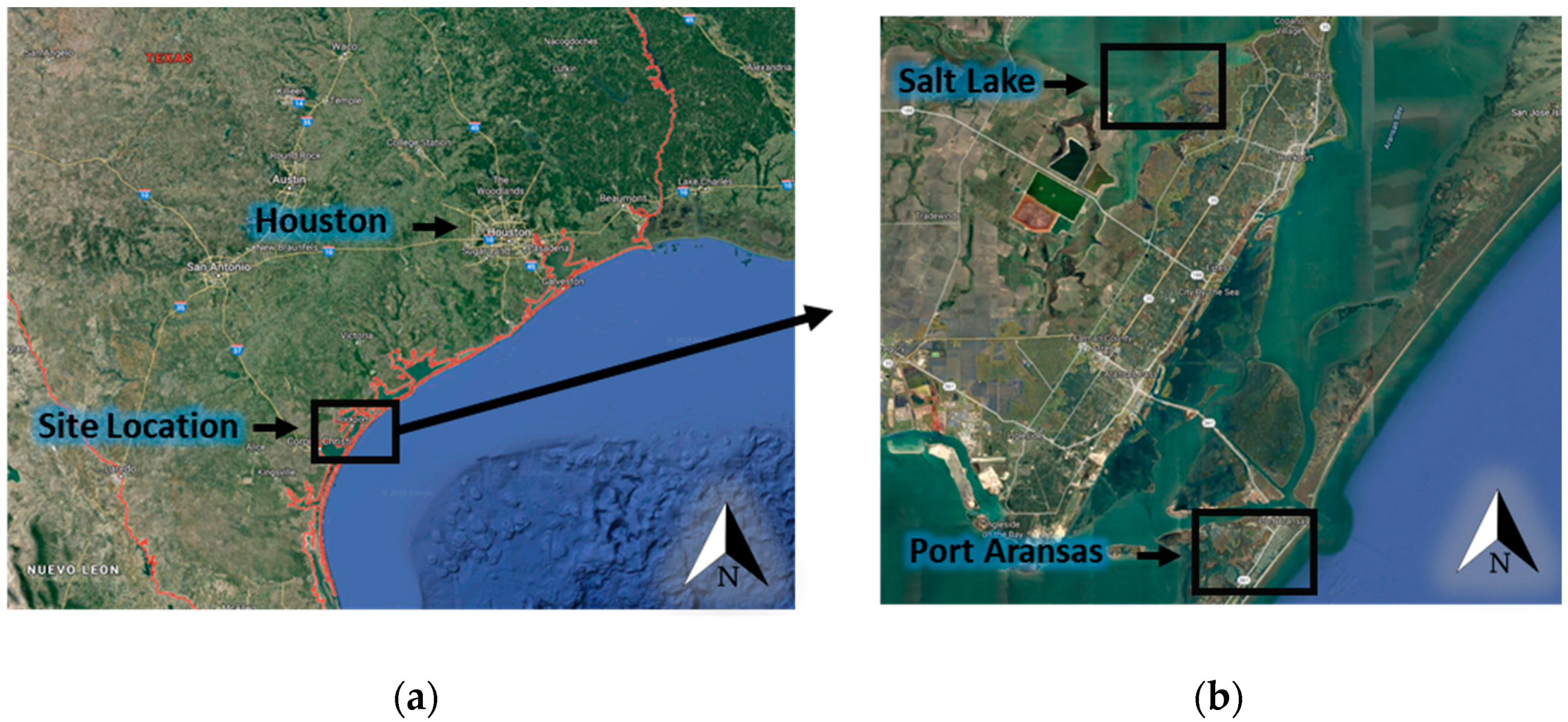
2.1. Introduction to Hurricane Harvey

On 25 August 2017, Hurricane Harvey struck the Texas coastline as a Category 4 hurricane making it the first major hurricane in 12 years to make landfall on the US mainland. Harvey produced wind gusts over 215 km/h (130 mph), and storm surges as high as 3.6 m (~12.0 ft) causing widespread damage to buildings and critical infrastructure in coastal communities including Rockport and Port Aransas [35]. Hurricane Harvey was responsible for the destruction of over 15,000 homes and damaged another 25,000 [38]. The storm’s 68 direct loss of lives in Texas made it the most detrimental hurricane to hit the state since 1919 and caused damage estimated at $125 billion, tying Hurricane Katrina, as the costliest US tropical cyclone in history [39].

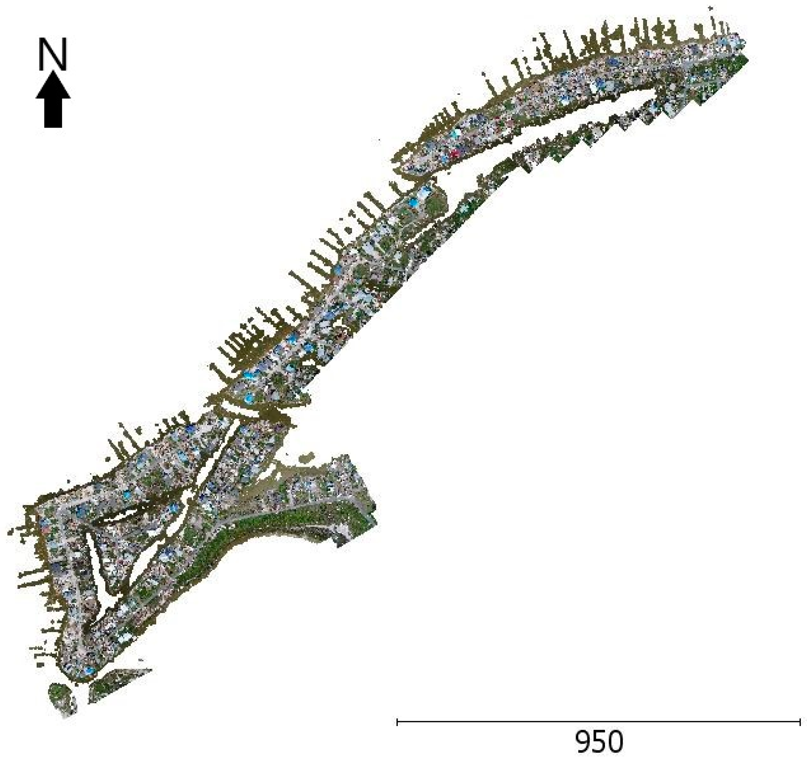
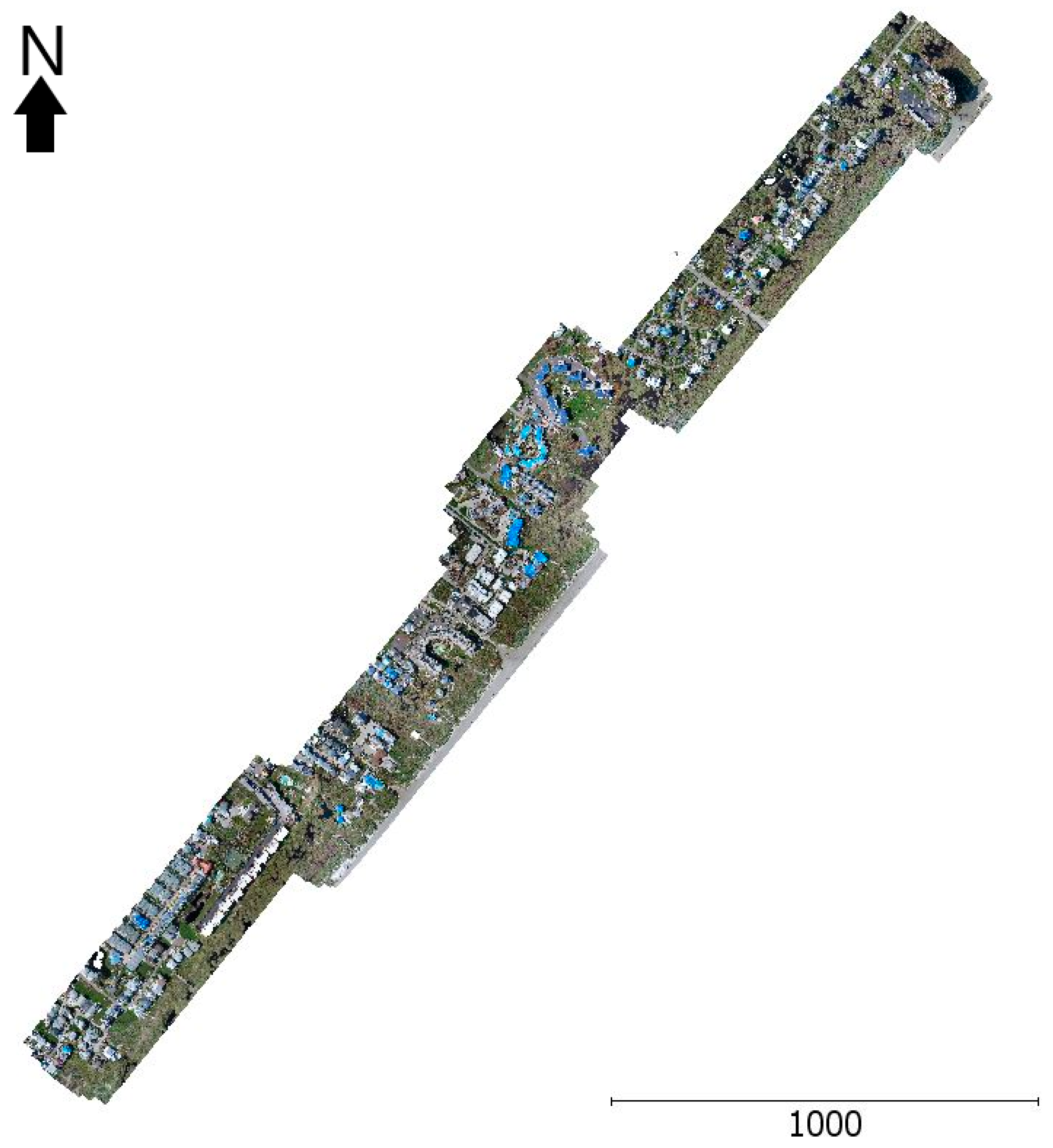
2.2. Data Collection Details

Kijewski-Correa et al. [40] coordinated a large reconnaissance effort to document the distribution and intensity of damage following the hurricane located along the Texas Coast. Within this group, a subset of researchers led by Professor Michael Starek of Texas A & M University-Corpus Christi conducted aerial data collection for a 0.88 km2 region of Port Aransas (approximately at a latitude of 27.8332 and a longitude of −97.0622) and a 0.73 km2 region of the Salt Lake neighborhood in Rockport (approximately at a latitude of 28.0229 and a longitude of −97.0551). The data was collected using a DJI Phantom 4 Pro drone at an altitude of approximately 91.5 m (300 ft) AGL. No ground control was available for these flights, therefore, the geolocation and scale are approximated by the onboard GPS on the UAS platform. The imagery datasets were processed by the authors of this study using Pix4Dmapper to produce the 3D point clouds. The average ground sampling distance (GSD) or the distance between pixel centers measured on the ground was approximately 2.7 cm for both datasets. The average density of the Salt Lake dataset is 172.2 points/m3 while the Port Aransas is 162.1 points/m3. The general locations of Salt Lake and Port Aransas are shown in Figure 1. Illustrated in Figure 2 is the Salt Lake point cloud, which is approximately 2350 m long by 310 m wide. Figure 3 displays the Port Aransas point cloud, which is approximately 3200 m long by 275 m wide.

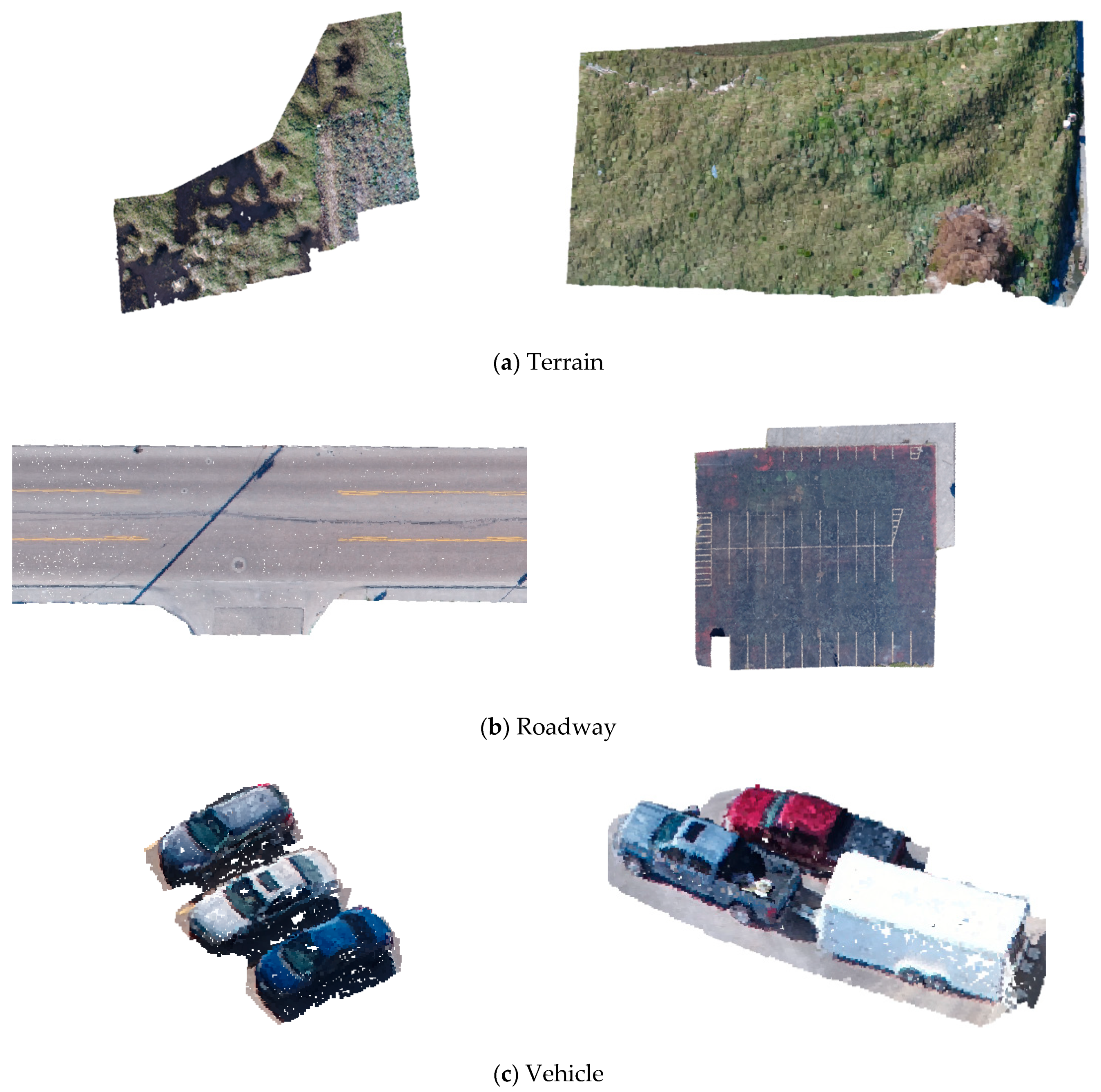
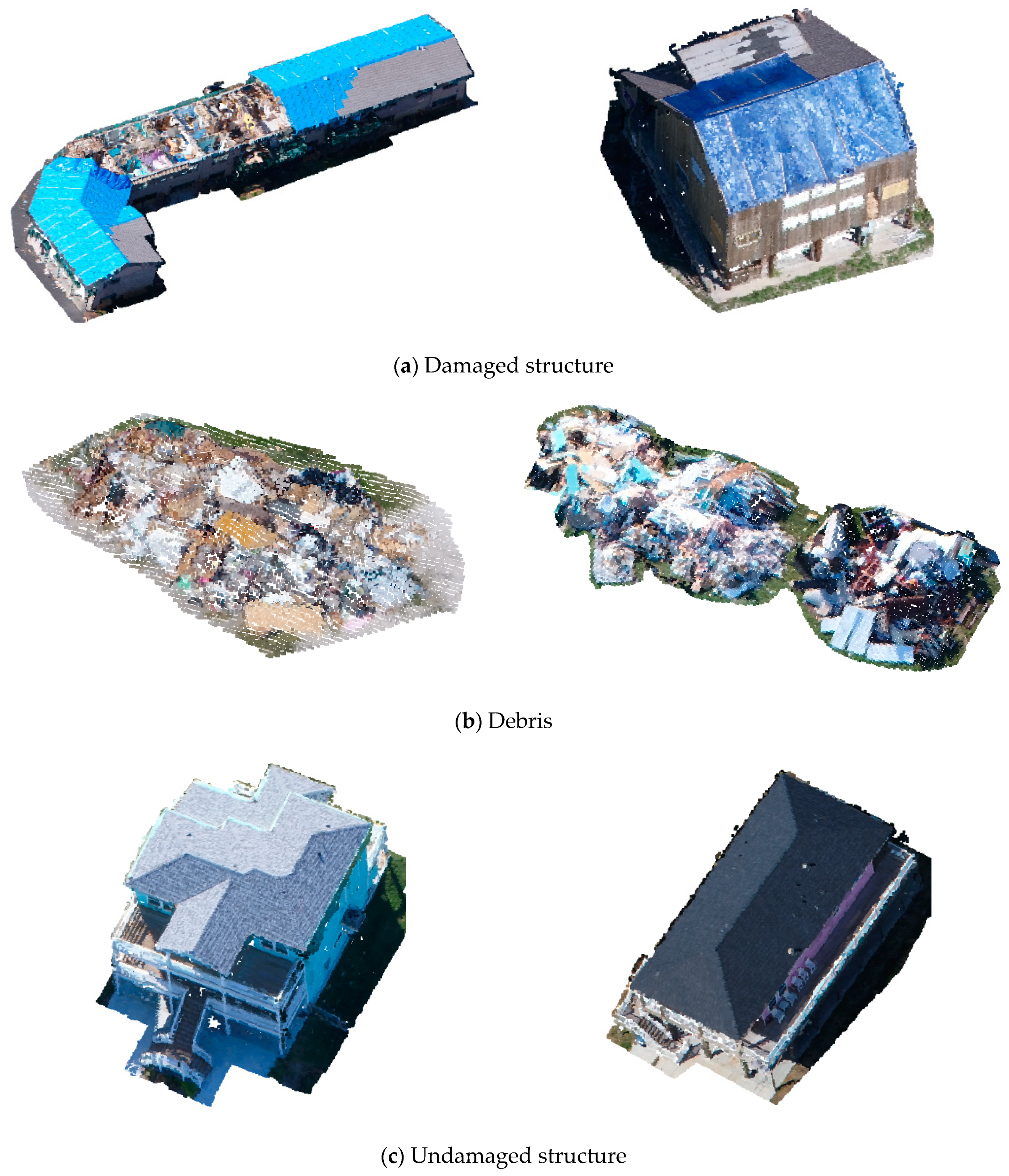
2.3. Dataset Classes

Each point cloud dataset was manually subdivided into one of the following six classes: vehicles, damaged structures, undamaged structures, debris, roadways, and terrain. For example, Figure 4 and Figure 5 demonstrate a few instances of each class. The vehicle classification broadly consists of anything used to transport people or goods such as a car, truck, cart, recreational vehicle (RV), trailer, construction vehicle (e.g., excavators, bulldozers), or any marine vessel that can be propelled on water by oar, sail, or engine. To classify structures, three different conditions are utilized: undamaged, damaged, and collapsed. A damaged structure includes any building structure that underwent physical changes due to the storm. Damaged structures range from minor to moderate damage such as roof damage with and without tarp coverings (tarps are typically blue in these data), to partially collapsed buildings. The partially collapsed structures still have visible structural components such as beams, columns, or walls. However, if a structure is completely collapsed or demolished with no identifiable structural components, the structure is classified as debris. Debris broadly contains anything not in its native state. This can consist of shingles from a rooftop, fallen trees, downed utility or light poles, and other wind-blown artifacts. On the contrary, undamaged structures are intact building and bridge structures that went through the event with no observed changes. Terrain encompasses any stretch of land consisting primarily of grass, low-height vegetation (bushes), water, sand, trees, exposed soil, fences, or utility poles. In this work, utility and light poles resemble a geometry similar to that of trees (consisted of predominantly cylindrical column) and are included as terrain due to their nonbuilding structural classification [41]. Roadways are classified as any prepared surface created specifically for transportation modes. This includes roadways, sidewalks, parking lots, and driveways made of gravel, asphalt, and concrete. Table 1 and Table 2 summarize the number of instances that were segmented for Salt Lake and Port Aransas, respectively. Note that the instances do not necessarily reflect the total unique count of the actual object. If a group of the same objects is close enough together, they are combined into one instance to include all possible situations in the training dataset. For example, if a group of eight trees is in close proximity, all eight trees were combined into a single instance of the terrain class.

3. Methodology

While aerial point cloud data provides a rich digital representation and view of the ROI, it also introduces a unique set of challenges in terms of scene classification. Specifically, this is due to its large number of points, point density variation, and more importantly, how various objects appear and maybe occluded due to nadir and obliques views. In addition, unordered and raw point clouds are unsuitable for use in high-performance and robust learning algorithms such as CNNs. As a result, the point cloud representations are converted into a volumetric grid model, where the object shape is represented as an occupancy grid, providing a suitable 3D representation to be used in CNN architecture. Using an occupancy grid representation of 3D objects introduces a series of difficulties including higher computational and spatial complexity as well as low resolution due to the voxelization process. However, recent advances within computational hardware, in particular GPUs with a large number of threads and global memory, provide the opportunity to develop CNN models based on 3D occupancy grids with a manageable amount of time and resolution. Therefore, within this study, a three-dimensional fully connected convolutional network (3D FCN) was developed based on two different occupancy grid resolutions of (64 × 64 × 64) and (100 × 100 × 100) to classify the vertices within the datasets for the post-windstorm damage assessment. This section initially describes the data preparation process to convert raw point cloud data into 3D occupancy grids, then presents the developed network architecture, and finally reviews the training strategy used to develop the two models.

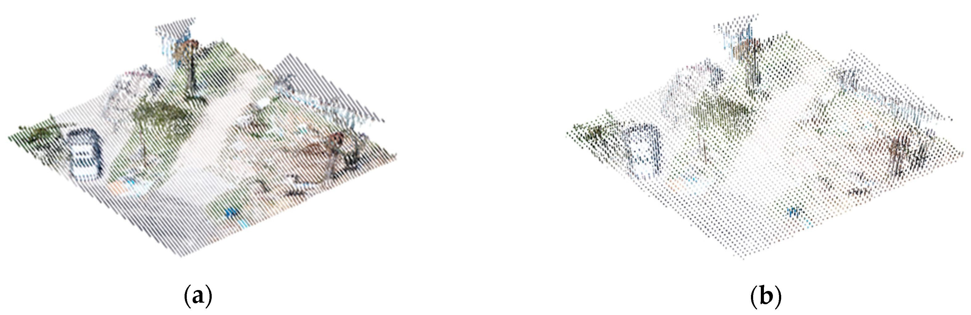
3.1. Data Preparation and Occupancy Grid Model

Data creation was initially performed by manually segmenting the aerial point clouds into the aforementioned six classes. Afterward, the labels corresponding to the objects are assigned to all the vertices within each segment, and the segments are then compiled into a single file. Then, the dataset is sliced into 10 × 10 m segments to create segments of equal dimensions that consist of multiple objects and multiple labels. In addition, and more importantly, the strategy in data preparation allows the user to control the data resolution. To create occupancy grid models based on each segment with multiple labels, initially the minimum value for each inputted instance component (i.e., x, y, and z) is calculated, and then the values are subtracted by the corresponding minimum values to transfer the data into positive ordinates. Afterward, the input dataset is downsampled based on the selected occupancy grid dimensions. Within this study, two occupancy grid sizes of 64 and 100 are selected, which result in a distance interval of 16 and 10 cm, respectively. This level of detail or resolution is suitable to perform a per building damage assessment for post-wind storm assessments [42]. To maximize the usage of the entire occupancy grid, the range for each component (i.e., x, y, and z) is computed and normalized. Finally, the values are multiplied by the selected dimension for the 3D grid model and rounded. Lastly, as each occupancy grid will have an amount of empty space (i.e., empty cells) as well as occupied spaces, an extra label corresponding to an empty space was added to the training labels known as neutral. Figure 6 illustrates a single instance along with its 3D occupancy grid representation in the described approach. Note, to preserve color information (i.e., RGB values), each training instance results in three occupancy grid representations corresponding to red, green, and blue color channels.

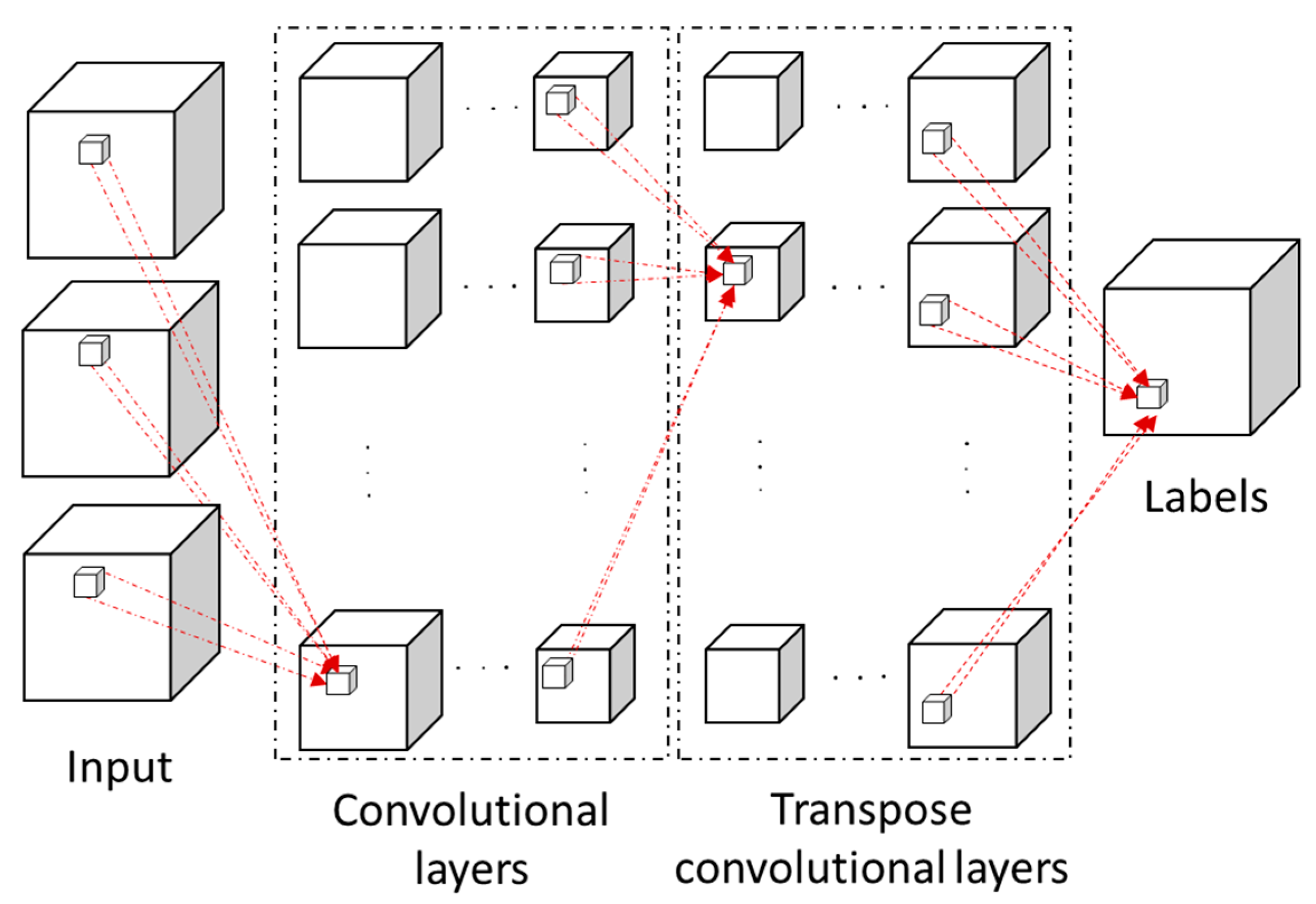
3.2. Three-Dimensional Fully Convolutional Network

In general and in deep learning, deep neural networks (DNNs) is a special instance of an artificial neural network (ANN), also known as a multilayer perceptron (MLP), that has significantly more learnable parameters. An ANN essentially represents a function, f, that consists of a set of weights and constant values, θ, that are organized in a structured pattern. The goal of an ANN is to approximate f such that it maps an input, such as x, to a label y. This can be represented mathematically using Equation (1):
y = f(x;θ),
where, θ is the set of weights and parameters that are also known as the learnable parameters. As Equation (1) demonstrates, the network accepts an input, x, to produce an output, y, through estimating or learning θ such that the y is minimized or correctly estimated. The training process updates the θ values through multiple iterations (or epochs) based on a loss function. The loss function measures the difference between predicted and true label values at each step of training, and the learning is performed by minimizing the loss function through methods such as stochastic gradient descent (SGD) and updating θ via a backpropagation algorithm [43]. CNNs are inspired by biological processes to improve computational efficiency in efficiently analyzing discrete and grid-like data (e.g., images, volumetric models) [4]. Within CNNs, the convolution operate is used (between convolutional layers) and weights and parameters are shared between each layer. CNNs can be trained similar to ANNs, but usually are comprised of convolutional layers as well as MLP layers to perform the prediction task [26]. However, and specific to this work, fully convolutional networks (FCNs) consist of convolutional and deconvolutional layers to enable identification at the point cloud’s vertex level.
The 3D FCN developed in this study is inspired by the previous work performed by Long et al. and Mei et al. [44,45]. In these previous studies, the researchers developed a 2D and 3D fully convolutional network for semantic segmentation of 2D images. Specific to the work presented in this manuscript, a 3D FCN was developed and implemented in TensorFlow v1.13. Herein, the developed 3D FCN is comprised of an input layer, convolutional layers, transpose convolutional layers, and an output layer (Figure 7). As shown, the input and output of the network at each step is a 3D grid model, which is similar to a 3D matrix. The learnable parameters within the presented networks are the weights that are used in the convolutional operations that reside in the dashed lines. The input layer accepts three grid models that correspond to the red, green, and blue channels. Afterward, the four convolutional layers convolve with the input occupancy grids in tandem and direct the results into four transpose convolutional layers that produce a grid model of the corresponding size of the input data with the predicted labels. All the convolutional and transpose convolutional layers have a total of eight filters. The filter sizes selected for the convolutional and transpose convolutional layers are set to minimal values (3 × 3 × 3) to reduce the number of parameters per layer and reduce the over-fitting potential risk. As shown in Figure 7, each small 3D grid that has an outbound arrow represents a (3 × 3 × 3) filter tensor which results in a (1 × 1 × 1) tensor (i.e., a cell of a larger 3D grid). The same padding and stride parameters of unity are used for all the layers. Therefore, each input and output layer of the convolutional and transpose convolutional layer is a four-dimensional tensor with a shape of (h × w × d × c), where h, w, and d, are spatial dimensions and c is the number of color channels. The output of each convolutional and transpose convolutional layer is thresholded by the rectified linear unit activation function [46], with a dropout value of 0.4. The 3D convolution operation is similar to that of 2D operations with the primary difference being that in 3D convolution and transpose convolution, the kernel can be imagined as a cube that slides in three directions (i.e., width, depth, and height) to construct the output [47]. Within the convolution operation, the elements are inputted with dimensions equal to kernel convolved to create an input of smaller dimension [45]. However, in the transpose convolution, the kernel is scaled by each input element separately to create intermediate results and then it slides based on the selected parameters. The output is created through a summation of the intermediate results [47].

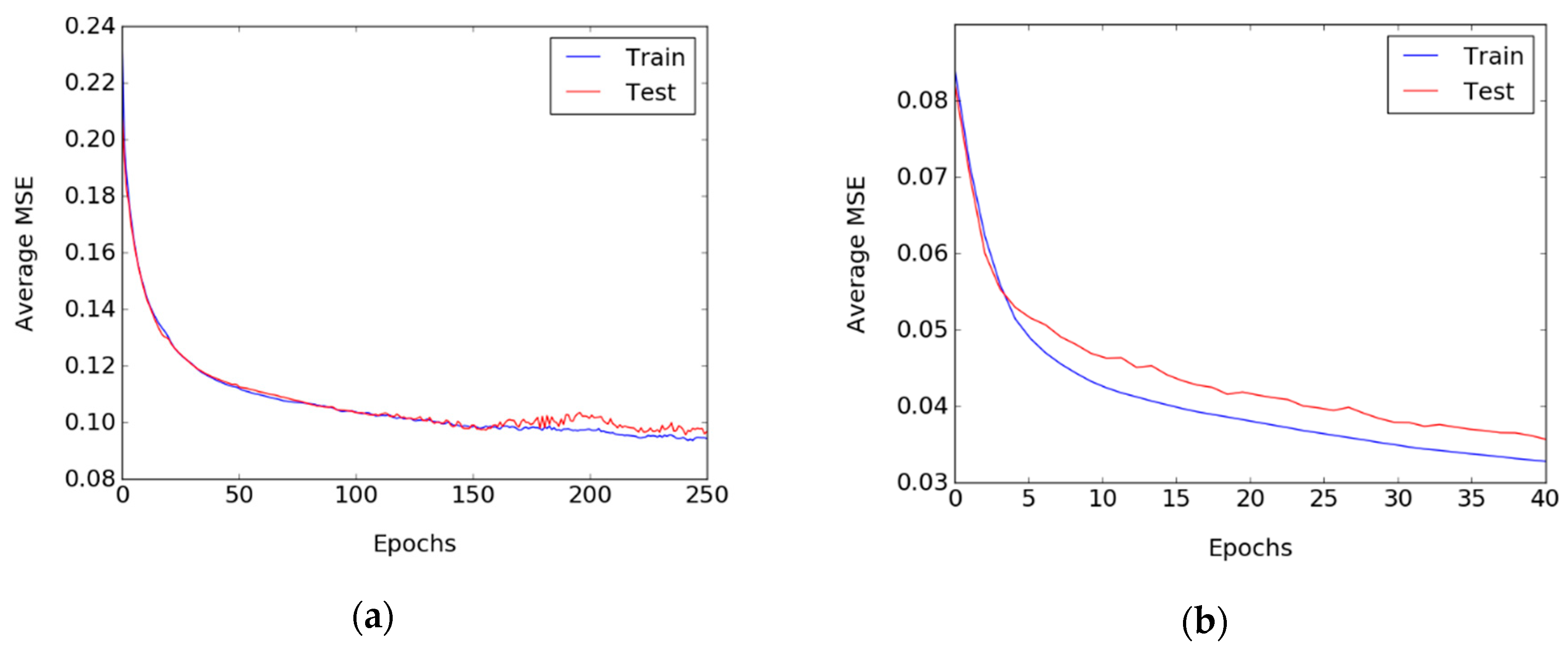
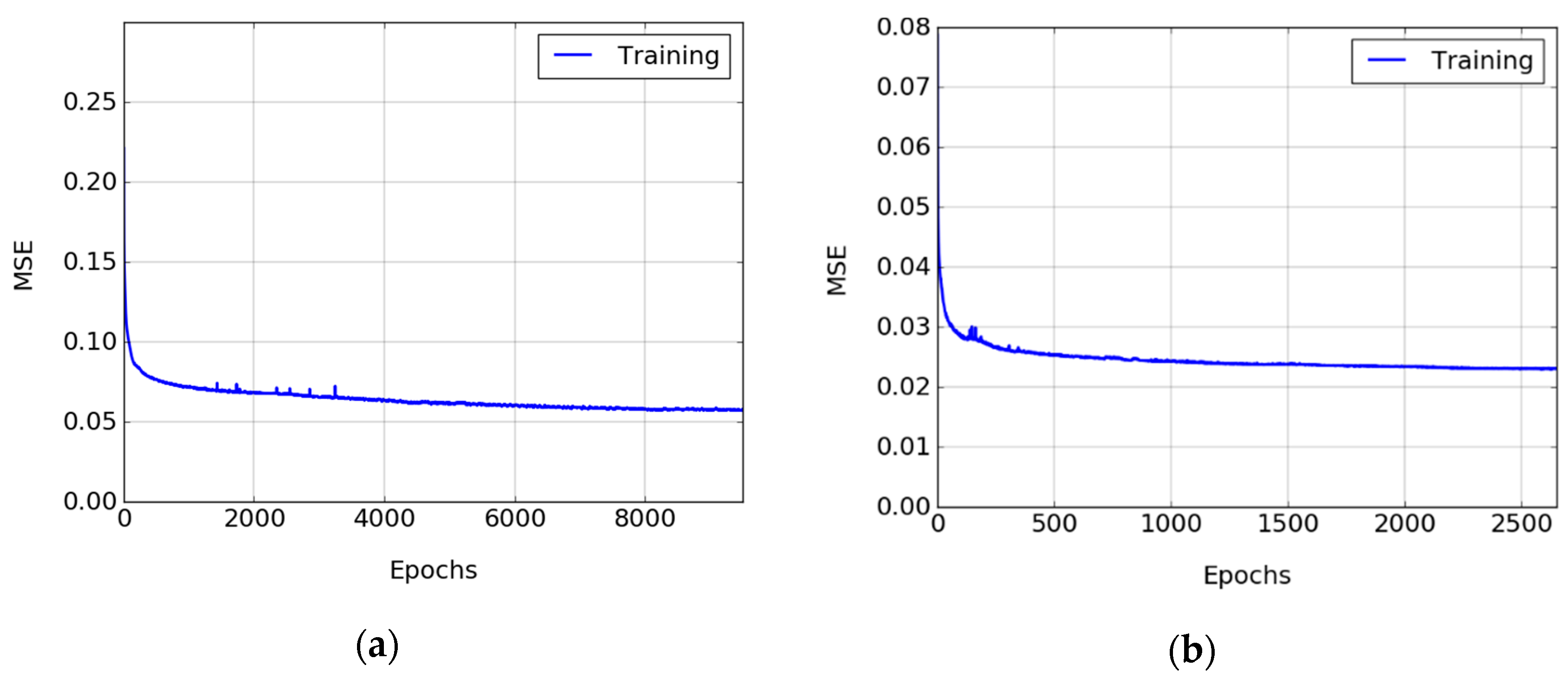
3.3. Training Process

The training process to develop a 3D FCN is similar to that of ANNs, DNNs, and CNNs. For the training, a real-valued loss function based on the mean squared error (MSE) is used. The MSE measures the differences between the corresponding elements of 3D FCN predictions and true labels. The network was optimized with the SGD. It was noted that a large number of empty cells exist in comparison to occupied cells, therefore, the location of occupied cells within the label was weighted by a factor of two during the training process to increase the learning rate within the targeted areas. To train and test the models, a minibatch size of 64 and 24 was used for the occupancy grids of size 64 and 100, respectively. The training focused on the Salt Lake dataset, and then the developed models were tested on Port Aransas instances with a corresponding resolution. The segmentation of Salt Lake instances with a grid size of (10 × 10) meters resulted in 5479 unique instances. However, with the sensitivity of 3D CNNs to orientation, as demonstrated by Sedaghat et al., the instances were randomly rotated twice along the global vertical axis to increase the network prediction capability [48]. In the end, the Salt Lake dataset comprised of a total of 10,958 instances, which were split into 80% for training (8766 instances) and 20% for testing (2192 instances), respectively. To develop the model, initially, the architecture was selected and trained based on the k-folds cross-validation process. This step was performed to ensure that the selected architecture and other hyperparameters can classify the input instances correctly. This included the number of convolutional layers, size of filters, stride, padding parameters, and selected loss function. Once the hyperparameters were selected, a model based on the entire 10,958 dataset instances was trained for an extended period of time to increase the model prediction performance.

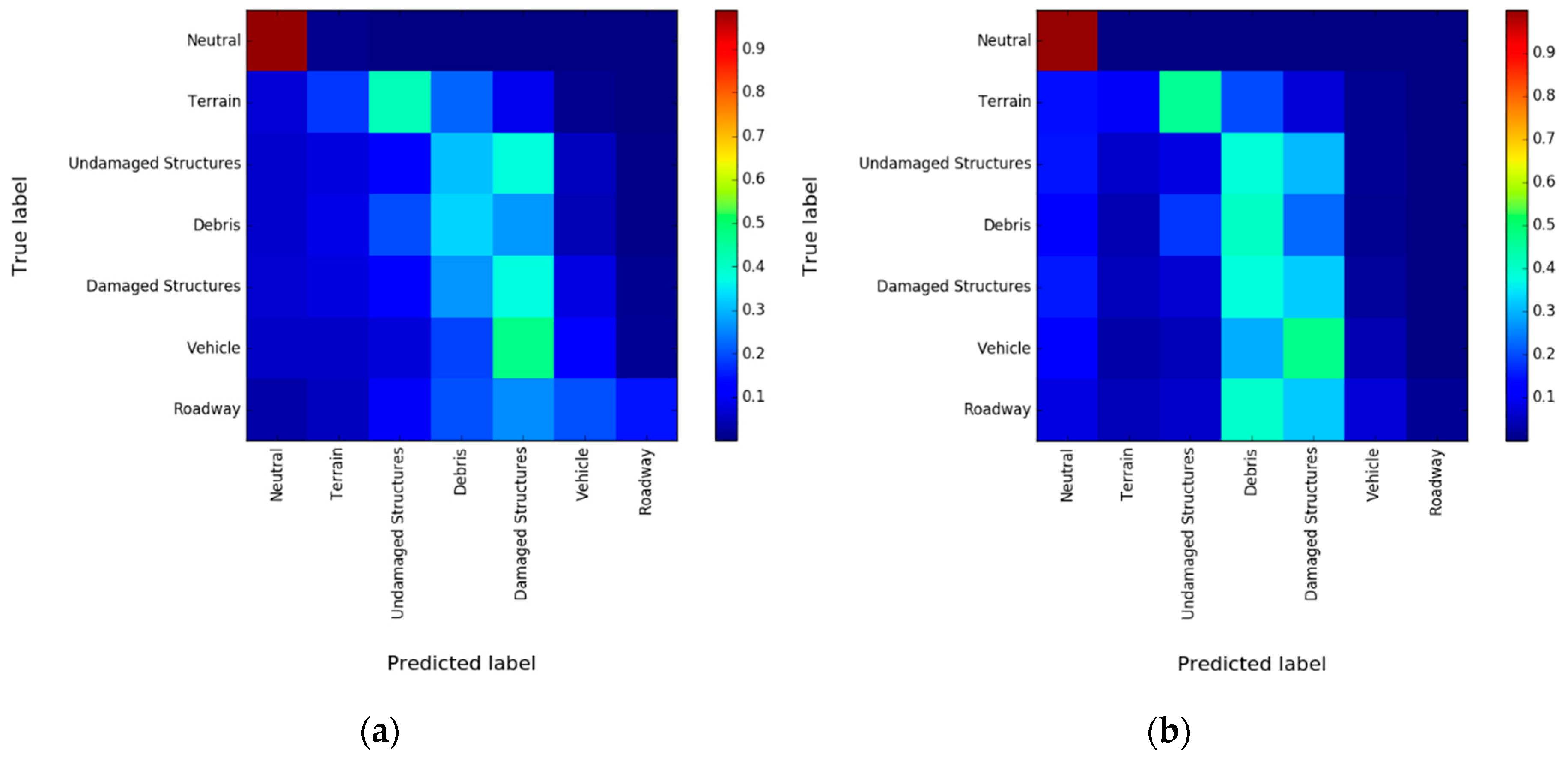
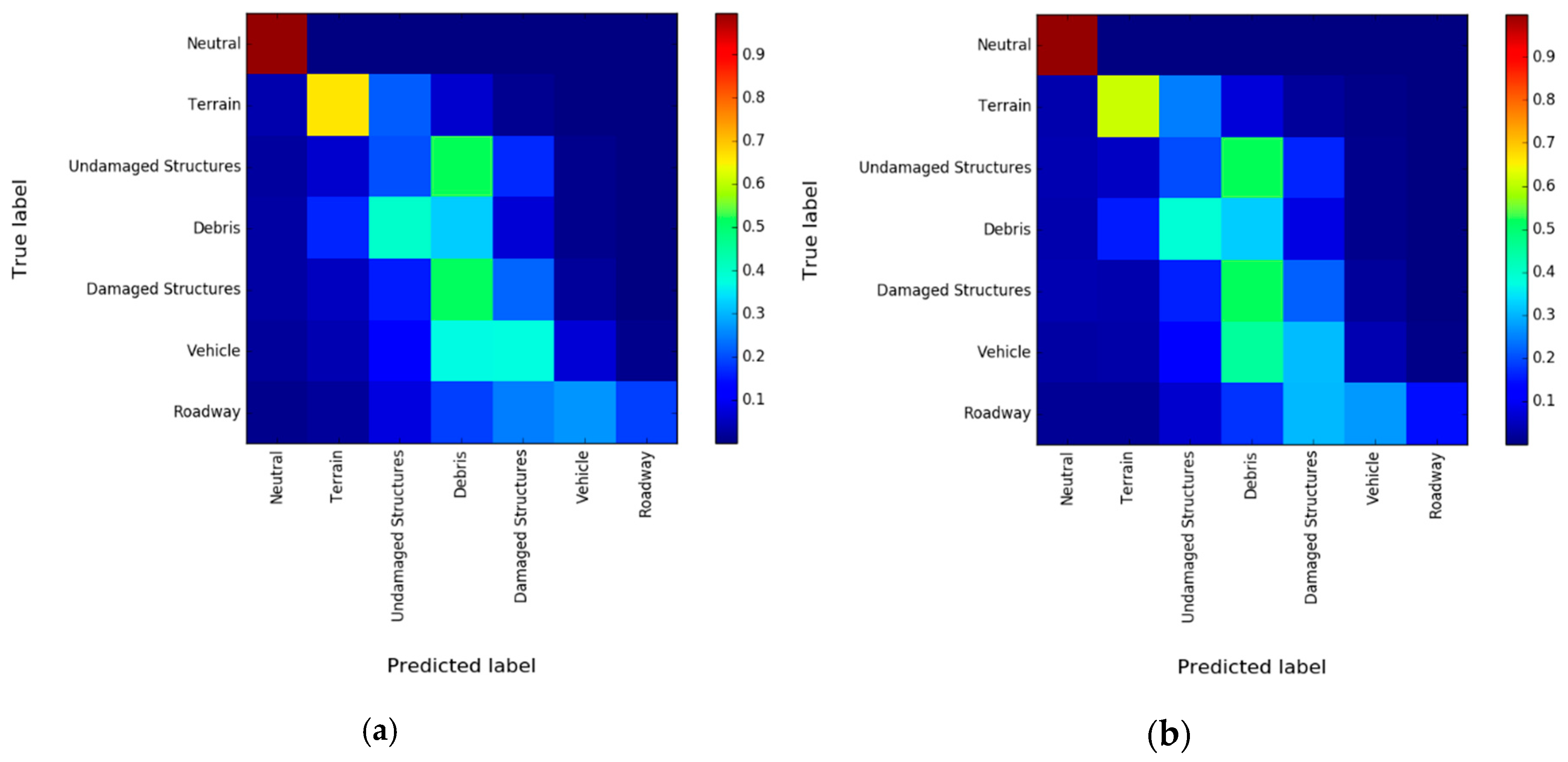
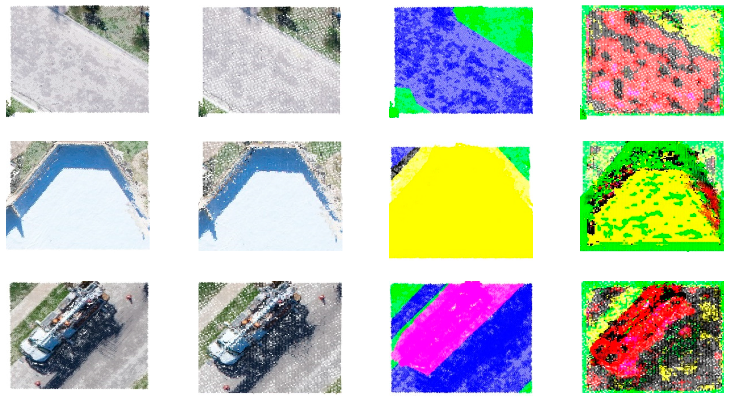
3.4. Experimental Results and Discussion

The developed models were trained primarily on the GPU resources at the Holland Computing Center, located at the University of Nebraska-Lincoln. Once the training was complete, the model was implemented for testing on the two datasets, Port Aransas, on a local machine. To measure the success of robustness of the developed network, a series of performance measures based on the confusion matrix (CM) is used including recall, precision, voxel accuracy, and intersection over union (IOU). The CM is square, of rank N, and comprises of c ij scalar values. The mentioned performance measures can be computed based on the equations below:
recall = C ii C ii + j i C ij
precision = C ii C ii + j i C ji
voxel   accuracy = C ii i j C ji
IOU = C ii C ii + j i C ji + j i C ij
where, c ii represents the diagonal CM elements and the true predictions, j i C ij represents the false negatives (upper triangle components, but not the main diagonal), j i C ji represents the false positive predictions (lower triangular components, but not the main diagonal), C ii denotes the total count of the true predictions, and i j C ji represents the total count of all predictions.
Two trained models focused on instances derived from the Salt Lake dataset. The initial MSE values of the trained model on the Salt Lake test set is presented in Figure 8. As the results of k-fold cross validation initially suggest (Figure 8), the MSE values demonstrate a steadily decreasing trend. Therefore, the models were further trained on the entire dataset for an extended time period to yield accurate results (Figure 9). The model based on resolution 64 occupancy grids (model-64) was trained for a total of 9500 epochs. On the contrary, the model based on 100 occupancy grids (model-100) was only trained for 2600 epochs, due to the higher computational demand of the model-100 as compared with the model-64. Figure 10 illustrates the CMs for the first and the second models developed based on the occupancy grid sizes of 64 and 100, respectively. Table 3 demonstrates the precision, recall, and IOU values for each class for both models. It is predicted that additional training epochs will result in significantly more accurate predictions and can match the results reported by current studies. Moreover, the performance and accuracy of the developed models cannot be directly compared with recent studies as the scope of this study was to classify all the vertices within the scene as compared to previous studies that only focused on classifying regions into two classes, damaged or undamaged [26]. The voxel accuracies for the model-64 and model-100 were 97.2%, and 97.6%, respectively. This high number is due to correct predictions of empty cells. This signifies that the developed models are able to predict the geometry of the input (filled cell distributions) instances with a high level of accuracy. As expected, model-100 demonstrates better precision throughout the various classes. This is due to the larger areas and the presence of more detailed geometric and color information, which aids in the ability to distinguish between classes.
To evaluate the trained 3D FCN models for transferability, the developed method was further tested on the Port Aransas dataset. Note that this dataset is completely independent of that of Salt Lake. While both are located on the southeast Texas Gulf Coast, the feature inventory is not identical due to the local geographical differences, as demonstrated in Figure 1. The Salt Lake community is located on an interior waterway, while Port Aransas is directly located on the gulf which results in differences in the feature inventory, due to the varying buildings, structures, and terrain (e.g., dunes). Feature inventory, in this sense, refers to the distribution and properties of the buildings, structures, and terrain which are of different sizes, shapes, and textures due to differences in the community’s location and population. In addition, and as discussed by Roueche et al., the level of damage sustained at each community varies [35]. The difference in feature inventory is important to highlight because what is learned during the training process may not cover every instance that occurs in the testing dataset (Port Aransas), leading to additional uncertainty. To prepare the Port Aransas dataset and quantitatively analyze the developed models, a label was assigned to each point (of the aforementioned six classes) and segmented into 10 × 10 meter instances. Port Aransas consist of 8776 instances, where the entire 100% is used for testing here, and the model is not retrained for the slightly different feature inventory. Figure 11 demonstrates the CMs for the two-occupancy grid resolution (model-64 and model-100), which demonstrates the classification results of trained models on the Port Aransas dataset. Table 4 demonstrates the precision, recall, and IOU values for each class for both models. The voxel accuracy for the model-64 and model-100 were 97% and 97.4%, respectively.
As demonstrated by the CM of each model and the quantified values presented in Table 4, the precision, recall, and IOU values identified for the Port Aransas dataset are slightly lower in comparison to the testing dataset results of Salt Lake. This reduced transferability is anticipated and a direct impact of the variations of the feature inventory in the two datasets. To visually demonstrate the performance of the developed models on the Port Aransas dataset, multiple segments of the dataset were selected and analyzed. The detailed view of each selected segment, along with the corresponding ground truth values and RGB colored point clouds, are shown in Figure 12 and Figure 13. Column (d) of Figure 12 and Figure 13 corresponds to prediction results of the model-100 and model-64, respectively. As demonstrated, the model-64 outperformed the model-100 in classifying roads and damaged structures. However, the model-100 was able to distinguish between structures (both damaged and undamaged structure classes) and nonbuilding structures, as shown by the second example of Figure 12 and Figure 13, whereas, the model-64 classified the instances predominately as debris. The results demonstrate that the model-100 still requires additional training to classify the classes roadway and debris from terrain and debris. The model-64 was able to demonstrate on par and better performance in detected structures from non-structures, while it demonstrates misclassification of other classes as the damaged structure class. Due to longer training, the model-64 demonstrates better learning of the less frequent classes like roadways than the model-100, as shown by the first instance presented in Figure 12 and Figure 13. The mediocre performance of the developed method is attributed to an insufficient number of training instances to represent objects that are more frequent in Port Aransas.

4. Conclusions

This study presents a 3D fully convolutional network (3D FCN) based on aerial point cloud data to semantically classify post-event scenes for forensic wind damage assessment and analysis. To develop the 3D FCN models, point cloud datasets were collected and created from two damaged sites at the south of Texas in the aftermath of Hurricane Harvey. These datasets were processed, a label was assigned to each of the vertices within these datasets, and finally were divided into (10 × 10) meter pieces. The 3D FCN models were developed based on two occupancy grid resolutions of (64 × 64 × 64) and (100 × 100 × 100) where each resulted in subsampling with sub-meter intervals. The models were trained based on one site (Salt Lake) and tested on the second dataset (Port Aransas) to investigate the developed model’s transferability.
As illustrated by the mean squared error of the training results, the developed models are robust to learn the features, however, the convergence was shown to be slower, primarily due to the number of learnable parameters. The models were able to learn and predict the correct labels of the neutral and terrain classes but demonstrated a lower precision and recall for objects with similar geometric and color features. The models were successful in their transferability to classify the objects of a different dataset without training, including the prediction of damaged structures at both resolutions (model-64 and model-100), with some limitations. It is anticipated that training the models for an extended period of time will continue to improve the accuracy, precision, recall, and IOU of both models.

Author Contributions

Data curation, M.E.M. and D.P.W.; formal analysis, M.E.M.; methodology, M.E.M.; project administration, R.L.W.; supervision, R.L.W.; validation, M.E.M. and D.P.W.; writing—original draft, M.E.M., D.P.W. and R.L.W.

Funding

No external funding directly supports this work.

Acknowledgments

This work was completed utilizing the Holland Computing Center of the University of Nebraska, which receives support from the Nebraska Research Initiative. Data was collected by Professor Michael Starek of Texas A & M at Corpus Christi and its availability is greatly appreciated by the authors, as published on the National Science Foundation’s Natural Hazards Engineering Research Infrastructure (NSF-NHERI) DesignSafe cyberinfrastructure.

Conflicts of Interest

The authors declare no conflict of interest. In addition, the funders had no role in the design of the study; in the collection, analyses, or interpretation of data; in the writing of the manuscript, or in the decision to publish the results.

References

  1. Nozhati, S.; Ellingwood, B.R.; Mahmoud, H. Understanding community resilience from a PRA perspective using binary decision diagrams. Risk Anal. 2019. [Google Scholar] [CrossRef]
  2. Brunner, D.; Lemoine, G.; Bruzzone, L. Earthquake damage assessment of buildings using VHR optical and SAR imagery. IEEE Trans. Geosci. Remote Sens. 2010, 48, 2403–2420. [Google Scholar] [CrossRef]
  3. Li, L.; Li, Z.; Zhang, R.; Ma, J.; Lei, L. Collapsed buildings extraction using morphological profiles and texture statistics—A case study in the 5.12 Wenchuan earthquake. In Proceedings of the 2010 IEEE International Geoscience and Remote Sensing Symposium, Honolulu, HI, USA, 25–30 July 2010; pp. 2000–2002. [Google Scholar]
  4. LeCun, Y. Generalization and network design strategies. In Connectionism in Perspective; Elsevier: Amsterdam, The Netherlands, 1989; Volume 19. [Google Scholar]
  5. Ji, M.; Liu, L.; Buchroithner, M. Identifying Collapsed Buildings Using Post-Earthquake Satellite Imagery and Convolutional Neural Networks: A Case Study of the 2010 Haiti Earthquake. Remote Sens. 2018, 10, 1689. [Google Scholar] [CrossRef]
  6. Li, Y.; Hu, W.; Dong, H.; Zhang, X. Building Damage Detection from Post-Event Aerial Imagery Using Single Shot Multibox Detector. Appl. Sci. 2019, 9, 1128. [Google Scholar] [CrossRef]
  7. Hansen, J.; Jonas, D. Airborne Laser Scanning or Aerial Photogrammetry for the Mine Surveyor; AAM Survey Inc.: Sydney, Australia, 1999. [Google Scholar]
  8. Javadnejad, F.; Simpson, C.H.; Gillins, D.T.; Claxton, T.; Olsen, M.J. An assessment of UAS-based photogrammetry for civil integrated management (CIM) modeling of pipes. In Pipelines 2017; ASCE: Reston, VA, USA, 2017; pp. 112–123. [Google Scholar]
  9. Wood, R.L.; Gillins, D.T.; Mohammadi, M.E.; Javadnejad, F.; Tahami, H.; Gillins, M.N.; Liao, Y. 2015 Gorkha post-earthquake reconnaissance of a historic village with micro unmanned aerial systems. In Proceedings of the 16th World Conference on Earthquake (16WCEE), Santiago, Chile, 9–13 January 2017. [Google Scholar]
  10. Szeliski, R. Computer Vision: Algorithms and Applications; Springer Science & Business Media: Berlin, Germany, 2010. [Google Scholar]
  11. Crandall, D.; Owens, A.; Snavely, N.; Huttenlocher, D. Discrete-continuous optimization for large-scale structure from motion. In CVPR 2011; IEEE: Piscataway, NJ, USA, 2011; pp. 3001–3008. [Google Scholar] [Green Version]
  12. Liebowitz, D.; Criminisi, A.; Zisserman, A. Creating architectural models from images. In Computer Graphics Forum; Wiley Online Library: Hoboken, NJ, USA, 1999; pp. 39–50. [Google Scholar]
  13. Wood, R.; Mohammadi, M. LiDAR scanning with supplementary UAV captured images for structural inspections. In Proceedings of the International LiDAR Mapping Forum, Denver, CO, USA, 23–25 February 2015. [Google Scholar]
  14. Lattanzi, D.; Miller, G. Review of robotic infrastructure inspection systems. J. Infrastruct. Syst. 2017, 23, 04017004. [Google Scholar] [CrossRef]
  15. Atkins, N.T.; Butler, K.M.; Flynn, K.R.; Wakimoto, R.M. An integrated damage, visual, and radar analysis of the 2013 Moore, Oklahoma, EF5 tornado. Bull. Am. Meteorol. Soc. 2014, 95, 1549–1561. [Google Scholar] [CrossRef]
  16. Burgess, D.; Ortega, K.; Stumpf, G.; Garfield, G.; Karstens, C.; Meyer, T.; Smith, B.; Speheger, D.; Ladue, J.; Smith, R. 20 May 2013 Moore, Oklahoma, tornado: Damage survey and analysis. Weather Forecast. 2014, 29, 1229–1237. [Google Scholar] [CrossRef]
  17. Womble, J.A.; Wood, R.L.; Mohammadi, M.E. Multi-Scale Remote Sensing of Tornado Effects. Front. Built Environ. 2018, 4, 66. [Google Scholar] [CrossRef]
  18. Rollins, K.; Ledezma, C.; Montalva, G.A. Geotechnical aspects of April 1, 2014, M 8.2 Iquique, Chile earthquake. In GEER Association Reports No. GEER-038; Geotechnical Extreme Event Reconnaissance: Berkeley, CA, USA, 2014. [Google Scholar]
  19. Vu, T.T.; Ban, Y. Context-based mapping of damaged buildings from high-resolution optical satellite images. Int. J. Remote Sens. 2010, 31, 3411–3425. [Google Scholar] [CrossRef]
  20. Olsen, M.J. In situ change analysis and monitoring through terrestrial laser scanning. J. Comput. Civ. Eng. 2013, 29, 04014040. [Google Scholar] [CrossRef]
  21. Rehor, M.; Bähr, H.; Tarsha-Kurdi, F.; Landes, T.; Grussenmeyer, P. Contribution of two plane detection algorithms to recognition of intact and damaged buildings in lidar data. Photogramm. Rec. 2008, 23, 441–456. [Google Scholar] [CrossRef]
  22. Shen, Y.; Wang, Z.; Wu, L. Extraction of building’s geometric axis line from LiDAR data for disaster management. In Proceedings of the 2010 IEEE International Geoscience and Remote Sensing Symposium, Honolulu, HI, USA, 25–30 July 2010; IEEE: Piscataway, NJ, USA, 2010; pp. 1198–1201. [Google Scholar]
  23. Aixia, D.; Zongjin, M.; Shusong, H.; Xiaoqing, W. Building Damage Extraction from Post-earthquake Airborne LiDAR Data. Acta Geol. Sin. Engl. Ed. 2016, 90, 1481–1489. [Google Scholar] [CrossRef]
  24. He, M.; Zhu, Q.; Du, Z.; Hu, H.; Ding, Y.; Chen, M. A 3D shape descriptor based on contour clusters for damaged roof detection using airborne LiDAR point clouds. Remote Sens. 2016, 8, 189. [Google Scholar] [CrossRef]
  25. Axel, C.; van Aardt, J.A. Building damage assessment using airborne lidar. J. Appl. Remote Sens. 2017, 11, 046024. [Google Scholar] [CrossRef]
  26. Vetrivel, A.; Gerke, M.; Kerle, N.; Nex, F.; Vosselman, G. Disaster damage detection through synergistic use of deep learning and 3D point cloud features derived from very high resolution oblique aerial images, and multiple-kernel-learning. ISPRS J. Photogramm. Remote Sens. 2018, 140, 45–59. [Google Scholar] [CrossRef]
  27. Weinmann, M.; Urban, S.; Hinz, S.; Jutzi, B.; Mallet, C. Distinctive 2D and 3D features for automated large-scale scene analysis in urban areas. Comput. Graph. 2015, 49, 47–57. [Google Scholar] [CrossRef]
  28. Hackel, T.; Wegner, J.D.; Schindler, K. Fast semantic segmentation of 3d point clouds with strongly varying density. ISPRS Ann. Photogramm. Remote Sens. Spat. Inf. Sci. 2016, 3. [Google Scholar] [CrossRef]
  29. Ji, S.; Xu, W.; Yang, M.; Yu, K. 3D convolutional neural networks for human action recognition. IEEE Trans. Pattern Anal. Mach. Intell. 2012, 35, 221–231. [Google Scholar] [CrossRef]
  30. Prokhorov, D. A convolutional learning system for object classification in 3-D LIDAR data. IEEE Trans. Neural Netw. 2010, 21, 858–863. [Google Scholar] [CrossRef]
  31. Weng, J.; Zhang, N. Optimal in-place learning and the lobe component analysis. In Proceedings of the 2006 IEEE International Joint Conference on Neural Network Proceedings, Vancouver, BC, Canada, 16–21 July 2006; IEEE: Piscataway, NJ, USA, 2006; pp. 3887–3894. [Google Scholar]
  32. Maturana, D.; Scherer, S. 3d convolutional neural networks for landing zone detection from lidar. In Proceedings of the 2015 IEEE International Conference on Robotics and Automation (ICRA), Seattle, WA, USA, 26–30 May 2015; IEEE: Piscataway, NJ, USA, 2015; pp. 3471–3478. [Google Scholar]
  33. Hackel, T.; Savinov, N.; Ladicky, L.; Wegner, J.D.; Schindler, K.; Pollefeys, M. Semantic3d. net: A new large-scale point cloud classification benchmark. arXiv 2017, arXiv:1704.03847. [Google Scholar] [CrossRef]
  34. Simonyan, K.; Zisserman, A. Very deep convolutional networks for large-scale image recognition. arXiv 2014, arXiv:1409.1556. [Google Scholar]
  35. Lombardo, F.; Roueche, D.B.; Krupar, R.J.; Smith, D.J.; Soto, M.G. Observations of building performance under combined wind and surge loading from hurricane Harvey. In AGU Fall Meeting Abstracts; American Geophysical Union: Washington, DC, USA, 2017. [Google Scholar]
  36. Roueche, D.B.; Lombardo, F.T.; Smith, D.J.; Krupar, R.J., III. Fragility Assessment of Wind-Induced Residential Building Damage Caused by Hurricane Harvey, 2017. In Forensic Engineering 2018: Forging Forensic Frontiers; American Society of Civil Engineers: Reston, VA, USA, 2018; pp. 1039–1048. [Google Scholar]
  37. Wurman, J.; Kosiba, K. The role of small-scale vortices in enhancing surface winds and damage in Hurricane Harvey (2017). Mon. Weather Rev. 2018, 146, 713–722. [Google Scholar] [CrossRef]
  38. Blake, E.S.; Zelinsky, D.A. National Hurricane Center Tropical Cyclone Report: Hurricane Harvey (AL092017); National Hurricane Center: Silver Spring, MD, USA, 2018. [Google Scholar]
  39. NHC Costliest U.S. Tropical Cyclones Tables Updated; National Hurricane Center: Silver Spring, MD, USA, 2018. [Google Scholar]
  40. Kijewski-Correa, T.; Gong, J.; Womble, A.; Kennedy, A.; Cai, S.C.S.; Cleary, J.; Dao, T.; Leite, F.; Liang, D.; Peterman, K.; et al. Hurricane Harvey (Texas) Supplement—Collaborative Research: Geotechnical Extreme Events Reconnaissance (GEER) Association: Turning Disaster into Knowledge. Dataset 2018. [Google Scholar] [CrossRef]
  41. The American Society of Civil Engineers (ASCE). Minimum Design Loads and Associated Criteria for Buildings and Other Structures; ASCE: Reston, VA, USA, 2016. [Google Scholar]
  42. Womble, J.A.; Wood, R.L.; Eguchi, R.T.; Ghosh, S.; Mohammadi, M.E. Current methods and future advances for rapid, remote-sensing-based wind damage assessment. In Proceedings of the 5th International Natural Disaster Mitigation Specialty Conference, London, ON, Canada, 1–4 June 2016. [Google Scholar]
  43. Rumelhart, D.E.; Hinton, G.E.; Williams, R.J. Learning representations by back-propagating errors. Cogn. Model. 1988, 5, 1. [Google Scholar] [CrossRef]
  44. Long, J.; Shelhamer, E.; Darrell, T. Fully convolutional networks for semantic segmentation. In Proceedings of the IEEE Conference on Computer Vision and Pattern Recognition, Boston, MA, USA, 7–12 June 2015; pp. 3431–3440. [Google Scholar]
  45. Mei, S.; Yuan, X.; Ji, J.; Zhang, Y.; Wan, S.; Du, Q. Hyperspectral image spatial super-resolution via 3D full convolutional neural network. Remote Sens. 2017, 9, 1139. [Google Scholar] [CrossRef]
  46. Nair, V.; Hinton, G.E. Rectified linear units improve restricted boltzmann machines. In Proceedings of the 27th International Conference on Machine Learning (ICML-10), Toronto, ON, Canada, 21–24 June 2010; pp. 807–814. [Google Scholar]
  47. Dumoulin, V.; Visin, F. A guide to convolution arithmetic for deep learning. arXiv 2016, arXiv:1603.07285. [Google Scholar]
  48. Sedaghat, N.; Zolfaghari, M.; Amiri, E.; Brox, T. Orientation-boosted voxel nets for 3d object recognition. arXiv 2016, arXiv:1604.03351. [Google Scholar]
Figure 1. Location of Salt Lake and Port Aransas datasets: (a) general location of both sites with respect to 239 major cities in southeast Texas and (b) detailed view of the regions where the Salt Lake community is located to the north and Port Aransas to the south (courtesy of Google Maps).
Drones 03 00068 g001
Figure 2. Salt Lake dataset (scale is in meters).
Drones 03 00068 g002
Figure 3. Port Aransas dataset (scale is in meters).
Drones 03 00068 g003
Figure 4. Example of instance existing in both Salt Lake and Port Aransas datasets.
Drones 03 00068 g004
Figure 5. Example of instances existing in both Salt Lake and Port Aransas datasets (continued).
Drones 03 00068 g005
Figure 6. Grid representation used within the dataset: (a) a segment consisting of objects in classes of vehicle, tree, debris, road, terrain, and undamaged structures and (b) the corresponding occupancy grid representation with voxel sizes of (64 × 64 × 64).
Drones 03 00068 g006
Figure 7. The developed 3D fully convolutional network (3D FCN) pipeline.
Drones 03 00068 g007
Figure 8. Average MSE of k-folds on Salt Lake tests: (a) model-64 and (b) model-100.
Drones 03 00068 g008
Figure 9. The mean squared error (MSE) during model training on the Salt Lake training datasets: (a) model-64 and (b) model-100.
Drones 03 00068 g009
Figure 10. Confusion matrices of the models trained on the Salt Lake testing results: (a) model-64 after 9500 epochs of training and (b) model-100 after 2600 epochs of training.
Drones 03 00068 g010
Figure 11. Confusion matrices of the testing results on the Port Aransas: (a) model-64 and (b) model-100.
Drones 03 00068 g011
Figure 12. The test-only results on the Port Aransas segments with an occupancy grid resolution of (100 × 100 × 100): (a) RGB original point cloud (top view); (b) subsampled RGB point cloud; (c) ground truth labels; and (d) predicted labels after 2600 epochs. Note the subfigure parts are shown in columns for four segments.
Drones 03 00068 g012aDrones 03 00068 g012b
Figure 13. The test-only results on the Port Aransas segments with an occupancy grid resolution of (64 × 64 × 64): (a) RGB original point cloud (top view); (b) subsampled RGB point cloud; (c) ground truth labels; and (d) predicted labels after 9500 epochs. Note the subfigure parts are shown in columns for four segments.
Drones 03 00068 g013
Table 1. Summary of instances for Salt Lake.
Instance# of InstancesPercentage of Total (%)
Damaged structures24213.4
Debris38621.3
Roadway573.2
Terrain71939.8
Undamaged structures1488.2
Vehicle25614.2
Total1808100
Table 2. Summary of instances for Port Aransas.
Instance# of InstancesPercentage of Total (%)
Damaged structures16210.0
Debris25515.7
Roadway875.3
Terrain66540.9
Undamaged structures23514.4
Vehicle22313.7
Total1627100
Table 3. The quantified performance measures on Salt Lake testing datasets for both models.
InstanceModel-100 (%)Model-64 (%)
PrecisionRecallIOUPrecisionRecallIOU
Neutral10010010010010099
Terrain816154736654
Undamaged structures52145204
Debris253317263317
Damaged structures282214312215
Vehicle442774
Roadway911414921918
Table 4. The quantified performance measures on the Port Aransas dataset for two models.
InstanceModel-100 (%)Model-64 (%)
PrecisionRecallIOUPrecisionRecallIOU
Neutral1001001001009999
Terrain32108321813
Undamaged structures4832112
Debris44143333
Damaged structures153212163713
Vehicle2412122
Roadway8322891514

