Abstract
Sugarcane products contribute significantly to the Brazilian economy, generating U.S. $12.2 billion in revenue in 2018. Identifying and monitoring factors that induce yield reduction, such as weed occurrence, is thus imperative. The detection of Bermudagrass in sugarcane crops using remote sensing data, however, is a challenge considering their spectral similarity. To overcome this limitation, this paper aims to explore the potential of texture features derived from images acquired by an optical sensor onboard anunmanned aerial vehicle (UAV) to detect Bermudagrass in sugarcane. Aerial images with a spatial resolution of 2 cm were acquired from a sugarcane field in Brazil. The Green-Red Vegetation Index and several texture metrics derived from the gray-level co-occurrence matrix were calculated to perform an automatic classification using arandom forest algorithm. Adding texture metrics to the classification process improved the overall accuracy from 83.00% to 92.54%, and this improvement was greater considering larger window sizes, since they representeda texture transition between two targets. Production losses induced by Bermudagrass presence reached 12.1 tons × ha−1 in the study site. This study not only demonstrated the capacity of UAV images to overcome the well-known limitation of detecting Bermudagrass in sugarcane crops, but also highlighted the importance of texture for high-accuracy quantification of weed invasion in sugarcane crops.
1. Introduction
Sugarcane is mainly cultivated in tropical and subtropical regions around the world, and is one of the most important sources of sugar and raw material for ethanol production [1]. Brazil is the world’s leading producer of sugarcane, with an estimated raw production of 641 million tons in 2018 [2]. This production supports the manufacturing of 38.6 million tons of sugar-related products and 27.8 billion liters of ethanol [2]. These numbers can be translated into annual exportation revenue of 12.2 billion dollars for the Brazilian economy [2]. Over the last 20 years, the planted area of sugarcane in Brazil has increased from 4.8 to 10.2 million hectares. Plantations in São Paulo state account for 55% of the entire Brazilian production [3]. To be able to maintain a high productivity of this crop, it is critical to constantly monitor climatic (e.g., rainfall and temperature), environmental (e.g., soil quality), and biological (e.g., weeds) factors that may reduce production.
Weed detection and control is especially important for achieving high crop yields. Weeds compete with sugarcane plants for water, nutrients, and sunlight, negatively impacting sugarcane growth. Abnormal weed growth can also interfere with some agricultural practices, including soil management and the use of herbicides, which can add extra labor and increase the overall cost of production [4]. Weeds are also pointed to as a host for sugarcane diseases and can contribute to pest infestations, such as the ground rat (Rattus sordidus), the cane beetle (Dermolepida albohirtum), and several nematode species [4,5,6,7,8].
There are a huge variety of weeds capable of infesting sugarcane crops. Some are dicotyledonous (usually called broadleaf weeds), but most are monocotyledonous and belong to the Poaceae family (commonly known as grasses) [4]. Weeds such as Cynodon dactylon (bermudagrass), Sorghum halepense (johnsongrass), Eleusine indica (goosegrass), Panicum maximum (guineagrass), and Brachiaria reptans (creeping panic grass) are highlighted as the most common species affecting sugarcane crops around the world [4,9,10,11]. In an experimental analysis of sugarcane crops without weed control, weeds affected up to 60% of the planted area, representing yield losses up to 45 tons × ha−1 [4]. Bermudagrass is responsible for yield losses that range from 6% to 14% of production (depending on the chemical control used), and is more critical in the early growth stages of a culture, as it shades emerging sugarcane shoots [9].
One way to effectively monitor weeds is using remote sensing data, especially those obtained by unmanned aerial vehicles (UAVs). These images are suitable for mapping areas where weeds have escaped control due to management errors or herbicide resistance [12]. UAV images capture the spectral reflectance of vegetation and other objects from above, reducing the time required for and the number of field campaigns necessary to investigate weed occurrence. Each object spotted by an airborne sensor has specific reflectance characteristics for each wavelength of the electromagnetic spectrum, which allows distinguishing them with image processing techniques. The spectral reflectance detected by each sensor’s channel (or band) is the baseline for applications involving weed mapping and airborne sensors [12,13].
Besides the spectral reflectance, image processing techniques provide other reliable products to improve weed detection, such asvegetation indices (VIs), for example [14]. VIs were developed to decrease data dimensionality and highlight objects with green vegetation. For airborne sensors, which usually have only red, green and blue (RGB) bands, VIs can be calculated based on the green (500–570nm) and red (620–700nm) regions of the electromagnetic spectrum [14]. It is known that the overall accuracy of weed mapping can be improved by using VIs derived from remote sensing data [15,16,17,18]. These VIs are capable of distinguishing vegetation parameters such as color, dry matter (%), nitrogen (%), chlorophyll (A and B), and carotenoid content among several varieties of grasses, such as Lolium perenne (perennial ryegrass) and Poa pratensis (kentucky bluegrass) [12]. However, for Bermudagrass, just spectral reflectance and VIs have not been enough to estimate these parameters precisely [12,13].
Potentially, the use of texture metrics derived from remote sensing images can improve weed detection [19,20]. A methodology using not only VIs, but also texture features, was developed in order to map weeds on maize and sunflower crops [15]. The authors used a 1.4-cm spatial resolution UAV image obtained from an RGB camera. After orthomosaic generation, they evaluated two classification strategies, the first one using only the RGB values and the second one considering features such as VI and texture. They used the support vector machine (SVM) algorithm for classification, and feature selection was performed with the “Information Gain” method on WEKA software [21,22]. When considering weed detection in sunflower crops, the overall accuracy (OA) using only the RGB band values was 61.6%, but when the second strategy was used, the accuracy values increased to 95.5%. The accuracy of weed detection in maize crops, on the other hand, had a lower performance, reaching a maximum OA value of 79.0% [15].
The combinationof VIs with texture features has also improved the OA of weed detection in eggplant plantations [16]. Using 5-cm spatial resolution images and the SVM classifier, the authors could not distinguish weeds from eggplants using nine different VIs (OA of 58.4%). By adding texture features to the dataset, these authors increased the OA of their classification to 75.4%. Differently from Reference [15], no feature selection method was applied to the dataset.
Another example was weed detection in bean and spinach crops [17]. The authors used a 0.35-cm UAV image obtained from an RGB sensor and compared the performance of three different classifiers (SVM, random forest [23], and convolutional neural networks (CNNs) [24]) with and without texture features. Similarly to References [15] and [16], the combined use of spectral values, VIs, and texture features obtained better results. For weed detection in bean crops, random forest outperformed the SVM classifier, with an OA of 70.1% against 60.6%. However, the best classification result was achieved by using CNNs, with an OA of 94.8%. For spinach crops, the random forest algorithm had better results than the other classifiers, with an OA of 96.9%.
An approach using image segmentation and object-based image analysis (OBIA) to discriminate crops and weeds was used by References [15] and [16]. Several segmentation approaches, such as the ones used by the authors, are based on spectral information similarity (usually a region growth algorithm) in order to develop the polygons used to separate the classes. On the other hand, weeds and crops are hard to discriminate between using only spectral information, considering their strong similarities [12,13,17]. Thus, applications that want to perform analyses on how texture influences weed detection can be performed applying a pixel by pixel strategy showing how texture window size influences classification results.
The use of texture and UAV images has the potential to improve the detection of weeds on a large variety of crops. Nevertheless, this combination has not yet been tested for sugarcane crops. In this sense, RGB UAV images have been used to identify Digitaria insularis (sourgrass) and Tridax procumbens (tridax daisy) [1]. The authors used statistical descriptors for pixel groups, such as mean, standard deviation, and variance, to classify three different classes (sourgrass, tridax daisy, and sugarcane plants). The OA using the random forest classifier and a cross-validation method was 77.9% and 85.5% for the sourgrass and tridax daisy, respectively. When the error matrix was analyzed, the sourgrass was misclassified as both sugarcane and tridax daisy, resulting in a commission error of 23.7%. For the tridax daisy, this error was 17.4%, and it was also misclassified as sugarcane.
A similar methodology has been used to identify sugarcane plants, soil patches, Lepidium virginicum (peppergrass), Nicandra physalodes (shoo-fly plant), and Brachiaria decumbens (signalgrass) [25]. The authors, using the same statistical descriptors as Reference [1], evaluated three different classifiers, and random forest and artificial neural networks (ANNs) obtained the best results [26]. The OA obtained by random forest was 90.9%, and for the ANNs it was 91.6%, where the main source of error was the misclassification between sugarcane and shoo-fly plants. However, no validation was described by the authors, and their results had higher OA values compared to Reference [1].
Multispectral UAV images (with 13 bands) have been used to map sugarcane plants affected by the mosaic virus (Potyviridae family), which is responsible for stunning plant growth due to mottling the laminar region of the plants and causing the discoloration of leaves [27]. The authors also mapped spots with Digitaria horizontalis (crabgrass) and guineagrass. An automatic classification was realized using the spectral information divergence (SID) algorithm, which uses only spectral reflectance [28]. The OA of the study was 92.5%, and hyperspectral images could separate healthy from infected plants. Regarding weed mapping, the authors mentioned it was difficult to identify theseweeds once the sugarcane plants were in an advanced growth stage and usually covered the weeds. Once again, VIs and texture features were not used for classification.
Lastly, RGB UAV images have been used to map the level of infestation of Bermudagrass in vineyards [18]. Using spectral reflectance and VIs with a region-basedclassification algorithm, the authors obtained an OA of 83.3%. However, they suggested that texture features may improve the results.
The potential of UAV images to detect Bermudagrass in sugarcane plantations has not been fully explored before, since other applications have not used both vegetation indices and texture features. In this context, the aim of this paper is to explore the potential of texture features and UAV images to detect bermudagrass occurrence in sugarcane crops in Brazil.
2. Materials and Methods
2.1. Study Site and Image Acquisition
The study site was in the Iracema Mill, located in São Paulo State, Brazil (Figure 1a). The Iracema Mill has been manufacturing sugarcane products such as sugar and ethanol for over 70 years, processing an average of 3 million tons of prime mater per year in an areaof 30,000 ha, spread across different municipalities of São Paulo State. Our study site was located in the Iracemápolis municipality (Figure 1b), which had 8,834 ha of planted crops, with sugarcane representing 95% of this area and being the most important source of income [3].
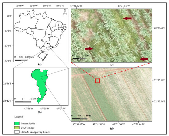
Figure 1.
(a) Location of the study site in São Paulo State, Brazil; (b) Iracemápolis municipality and the location where the image was acquired; (c) zoom representing the infestation of Bermudagrass (highlighted with red arrows) in a sugarcane field (gramineous weed between and within crop rows); (d) red, green, and blue (RGB) unmanned aerial vehicle (UAV) image of true color composition and 2-cm spatial resolution.
The area mapped was a heterogeneous sugarcane field (Figure 1d), with several planting failures and sugarcane plants in different growing stages (crown diameter ranging from 0.5 m to 2.0 m). The majority of the soil area was covered by sugarcane straws, but some spots were left uncovered. There were also a few flooded soil spots in small depressions, probably caused by the use of heavy machinery, and areas infested by Bermudagrass (Figure 1c).
Images were acquired on 16 February 2016, using a multirotor GYRO 200 OCTA 355 UAV (octocopter) equipped with a Sony RX100M3 camera of 20.1 megapixels and a CMOS Exmor R® sensor (RGB) (Figure 2). A gimbal was used to guarantee the acquisition of images with a nadir configuration, minimizing the effects related to variations in the platform altitude.
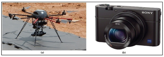
Figure 2.
(a) Octocopter GYRO 200 OCTA 355 UAV; (b) Sony RX100M3 camera of 20.1 megapixels.
Two flights were carried out in the study site, one at 10:00 and the other at 11:50, obtaining 153 and 135 images, respectively. These flights were realized during their respective hours due to a cloud-free sky. All images were acquired with an overlap of 80% (longitudinal) and 60% (side), with a flight height of 80m. This configuration resulted in a pixel size of 2cm. After image acquisition, an orthomosaic was generated using Pix4D software. Furthermore, the image was cropped in order to avoid low overlapping areas on the borders, resulting in the image presented in Figure 1d.
2.2. Feature Extraction
Using the orthomosaic, the Green-Red Vegetation Index (GRVI) was calculated [14]. A GRVI is used to highlight vegetation pixels considering the equation described below:
The GRVI ranges from −1 to +1, and the digital number (DN) values ofthe green and red bands were used for the index calculation. This index was selected, among others, because of its capability of detecting early phase or leaf green-up, which was suitable to the study site plant heterogeneity, and also because it is suitable for different ecosystem types [13,14,15,16].
The texture features were calculated for each RGB band and also for the GRVI image (7 textures per layer, i.e., 28 features). These features were computed from the gray-level co-occurrence matrix (GLCM), which is a second-order histogram where each entry reports the joint probability of finding a set of two gray-level pixels at a certain distance and direction from each other over a predefined window [19,20]. This window is shifted around the image, calculating the texture for each center pixel. It can be calculated for 4 different directions (0°, 45°, 90°, and 135°). In this study, the direction 0°was chosen, considering our image characteristics and class distribution [20]. This direction explores the texture from left to right, parallel to the horizontal axis, andcaptures the heterogeneity between crop rows, where weeds are usually located [9]. The window sizes used were 3 × 3, 5 × 5, 7 × 7, 9 × 9, 11 × 11, 13 × 13, and 15 × 15 pixels. These features were also used in other weed detection applications [15,16,17]. The texture metrics were calculated using the equations described below.
Pi,j is the normalized value for the cell i,j;N is the number of rows or columns; and µi,j is the GLCM mean.
Every GLCM generated is normalized to express the results into a close approximation of a probability table, according to the following equation [19,20]:
Vi,j is the value for the cell i,j of the matrix.
2.3. Classification
The classification algorithm used was random forest [23], which has presented good results in other applications using UAV images and weed detection [1,17,25]. The random forest algorithm is also considered computationally efficient and less sensitive to noisy data, and the generation of multiple trees with the bootstrap technique can also avoid overfitting [23,29]. The classification was performed pixel by pixel, and the algorithm was trained on 2000 samples for each of the five classes presented in Table 1.

Table 1.
The five classes used in this study.
The random forest algorithm has 3 parameters that need calibration: Tree depth, a number of random features selected for each node, and the number of trees. The trees were generated without pruning (tree depth is unlimited), the number of random features at each node is described by the equation below, and the number of trees was set to 1.000 [22,23]:
where total_features is the total number of features in the dataset, and Number of features on each node is rounded to the nearest integer.
A total of 8 experiments were realized to evaluate how texture contributes to weed detection. The first one was performed using only 4 features, the DN values for each RGB band and the GRVI. After that, for each window size, 28 texture features were calculated. For experiment 2, for example, the red, green, blue, GRVI, and 7 textures for each layer were used, resulting in a total of 32 features (4 + 7 × 4). The window size used for experiment 2 was 3 × 3. The same procedure was realized for further experiments, considering greater window sizes. For example, experiment 3 used 28 textures calculated from the 5 × 5 window and also the RGB and GRVI. This extended until experiment 8, which used textures calculated from the 15 × 15 window. Experiments 2 to 8 used a total of 32 features each.
Model validation was performed by the random selection of 2500 ground truth points (500 of each class). Each of these points was visually interpreted on the RGB image, and a respective ground truth class was assigned. Subsequently, this ground truth class was compared to the class assigned on the classified image, in order to generate error matrices for each experiment. Pixels on the roads crossing the sugarcane field were used neither for the training nor for the validation.
For these ground truth points, a spectral analysis was performed, considering the raw digital number (DN) values obtained for each RGB channel for each class [30,31]. Error matrices and metrics ofoverall accuracy (OA), producer accuracy (PA), and user accuracy (UA) were employed to interpret the results. The equations of these metrics are described below:
TP is true positive, FP is false positive, TN is true negative, and FN is false negative. All of these values are obtained from the error matrix.
3. Results
The results obtained by the proposed method are divided intothree sections. Initially, the spectral analysis for each class is presented (Section 3.1), followed by the results of the evaluation metrics and the error matrices (Section 3.2). Classified images are in Section 3.3, considering the experiment without texture and the best case scenario (highest OA) when texture was used.
3.1. Spectral Analysis
The spectral analysis is illustrated in Figure 3. The RGB band centers and widths were obtained by the sensor user’s manual [32]. The raw DN ranged from 0 to 255, and the average values of the 500 ground truth points for each class at each band were calculated. Error bars were generated considering one standard deviation, and each class was plotted separately.
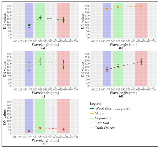
Figure 3.
Analysis considering the raw digital number (DN) average values obtained for 500 ground truth points for each class: (a) Bermudagrass; (b) straw; (c) sugarcane; (d) bare soil; (e) dark objects. The RGB band wavelengths, considering sensor specifications, are highlighted in the respective colored squares. The error bars represent one standard deviation.
3.2. Error Matrix and Validation Metrics
Table 2 shows the OA for the validation dataset and the eight experiments. The OA with no texture features on the dataset was 83.00%, while the best result, an OA of 92.54%, was achieved by using textures with a 15 × 15 window size. The producer (PA) and user (UA) accuracies for each of the five classes in the eight experiments realized are shown in Figure 4. The error matrix (in a pixel count) for the experiment without texture and for the experiment where the best OA was achieved (with textures generated by a 15 × 15 window) are presented in Table 3. Complementary error matrices are presented as Supplementary Materials.
Table 2.
Overall accuracy (OA) (%) for the eight experiments realized.
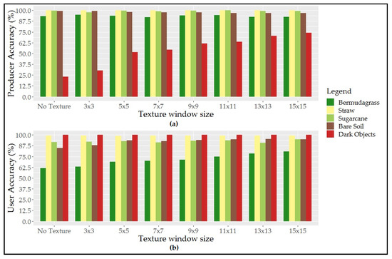
Figure 4.
(a) Producer accuracy (PA) and (b) user accuracy (UA) for each class in the eight experiments realized.
Table 3.
Matrices for experiment 1, without texture, and for experiment 8, which used texture with a 15 × 15 window.
3.3. Classified Images
Figure 5 presents the classified images from experiments 1 and 8, from which theerror matricesare presented in Table 3. Three sample regions were selected and zoomed in on for a better visualization of the results.
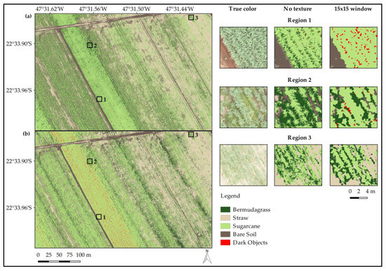
Figure 5.
Images considering (a) the experiment without texture and (b) the experiment that used texture calculated from a 15 × 15 window. Three different regions were selected and zoomed in on for better visualization of the original RGB composition and the classification results for images (a) and (b).
4. Discussion
The first analysis was based onthe spectral characteristics presented in Figure 3. The spectral response of the classes of Bermudagrass and sugarcane were similar and presented characteristics of targets that contained green vegetation [33]. These characteristics included lower digital number (DN) values for the blue band when compared to the respective values of green and red bands. This could be justified by the absorption of electromagnetic energy by leaf components such as chlorophyll A and B, carotenoids, and xanthophylls [33,34]. For the green band, this absorption was reduced, resulting in more electromagnetic energy reflected and thus higher values of DN. For the red band, the absorption of electromagnetic energy increased once again, specially for some leaf components such as chlorophyll A and B, resulting in higher DN values when compared to the blue band, but usually lower DN values than the green band [33,34].
The sugarcane and Bermudagrass classes also presented higher standard deviation values when compared to other classes. The explanation for such variance in pixel DN values is the multiple scattering of electromagnetic energy on multilayer canopies [33]. When an electromagnetic energy bean reaches the first level of a canopy (e.g., a sugarcane leaf on the top of the canopy), the energy can be transmitted, absorbed, or reflected. The transmitted energy hits targets on a second level (under the first leaf), such asa soil patch or another sugarcane leaf. On this second level, the remaining electromagnetic energy is partially reflected back and hits the bottom of the first sugarcane leaf, and is absorbed, reflected back, or transmitted to the atmosphere. This process repeats for targets on other levels. Different targets on the second level caused differences in the first-level DN values and hence a greater standard deviation for the Bermudagrass and sugarcane classes when compared to classes that had no canopy, such as bare soil and straw [33,34,35,36].
The classes of straw and bare soil had spectral responses different from the two previous classes. The class of straw contained parts of vegetation (mostly leaves) derived from previous sugarcane plantations. However, the leaf components related to absorption of the electromagnetic energy, such aschlorophyll A and B, carotenoids, and xanthophylls, were dead and led to almost no absorption from this kind of land cover [33]. This led to the highest DN values obtained in this study. On the other hand, the bare soil class presented increasing DN values for greater wavelength values in the visible region [400–700 nm], characterizing an exposed soil class [37,38]. As mentioned in Table 1, some samples of the bare soil class were not well drained, resulting in high soil moisture, which contributed to a reduction in the DN values when compared to samples that were dry [33,37]. This also contributed to a higher standard deviation in the bare soil class when compared to more homogeneous classes, such as straw or dark objects. The dark objects were shadows generated by overlapping sugarcane plants, and they had low DN values for all bands.
After the spectral analysis, the overall accuracy (OA) values presented in Table 2 were analyzed. Experiment 1, which used only the RGB bands and the GRVI, had an OA of 83.00%. In all experiments with texture features, the OA value was always superior in comparison to datasets with no texture features. For greater window sizes, higher values of OA were observed, reaching 92.54% for the best case scenario (experiment 8 with textures from the 15 × 15 window). The explanation for this relies on the “edge effect”, where the window size used for texture calculation overlaps the border between distinct objects in the image (Figure 6). A window size that is partly over one natural texture and partly over another (along with the edge between them) will, very likely, be less ordered than a window entirely inside a patch of similar texture [20].
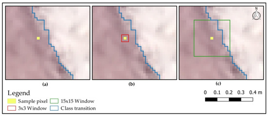
Figure 6.
Explanation of the “edge effect”: (a) A sample pixel on an RGB composition and a hypothetical class transition between bare soil (brown pixels) and straw (light beige pixels) in the study site; (b) a 3 × 3 window used for texture calculation provides an example where the “edge effect” does not occur, since the window is entirely located in one class; (c) a 15 × 15 window used for texture calculation capturing the texture transition between these two classes and representing the “edge effect”.
Some textures, such as contrast, dissimilarity, entropy, and homogeneity, are highly affected by the “edge effect” and can be more useful in discriminating between patches that have two different textures. On the other hand, textures such as mean and variance are more useful in describing the interior of objects, where edges do not occur. Considering that our dataset had more features that could describe the occurrence of two different textures in a window, which translated into two different classes for this application, a better OA was expected for greater window sizes.
Neither of the previously revised works stated how texture window size affected OA, and a comparison of these applications wasrealizedby analyzing the best OA obtained. Considering weed detection applications in other crops, the OA obtained for Bermudagrass detection in sugarcane crops was better than those obtained foreggplants (75.4%), maize (79.0%), and vineyards (83.3%) [15,16,18]. Furthermore, an OA of 92.5% was close to the best performances found in the literature: Weed detection in spinach (96.9%), sunflowers (95.5%), and beans (94.8%) [15,17]. A review of these studies is listed in Table 4.
Table 4.
Several weed detection applications considering factors such as overall accuracy (OA) and the respective classifier and types of features used.
The high OA values obtained by applications in spinach and beans may have been related to the classifier (convolutional neural networks (CNNs)) used [17,24]. CNNs are adeep learning area approach and have been successfully applied in several remote sensing applications [39,40]. Classifications using CNNs in aerial images is usually performed pixel by pixel, and the algorithm is capable of learning representations of the data on multiple levels of abstraction [24,41]. These representations start as simple image features, such as borders, edges, or colors, but evolve into image patterns and pattern associations [24], providing a powerful tool for applications involving weed detection [17].
When comparing our results to other sugarcane applications that did not use texture features, the detection of Bermudagrass was more effective than the detection of sourgrass (77.9%) and tridax daisy (85.5%) [1]. The classification of peppergrass, the shoo-fly plant, and signalgrass, described by Reference [25], obtained an OA of 91.6%. However, the authors did not perform any type of validation and it is possible that this value was overfitted to the dataset used to train the neural network used for classification. A similar OA (92.5%) was obtained by Reference [27] for the classification of sugarcane plants affected by the mosaic virus. However, the UAV image used by Reference [27] had 13 bands and a greater potential to discriminate classes using only spectral information. It is clear that the use of texture in UAV images is capable of improving weed detection in sugarcane crops, but further discussions may be developed to analyze the outputs of the error matrix and the user (UA) and producer (PA) accuracies (Table 3 and Figure 4, respectively).
For the experiment that did not use texture features, the error matrix showed misclassification errors between the classes of dark objects with both Bermudagrass and bare soil. These errors could be translated into low values of PA for the dark objects (23.0%) and UA for Bermudagrass (61.4%) and for bare soil (85.1%). These classes, especially Bermudagrass and dark objects, had a similar spectral behavior, and the use of features that only represented spectral reflectance was not enough to discriminate between them. A similar problem was found by Reference [13] when trying to discriminate between different weed types using only spectral information. On the other hand, when texture features were used, the PA of dark objectsimproved to 74.0% and the UA of the Bermudagrass and bare soil to 80.9% and 94.7%, respectively. The explanation of this relies on the fact that the greater window sizes could detect two different textures between classes, as explained by the “edge effect”. This difference may be visually observed in region 1, highlighted in Figure 5, where the classification without texture barely detected points of dark objects, represented in small red regions.
Another important point is that a few pixels of Bermudagrass were incorrectly classified as sugarcane plants. This was a minor source of error between these two classes but is important to discuss since it represents the omission of Bermudagrass spots in the classification. These errors were more representative for other weeds such as sourgrass and the shoo-fly plant [1,25] and may lead to incorrect assumptions about the level of infestation and also the correct time to apply herbicides to the plantation.
As mentioned in Section 2.1., the study site represented a very heterogeneous plantation, with different sizes of sugarcane plants. Regions 2 and 3, from Figure 5, represented this heterogeneity in two areas that contained sugarcane plants in different growth stages and were both affected by Bermudagrass infestation. For both cases, the use of UAV images and texture features could detect weeds between and within crop rows. Considering that Bermudagrass has more potential to harm sugarcane plants in early growth stages, the combination of UAV and texture features was also suitable for this period.
From an analysis of Figure 5b, the total mapping area, considering the removal of roads, was 11.36 ha. Sugarcane plants represented 47.8% of the area (5.43 ha), while Bermudagrass infestation represented 11.0% of the area (1.25 ha). The other classes (bare soil, straw, and dark objects) were represented by the remaining 41.2% of the area (4.68 ha). The area distribution for each class reflected the highly heterogeneous study site. Considering an average sugarcane productivity of 86.6 tons*ha−1 for the Iracemápolis municipality, the study site can produce up to 470 tons of sugarcane, 55 tons of sugar products, or 4.700 L of ethanol [2,3].
The yield losses caused by Bermudagrass are hardly assessed with precision, since they are heavily dependent on sugarcane variety, ground straw management, and the chemical control used [10,11]. Considering that losses caused by Bermudagrass on sugarcane plantations are estimated between 6% and 14% of yield production [4], the losses from this application ranged from 28.2 to 65.8 tons of sugarcane, or an average loss of up to 12.1 tons*ha−1.
5. Conclusions
Sugarcane has an important role in the Brazilian economy, representing an annual budget of 12.2 billion dollars. Maintaining a high yield production is crucial, and thus monitoring factors such assoil type, availability of water, and weed control in sugarcane plantations is an essential task. One way to provide reliable results for weed occurrence is through UAV images, which can identify targets from above and reduce time and field campaigns to obtain this information. Several weed mapping applications have combined vegetation indices and texture features to achieve better classification results. However, this combination had not yet been tested on sugarcane plantations.
In our study, texture features from the gray-level co-occurrence matrix improved the classification accuracy of Bermudagrass in sugarcane crops using the random forest classifier. The overall accuracy for the experiment using only RGB band values and a vegetation index was 83.0%. When textures were added into this dataset, the overall accuracy increased up to 92.5%, a better result compared to other sugarcane weed detection studies. The producer accuracy of Bermudagrass was higher when larger window sizes were used for texture calculation, due to the capability of representing two different textures in that window. Our results indicate that UAV images and texture features are a good combination to provide reliable detection of Bermudagrass on sugarcane crops in Brazil.
Supplementary Materials
The following are available online at https://www.mdpi.com/2504-446X/3/2/36/s1, Table S1: Error matrices for the experiments 1, without texture, and for experiments 2 to 8 (texture with windows ranging from 3 × 3 to 15 × 15).
Author Contributions
Conceptualization, C.D.G.-N.; data curation, C.D.G.-N., I.D.S., A.K.N., T.S.K., M.C.A.P., and L.E.O.e.C.d.A.; formal analysis, C.D.G.-N., I.D.S., A.K.N. and V.H.R.P.; investigation, C.D.G.-N., V.H.R.P., and M.C.A.P.; methodology, C.D.G.-N. and I.D.S.; resources, I.D.S. and L.E.O.e.C.d.A.; software, C.D.G.-N. and T.S.K.; validation, C.D.G.-N.; writing—original draft, C.D.G.-N., I.D.S., A.K.N., and V.H.R.P.; writing—review and editing, I.D.S., T.S.K., M.C.A.P. and L.E.O.e.C.d.A.
Funding
This research received no external funding.
Acknowledgments
Special thanks to the personnel of Iracemafarm, including Fabiano Cesar Coelho, for collaborating on field campaigns for image acquisition and weed identification.
Conflicts of Interest
The authors declare no conflict of interest.
References
- Yano, I.H.; Alves, J.R.; Santiago, W.E.; Mederos, B.J. Identification of weeds in sugarcane fields through images taken by UAV and random forest classifier. IFAC-PapersOnLine 2016, 49, 415–420. [Google Scholar] [CrossRef]
- Brazilian Union of Sugarcane Industry—UNICA. Available online: http://www.unicadata.com.br (accessed on 6 January 2019).
- Brazilian Ministry of Agriculture Livestock and Food Supply—MAPA. Available online: http://indicadores.agriculta.gov.br/index.htm (accessed on 7 January 2019).
- Huang, Y.K.; Li, W.F.; Zhang, R.Y.; Wang, X.Y. Color Illustration of Diagnosis and Control for Modern Sugarcane Diseases, Pests, and Weeds, 1st ed.; Springer: Singapore, 2018; 420p. [Google Scholar] [CrossRef]
- Aranda, M.A.; Freitas-Astúa, J. Ecology and diversity of plant viruses, and epidemiology of plant virus-induced diseases. Ann. Appl. Biol. 2017, 171, 1–4. [Google Scholar] [CrossRef]
- Bellé, C.; Kaspary, T.E.; Kuhn, P.R.; Schmitt, J.; Lima-Medina, I. Reproduction of Pratylenchus zeae on Weeds. Planta Daninha 2017, 35, 1–8. [Google Scholar] [CrossRef][Green Version]
- Samson, P.; Sallam, N.; Chandler, K. Pests of Australian Sugarcane: Field Guide, 1st ed.; BSES Limited: Indooroopilly, Australia, 2013; 97p. [Google Scholar]
- Johansen, K.; Sallam, N.; Robson, A.; Samson, P.; Chandler, K.; Derby, L.; Eaton, A.; Jennings, J. Using GeoEye-1 Imagery for Multi-Temporal Object-Based Detection of Canegrub Damage in Sugarcane Fields in Queensland, Australia. GISci. Remote Sens. 2018, 55, 285–305. [Google Scholar] [CrossRef]
- Fontenot, D.P.; Griffin, J.L.; Bauerle, M.J. Bermudagrass (Cynodondactylon) competition with sugarcane at planting. J. Am. Soc. Sugar Cane Technol. 2016, 36, 19–30. [Google Scholar]
- Paula, R.J.D.; Esposti, C.D.; Toffoli, C.R.D.; Ferreira, P.S. Weed interference in the initial growth of meristem grown sugarcane plantlets. RevistaBrasileira de Engenharia Agrícola e Ambiental 2018, 22, 634–639. [Google Scholar] [CrossRef]
- Concenco, G.; Leme Filho, J.R.A.; Silva, C.J.; Marques, R.F.; Silva, L.B.X.; Correia, I.V.T. Weed Occurrence in Sugarcane as Function of Variety and Ground Straw Management. Planta Daninha 2016, 34, 219–228. [Google Scholar] [CrossRef]
- Fernández-Quintanilla, C.; Peña, J.M.; Andújar, D.; Dorado, J.; Ribeiro, A.; López-Granados, F. Is the current state of the art of weed monitoring suitable for site-specific weed management in arable crops? Weed Res. 2018, 58, 259–272. [Google Scholar] [CrossRef]
- Caturegli, L.; Lulli, F.; Foschi, L.; Guglielminetti, L.; Bonari, E.; Volterrani, M. Turfgrass spectral reflectance: Simulating satellite monitoring of spectral signatures of main C3 and C4 species. Precis. Agric. 2015, 16, 297–310. [Google Scholar] [CrossRef]
- Motohka, T.; Nasahara, K.; Oguma, H.; Tsuchida, S. Applicability of green-red vegetation index for remote sensing of vegetation phenology. Remote Sens. 2010, 2, 2369–2387. [Google Scholar] [CrossRef]
- Pérez-Ortiz, M.; Penã, J.M.; Gutiérrez, P.A.; Torres-Sánches, J.; Hervás-Martinez, C.; López-Granados, F. Selecting patterns and features for between-and within-crop-row weed mapping using UAV-imagery. Expert Syst. Appl. 2016, 47, 85–94. [Google Scholar] [CrossRef]
- David, L.C.G.; Ballado, A.H. Vegetation indices and textures in object-based weed detection from UAV imagery. In Proceedings of the 6th IEEE International Conference on Control System, Computing and Engineering, Penang, Malaysia, 25–27 November 2016; pp. 273–278. [Google Scholar] [CrossRef]
- Bah, M.; Hafiane, A.; Canals, R. Deep Learning with Unsupervised Data Labeling for Weed Detection in Line Crops in UAV Images. Remote Sens. 2018, 10, 1690. [Google Scholar] [CrossRef]
- Castro, A.I.; Penã, J.M.; Torres-Sánches, J.; Jiménez-Brenes, F.; López-Granados, F. Mapping Cynodondactylon in vineyards using UAV images for site-specific weed control. Adv. Anim.Biosci. 2017, 8, 267–271. [Google Scholar] [CrossRef]
- Haralick, R.M. Statistical and structural approaches to texture. Proc. IEEE 1979, 67, 786–804. [Google Scholar] [CrossRef]
- Hall-Beyer, M. Practical guidelines for choosing GLCM textures to use in landscape classification tasks over a range of moderate spatial scales. Int. J. Remote Sens. 2017, 38, 1312–1338. [Google Scholar] [CrossRef]
- Cortes, C.; Vapnik, V. Support-vector networks. Mach. Learn. 1995, 20, 273–297. [Google Scholar] [CrossRef]
- Hall, M.; Frank, E.; Holmes, G.; Pfahringer, B.; Reutemann, P.; Witten, I.H. The WEKA data mining software: An update. ACM SIGKDD Explor.Newslett. 2009, 11, 10–18. [Google Scholar] [CrossRef]
- Breiman, L. Random forests. Mach. Learn. 2001, 45, 5–32. [Google Scholar] [CrossRef]
- Lecun, Y.; Bengio, Y.; Hinton, G. Deep learning. Nature 2015, 521, 436–444. [Google Scholar] [CrossRef]
- Yano, I.H.; Santiago, W.E.; Alves, J.R.; Mota, L.T.M.; Teruel, B. Choosing classifier for weed identification in sugarcane fields through images taken by UAV. Bulg. J. Agric. Sci. 2017, 23, 491–497. [Google Scholar]
- Dony, R.D.; Haykin, S. Neural network approaches to image compression. Proc. IEEE 1995, 83, 288–303. [Google Scholar] [CrossRef]
- Moriya, E.A.S.; Imai, N.N.; Tommaselli, A.M.G.; Miyoshi, G.T. Mapping mosaic virus in sugarcane based on hyperspectral images. IEEE J. Sel. Top. Appl. Earth Obs. Remote Sens. 2017, 10, 740–748. [Google Scholar] [CrossRef]
- Du, Y.; Chang, C.I.; Ren, H.; Chang, C.C.; Jensen, J.O.; D’Amico, F.M. New hyperspectral discrimination measure for spectral characterization. Opt. Eng. 2004, 43, 1777–1787. [Google Scholar] [CrossRef]
- Belgiu, M.; Drăguţ, L. Random forest in remote sensing: A review of applications and future directions. ISPRS J. Photogramm. Remote Sens. 2016, 114, 24–31. [Google Scholar] [CrossRef]
- Nebiker, S.; Annen, A.; Scherrer, M.; Oesch, D. A light-weight multispectral sensor for micro UAV—Opportunities for very high resolution airborne remote sensing. In International Archives of the Photogrammetry, Remote Sensing and Spatial Information Sciences; ISPRS: Beijing, China, 2008; Volume 37-B1, pp. 1193–1199. [Google Scholar]
- Candiago, S.; Remondino, F.; Giglio, M.; Dubbini, M.; Gattelli, M. Evaluating multispectral images and vegetation indices for precision farming applications from UAV images. Remote Sens. 2015, 7, 4026–4047. [Google Scholar] [CrossRef]
- Sony STARVIS®/Exmor®—Camera Sensor Technology Overview. Available online: https://www.ptgrey.com/exmor-r-starvis (accessed on 12 February 2019).
- Ponzoni, F.J.; Shimabukuro, Y.E.; Kuplich, T.M. Sensoriamento Remoto No Estudo da Vegetação, 2nd ed.; Oficina de Textos: São José dos Campos, Brazil, 2012; 176p. [Google Scholar]
- Formaggio, A.R.; Sanches, I.D. Sensoriamento Remoto em Agricultura, 1st ed.; Oficina de Textos: São José dos Campos, Brazil, 2017; 288p. [Google Scholar]
- Pereira, R.M.; Casaroli, D.; Vellame, L.M.; Alves Júnior, J.; Evangelista, A.W.P. Sugarcane leaf area estimate obtained from the corrected Normalized Difference Vegetation Index (NDVI). Pesqui. Agropecu. Trop. 2016, 46, 140–148. [Google Scholar] [CrossRef]
- Montandon, L.M.; Small, E.E. The impact of soil reflectance on the quantification of the green vegetation fraction from NDVI. Remote Sens. Environ. 2008, 112, 1835–1845. [Google Scholar] [CrossRef]
- Formaggio, A.R.; Epiphanio, J.C.N.; Valeriano, M.M.; Oliveira, J.B. Comportamento espectral (450-2.450 nm) de solos tropicais de São Paulo. Revista Brasileira de Ciência do Solo 1996, 20, 467–474. [Google Scholar]
- Demattê, J.A.M.; Silva, M.L.S.; Rocha, G.C.; Carvalho, L.A.; Formaggio, A.R.; Firme, L.P. Variações espectrais em solos submetidos à aplicação de torta de filtro. Revista Brasileira de Ciência do Solo 2005, 29, 317–326. [Google Scholar] [CrossRef]
- Kussul, N.; Lavreniuk, M.; Skakun, S.; Shelestov, A. Deep learning classification of land cover and crop types using remote sensing data. IEEE Geosc. Remote Sens. Lett. 2017, 14, 778–782. [Google Scholar] [CrossRef]
- Guirado, E.; Tabik, S.; Alcaraz-Segura, D.; Cabello, J.; Herrera, F. Deep-learning versus OBIA for scattered shrub detection with Google earth imagery: Ziziphus Lotus as case study. Remote Sens. 2017, 9, 1220. [Google Scholar] [CrossRef]
- Zhang, C.; Liu, J.; Yu, F.; Wan, S.; Han, Y.; Wang, J.; Wang, G. Segmentation model based on convolutional neural networks for extracting vegetation from Gaofen-2images. J. Appl. Remote Sens. 2018, 12, 042804. [Google Scholar] [CrossRef]


© 2019 by the authors. Licensee MDPI, Basel, Switzerland. This article is an open access article distributed under the terms and conditions of the Creative Commons Attribution (CC BY) license (http://creativecommons.org/licenses/by/4.0/).