Suggestions to Limit Geometric Distortions in the Reconstruction of Linear Coastal Landforms by SfM Photogrammetry with PhotoScan® and MicMac® for UAV Surveys with Restricted GCPs Pattern

 ,
,
Abstract
1. Introduction
2. Photogrammetric Processing Chain
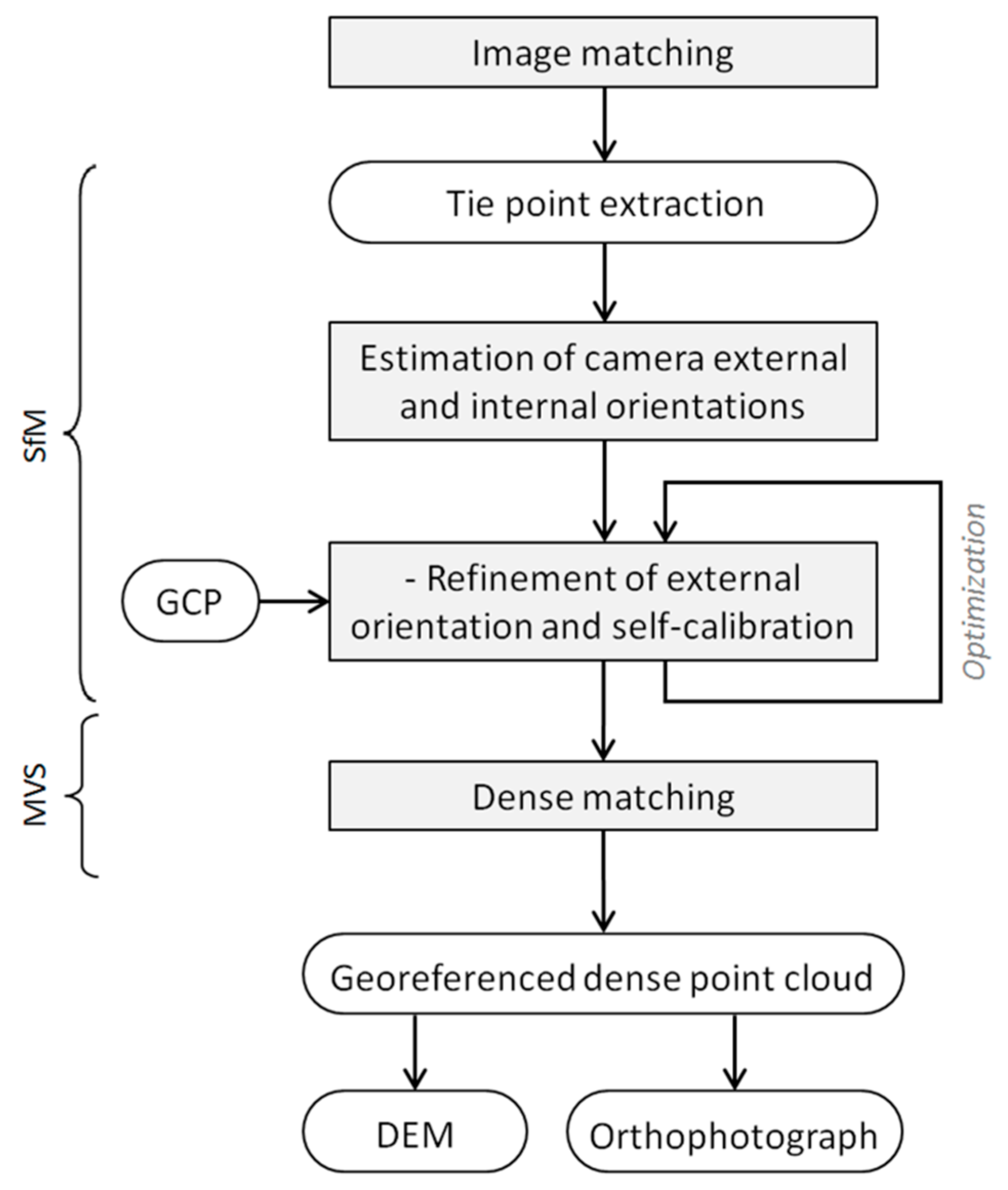
2.1. Principle and Outline of the Photogrammetric Workflow
2.2. PhotoScan Overview
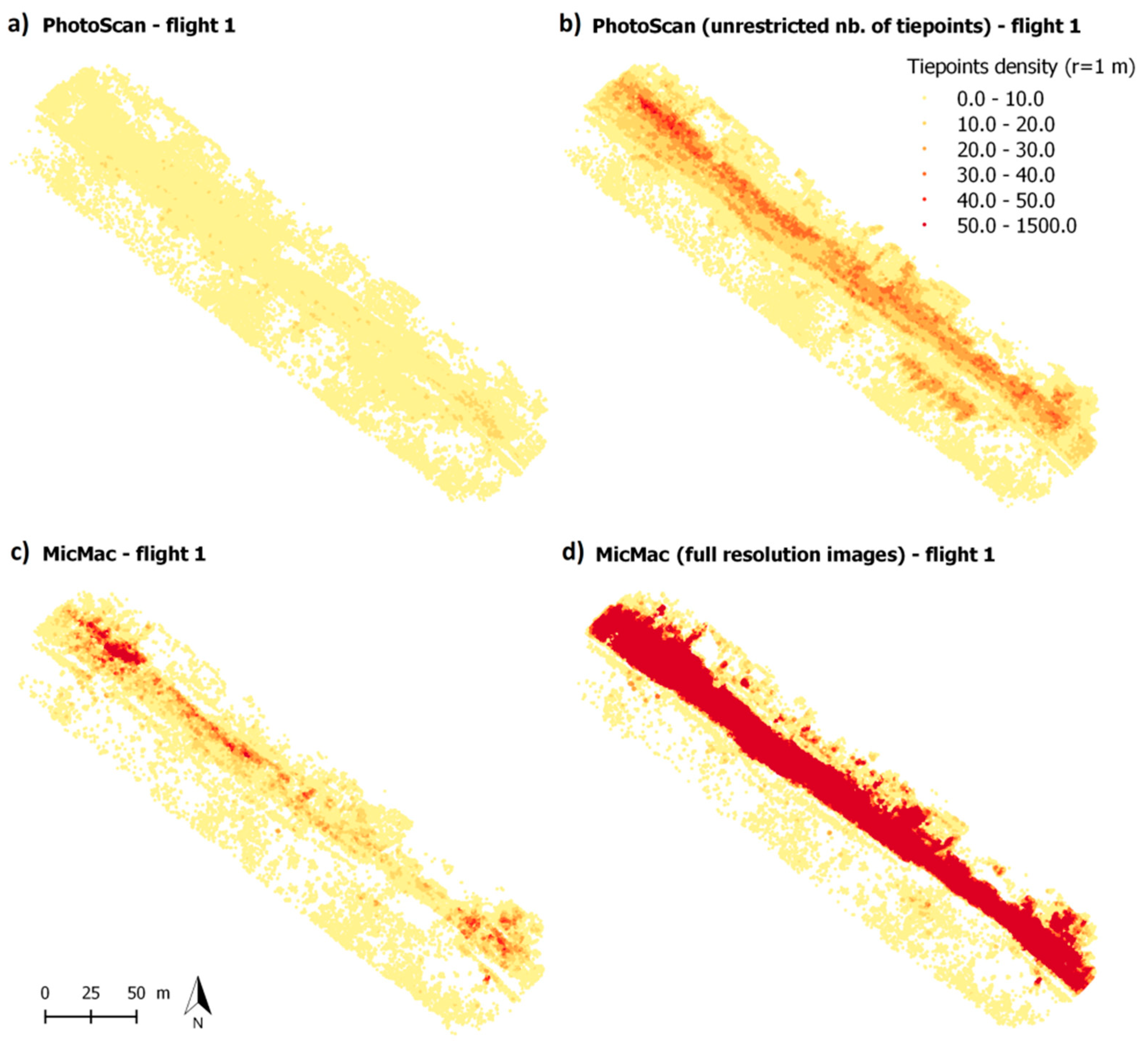
- Image orientation by bundle adjustment. Homologous keypoints are detected and matched on overlapping photographs so as to compute the external camera parameters for each picture. The “High” accuracy parameter is selected (the software works with original size photos) to obtain a more accurate estimation of camera exterior orientation. The number of tie points for every image can be limited to optimize performance. The default value of this parameter (4000) is kept. Tie point accuracy depends on the scale at which they were detected. Camera calibration parameters are refined, including GCPs (ground and image) positions and modelling the distortion of the lens with Brown’s distortion model [30].
- Creation of the dense point cloud by dense image matching using the estimated camera external and internal parameters. The quality of the reconstruction is set to “High” to obtain a more detailed and accurate geometry.
- DEM computation by rasterizing the dense point cloud data on a regular grid.
- Orthophotograph generation based on DEM data.
2.3. MicMac Overview
- Tie point computation: the Pastis tool uses the SIFT++ algorithm [33] for the tie points pairs generation. Here, we used Tapioca, the simplified tool interface, since the features available using Tapioca are sufficient for the purpose of this study. For this step, it is possible to limit processing time by reducing the images size by a factor 2 to 3. By default, the images have been therefore shrunk to a scaling of 0.3.
- External orientation and intrinsic calibration: the Apero tool generates external and internal orientations of the camera. A large panel of distortion models can be used. As mentioned later, two of them are tested in this study. Using GCPs, the images are transformed from relative orientations into an absolute orientation within the local coordinate system using a 3D spatial similarity (“GCP Bascule” tool). Finally the Campari command is used to refine camera orientation by compensation of heterogeneous measures.
- Matching: from the resulting oriented images, MicMac computes 3D models according to a multi-resolution approach, the result obtained at a given resolution being used to predict the next step solution.
- Orthophotograph generation: the tool used to generate orthophotographs is Tawny, the interface of the Porto tool. The individual rectified images that have been previously generated are merged in a global orthophotograph. Optionally, some radiometric equalization can be applied.
2.4. Camera Calibration Models
- f: focal length
- cx, cy: principal point offset
- K1, K2, K3, K4: radial distortion coefficients
- P1, P2, P3, P4: tangential distortion coefficients
- B1, B2: affinity and non-orthogonality (skew) coefficients
3. Conditions of the Field Survey
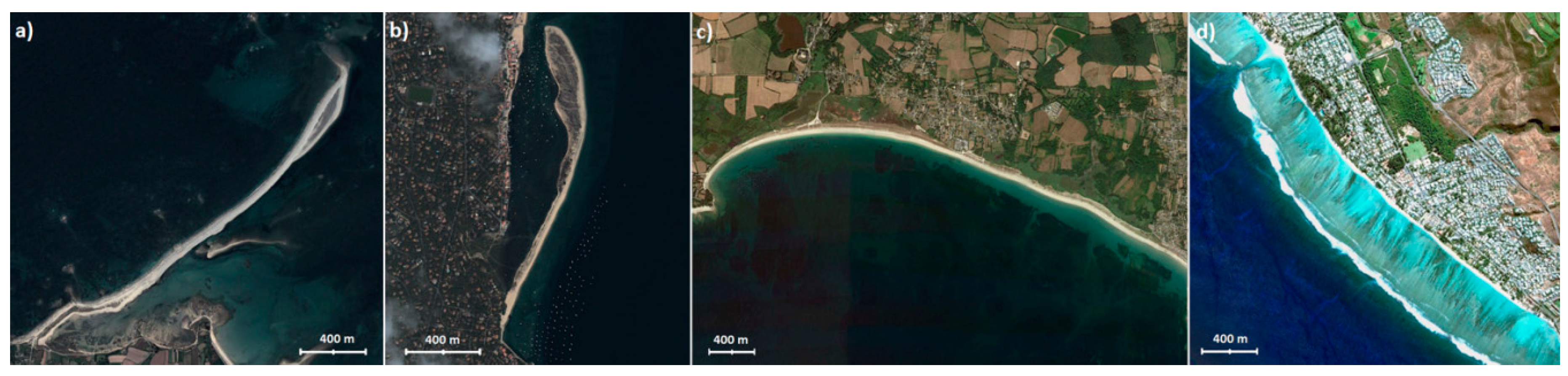
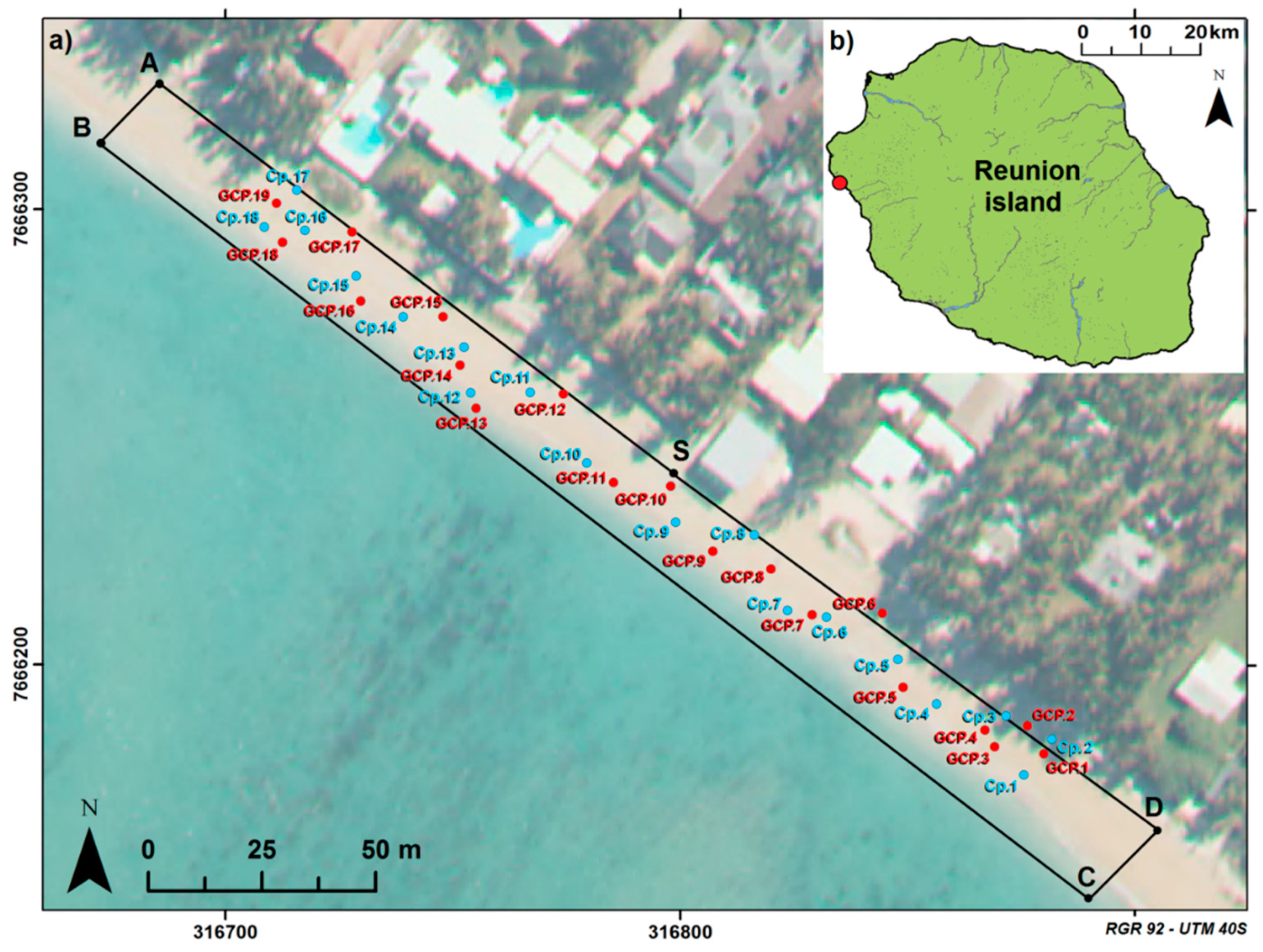
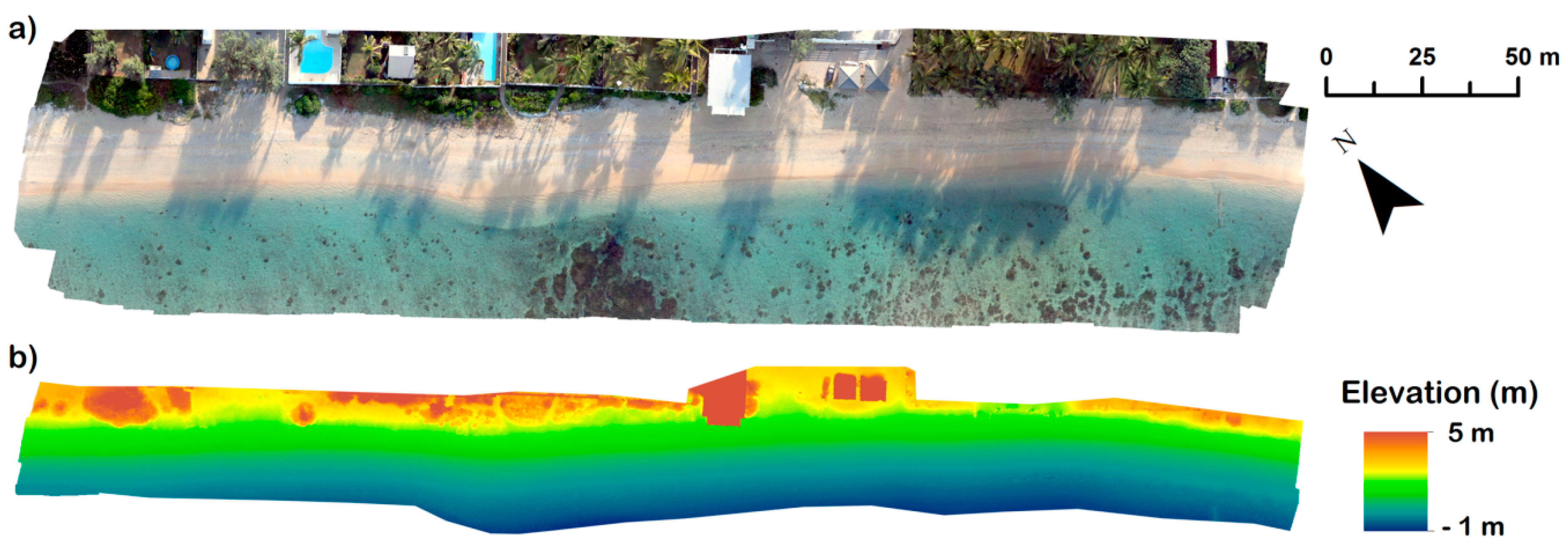
3.1. Study Area
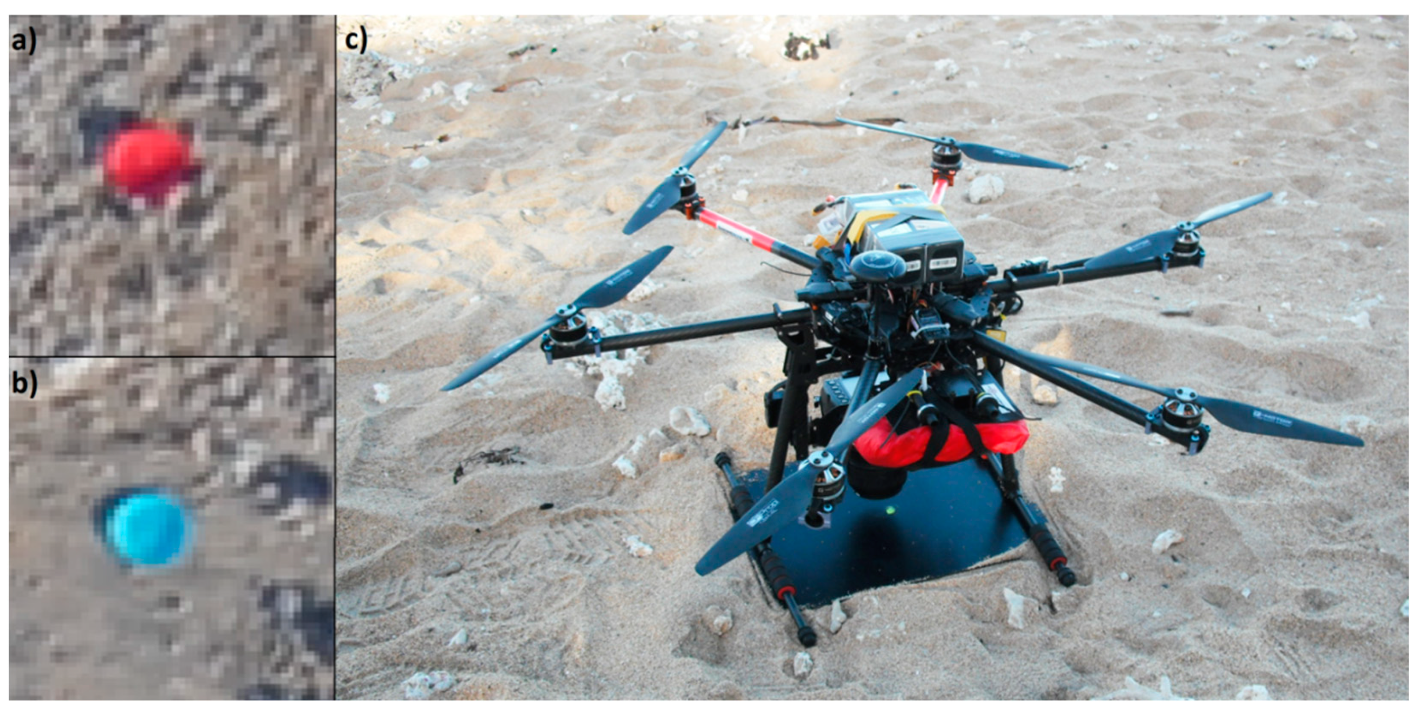
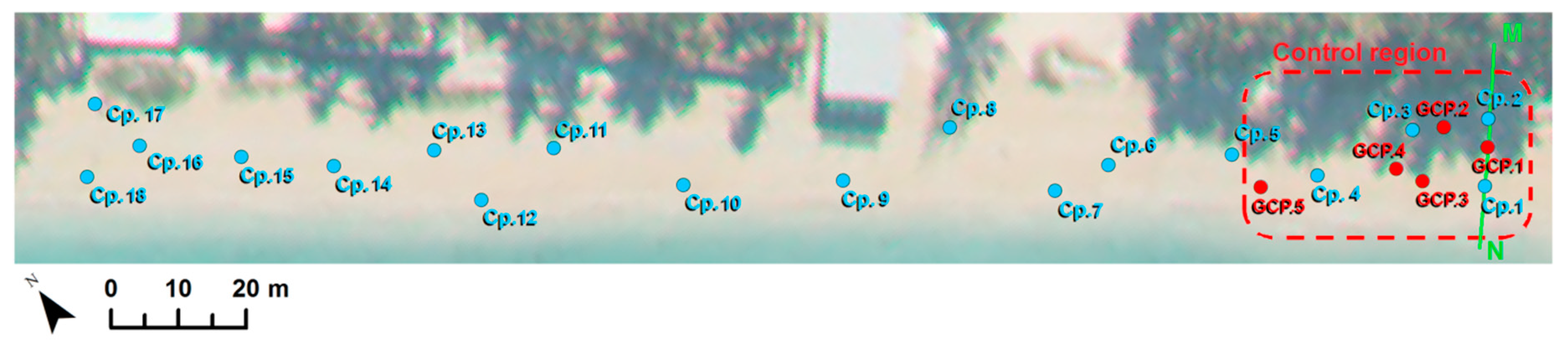
3.2. Ground Control Points and Check Points
3.3. UAV Data Collection
- Flight 1 was performed following a typical flight plan (from S to A, B, C, D and S on Figure 3) with nadir pointing camera and parallel flight lines at a steady altitude of 50 m.
- Flight 2 was performed following the same parallel flight lines at 50 m of altitude with an oblique pointing camera tilted at 40° forward. The inclination has been set to 40° because this angle would be compatible with a survey of the cliff front [36] or of parts of the upper beach situated under the canopy of coastal trees. The two flight lines were carried out in opposite direction. Large viewing angles induce scale variations within each image (from 1.64 cm/pixel to 2.95 cm/pixel). Increasing the tilting angle makes the manual GCPs tagging more difficult.
- Flight 3 was performed following the two parallel flight lines with a nadir-pointing camera but at different altitudes. The altitude was about 40 m from S to A, then 60 m from B to C and finally 40 m from D to S (Figure 3). The disadvantage is that the footprint and the spatial resolution of the photos vary from one flight line to another and therefore the ground coverage is more difficult to plan.
4. Approach for Data Processing
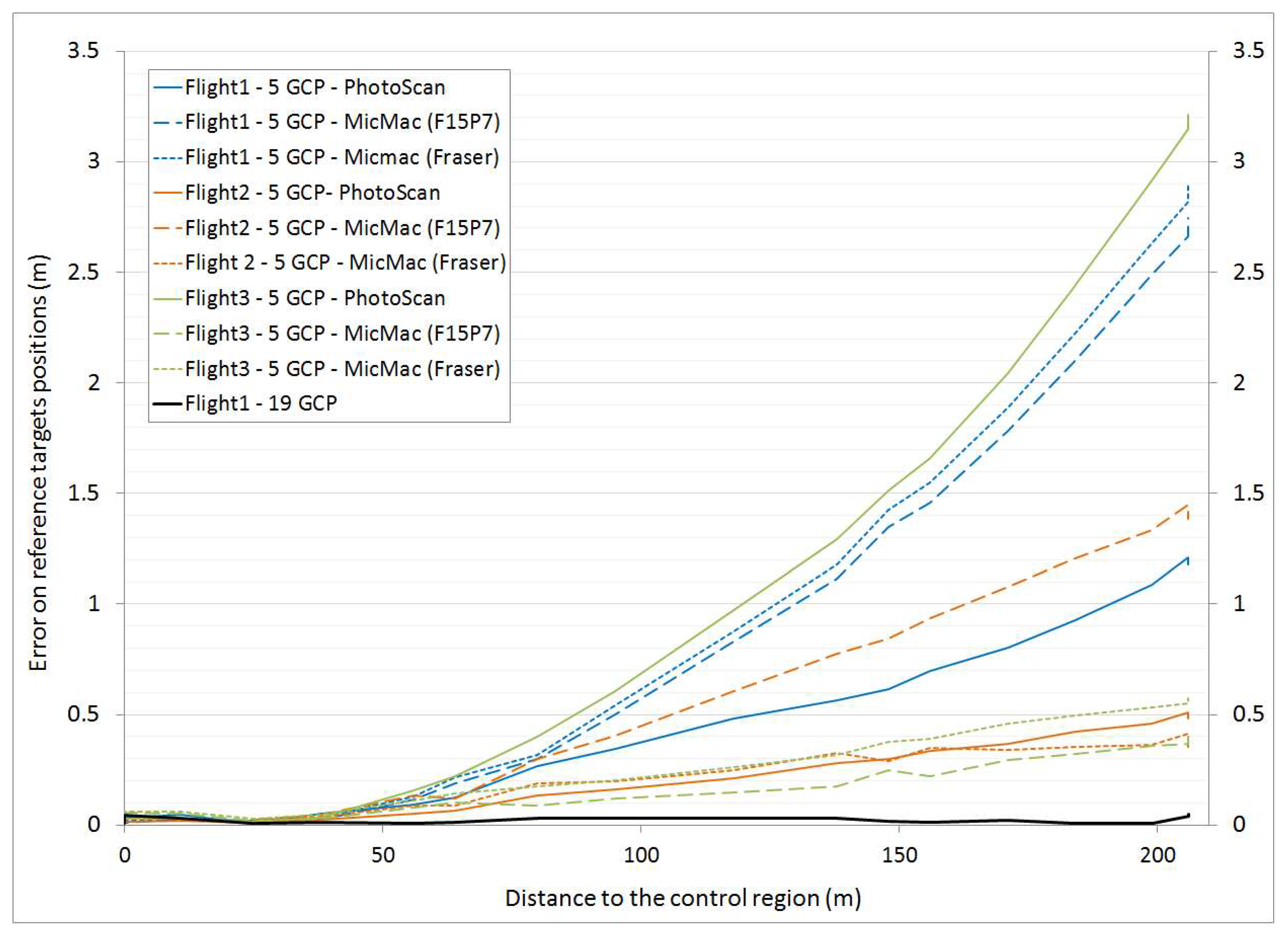
5. Impact of Flight Scenarios on Bowl Effect
6. Discussion
- combining Flight 2 and Flight 3 scenarios, i.e., different altitude of flight with an oblique pointing camera, with perhaps even better results;
- combining Flight 2 or Flight 3 scenario with other optical camera models or processing strategies.
7. Conclusions
Author Contributions
Acknowledgments
Conflicts of Interest
References
- Eltner, A.; Kaiser, A.; Castillo, C.; Rock, G.; Neugirg, F.; Abellán, A. Image-Based Surface Reconstruction in Geomorphometry Merits—Limits and Developments. Earth Surf. Dyn. 2016, 4, 359–389. [Google Scholar] [CrossRef]
- Mancini, F.; Dubbini, M.; Gattelli, M.; Stecchi, F.; Fabbri, S.; Gabbianelli, G. Using Unmanned Aerial Vehicles (UAV) for High-Resolution Reconstruction of Topography: The Structure from Motion Approach on Coastal Environments. Remote Sens. 2013, 5, 6880–6898. [Google Scholar] [CrossRef]
- Javernick, L.; Brasington, J.; Caruso, B. Modeling the Topography of Shallow Braided Rivers Using Structure-from-Motion Photogrammetry. Geomorphology 2014, 213, 166–182. [Google Scholar] [CrossRef]
- Harwin, S.; Lucieer, A. Assessing the Accuracy of Georeferenced Point Clouds Produced via Multi-View Stereopsis from Unmanned Aerial Vehicle (UAV) Imagery. Remote Sens. 2012, 4, 1573–1599. [Google Scholar] [CrossRef]
- Delacourt, C.; Allemand, P.; Jaud, M.; Grandjean, P.; Deschamps, A.; Ammann, J.; Cuq, V.; Suanez, S. DRELIO: An Unmanned Helicopter for Imaging Coastal Areas. J. Coast. Res. 2009, 56, 1489–1493. [Google Scholar]
- Fonstad, M.A.; Dietrich, J.T.; Courville, B.C.; Jensen, J.L.; Carbonneau, P.E. Topographic Structure from Motion: A New Development in Photogrammetric Measurement. Earth Surf. Process. Landf. 2013, 38, 421–430. [Google Scholar] [CrossRef]
- Micheletti, N.; Chandler, J.H.; Lane, S.N. Structure from motion (SFM) photogrammetry. In Geomorphological Techniques; online ed.; Cook, S.J., Clarke, L.E., Nield, J.M., Eds.; British Society for Geomorphology: London, UK, 2015. [Google Scholar]
- Westoby, M.J.; Brasington, J.; Glasser, N.F.; Hambrey, M.J.; Reynolds, J.M. Structure-from-Motion Photogrammetry: A Low-Cost, Effective Tool for Geoscience Applications. Geomorphology 2012, 179, 300–314. [Google Scholar] [CrossRef]
- James, M.R.; Robson, S. Straightforward Reconstruction of 3D Surfaces and Topography with a Camera: Accuracy and Geoscience Application. J. Geophys. Res. Earth Surf. 2012, 117, F3. [Google Scholar] [CrossRef]
- Smith, M.W.; Carrivick, J.L.; Quincey, D.J. Structure from Motion Photogrammetry in Physical Geography. Progr. Phys. Geogr. 2016, 40, 247–275. [Google Scholar] [CrossRef]
- Colomina, I.; Molina, P. Unmanned Aerial Systems for Photogrammetry and Remote Sensing: A Review. ISPRS J. Photogramm. Remote Sens. 2014, 92, 79–97. [Google Scholar] [CrossRef]
- Jaud, M.; Grasso, F.; Le Dantec, N.; Verney, R.; Delacourt, C.; Ammann, J.; Deloffre, J.; Grandjean, P. Potential of UAVs for Monitoring Mudflat Morphodynamics (Application to the Seine Estuary, France). ISPRS Int. J. Geoinf. 2016, 5, 50. [Google Scholar] [CrossRef]
- James, M.R.; Robson, S. Mitigating Systematic Error in Topographic Models Derived from UAV and Ground-Based Image Networks. Earth Surf. Process. Landf. 2014, 39, 1413–1420. [Google Scholar] [CrossRef]
- Rosnell, T.; Honkavaara, E. Point Cloud Generation from Aerial Image Data Acquired by a Quadrocopter Type Micro Unmanned Aerial Vehicle and a Digital Still Camera. Sensors 2012, 12, 453–480. [Google Scholar] [CrossRef] [PubMed]
- Tournadre, V.; Pierrot-Deseilligny, M.; Faure, P.H. UAV Linear Photogrammetry. Int. Arch. Photogramm. Remote Sens. 2015, XL-3/W3, 327–333. [Google Scholar] [CrossRef]
- Wu, C. Critical Configurations for Radial Distortion Self-Calibration. In Proceedings of the 27th IEEE Conference on Computer Vision and Pattern Recognition, Columbus, OH, USA, 24–27 June 2014. [Google Scholar] [CrossRef]
- Tonkin, T.N.; Midgley, N.G. Ground-Control Networks for Image Based Surface Reconstruction: An Investigation of Optimum Survey Designs Using UAV Derived Imagery and Structure-from-Motion Photogrammetry. Remote Sens. 2016, 8, 786. [Google Scholar] [CrossRef]
- James, M.R.; Robson, S.; d’Oleire-Oltmanns, S.; Niethammer, U. Optimising UAV topographic surveys processed with structure-from-motion: Ground control quality, quantity and bundle adjustment. Geomorphology 2017, 280, 51–66. [Google Scholar] [CrossRef]
- Congress, S.S.C.; Puppala, A.J.; Lundberg, C.L. Total system error analysis of UAV-CRP technology for monitoring transportation infrastructure assets. Eng. Geol. 2018, 247, 104–116. [Google Scholar] [CrossRef]
- Molina, P.; Blázquez, M.; Cucci, D.; Colomina, I. First Results of a Tandem Terrestrial-Unmanned Aerial mapKITE System with Kinematic Ground Control Points for Corridor Mapping. Remote Sens. 2017, 9, 60. [Google Scholar] [CrossRef]
- Skarlatos, D.; Vamvakousis, V. Long Corridor survey for high voltage power lines design using UAV. ISPRS Int. Arch. Photogramm. Remote Sens. 2017, XLII-2/W8, 249–255. [Google Scholar] [CrossRef]
- Matikainen, L.; Lehtomäki, M.; Ahokas, E.; Hyyppä, J.; Karjalainen, M.; Jaakkola, A.; Kukko, A.; Heinonen, T. Remote sensing methods for power line corridor surveys. ISPRS J. Photogramm. Remote Sens. 2016, 119, 10–31. [Google Scholar] [CrossRef]
- Dietrich, J.T. Riverscape mapping with helicopter-based Structure-from-Motion photogrammetry. Geomorphology 2016, 252, 144–157. [Google Scholar] [CrossRef]
- Zhou, Y.; Rupnik, E.; Faure, P.-H.; Pierrot-Deseilligny, M. GNSS-Assisted Integrated Sensor Orientation with Sensor Pre-Calibration for Accurate Corridor Mapping. Sensors 2018, 18, 2783. [Google Scholar] [CrossRef] [PubMed]
- Rehak, M.; Skaloud, J. Fixed-wing micro aerial vehicle for accurate corridor mapping. ISPRS Int. Arch. Photogramm. Remote Sens. 2015, II-1/W1, 23–31. [Google Scholar] [CrossRef]
- Grayson, B.; Penna, N.T.; Mills, J.P.; Grant, D.S. GPS precise point positioning for UAV photogrammetry. Available online: https://onlinelibrary.wiley.com/doi/full/10.1111/phor.12259 (accessed on 22 December 2018).
- Jaud, M.; Passot, S.; Le Bivic, R.; Delacourt, C.; Grandjean, P.; Le Dantec, N. Assessing the Accuracy of High Resolution Digital Surface Models Computed by PhotoScan® and MicMac® in Sub-Optimal Survey Conditions. Remote Sens. 2016, 8, 465. [Google Scholar] [CrossRef]
- Lowe, D.G. Distinctive Image Features from Scale-invariant Keypoints. Int. J. Comput. Vis. 2004, 60, 91–110. [Google Scholar] [CrossRef]
- Seitz, S.M.; Curless, B.; Diebel, J.; Scharstein, D.; Szeliski, R. A Comparison and Evaluation of Multi-View Stereo Reconstruction Algorithms. In Proceedings of the IEEE Computer Society Conference on Computer Vision and Pattern Recognition, New York, NY, USA, 17–23 June 2006. [Google Scholar] [CrossRef]
- AgiSoft PhotoScan User Manual, Professional Edition v.1.2. Agisoft LLC. 2016. Available online: http://www.agisoft.com/pdf/photoscan-pro_1_2_en.pdf (accessed on 14 June 2016).
- Pierrot-Deseilligny, M.; Clery, I. APERO, an Open Source Bundle Adjustment Software for Automatic Calibration and Orientation of Set of Images. ISPRS Int. Arch. Photogramm. Remote Sens. 2011, XXXVIII-5/W16, 269–276. [Google Scholar] [CrossRef]
- Pierrot-Deseilligny, M. MicMac, Apero, Pastis and Other Beverages in a Nutshell! 2015. Available online: http://logiciels.ign.fr/IMG/pdf/docmicmac-2.pdf (accessed on 27 July 2016).
- Vedaldi, A. An Open Implementation of the SIFT Detector and Descriptor; UCLA CSD Technical Report 070012; University of California: Los Angeles, CA, USA, 2007. [Google Scholar]
- Remondino, F.; Fraser, C. Digital Camera Calibration Methods: Considerations and Comparisons. ISPRS Int. Arch. Photogramm. Remote Sens. 2006, XXXVI, 266–272. [Google Scholar]
- Fraser, C.S. Digital camera self-calibration. ISPRS J. Photogramm. Remote Sens. 1997, 52, 149–159. [Google Scholar] [CrossRef]
- Letortu, P.; Jaud, M.; Grandjean, P.; Ammann, J.; Costa, S.; Maquaire, O.; Davidson, R.; Le Dantec, N.; Delacourt, C. Examining high-resolution survey methods for monitoring cliff erosion at an operational scale. GISci. Remote Sens. 2018, 55, 457–476. [Google Scholar] [CrossRef]


| Flight 1 | Flight 2 | Flight 3 | ||||
|---|---|---|---|---|---|---|
| “Classical” | Oblique Pointing Camera (40°) | Varying Altitude | ||||
| Number of images | 83 | 73 | 93 | |||
| Flight altitude (m) | 50 m | 50 m | 40 m/60 m | |||
| Image resolution (cm/pix) | 1.68 | 2.12 [1.64; 2.95] | 1.55 [1.33; 1.77] | |||
| Mean image footprint | 53.5 × 35.6 m | 67.5 × 44.9 m | 49.4 × 32.9 m [42.3 × 28.2 m; 56.4 × 37.5 m] | |||
| Mean distance between camera positions | 7.4 m | 7.7 m | 7.0 m | |||
| Coverage area (m2) | 22,100 | 31,700 | 18,200 | |||
Images overlap  |  |  |  | |||
| PhotoScan | MicMac | PhotoScan | MicMac | PhotoScan | MicMac | |
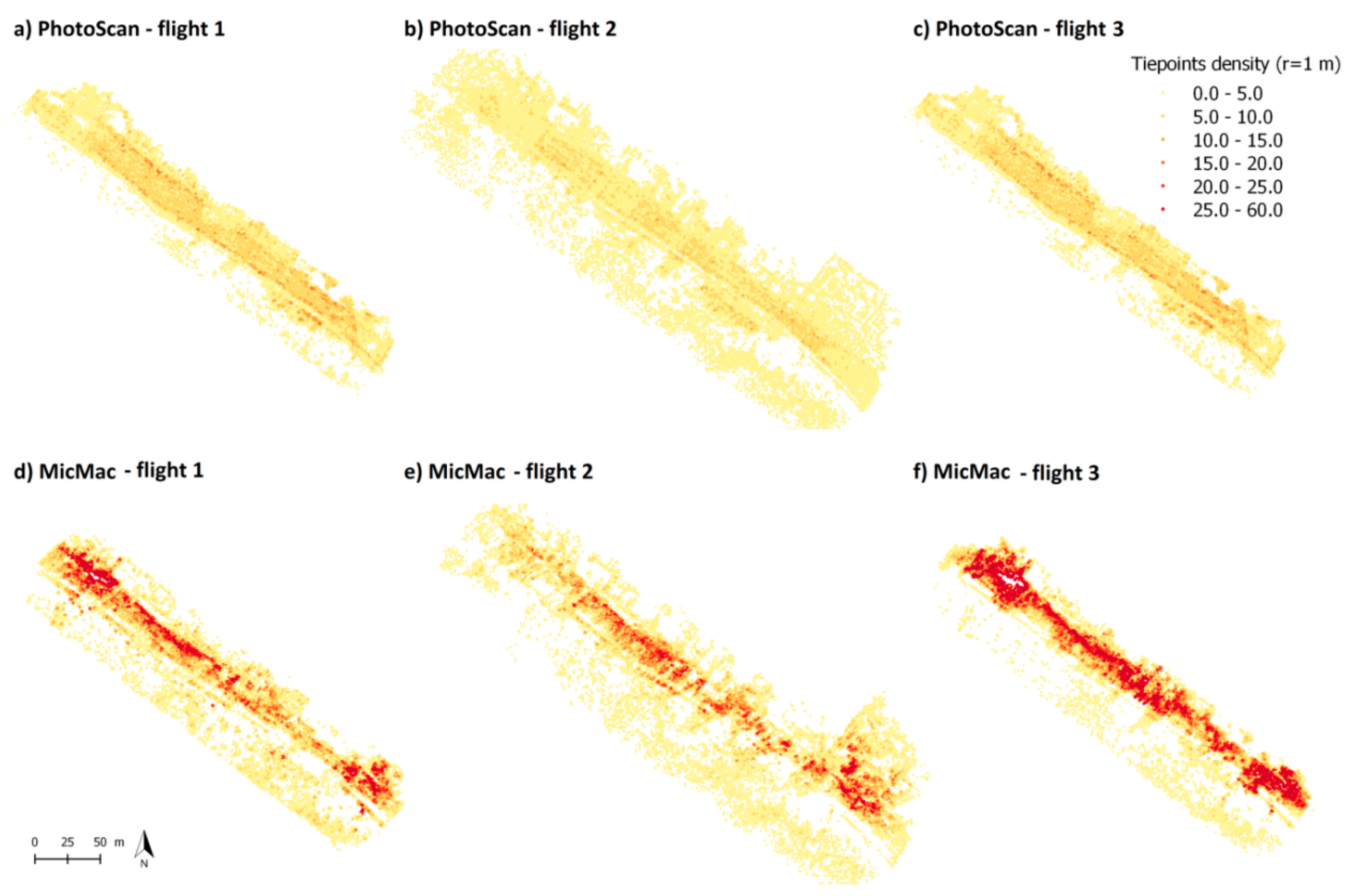
| Number of tie points | 57,781 | 129,478 | 65,382 | 129,977 | 56,376 | 202,890 |
| Average density of tie points in r = 1 m | 5.1 | 22.5 | 3.9 | 12.1 | 6.5 | 36.5 |
| Flight 1 | Flight 2 | Flight 3 | ||||||||||||||||
|---|---|---|---|---|---|---|---|---|---|---|---|---|---|---|---|---|---|---|
| “Classical” | Oblique Pointing Camera (40°) | Varying Altitude | ||||||||||||||||
| With 19 GCPs | ||||||||||||||||||
| PS | MM-F15P7 | PS | MM-F15P7 | PS | MM-F15P7 | |||||||||||||
| XY error 1 (cm) | 1.4 | 1.1 | 1.1 | 2.2 | 1.5 | 1.4 | ||||||||||||
| Z error 1 (cm) | 2.2 | 3.8 | 1.3 | 2.5 | 1.9 | 3.6 | ||||||||||||
| Total error 1 (cm) | 2.6 | 4 | 1.7 | 3.3 | 2.4 | 3.9 | ||||||||||||
| Std. deviation (cm) | 1.4 | 2.1 | 0.7 | 1.2 | 1.1 | 1.4 | ||||||||||||
| RMS reprojection error (pix) | 0.84 | 0.69 | 0.87 | 0.93 | 0.82 | 0.85 | ||||||||||||
| With 5 GCPs | ||||||||||||||||||
| PS | MM-F15P7 | MM-Fra. | PS | MM-F15P7 | MM-Fra. | PS | MM-F15P7 | MM-Fra. | ||||||||||
| XY error 1 (cm) | 30.0 | 3.5 | 6.4 | 20.1 | 16.6 | 18.5 | 16.2 | 12.0 | 7.8 | |||||||||
| Z error 1 (cm) | 55.6 | 138.7 | 146.7 | 19.2 | 79.7 | 18.0 | 160.9 | 17.7 | 32.1 | |||||||||
| Total error 1 (cm) | 63.2 | 138.8 | 146.8 | 27.9 | 81.4 | 25.9 | 161.8 | 21.4 | 32.9 | |||||||||
| Std. deviation (cm) | 42.8 | 100.4 | 106.0 | 18.2 | 53.3 | 14.4 | 117.1 | 12.9 | 19.6 | |||||||||
| RMS reprojection error (pix) | 0.83 | 0.68 | 0.67 | 0.83 | 0.93 | 0.92 | 0.79 | 0.85 | 0.84 | |||||||||
| PhotoScan Restricted nb. of tie points (<4000) | MicMac Reduced Image Size | PhotoScan Unrestricted nb. of tie points | MicMac Full Resolution Images | |
|---|---|---|---|---|
| Number of tie points | 57,781 | 129,478 | 214,374 | 2,449,061 |
| Mean density of tie points in r = 1 m | 5.1 | 22.5 | 20.0 | 469.2 |
| RMS reprojection error (pix) | 0.83 | 0.68 | 0.55 | 0.26 |
© 2018 by the authors. Licensee MDPI, Basel, Switzerland. This article is an open access article distributed under the terms and conditions of the Creative Commons Attribution (CC BY) license (http://creativecommons.org/licenses/by/4.0/).
Share and Cite
Jaud, M.; Passot, S.; Allemand, P.; Le Dantec, N.; Grandjean, P.; Delacourt, C. Suggestions to Limit Geometric Distortions in the Reconstruction of Linear Coastal Landforms by SfM Photogrammetry with PhotoScan® and MicMac® for UAV Surveys with Restricted GCPs Pattern. Drones 2019, 3, 2. https://doi.org/10.3390/drones3010002
Jaud M, Passot S, Allemand P, Le Dantec N, Grandjean P, Delacourt C. Suggestions to Limit Geometric Distortions in the Reconstruction of Linear Coastal Landforms by SfM Photogrammetry with PhotoScan® and MicMac® for UAV Surveys with Restricted GCPs Pattern. Drones. 2019; 3(1):2. https://doi.org/10.3390/drones3010002
Chicago/Turabian StyleJaud, Marion, Sophie Passot, Pascal Allemand, Nicolas Le Dantec, Philippe Grandjean, and Christophe Delacourt. 2019. "Suggestions to Limit Geometric Distortions in the Reconstruction of Linear Coastal Landforms by SfM Photogrammetry with PhotoScan® and MicMac® for UAV Surveys with Restricted GCPs Pattern" Drones 3, no. 1: 2. https://doi.org/10.3390/drones3010002
APA StyleJaud, M., Passot, S., Allemand, P., Le Dantec, N., Grandjean, P., & Delacourt, C. (2019). Suggestions to Limit Geometric Distortions in the Reconstruction of Linear Coastal Landforms by SfM Photogrammetry with PhotoScan® and MicMac® for UAV Surveys with Restricted GCPs Pattern. Drones, 3(1), 2. https://doi.org/10.3390/drones3010002