Article

Coupled Variable-Mass Flight Dynamics and Active Control of Unmanned Cargo Airships with Transient Hydrodynamic Effects

1
School of Aeronautic Science and Engineering, Beihang University, Beijing 102206, China
2
Linzhou (Ningbo) Technology Co., Ltd., Yuyao 315400, China
3
Institute of Unmanned System, Beihang University, Beijing 100191, China
*
Author to whom correspondence should be addressed.
Drones 2026, 10(9), 704; https://doi.org/10.3390/drones10090704
Submission received: 31 July 2026 / Revised: 4 September 2026 / Accepted: 13 September 2026 / Published: 15 September 2026

Highlights

What are the main findings?
  • A six-degree-of-freedom variable-property airship model couples active seawater ballast, reduced transient hydraulics, and constrained flow allocation.
  • Across the tested 0.70–1.30-times nominal pitch-inertia range, variable-property compensation reduces sensitivity; at 1.30 times nominal inertia, the pitch RMS error is reduced by 31.8%, and sustained settling is achieved 12.9 s earlier than with the frozen-inertia PID.
What are the implications of the main findings?
  • Active seawater ballast can be coordinated as a constrained mass-management and flight-control effector during simulated cargo exchange.
  • The results establish numerical feasibility within the declared nominal, inertia, and actuator-time-constant cases and provide a basis for subsequent hydraulic experiments, hardware-in-the-loop testing, and flight validation.

Abstract

Large unmanned cargo airships may support heavy-lift logistics in regions without runway infrastructure, but payload release produces a rapid buoyancy surplus and changes the vehicle mass properties. This study develops a simulation framework coupling six-degree-of-freedom variable-property flight dynamics, an active seawater ballast system, and constrained ballast-flow allocation. The dynamics are referenced to a fixed body origin and retain the spatial-mass-matrix derivative and declared exchange-momentum wrench. A one-dimensional Method-of-Characteristics (MOC) solution provides a numerical reference for the reduced line-inertance runtime model. Fitting yields L eff = 55.240 m and a 15.3% closure-interval normalized root-mean-square error (NRMSE), providing cross-model verification rather than experimental validation. Under the nominal 1201 s mission, the variable-property-aware case satisfies the predeclared criteria with a final-altitude error of 2.985 m and a steady-climb pitch RMS error of 0.165 . A fair frozen-inertia ablation also passes and produces slightly lower nominal errors (2.806 m and 0.157 ); hence, nominal superiority is not claimed. Across the five-point pitch-inertia sweep (0.70 to 1.30 times nominal), the variable-property-aware controller keeps the steady-climb pitch RMS error within 0.137 0.165 , whereas the frozen-inertia proportional–integral–derivative (PID) controller spans 0.153 0.230 ; at 1.30 times nominal inertia, the variable-property-aware controller reduces pitch RMS error by 31.8% and settles 12.9 s earlier. All 21 independently rerun cases that jointly scale the nominal pump and valve time constants from 1.0 to 3.0 satisfy the declared criteria. In the N = 20 , ± 5 % local parameter-dispersion study, all plotted trajectories remain state-bounded, while the wide altitude spread precludes a uniform tracking or reliability claim. The evidence supports numerical feasibility within the explicitly tested nominal, inertia, and actuator-time-constant cases while requiring configuration-specific trim and controller rematching before extrapolation; it does not constitute a reliability probability or global stability proof.

1. Introduction

Mission-specific logistics increasingly shape the design of unmanned aerial platforms [1,2]. Deep-sea resource access, Arctic routes, and resupply of remote archipelagos remain difficult because ports, runways, and local flight crews may be unavailable [1]. Maritime transport requires suitable port infrastructure and favorable sea states, whereas helicopters have limited range and high operating costs. Large unmanned cargo airships combine long endurance, point-to-point delivery, and low-speed hovering, allowing heavy loads to reach infrastructure-poor locations [3,4]. We consider an unmanned cargo airship that uses closed-loop control for descent, ballast exchange, and attitude recovery during cargo delivery.
Payload exchange from an unmanned cargo airship requires stable low-speed operation without direct onboard piloting. Releasing a heavy payload creates a buoyancy surplus that the flight-control system must manage. Existing buoyancy-management systems use several approaches. Pasternak’s Control of Static Heaviness (COSH) system compresses helium into onboard pressure tanks to reduce static lift and therefore requires dedicated compression, storage, and power systems [5,6]. The Lockheed Martin LMH-1 combines helium buoyancy with hull-generated aerodynamic lift and vectored thrust [7,8,9,10]. Recent cargo-airship programs continue to use composite structures [11], although structural design lies outside the present scope. These architectures address operating conditions that differ from the stationary seawater-ballast compensation problem studied here.
Many existing models approximate ballast transfer as a quasi-static point-mass change. Rapid flow changes can generate hydraulic line-inertance and pipe fluid–structure interaction (FSI) loads that this approximation omits [12,13,14]. We therefore use a one-dimensional Method-of-Characteristics (MOC) solution as a numerical reference and a reduced hydraulic model in the coupled runtime simulation. The present model omits structural response and fatigue.
An active Seawater Ballast System (SBS) draws ballast from the surrounding ocean and provides controllable mass flow during unmanned payload exchange. As Figure 1 shows, synchronized seawater intake and cargo unloading can maintain near-neutral buoyancy during hover. Ballast transfer also makes the airship a variable-mass system: tank filling and drainage change total mass, inertia, and center-of-gravity (CG) location, while the pipe network generates transient hydraulic loads. Autonomous descent and post-unloading recovery therefore require an integrated controller for mission commands, vehicle dynamics, and ballast hydraulics.
We investigate coupled flight-dynamics modeling and closed-loop control for an unmanned cargo airship equipped with an active SBS. The simulated mission comprises low-speed descent, payload release, concurrent seawater compensation, and post-unloading flight recovery. The controller maps trajectory and attitude commands to pump and valve commands. Higher-level route planning, perception, and communication remain outside the present scope. The contributions are as follows:
(1)
We formulate the six-degree-of-freedom dynamics about a fixed body origin and retain the spatial-mass-matrix derivative and declared exchange-momentum wrench. A one-dimensional MOC solution provides the numerical reference for calibrating and assessing the reduced line-inertance runtime model.
(2)
We develop a multi-stage hybrid control strategy with inverse-dynamics-based allocation. The allocator distributes total-flow and pitch-moment targets between the ballast tanks under nonnegative-flow, capacity, remaining-volume, and command-rate constraints. This control architecture regulates descent velocity, altitude, and pitch as the mass properties and CG location change.
(3)
We define traceable protocols for the nominal mission, a fair controller ablation, an actuator-time-constant sweep, and a local parameter-dispersion study. These tests identify the simulated controller envelope, quantify the scope of variable-property compensation, and distinguish actuator-dynamics sensitivity from local plant-parameter sensitivity.
The remainder of the paper is organized as follows. Section 2 establishes the variable-property flight dynamics and hydraulic models. Section 3 presents the multi-stage controller and constrained allocation. Section 4 reports numerical verification, fair-ablation, delay, and uncertainty results. Section 5 states conclusions and limitations.

2. Coupled Mathematical Modeling

Table 1 summarizes the scope of the modeling approaches considered here and introduces the coupled formulation developed in this section.

2.1. Modeling Assumptions and Coordinate Systems

2.1.1. Modeling Assumptions

Assumption 1. The atmosphere follows the implemented standard-atmosphere functions, the helium mass and envelope volume are fixed, and the simplified ballonet model maintains a declared 200 Pa overpressure. Detailed thermal and ballonet dynamics have been treated elsewhere [15,16,17]; solar heating, helium superheat, spatial temperature gradients, and envelope thermoelastic deformation are not modeled here.
Assumption 2. The hull is treated as a rigid body. Ballast water and cargo are represented by lumped masses at declared body-frame locations. Tank free-surface motion and sloshing can introduce additional nonlinear dynamics [18], but sloshing, structural deformation, pipe–structure vibration, and fatigue are outside the present model.
Assumption 3. The flight model is six-degree-of-freedom, whereas the control-performance discussion focuses on longitudinal altitude and pitch. The modeled SBS changes total mass through net seawater flow and produces pitch moment through differential front–rear drainage. Lateral–directional motion is retained in the numerical state but is not presented as a separately validated control channel.

2.1.2. Coordinate Systems

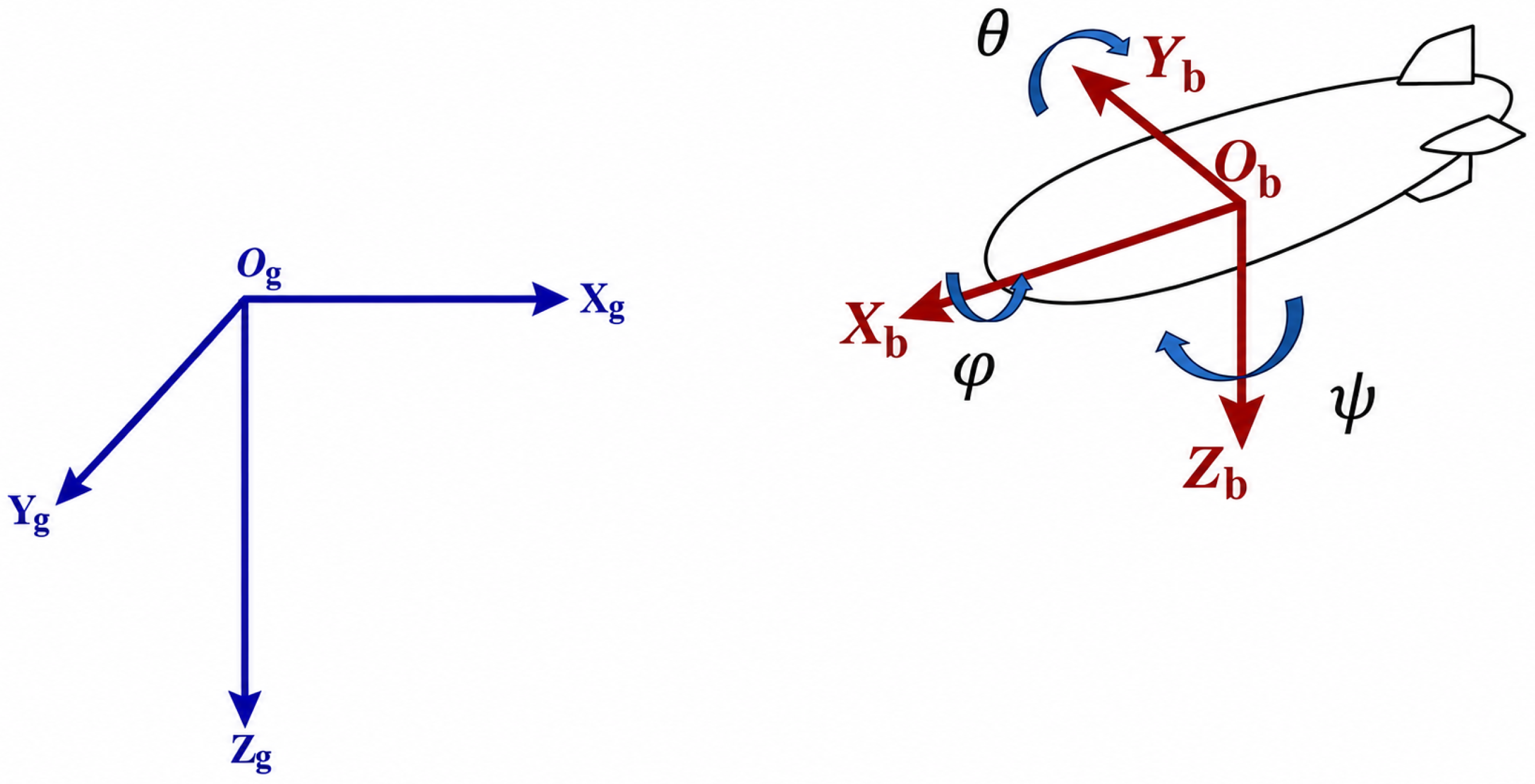
The six-degree-of-freedom variable-property model uses three frames (Figure 2): the earth-fixed navigation frame O g X g Y g Z g , the body-fixed frame O b X b Y b Z b , and a velocity frame defined by the relative air-velocity vector for evaluating aerodynamic coefficients.
The orientation of the body frame relative to the navigation frame is defined by the yaw, pitch, and roll angles ( ψ , θ , φ ) . The transformation from body-frame to navigation-frame components is
X g Y g Z g T = A b g ( ψ , θ , φ ) X b Y b Z b T .
Using the stated yaw–pitch–roll convention,
A b g = R z ( ψ ) R y ( θ ) R x ( φ ) .

2.2. Variable-Mass Six-DOF Flight Dynamics

The flight dynamics are written about the fixed body origin O b , rather than about a center of mass that moves during ballast transfer. Let ν b = [ v b T , ω b T ] T and let S ( r ) x = r × x . The variable-property Newton–Euler balance used here is
M R ( t ) + M A ν ˙ b + C R ( ν b , t ) ν b + M ˙ R ( t ) ν b = W ext + W ex ,
where the rigid-body spatial mass matrix about O b is
M R ( t ) = m ( t ) I 3 m ( t ) S ( r G ( t ) ) m ( t ) S ( r G ( t ) ) I O ( t ) .
Here I O ( t ) is the inertia tensor about the same fixed origin, assembled from the structure, attached cargo, and three lumped ballast masses by the parallel-axis theorem. Thus the lower block of M ˙ R ν b contains not only I ˙ O ω b , but also the derivatives of m S ( r G ) . This avoids treating I ˙ ω b as an isolated correction while the center of mass is moving.
For a port i, m ˙ i > 0 denotes inflow and v rel , i is the fluid velocity relative to the body at the control surface. The resolved exchange-momentum wrench is
W ex = i m ˙ i v rel , i r i × ( m ˙ i v rel , i ) + i F h , i r i × F h , i ,
where the second sum is the optional reduced line-inertance wrench defined in Equation (10). In the implemented drainage convention, m ˙ i < 0 and the outlet-relative velocity points in the positive body-z direction. The force m ˙ i v rel , i and its moment about O b are therefore evaluated together. The pump-inlet turning geometry is not resolved; its relative-velocity contribution is set to zero rather than assigning an unsupported direction, and this limitation is stated explicitly below.

2.3. Aerodynamic Modeling

The low-speed descent and recovery maneuvers require aerodynamic coefficients over the full angle-of-attack range, α [ 0 , 180 ] . The simulation uses the archived semi-empirical lookup tables supplied with the baseline airship model. They are treated as configured inputs; this study does not re-identify them from new computational-fluid-dynamics or wind-tunnel data.
The aerodynamic force F aero and moment M aero in the body-fixed frame O b X b Y b Z b are
F aero = q ¯ S ref C F ( α , ϕ aero ) M aero = q ¯ S ref L ref C M ( α , ϕ aero )
The lookup tables store the baseline aerodynamic coefficients in the principal symmetry plane. Here ϕ aero is the cross-flow phase angle of the air-relative velocity about the body x-axis: the implemented model interpolates the stored coefficients at the total incidence angle and rotates the resulting in-plane force and moment components back through ϕ aero .
The total angle of attack, α T , denotes the angle between the air-relative velocity vector and the body x-axis:
α T = arccos u V a 180 π .
Cubic-spline interpolation of D = { α 0 , C F x 0 , C F z 0 , C M y 0 } at α T gives the baseline coefficients [ C F 0 , C M 0 ] .

2.4. Added Masses and Inertias

Added-mass terms are standard components of airship flight-dynamics models [19], and recent experiments by Lopez et al. [20] provide direct coefficient data for ellipsoidal hull representations. The implemented solver uses the constant block-diagonal matrix
M A = diag ( M add , I add ) .
Its acceleration contribution is included once, on the left-hand side of Equation (3). The remaining convective and wind-acceleration wrench evaluated by the code is
W A , c = ω b × ( M add v b ) + M add v ˙ w , b + ω b × ( M add v w , b ) v b × ( M add v b ) ω b × ( I add ω b ) ,
where v w , b is the prescribed body-frame wind velocity. This separation prevents the added acceleration terms M add v ˙ b and I add ω ˙ b from being counted on both sides of the dynamics.

2.5. Hydrodynamic Modeling of the Seawater Ballast Model

The coupled flight simulation uses a reduced line-inertance term, whereas an independent one-dimensional elastic Method-of-Characteristics (MOC) solver provides a higher-fidelity numerical reference. This distinction is essential: the runtime model is not itself a distributed MOC solution, and the comparison below is numerical cross-model verification rather than experimental validation.
For drain line i, the reduced reaction wrench about the fixed body origin is
F h , i = ρ L eff Q ˙ i e i , M h , i = r i × F h , i ,
where Q i is signed according to the declared port convention, e i is the body-axis line direction, and r i is the port location relative to O b . The value of L eff is not assumed to be 0.1 m; it is estimated from the independent reference calculation described below.
The MOC reference solves the standard elastic water-hammer equations in head–discharge form [14,21,22]:
H t + a 2 g A Q x = 0 , Q t + g A H x + f Q | Q | 2 D A = 0 .
with a constant-head upstream reservoir and a prescribed smooth downstream-valve transition. The elastic wave speed is
a = K / ρ 1 + K D / ( E e ) ,
and the grid uses the characteristic condition a Δ t / Δ x = 1 . The valve-boundary pressure change Δ p = ρ g [ H ( L , t ) H ( L , 0 ) ] gives the signed axial reference reaction F MOC = A Δ p e i .
For each declared valve transition, the effective inertance is obtained without using flight-attitude data:
L eff = argmin L 0 k T F MOC , k ρ L Q ˙ k 2 2 ,
where T is the predeclared valve-transition interval. The reference calculation uses L = 50  m, D = 0.2  m, a = 1200  m/s, 100 cells, Δ x = 0.5  m, and Δ t = 4.167 × 10 4  s, giving a Courant–Friedrichs–Lewy (CFL) number of 1. The resulting fit gives L eff = 55.240  m. Because no independent pressure or flow measurements are available, this quantity is a cross-model fitted parameter rather than an experimental calibration.

Reaction Force/Torque Generated by Momentum Exchange

The pump operating point is obtained by intersecting the pump curve with the static-plus-friction system curve used in the code:
H pump =   H 0 N N R 2 b Q P 2 , H sys =   H static + c Q P 2 , H pump =   H sys , Q drain =   C d A v τ 2 g h water , b =   H 0 H R Q R 2 , c = f L 2 g D A 2 .
Here H static = ( z + z 2 + h 2 ) under the implemented NED convention, A = π D 2 / 4 , and h 2 is the middle-tank water depth. A normally closed isolation/check valve sets Q P = 0 when N 10 3 N R ; otherwise the nonnegative working-point flow is capped at Q R . The desired flow rate determines the target pump speed or valve opening. The sign convention assigns positive net flow to seawater intake and negative net flow to drainage.
The subsequent control strategy regulates altitude through total ballast mass and pitch through differential front–rear drainage. It does not treat drainage as an independent reversible force/torque actuator.

3. Control Design of Seawater Ballast Systems

Cargo removal and ballast intake couple the airship mass, CG location, and inertia. During descent, the controller regulates vertical speed; after unloading, it regulates altitude and pitch while these mass properties evolve. The multi-loop architecture accounts explicitly for the resulting moving-mass terms [23]. The vertical channel commands net seawater flow, and the attitude channel allocates differential front/rear drainage to generate pitch moment. The physics, control, and logging layers operate at declared rates; Ref. [24] discusses related two-rate cyber–physical implementations. Algorithm 1 gives the implemented sequence.

3.1. Descent Phase: Linearized Vertical Velocity Control

During descent, a proportional–derivative (PD) controller regulates the total ballast-flow request to track a prescribed vertical-velocity command as the buoyancy balance changes. Autonomous trajectory planning, including methods such as Ref. [25], belongs to a higher-level layer outside the present implementation.
Algorithm 1 Multi-stage Hybrid Control and Inverse Dynamics Allocation Strategy
1: Input: Current State Vector: x ( t ) = [ z , v z , θ , q ]
       Target Trajectory: r d = [ z d , v d , θ d ]
       Mission Phase Flag: k phase
       Environmental Forces: F env (Buoyancy F buoy , Aerodynamic F aero )
2: Output: Actuator Commands: Pump Speed N cmd , Valve Openings τ = [ τ f , τ m , τ r ]
3: Parameters: Proportional–integral–derivative (PID) gains K P , K I , K D , allocation matrix A
4: Initialize system parameters and state estimation.
5: while  t < T end do
6: Step 1: Real-time Mass Property Update (Meshchersky)
7: Update total mass m ( t ) , inertia I ( t ) , and center of gravity r cg ( t ) based on current water volumes.
8: Calculate inertia-rate term: M I ˙ = d ( I ) / d t · ω ; calculate the gyroscopic term separately.
9: Step 2: Phase-Dependent Control Logic
10: If  k phase is DESCENT then
11: Calculate velocity error: e v = v d v z .
12: Compute required flow: Q req = PID v ( e v ) .
13: Invert pump model: N cmd = f pump 1 ( Q req , Head ) .
14: Set valves: τ = [ 0 , 0 , 0 ] .
15: else if  k phase is BALANCE then
16: Measure connection force F conn .
17: If  F conn > Threshold then
18: Drain water (reduce mass): τ m = PID drain ( F conn ) .
19: else
20: Fill water (increase mass): N cmd = PID fill ( F conn ) .
21: end if
22: else if  k phase is Go-Around (CLIMB; flight resumption) then
23: Outer Loop: Attitude and Altitude Stabilization
24: Desired pitch rate: q d = PID att ( θ d θ ) .
25: Desired vertical acceleration: a z = PID alt ( z d z ) .
26: Inner Loop: Inverse Dynamics
27: Compute requested pitch moment: M y , req = I y y ( t ) · PID rate ( q d q ) + M gyro M ext , y , where M ext , y collects the modeled external pitch moments (gravity/buoyancy, aerodynamic, added-mass, and M I ˙ ).
28: Schedule requested total drain flow Q Σ , req from the current mass, neutral-buoyancy mass, and bounded climb acceleration.
29: Control Allocation (Optimization)
30: Construct allocation matrix A using the symmetric tank lever arm L:
        A = 11 C f L C r L .
31: Solve the bounded allocation problem:
        Q = arg min Q ̲ Q Q ¯ W ( A Q w req ) 2 2 + λ Q Q prev 2 2 , w req = Q Σ , req M y , req .
Enumerate the lower/free/upper active sets; the bounds enforce nonnegative drainage, valve capacity, remaining tank volume, and command-rate limits.
32: Invert valve model:
        τ = f valve 1 Q f Q r , Level h .
33: end if
34: Step 3: Actuation Limit and Output
35: Apply saturation: τ = clip ( τ , 0 , 1 ) , N cmd = clip ( N cmd , 0 , N max ) .
36: Output N cmd , τ to physics engine (Zero-Order Hold).
37: t t + d t
38: end while
39: return  N cmd , τ

3.1.1. Simplified Vertical Dynamics

For local descent-loop design, we neglect horizontal motion and freeze the cross-coupling terms at the reference state. The intermediate-tank flow regulates the vertical channel, while the front/rear allocation maintains pitch trim. Under these assumptions, the six-degree-of-freedom model reduces locally to
m eff ( t ) V ˙ z ( t ) + D v V z ( t ) =   m eff ( t ) g F total , m eff ( t ) =   m dry + m add , z + m w ( t ) .

3.1.2. Small-Perturbation Linearization

We linearize the reduced vertical model about the reference state ( V z , ref , m w , ref ) . Define the perturbations δ V z ( t ) and δ m w ( t ) by
V z ( t ) = V z , ref + δ V z ( t ) m w ( t ) = m w , ref + δ m w ( t )
Substituting Equation (16) into Equation (15) and neglecting the declared higher-order perturbation terms yields the local frozen-parameter differential equation relating the perturbation quantities:
M ref δ V ˙ z ( t ) + D δ V z ( t ) g δ m w ( t ) = 0 .
Here M ref is the equivalent mass at the reference state and D = D v . Applying the Laplace transform and using U m ( s ) = s δ M w ( s ) gives the local transfer function from ballast mass-flow input to vertical velocity:
G ( s ) = δ V z ( s ) U m ( s ) = g s ( M ref s + D ) .

3.1.3. PD Controller Design and Tuning

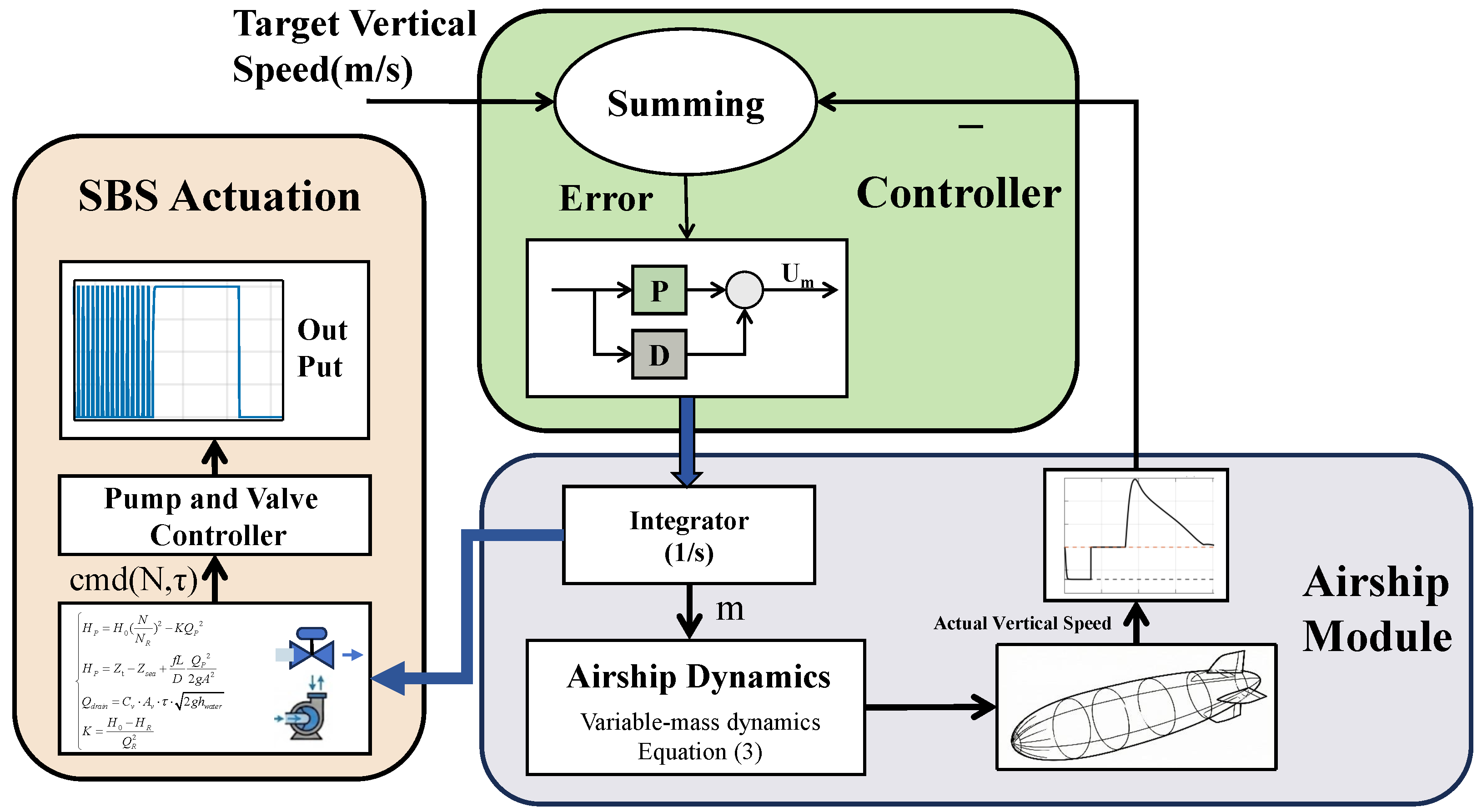
For the first-order local reduction described above, a PD controller C ( s ) = K p + K d s maps vertical-velocity error to the commanded mass-flow action U m ( s ) (Figure 3). The corresponding local closed-loop transfer function is
T ( s ) =   C ( s ) G ( s ) 1 + C ( s ) G ( s ) =   g ( K d s + K p ) / M ref s 2 + ( D + g K d ) s / M ref + g K p / M ref .

3.2. Preparation Phase for Flight Resumption: Cascade Control Based on Inverse Dynamics

After payload release and ballast rebalancing, the flight-resumption controller uses cascaded altitude and pitch loops. The simulation code labels this phase Go-Around (CLIMB). The altitude channel schedules total drain flow from the mass required for the bounded climb profile, while the pitch channel requests a pitch moment. These two targets are mapped to front and rear drain flows by a bounded active-set least-squares allocator. The allocator enforces nonnegative flow, valve-capacity, remaining-volume, and command-rate constraints and reports the achieved target vector and residual.

3.2.1. Cascaded Loop Architecture

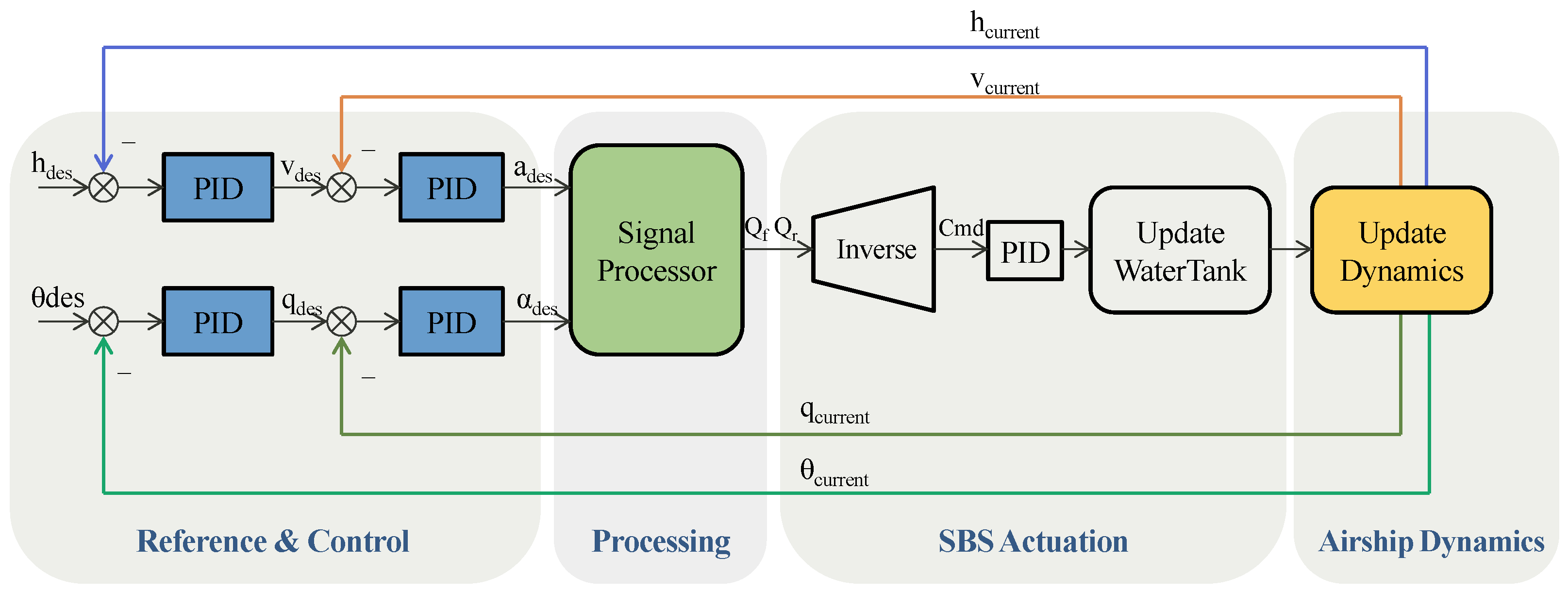
Figure 4 summarizes the cascaded control loops and the ballast-actuation path for flight resumption.
The Outer Loop (Trajectory/Attitude) is responsible for the management of slow dynamics. The function of the altitude controller is to output the desired vertical velocity ( V des ), while the pitch controller’s role is to output the desired pitch angular velocity ( q des ). The Inner Loop (Rate/Acceleration) is responsible for the management of rapid dynamics. The vertical velocity controller is responsible for generating the desired vertical acceleration ( a des ), while the pitch angular velocity controller is responsible for generating the desired angular acceleration ( α des ).

3.2.2. Inverse Dynamics and Control Allocation

The desired accelerations a des and α des serve as virtual control inputs. The vertical inverse-dynamics force is retained as a diagnostic, but a drain-only ballast actuator cannot act as a reversible vertical-force source because drainage also removes mass permanently. The implemented altitude channel therefore schedules total drainage from the mass balance, while the pitch channel computes the required moment:
F z = m current a des M y = I y y , current α des
With a bounded reference acceleration a ref and drainage horizon T d , the implemented mass schedule is
m sched = m neutral + m current a ref g , Q Σ , req = clip m current m sched ρ w T d , 0 , Q max .
Let b = [ Q Σ , req , M y , drain ] T collect the requested total drain flow and pitch moment, and let A ( h ) denote the state-dependent effectiveness matrix. The drain-flow vector minimizes the weighted total-flow/pitch-moment allocation residual and command-rate penalty subject to the declared physical bounds.
1 1 C front L C rear L Q front Q rear = Q Σ , r e q M y , d r a i n .
Here C front and C rear are the level-dependent drain-jet reaction coefficients; C i = ρ w 2 g h i at the current tank head h i , so that C i Q i is the jet reaction force of drain flow Q i , and C i L Q i is the corresponding pitch moment about the symmetric tank lever arm L; this state dependence is the A ( h ) introduced above.
Because only two drain actuators are used, all nine lower/free/upper active sets are enumerated. This prevents negative drainage commands and permits explicit reporting of saturation and allocation error.
Laguerre-parameterized predictive allocation [26] was considered, but it is not used or evaluated in the reported flight results. For the present instantaneous two-actuator problem, enumeration of the nine active sets gives the constrained optimum directly; the Laguerre basis primarily benefits long-horizon predictive formulations with many decision variables.

3.2.3. Actuator Dynamics

The lower-level flow loops use the SBS hydrodynamic model, including the pump curves, valve-flow characteristics, and pipe resistance, to calculate the pump speed and valve openings required for Q front and Q rear .
Independent PID loops track the commanded pump speed and valve openings using the corresponding actuator feedback signals.

3.3. Performance Analysis

The controller parameters used in every reported rerun are listed in Table 2 and match the archived run configuration.

Scope of the Control Analysis

The implemented closed loop is nonlinear, time-varying, hybrid across mission phases, and subject to tank, valve, pump, acceleration, and allocation limits. Consequently, a frozen transfer function and Routh table alone cannot establish global asymptotic stability. For the descent-speed loop, freezing the parameters and neglecting saturation gives the diagnostic pole s = K p V / ( 1 + K d V ) = 0.4 s−1 for K p V = 0.8 and K d V = 1.0 ; this is a local scalar result rather than a certificate for the complete hybrid system. The numerical evidence defines an explicit tested envelope: the nominal case passes, all ten controller/inertia-sweep runs pass, and all 21 actuator-time-constant cases from 1.0 to 3.0 times nominal pass. The separate N = 20 , ± 5 % parameter-dispersion ensemble provides a local sensitivity record. All 20 plotted trajectories remain within the declared state bounds, but their altitude spread does not support uniform tracking. These results are not a formal global Lyapunov or ISS proof. Different airship configurations still require configuration-appropriate controller selection; no global transferability claim is made.

4. Simulation and Results

4.1. Simulation Setup

This section specifies the simulation architecture, airship properties, hydraulic and aerodynamic coefficients, actuator parameters, mission profile, and controller parameters. The listed values come from the source code and configuration scripts used for the reported simulations.
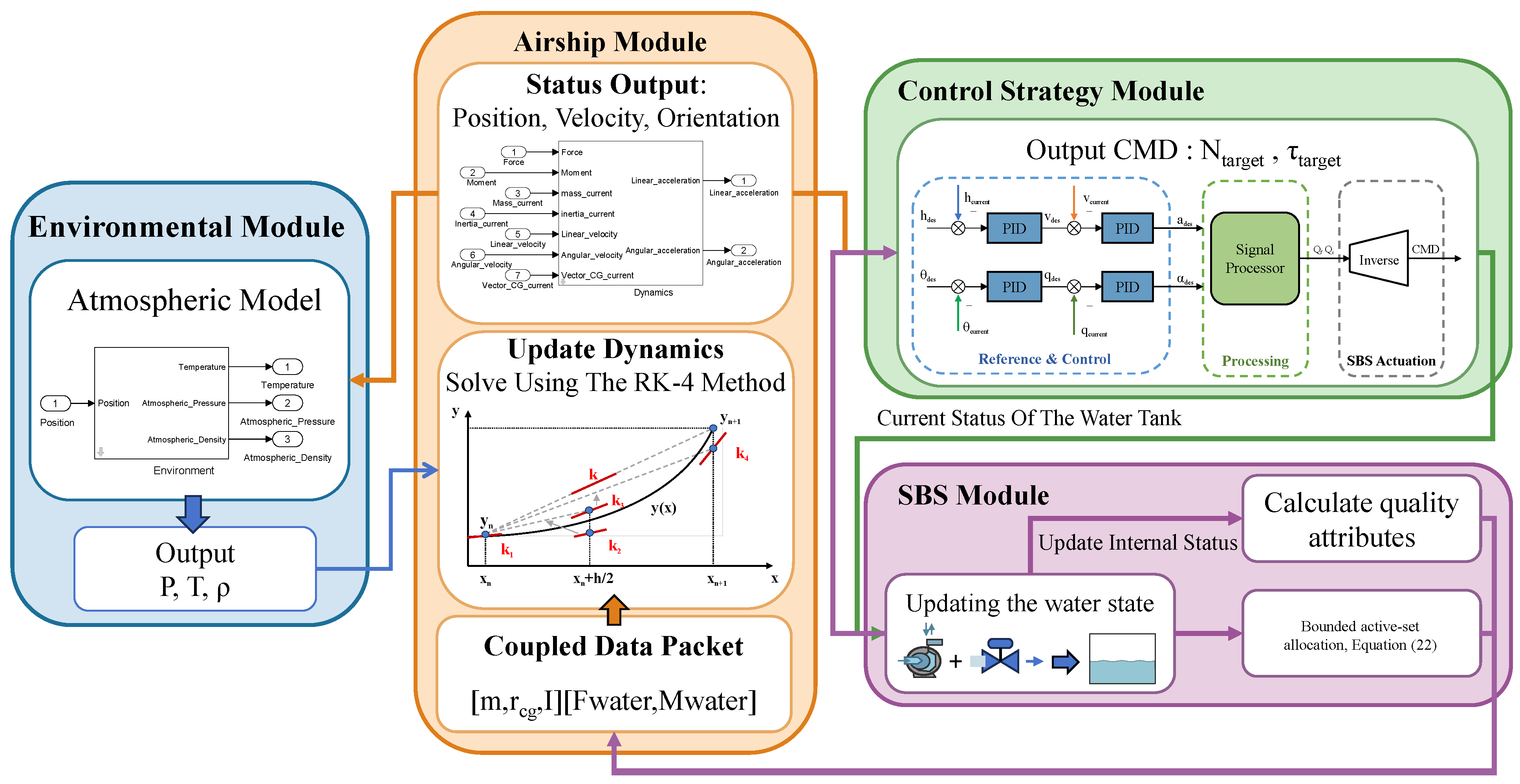
The numerical simulation uses MATLAB-compatible modular object-oriented code (Figure 5) that separates the airship, SBS, controller, and prescribed disturbance inputs. The reported cases were executed in GNU Octave 11.3. A five-second cross-platform regression against the archived MATLAB-compatible baseline was also retained. This organization supports repeatable numerical tests but does not by itself constitute experimental validation.
The airship parameters used in the simulation are listed in Table 3. The simplified pressure subsystem maintains a nominal envelope overpressure of 200 Pa and updates the modeled ballonet-air mass with altitude.
The fixed structure has a diagonal inertia tensor because the model assumes mass symmetry about its principal geometric axes. At each time step, the model updates the total inertia from the fixed structure, cargo, and three ballast masses. Their body-frame locations are r G o = [ 0 , 0 , 0.2 ] T m, r G c = [ 0 , 0 , 1.0 ] T m, r G 1 = [ 10 , 0 , 0.2 ] T m, r G 2 = [ 0 , 0 , 0.4 ] T m, and r G 3 = [ 10 , 0 , 0.2 ] T m.
The added-mass and added-inertia matrices are block-diagonal, as shown in Equations (23) and (24). To state the archived parameterization dimensionally, let ρ A , ref = 0.089 kg/m3, k 1 = 0.10 , k 2 = 0.87 , and 3 2 = 0.61 m2. All inertia quantities are referenced to the fixed body origin unless stated otherwise.
M add = ρ A , ref V diag ( k 1 , k 2 , k 2 ) .
I add = ρ A , ref V diag ( 0 , 3 2 , 3 2 ) .
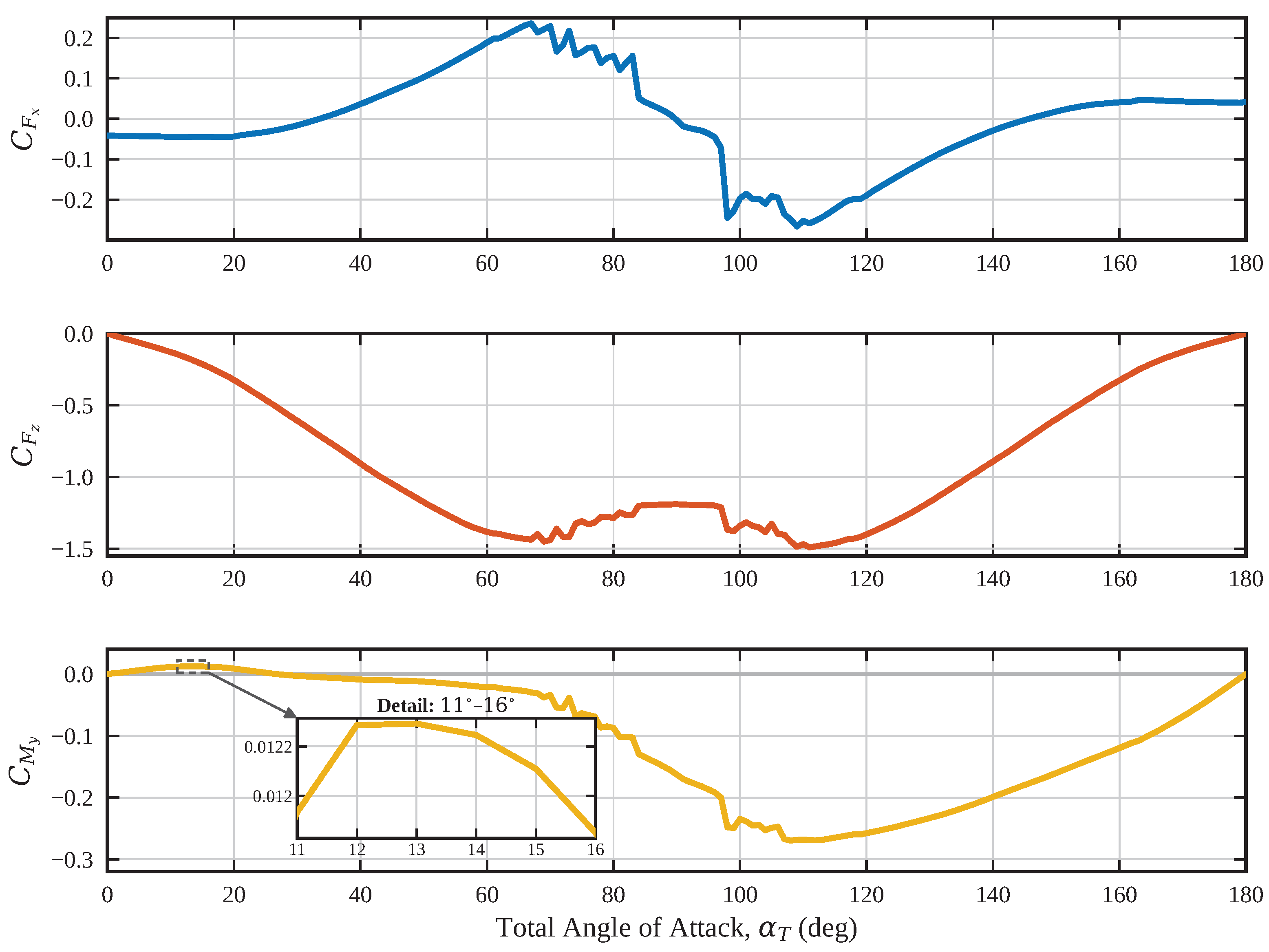
The lookup tables span a total-angle-of-attack range of 0– 180 . Figure 6 shows the longitudinal force and pitch-moment coefficients used by the model; the inset resolves the local variation near 12– 13 .
The SBS parameters are listed in Table 4.
Table 5 presents the task objectives and acceptance criteria established for this study.

4.2. Simulation Result Analysis

4.2.1. Nominal Coupled Mission and Property Evolution

Figure 7, Figure 8, Figure 9 and Figure 10 organize the mission evidence into ballast actuation, center-of-gravity migration, inertia evolution, and closed-loop flight response. Figure 7, Figure 8 and Figure 9 read the corrected 1201 s nominal-run log directly. Figure 10 retains the submitted proposed-controller mission history, which follows the original 1000 s profile, and reproduces it as vector artwork.
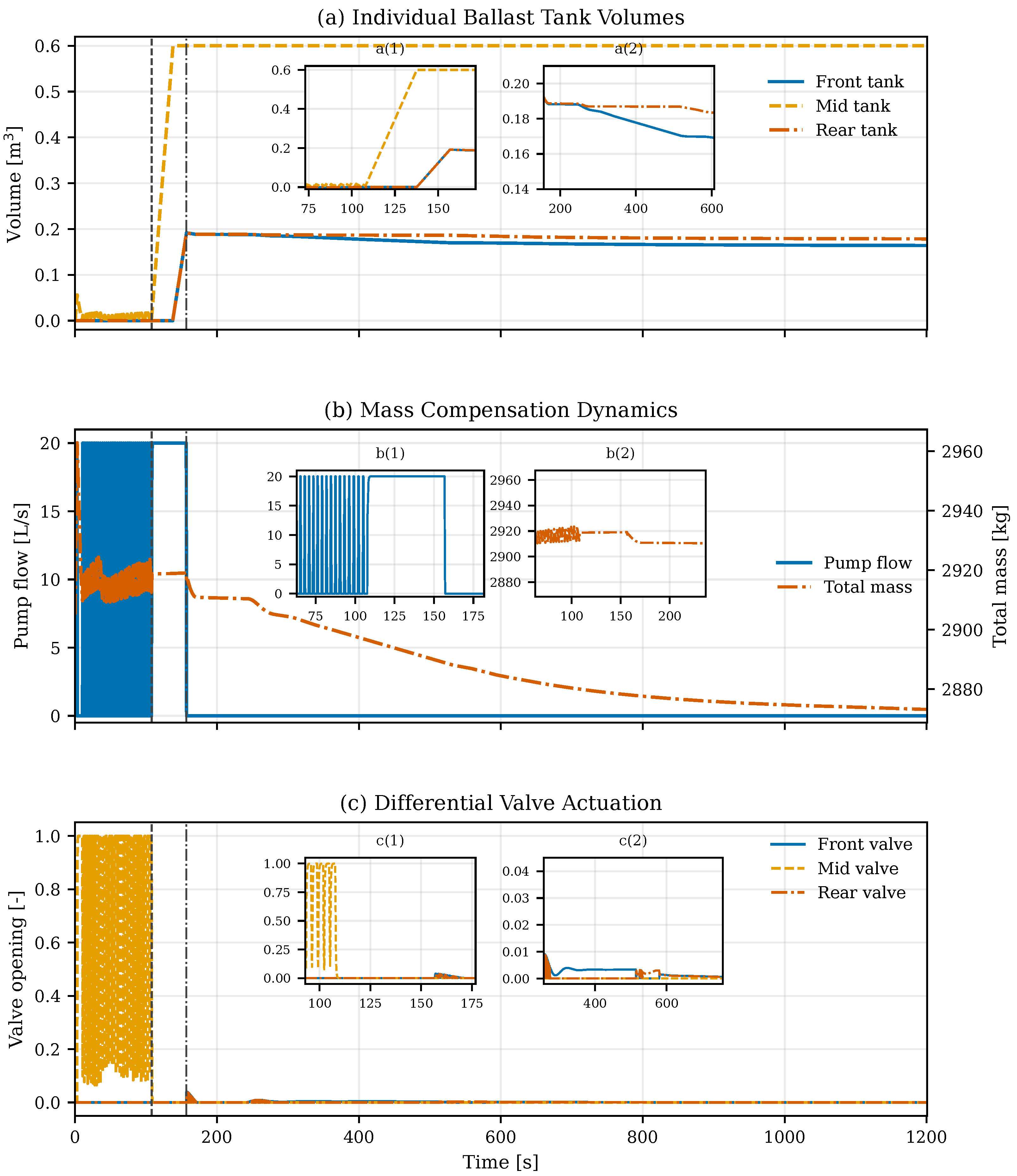
Figure 7 shows the ballast and mass-exchange histories in a three-panel layout. The middle tank reaches its 0.6 m3 capacity first. The front and rear tanks then provide the remaining longitudinal compensation.
During the cargo-transfer interval, bounded by the two event lines, the mission removes 996.58 kg of cargo while the logged seawater inventory rises to a comparable magnitude. The final ballast-water mass is 965.97 kg. Its subsequent gradual decrease reflects the controller’s trim correction. The transfer interval represents a modeled mission phase and does not imply instantaneous hydraulic compensation of an impulsive mass change.
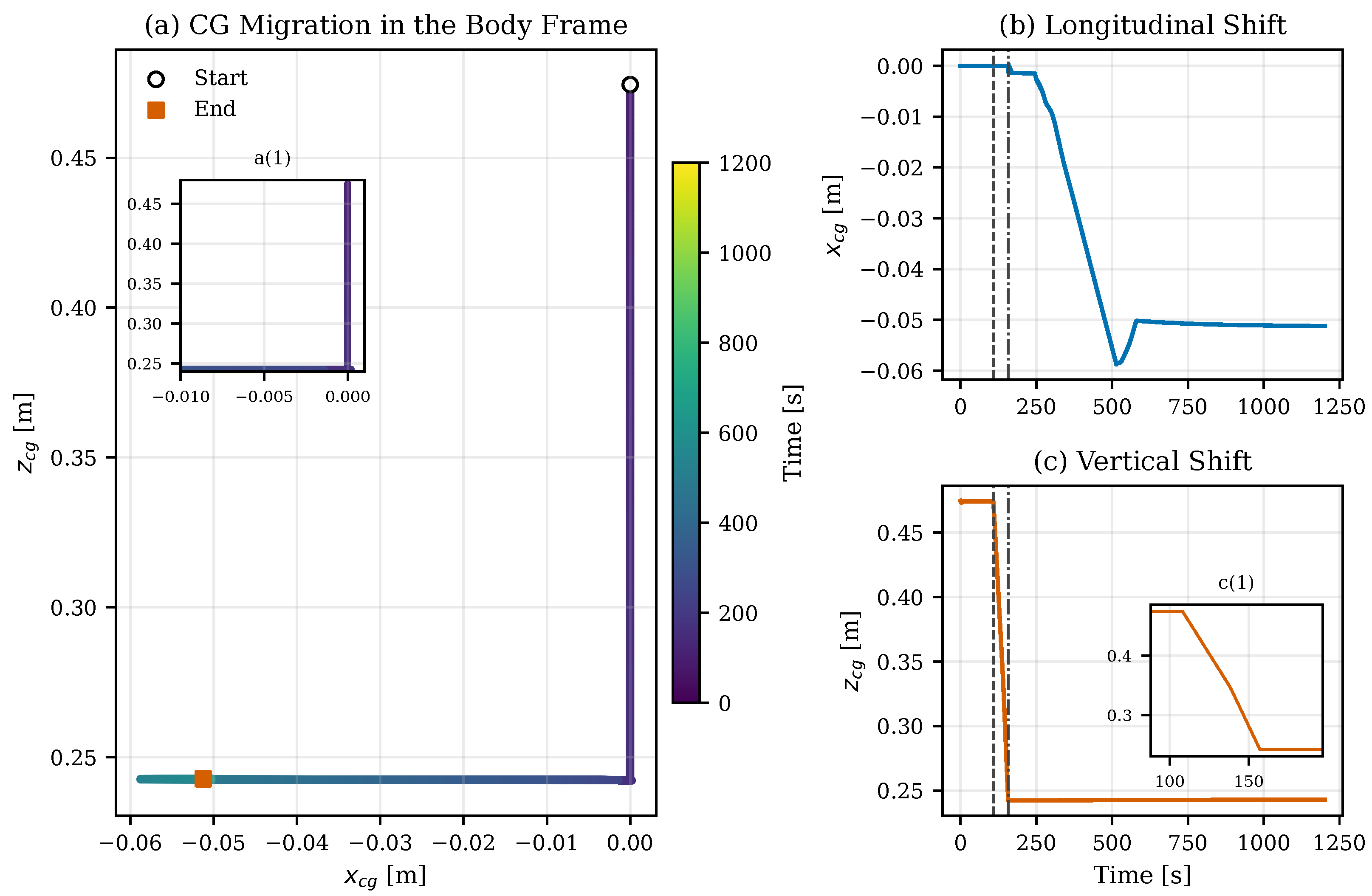
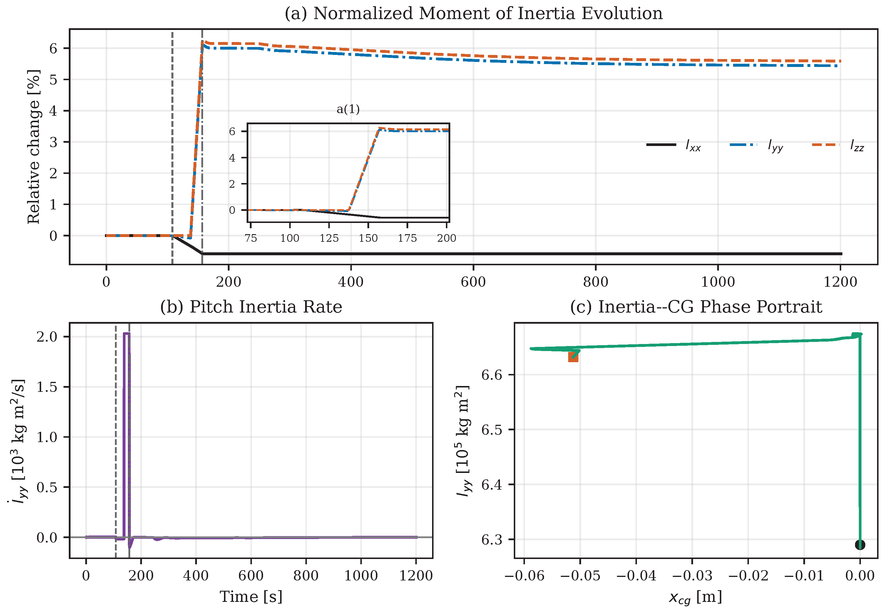
The same exchange moves the body-frame center of gravity and changes the rotational inertia. Figure 8 gives the complete logged CG path: x cg changes by 51.23 mm, z cg by 231.60 mm, and y cg remains zero because the present longitudinal model and tank layout are laterally symmetric. Figure 9 then shows that I y y and I z z increase by 5.44% and 5.59%, respectively, whereas I x x decreases by 0.59%. The maximum resolved magnitude of I ˙ y y is 2030.33 kg m2/s. These histories provide the direct numerical link between ballast redistribution and the variable-property terms retained in the dynamics; they are not interpreted as structural-response measurements.
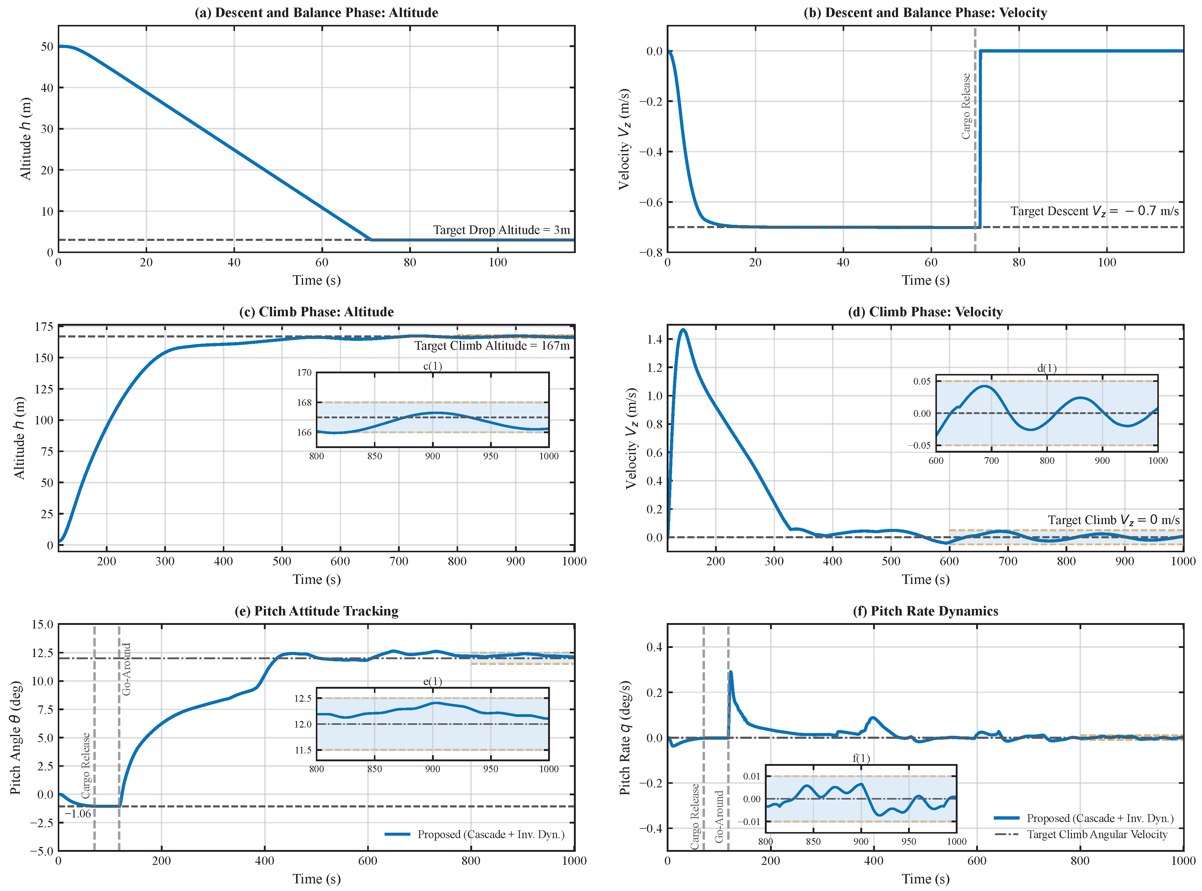
Figure 10 retains the proposed controller’s submitted mission history in the original six-panel layout. It provides a qualitative view of descent, balance, and flight resumption, while four insets resolve the terminal altitude, vertical-velocity, pitch-angle, and pitch-rate histories. This figure is used only to document the proposed controller. Table 6 and the inertia sweep in Section 4.2.3 provide the corrected 1201 s common-protocol comparison and quantitative controller ranking.
The rigid-body/hydraulic model contains no structural dynamics, and its 10 Hz flight-level log cannot resolve a 7 Hz structural response. The evidence therefore covers hydraulic pressure and force excitation together with rigid-body motion, but it does not identify a structural resonance or fatigue margin. Each regenerated curve is traceable to its archived simulation log and plotting script.

4.2.2. MOC Reference and Reduced-Model Verification

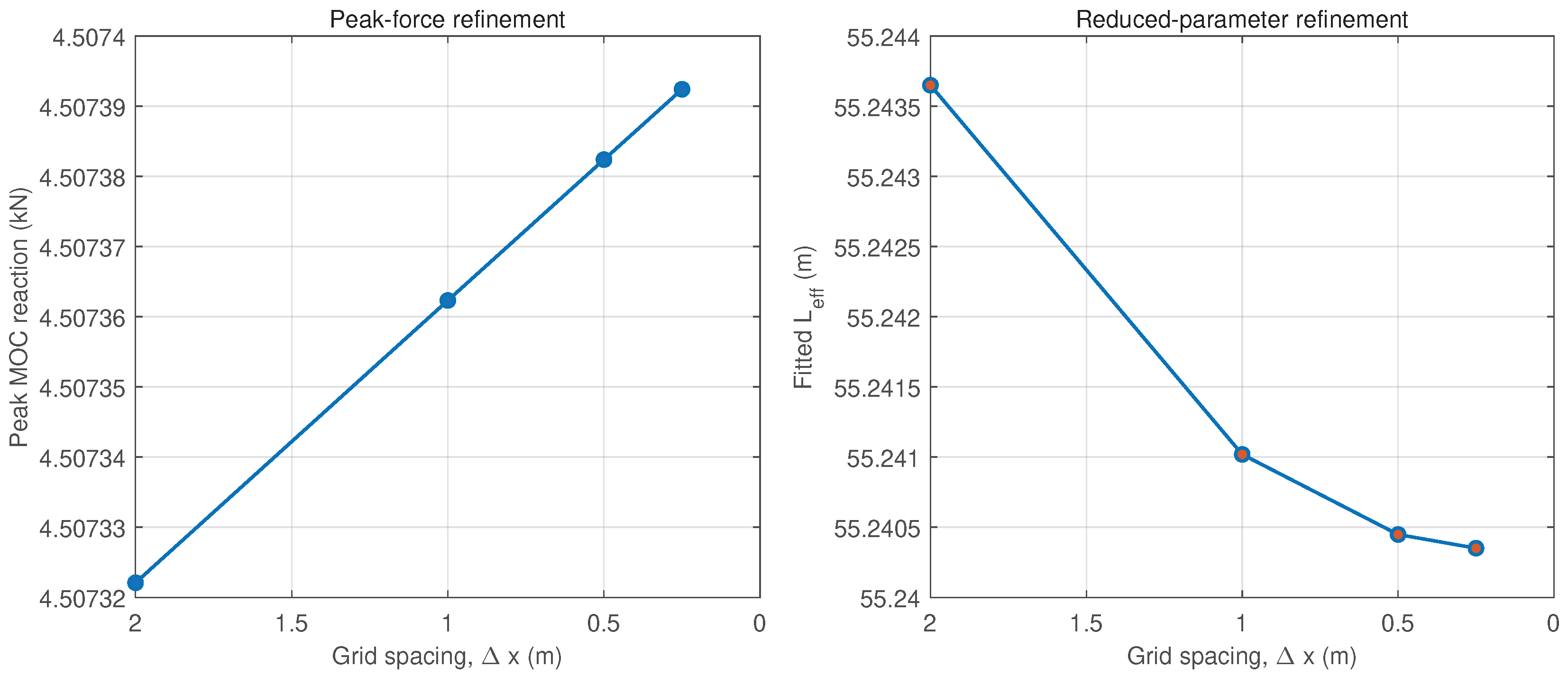
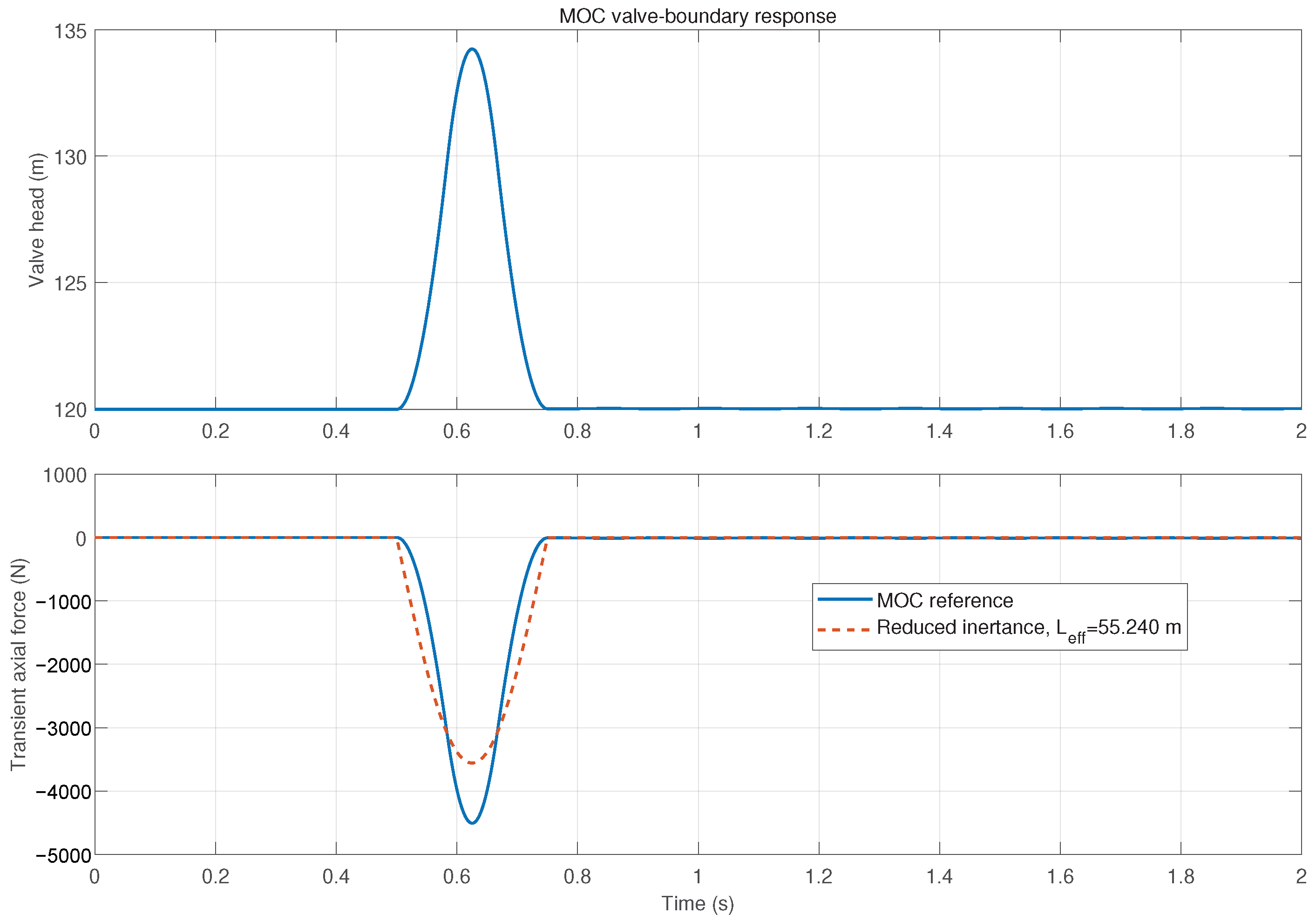
The CFL-one refinement uses 25, 50, 100, and 200 cells. Relative to the 200-cell calculation, the 100-cell peak reaction differs by 2.22 × 10 4 % and the fitted L eff by 1.77 × 10 4 % (Figure 11). For the declared 0.25 s valve transition, the 100-cell MOC reference gives a peak axial reaction of 4.507 kN. The fitted reduced model gives 3.558 kN, underpredicting the peak by 21.1%. Its full-record root-mean-square error (RMSE) is 244.4 N, and its closure-interval normalized RMSE (NRMSE) is 15.3%. Figure 12 shows that the reduced relation captures the integrated flight-level load trend but does not reproduce the complete pressure-wave waveform. It is therefore retained as a reduced runtime approximation, not presented as a validated replacement for distributed hydraulics.

4.2.3. Fair Controller Ablation and Allocation Feasibility

The fair comparison changes only the variable-property compensation: the ablation freezes the nominal pitch inertia and omits the associated correction, while retaining the same nonlinear plant, hydraulic model, actuator dynamics, constrained allocator, limits, commands, and logging. Table 6 shows that both cases satisfy the nominal predeclared criteria. The variable-property-aware case has a 2.985 m final-altitude error and a 0.165 steady-climb pitch RMS error; the frozen-inertia case gives 2.806 m and 0.157 , respectively. Thus the frozen-inertia case is slightly better in both nominal terminal metrics; the variable-property-aware pitch RMS is 5.1% higher. The nominal comparison alone does not support a controller-superiority claim.
The controller ranking uses only the common-protocol nominal comparison and the declared inertia sweep. Deliberately severe fixed-model mismatch cases are excluded from the main evidential chain because they do not provide a fair generic PID benchmark.
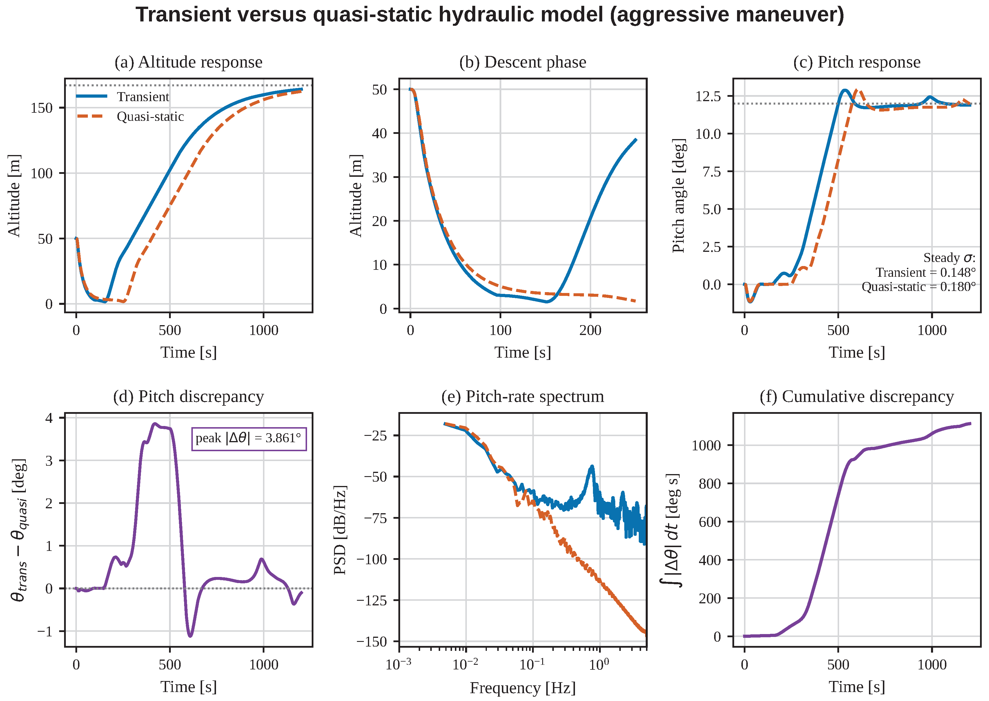
Figure 13 compares the independently logged transient-hydraulic and quasi-static responses under the same aggressive maneuver.
The aggressive transient-hydraulic case also passes, with 2.954 m altitude error, 0.149 pitch RMS, zero capacity-saturation fraction, a 0.00715 95th-percentile weighted allocation residual, and a brief maximum residual of 1.124 at t = 150.2 s. The corresponding aggressive quasi-static case gives 4.576 m, 0.204 , zero saturation, a 0.00736 residual 95th percentile, and a 0.00991 maximum. The reported residual is the allocator’s dimensionless weighted total-flow/pitch-moment norm. A separate rate-limit fraction was not retained in the batch log and is therefore not claimed.
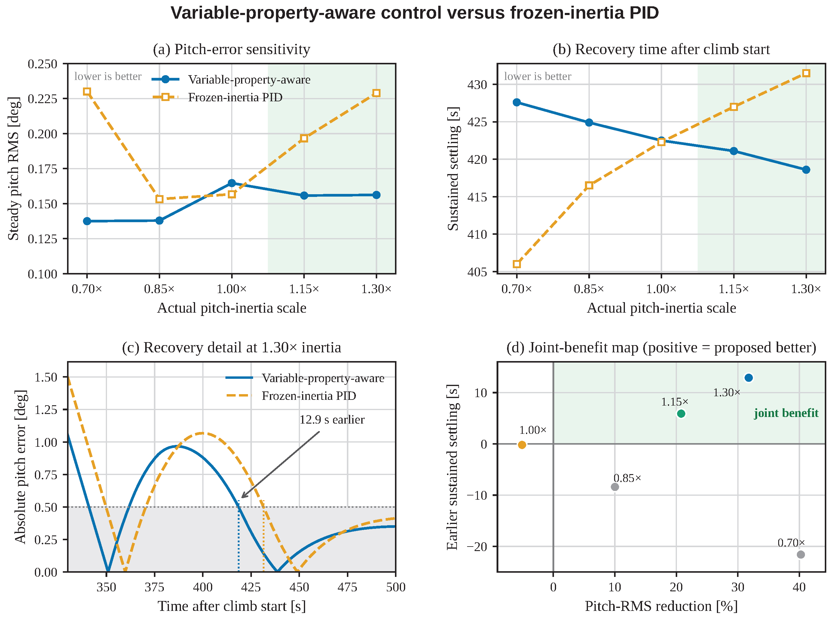
To test the specific benefit of updating the mass properties rather than selecting a favorable nominal point, we additionally prescribed a five-point structural pitch-inertia sweep at 0.70, 0.85, 1.00, 1.15, and 1.30 times the nominal value. The five multipliers form a symmetric numerical sensitivity grid, with ± 15 % interior points and ± 30 % endpoints; they are not measured configuration tolerances. The nonlinear plant, mission, hydraulic model, gains, actuator dynamics, allocator, constraints, and calm environment are identical in all ten runs. The variable-property-aware controller uses the current simulated inertia and exchange-moment terms; the frozen-inertia PID uses a single nominal post-transfer inertia of 6.674 × 10 5 kg m2 in every run. All ten cases satisfy the predeclared nominal acceptance criteria. The variable-property-aware controller gives lower steady-climb pitch RMS at 0.70, 0.85, 1.15, and 1.30 times nominal inertia, whereas the frozen-inertia PID is slightly better at 1.00 times nominal. This RMS comparison is not uniformly accompanied by faster recovery: at 0.70 and 0.85 times nominal, the variable-property-aware case reaches the sustained ± 0.5 band 21.6 and 8.4 s later, respectively. The high-inertia results are aligned across the recovery metrics. At 1.15 times nominal, the variable-property-aware controller reduces pitch RMS from 0.197 to 0.156 and settles 5.9 s earlier. At 1.30 times nominal, it reduces pitch RMS from 0.229 to 0.156 (31.8%) and settles 12.9 s earlier (418.6 versus 431.5 s after climb initiation); the terminal altitude errors are 2.741 and 2.899 m, respectively. Figure 14 displays every tested point and the upper-end trajectory. Across the tested grid, the variable-property-aware controller is also markedly less sensitive to the inertia level: its steady-climb pitch RMS error stays within 0.137 0.165 while the frozen-inertia PID spans 0.153 0.230 , its worst tested-point RMS error is 28.4% lower, and its settling-time spread across the sweep is 9.0 s versus 25.5 s. The result supports a bounded high-inertia compensation advantage together with this reduced sensitivity over the tested range, not uniform per-point superiority over the frozen-inertia PID.

4.2.4. Actuator-Time-Constant Sweep

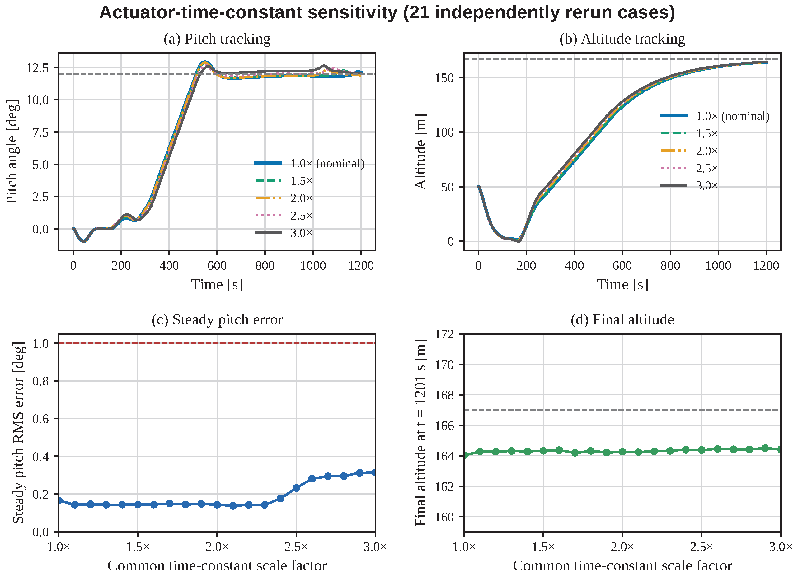
Figure 15 summarizes the actuator-time-constant sweep. The pump and valve first-order time constants are scaled jointly by a common factor γ { 1.0 , 1.1 , , 3.0 } from their nominal values T c , p = 0.10 s and T c , v = 0.15 s. Each value of γ is an independent rerun; the two time constants are not varied independently of one another. A case passes only if it reaches the flight-resumption phase (Phase 4), final altitude error is at most 5 m, steady-climb pitch RMS error is at most 1 , valve-capacity saturation occurs in at most 10% of valid samples, all states remain finite, maximum absolute pitch is at most 45 , and maximum absolute altitude is at most 1000 m. All 21 cases pass. Across the sweep, the worst pitch RMS error is 0.315 , the worst altitude error is 2.985 m, and no capacity-saturation sample is logged. The largest tested passing factor is therefore 3.0; no claim is made beyond the tested interval. The nonmonotonic RMS variation also cautions against interpreting actuator lag as the only source of closed-loop error.

4.2.5. Local Parameter-Dispersion Study

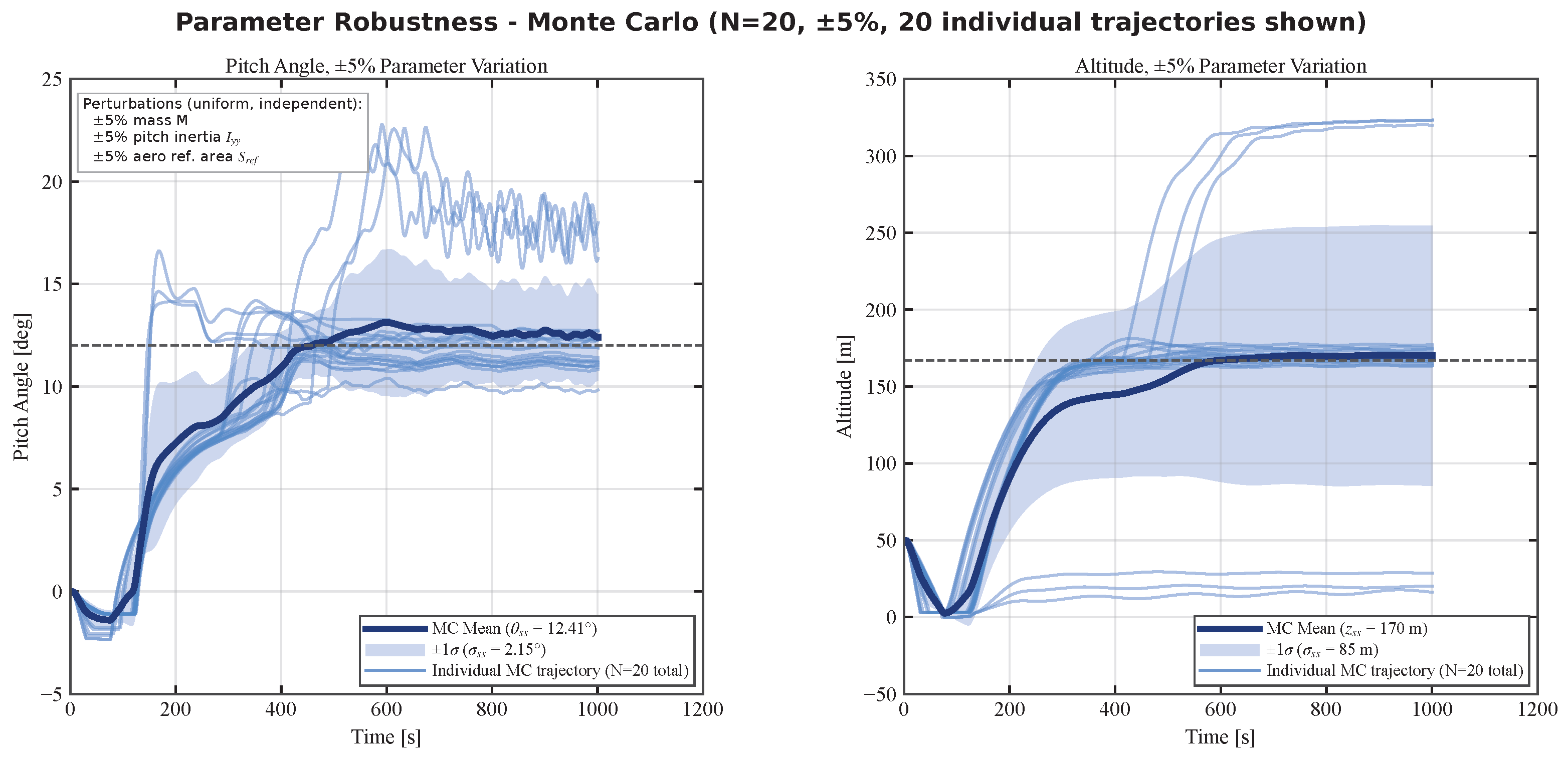
Figure 16 shows the local parameter-dispersion ensemble. The local parameter-dispersion study uses N = 20 realizations with independent uniform ± 5 % changes in structural mass, pitch inertia, and aerodynamic reference area while preserving the matched controller, actuator model, mission, and calm environment. All 20 plotted trajectories remain finite and within the declared state-boundedness limits. The ensemble has a terminal pitch mean of 12.41 with a 2.15 standard-deviation band and an altitude mean of 170 m with an 85 m standard-deviation band. The altitude spread shows that boundedness is not equivalent to uniform tracking performance.
The N = 20 ensemble is therefore described as a local sensitivity illustration rather than a statistically converged reliability estimate. The ± 5 % interval is a declared neighborhood of the matched airship configuration, not a universal manufacturing or environmental distribution. Actuator uncertainty is assessed separately by the 21 independently rerun common time-constant scale factors in Figure 15. This separation avoids conflating plant dispersion, actuator lag, and an unvalidated maritime disturbance model in a single pass/fail statistic.

4.2.6. Dimensionless Design Screening

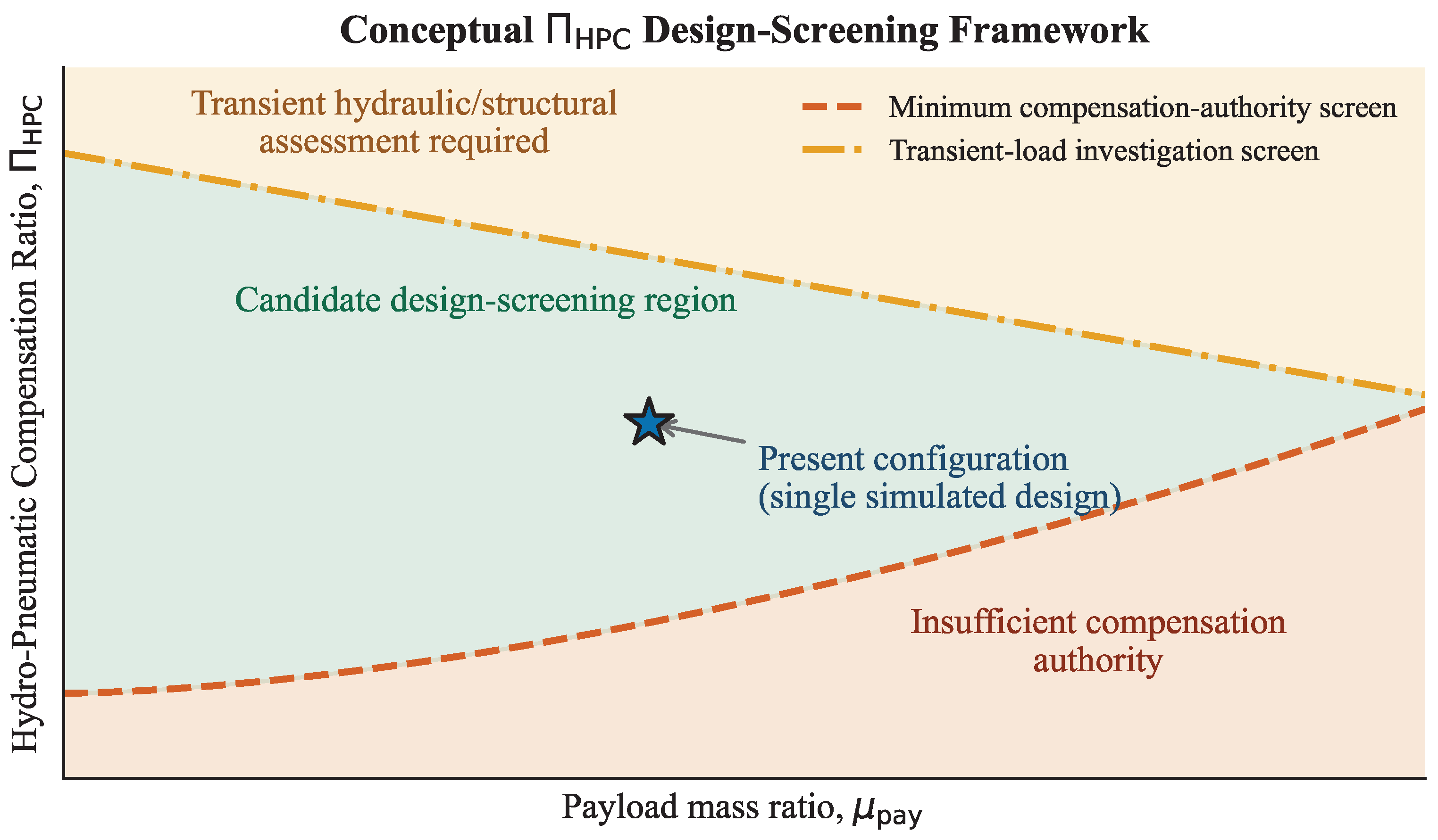
To retain the useful sizing interpretation, we define the hydro-pneumatic compensation ratio as
Π HPC = ρ w Q max τ resp M cargo .
The ratio measures the ballast mass transferable over a characteristic response time relative to the released payload mass. A small value indicates insufficient compensation authority. Increasing Q max also increases the transient hydraulic load that the pressure model must assess. Figure 17 presents this trade-off as a conceptual screening framework. Its two curves are qualitative hypotheses, and the single simulated design point does not establish fitted stability or FSI-safety boundaries for other airship/controller pairs.

4.3. Limitations

This study is simulation-only. It does not include experimental hydraulic validation, tank sloshing, a resolved pump-inlet turning geometry, validated wave/suction interaction, structural or fluid–structure response, stress/fatigue analysis, sensor and estimator dynamics, hardware-in-the-loop testing, or flight testing. Robust adaptive disturbance estimation and saturation-aware path-following methods [27,28], together with passivity-based formulations for strongly coupled unmanned aerial platforms [29], are relevant alternatives, but they are not implemented or evaluated here. The Π HPC ratio and Figure 17 are therefore a conceptual sizing framework, not validated stability or structural-safety boundaries. The local pole check, nominal run, ten inertia-sweep runs, and 21 actuator-time-constant cases establish a tested numerical envelope rather than global asymptotic stability. The local-dispersion ensemble supports only a matched-configuration boundedness statement. Configuration-specific buoyancy/trim and controller rematching, lateral–directional disturbance rejection, and a validated wind/wave interface model remain necessary before extrapolating beyond that envelope.

5. Conclusions

This study presents a variable-property flight-dynamics formulation and constrained ballast-flow allocation framework for a simulated unmanned cargo airship. Under the nominal 1201 s mission, the variable-property-aware case meets the altitude, pitch, saturation, and boundedness criteria, with 2.985 m final-altitude error and 0.165 pitch RMS error. The fair frozen-inertia ablation also passes and produces slightly lower nominal errors (2.806 m and 0.157 ), so nominal superiority is not claimed. The controlled inertia sweep nevertheless identifies an aligned high-inertia benefit: at 1.30 times nominal inertia, the variable-property-aware controller reduces pitch RMS from 0.229 to 0.156 (31.8%) and settles 12.9 s earlier. Across the full 0.70–1.30 sweep, variable-property compensation also keeps the pitch RMS error within 0.137 0.165 , whereas the frozen-inertia PID varies between 0.153 and 0.230 ; because cargo and ballast loading differ between missions, this low sensitivity to the inertia level, rather than performance at a single matched nominal point, is the practically relevant benefit of variable-property compensation. All 21 tested actuator-time-constant factors up to 3.0 times nominal pass. The N = 20 , ± 5 % local parameter-dispersion ensemble remains state-bounded, while its wide altitude spread precludes a uniform tracking or reliability claim. The reduced hydraulic model gives a 15.3% closure-interval NRMSE against the independent MOC reference and is treated as a flight-level approximation rather than experimental validation.
The supported conclusion is therefore deliberately conditional. Synchronized ballast transfer and constrained allocation are numerically feasible for the declared nominal, inertia-variation, and actuator-time-constant cases. The local dispersion ensemble provides a matched-configuration sensitivity record and does not establish uniform tracking. Hydraulic experiments, configuration-specific buoyancy/trim and controller rematching, a structural/FSI model with adequate sampling, hardware-in-the-loop tests, and flight validation remain necessary before extending the present simulation evidence to structural safety, global stability, or operational readiness.

Author Contributions

Conceptualization, D.G. and D.Z.; methodology, H.C., H.H., D.G. and D.Z.; software, H.C. and H.H.; validation, H.C., H.H. and C.F.; formal analysis, H.C. and H.H.; investigation, H.C. and H.H.; resources, C.F., D.G., D.Z., H.W. and Y.W.; data curation, H.C. and H.H.; writing—original draft preparation, H.C.; writing—review and editing, H.C., C.F., H.H., D.G., D.Z., H.W. and Y.W.; visualization, H.C. and H.H.; supervision, C.F., D.G., D.Z., H.W. and Y.W.; project administration, D.G. and D.Z.; funding acquisition, D.G. and D.Z. All authors have read and agreed to the published version of the manuscript.

Funding

This work was supported by the Fundamental Research Funds for the Central Universities (502GWXM2026129001) and the Fundamental and Interdisciplinary Disciplines Breakthrough Plan of the Ministry of Education of China (JYB2025XDXM115).

Data Availability Statement

The original contributions presented in this study are included in the article. Further inquiries can be directed to the corresponding author.

Conflicts of Interest

Author Daliang Gao was employed by Linzhou (Ningbo) Technology Co., Ltd. The remaining authors declare that the research was conducted in the absence of any commercial or financial relationships that could be construed as a potential conflict of interest.

References

  1. Prentice, B.E.; Lau, Y.-Y.; Ng, A.K.Y. Transport Airships for Scheduled Supply and Emergency Response in the Arctic. Sustainability 2021, 13, 5301. [Google Scholar] [CrossRef] [Scilit]
  2. Guy, D. The Logistics of International Emergency Relief: Are Airships the Solution? Humanitarian Practice Network. 17 March 2014. Available online: https://odihpn.org/en/publication/the-logistics-of-international-emergency-relief-are-airships-the-solution/ (accessed on 12 September 2026).
  3. Prentice, B.E.; Knotts, R. Cargo Airships: International Competition. J. Transp. Technol. 2014, 4, 187–195. [Google Scholar]
  4. Carichner, G.E.; Nicolai, L.M. Fundamentals of Aircraft and Airship Design: Volume 2—Airship Design and Case Studies; AIAA: Reston, VA, USA, 2013. [Google Scholar]
  5. Yan, F.; Huang, W.N.; Yang, Y.C.; Zhu, R.C. Overview of Developing Status Quo and Trend of Modern Heavy Lift Airships. Sci. Technol. Rev. 2017, 35, 68–80. [Google Scholar]
  6. Pasternak, I. Flight System for a Constant Volume, Variable Buoyancy Air Vehicle. U.S. Patent 9,016,622 B1, 28 April 2015. Available online: https://patents.google.com/patent/US9016622B1/en (accessed on 29 August 2026).
  7. Norris, G. Lockheed Martin Readies LMH-1 Hybrid Airship Assembly. Aviation Week & Space Technology. 16 March 2016. Available online: https://aviationweek.com/air-transport/lockheed-martin-readies-lmh-1-hybrid-airship-assembly (accessed on 29 August 2026).
  8. Andan, A.D.; Asrar, W.; Omar, A.A. Investigation of Aerodynamic Parameters of a Hybrid Airship. J. Aircr. 2012, 49, 658–662. [Google Scholar] [CrossRef] [Scilit]
  9. Gao, W.; Bi, Y.; Li, X.; Dong, A.; Wang, J.; Yang, X. Variational Method-Based Trajectory Optimization for Hybrid Airships. Aerospace 2024, 11, 250. [Google Scholar] [CrossRef] [Scilit]
  10. Murugaiah, M.; Pant, R.S. Surrogate Based Aerodynamic Shape Optimization of Tri-Lobed Hybrid Airship Envelope. In Proceedings of the AIAA Aviation Forum, Virtual, 2–6 August 2021. [Google Scholar] [CrossRef] [Scilit]
  11. Hexcel Corporation. Flying Whales Selects Hexcel for the Supply of Composites Materials for Its LCA60T Airship. Press Release. 20 June 2025. Available online: https://www.hexcel.com/News/News-Releases/5753/flying-whales-selects-hexcel-for-the-supply-of-composites-materials-for-its-lca60 (accessed on 1 September 2026).
  12. Guo, Q.; Zhou, J.; Li, Y.; Guan, X.; Liu, D.; Zhang, J. Fluid-Structure Interaction Response of a Water Conveyance System with a Surge Chamber during Water Hammer. Water 2020, 12, 1025. [Google Scholar] [CrossRef] [Scilit]
  13. Tijsseling, A.S. Fluid-Structure Interaction in Liquid-Filled Pipe Systems: A Review. J. Fluids Struct. 1996, 10, 109–146. [Google Scholar] [CrossRef] [Scilit]
  14. Wiggert, D.C.; Tijsseling, A.S. Fluid Transients and Fluid-Structure Interaction in Flexible Liquid-Filled Piping. Appl. Mech. Rev. 2001, 54, 455–481. [Google Scholar] [CrossRef] [Scilit]
  15. Harada, K.; Eguchi, K.; Sano, M.; Sasa, S. Experimental Study of Thermal Modeling for Stratospheric Platform Airship. In Proceedings of the AIAA’s 3rd Annual Aviation Technology, Integration, and Operations (ATIO) Tech. Forum, Denver, CO, USA, 17–19 November 2003. [Google Scholar]
  16. Liu, Q.; Yang, Y.; Cai, J.; Zhu, R.; Cui, Y. An experimental investigation into the thermal performance of sphere balloon. In Proceedings of the 37th Chinese Control Conference (CCC), Wuhan, China, 25–27 July 2018; pp. 9918–9921. [Google Scholar]
  17. Cai, Z.; Qu, W.; Xi, Y. Dynamic modeling for airship equipped with ballonets and ballast. Appl. Math. Mech. 2005, 26, 1072–1082. [Google Scholar] [CrossRef] [Scilit]
  18. Hansen, E.L.M.B.; Silva, F.M.A. Nonlinear Vibration Analysis of a Partially Filled Multi-Layer Cylindrical Tank: Consideration of the Sloshing Effects in the Fluid–Structure Interaction. J. Braz. Soc. Mech. Sci. Eng. 2022, 44, 484. [Google Scholar] [CrossRef] [Scilit]
  19. Li, Y.; Nahon, M.; Sharf, I. Airship Dynamics Modeling: A Literature Review. Prog. Aerosp. Sci. 2011, 47, 217–239. [Google Scholar] [CrossRef] [Scilit]
  20. López, D.; Domínguez, D.; Delgado, A.; García-Gutiérrez, A.; Gonzalo, J. Experimental Calculation of Added Masses for the Accurate Construction of Airship Flight Models. Aerospace 2024, 11, 872. [Google Scholar] [CrossRef] [Scilit]
  21. Chaudhry, M.H. Applied Hydraulic Transients; Springer: New York, NY, USA, 2014. [Google Scholar]
  22. Wylie, E.B.; Streeter, V.L.; Suo, L. Fluid Transients in Systems; Prentice Hall: Englewood Cliffs, NJ, USA, 1993. [Google Scholar]
  23. Chen, L.; Zhou, G.; Yan, X.J.; Duan, D.P. Composite Control of Stratospheric Airships with Moving Masses. J. Aircr. 2012, 49, 794–801. [Google Scholar] [CrossRef] [Scilit]
  24. Salui, S.; Ghosh, A. Design and Real-Time Implementation of a 2-Rate Control in CPS-Like Environment. IEEE Trans. Aerosp. Electron. Syst. 2025, 61, 14374–14383. [Google Scholar] [CrossRef] [Scilit]
  25. Liu, S.; Zhou, S.; Miao, J.; Shang, H.; Cui, Y.; Lu, Y. Autonomous Trajectory Planning Method for Stratospheric Airship Regional Station-Keeping Based on Deep Reinforcement Learning. Aerospace 2024, 11, 753. [Google Scholar] [CrossRef] [Scilit]
  26. Valencia-Palomo, G.; Rossiter, J.A. Using Laguerre Functions to Improve Efficiency of Multi-parametric Predictive Control. In Proceedings of the 2010 American Control Conference (ACC), Baltimore, MD, USA, 30 June–2 July 2010. [Google Scholar]
  27. Wasim, M.; Ali, A.; Saleem, F.; Shaikh, I.U.H.; Iqbal, J. Robust Adaptive Control with Lumped Model Uncertainty and Wind Disturbance Estimation for Airship Trajectory Tracking. PLoS ONE 2025, 20, e0335392. [Google Scholar] [CrossRef]
  28. Zheng, Z.; Sun, L. Error-Constrained Path-Following Control for a Stratospheric Airship with Actuator Saturation and Disturbances. Int. J. Syst. Sci. 2017, 48, 3504–3521. [Google Scholar] [CrossRef] [Scilit]
  29. García-Beltrán, C.D.; Miranda-Araujo, E.M.; Guerrero-Sanchez, M.E.; Valencia-Palomo, G.; Hernández-González, O.; Gómez-Peñate, S. Passivity-Based Control Laws for an Unmanned Powered Parachute Aircraft. Asian J. Control 2021, 23, 2087–2096. [Google Scholar] [CrossRef] [Scilit]
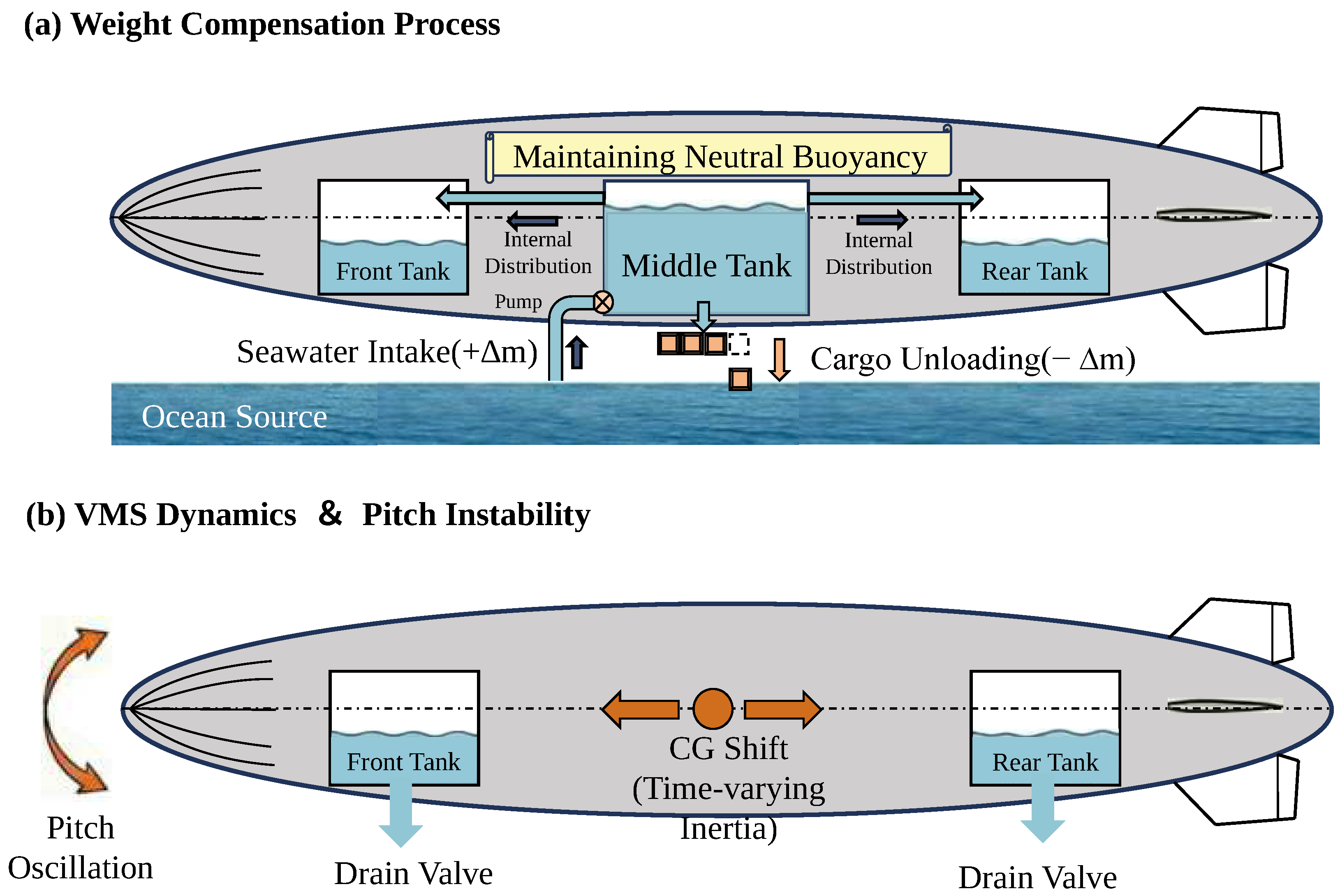
Figure 1. Operational concept of the active Seawater Ballast System (SBS). (a) Seawater intake compensates payload removal during low-speed cargo exchange. (b) During recovery, total drainage schedules mass removal, while differential front–rear drainage produces pitch moment and changes the mass, center-of-gravity location, and body-origin inertia. Blue denotes seawater and its transfer paths; orange identifies cargo removal and CG/pitch changes. Gray outlines depict the hull and tanks, and the longitudinal guide indicates their spatial arrangement. Arrows indicate the labeled flow or motion directions.
Drones 10 00704 g001
Figure 2. Coordinate system.
Drones 10 00704 g002
Figure 3. Control system design for the descent phase. The green region contains the vertical-velocity error calculation and PD controller; the peach region contains the pump/valve actuation path, and the lavender region contains the mass update and airship dynamics. Arrows show the command and feedback paths, and the negative feedback compares actual and target vertical speed. The embedded plots illustrate the signal locations; the quantitative mission histories are reported in the results section.
Drones 10 00704 g003
Figure 4. Cascaded altitude–pitch control and constrained ballast-flow allocation for the flight-resumption phase. Blue PID blocks form the altitude/vertical-velocity and pitch/pitch-rate cascades. The green signal processor produces the front/rear flow requests; the inverse-mapping, actuator PID, and water-tank blocks form the SBS actuation path. The yellow block updates airship dynamics. Circular junctions subtract the labeled feedback quantities; the colored return lines distinguish altitude, velocity, pitch-rate, and pitch feedback. Rounded background regions group the four labeled functional stages.
Drones 10 00704 g004
Figure 5. Modular simulation framework. The rigid-body and hydraulic runtime states are updated at 100 Hz, the controller at 50 Hz, and logs at 10 Hz. The runtime hydraulic term is a reduced line-inertance model; the independent MOC reference uses its own CFL-consistent grid and time step. Blue, orange, green, and purple regions identify the environmental, airship, control-strategy, and SBS modules, respectively. Arrows denote the labeled exchanges of atmospheric properties, vehicle state, actuator commands, tank state, mass properties, and water-induced forces/moments. Insets illustrate the corresponding module operations; the RK-4 inset denotes the time-integration stages.
Drones 10 00704 g005
Figure 6. Longitudinal aerodynamic coefficients vs. total angle of attack. The inset enlarges the explicitly marked 11 16 interval of C M y .
Drones 10 00704 g006
Figure 7. Nominal SBS actuation and mass exchange. (a) Individual tank volumes; (b) pump flow and total simulated mass; (c) differential valve openings. The dashed and dash-dotted vertical lines denote the start of cargo transfer and the flight-resumption phase, respectively; the insets show the corresponding local transients. In each panel, inset (1) enlarges the earlier filling or actuation interval, and inset (2) enlarges the later adjustment interval; the inset time axes specify the respective windows.
Drones 10 00704 g007
Figure 8. Center-of-gravity evolution in the nominal simulation. (a) Time-colored x cg z cg migration path; (b) longitudinal CG history; (c) vertical CG history. The lateral component remains zero under the symmetric longitudinal model.
Drones 10 00704 g008
Figure 9. Variable inertial properties in the nominal simulation. (a) Relative changes in the three principal inertias; (b) resolved pitch-inertia rate; (c) coupled I y y x cg phase portrait. The plotted rate is obtained by differentiating the logged inertia history at the 10 Hz output rate.
Drones 10 00704 g009
Figure 10. Submitted mission history of the variable-property-aware controller, reproduced as vector artwork. (a,b) Descent/balance altitude and vertical velocity; (c,d) flight-resumption altitude and vertical velocity; (e,f) pitch angle and pitch rate. Dashed horizontal lines denote the original mission targets, and the dash-dotted vertical lines mark the mission transitions. Insets c(1)–f(1) magnify the terminal histories and tracking guides. This figure shows only the proposed controller’s submitted 1000 s mission history; the quantitative comparison uses the corrected 1201 s common protocol and appears in Table 6 and the subsequent inertia-sweep comparison in Section 4.2.3.
Drones 10 00704 g010
Figure 11. CFL-one joint space/time refinement of the MOC reference. The circular markers denote the independently computed grid-refinement cases; the red-outlined markers in the right panel identify the fitted effective-inertance values, and the connecting lines are visual guides. The finest declared 200-cell case is used as the numerical comparison reference; this is not experimental validation.
Drones 10 00704 g011
Figure 12. Numerical cross-model comparison between the one-dimensional MOC valve-boundary reaction and the fitted reduced line-inertance force. CFL = 1 , L eff = 55.240 m, full-record RMSE = 244.4 N, and closure-interval NRMSE = 15.3 % . No experimental data are used.
Drones 10 00704 g012
Figure 13. End-to-end comparison of the reduced transient-hydraulic and quasi-static models under the same aggressive maneuver. All panels are generated from independently logged runs: (a) altitude; (b) descent detail; (c) pitch; (d) pitch discrepancy; (e) pitch-rate spectrum within the logged bandwidth; and (f) cumulative absolute pitch discrepancy. Blue solid and orange dashed curves denote the transient-hydraulic and quasi-static cases, respectively; gray dotted horizontal lines mark the mission altitude/pitch targets or the zero-discrepancy reference, as applicable. The comparison demonstrates model-level sensitivity and is not experimental validation.
Drones 10 00704 g013
Figure 14. Variable-property-aware control versus the frozen-inertia PID under the five-point pitch-inertia sweep. (a,b) RMS error and sustained settling time at every tested point; lower values are better. (c) Absolute pitch-error detail at 1.30 times nominal inertia, including the two sustained-settling times. (d) Joint-benefit map, where positive horizontal and vertical coordinates indicate lower RMS error and earlier settling, respectively. In panels (ac), blue solid and orange dashed curves denote the variable-property-aware and frozen-inertia cases; circles and open squares in (a,b) mark the independently simulated cases. The dotted horizontal line in (c) marks the 0.5 tolerance, and the vertical dotted lines mark sustained settling. Colored points in (d) denote the individually labeled inertia levels; its zero lines separate improvements from degradations. The pale-green regions identify the two tested high-inertia points, not an extrapolated continuous guarantee. At 1.30 times nominal inertia, the variable-property-aware controller reduces steady pitch RMS by 31.8% and settles 12.9 s earlier.
Drones 10 00704 g014
Figure 15. Dense actuator-time-constant sensitivity sweep. A common factor jointly scales the pump and valve time constants, and every point is an independently rerun simulation. All 21 tested factors pass; the gray dashed horizontal lines denote the 12 pitch target and the 167 m altitude target in the corresponding panels. The red dashed line in the pitch-error panel denotes the predeclared 1 RMS limit. The trajectory colors and line styles identify the common time-constant factors listed in the legends.
Drones 10 00704 g015
Figure 16. Local parameter-dispersion study ( N = 20 ; independent ± 5 % variation in structural mass, pitch inertia, and aerodynamic reference area). The bold curve, one-standard-deviation band, and all individual trajectories are shown. All 20 cases remain within the declared state-boundedness limits; the wide altitude spread is reported explicitly and is not interpreted as uniform tracking performance or a global stability proof.
Drones 10 00704 g016
Figure 17. Conceptual Π HPC design-screening framework showing the trade-off between compensation authority and the need for transient hydraulic/structural assessment. The diagram is explicitly not to scale: it does not define validated stability zones or structural-safety limits. Quantitative boundaries require a multi-design sweep together with hydraulic and structural validation.
Drones 10 00704 g017
Table 1. Scope comparison between representative modeling approaches and the present framework. The labels describe model content only and do not imply experimental validation.
FeatureQuasi-Static Ballast ModelStand-Alone MOC ModelVariable-Mass Flight ModelPresent Framework
Time-varying mass propertiesPartialNot applicableIncludedIncluded
Transient pipe hydraulicsOmittedDistributed PDE solutionUsually omittedIndependent MOC reference plus reduced runtime inertance
Coupling to
rigid-body motion
Quasi-steadyNormally omittedIncludedForce/moment coupling about a fixed body origin
Inertia-rate termUsually omittedNot applicableFormulation dependentRetained in the declared variable-property equations
Constraint and uncertainty studiesLimitedNot applicableStudy dependentBounded allocation, delay sweep, and seeded uncertainty protocol
Table 2. Control system parameters.
Control ObjectPID Gains (Kp, Ki, Kd)Implemented Values and Limits
Descent speed ( K p V , K i V , K d V ) ( 0.8 , 0 , 1.0 ) ; | a z | 0.4  m/s2
Altitude, flight resumption ( K p h , K i h , K d h ) ( 0.5 , 0.05 , 0 )
Vertical speed, flight resumption ( K p v , K i v , K d v ) ( 10 , 0.2 , 0.3 )
Pitch angle, flight resumption ( K p t , K i t , K d t ) ( 1.0 , 0.25 , 0 )
Pitch rate, flight resumption ( K p a , K i a , K d a ) ( 1.58645 × 10 5 , 0 , 2.98 × 10 6 ) ; | q ˙ c | 0.002 /s2
Pump speed ( K p s , K i s , K d s ) ( 2.0 , 1.0 , 0 )
Valve opening ( K p o , K i o , K d o ) ( 2.0 , 1.0 , 0 )
Table 3. Overall design parameters for the airship.
ParameterSymbolValue
Fixed-structure mass m o 1383.31 kg
Simulated cargo mass m c 996.581 kg
Helium mass m he 380 kg
Initial ballonet-air mass m air 145 kg
Envelope volumeV2383 m3
Reference length L ref 34.6 m
Reference area S ref 180 m2
Tailplane area S t 30 m2
Envelope overpressure P over 200 Pa
Rotational inertia of fixed structure I x x , I y y , I z z [ 1.5 , 6.28 , 6.28 ] × 10 5  kg m2
Table 4. Seawater ballast system parameters.
ParameterSymbolValue
Maximum head of the pump H o 120 m
Pump rated head H R 110 m
Pump rated flow Q R 0.02 m3/s
Rated speed of the pump N R 1450 r/min
Length of suction pipeL50 m
Pump suction pipe diameterD0.2 m
Friction coefficient of suction pipef0.02
Valve discharge coefficient C d 0.62
Valve opening area A v 0.012 m2
Water tank capacity V w 1 , V w 2 , V w 3 [0.3, 0.6, 0.3] m3
Seawater bulk modulusK2.2 GPa
Young’s modulus of suction pipe materialE200 GPa
Nominal pump actuator time constant T c , p 0.10 s
Nominal valve actuator time constant T c , v 0.15 s
MOC valve-transition duration t v 0.25 s
Suction pipe wall thicknesse0.02 m
Bottom area of the water tank A w 0.5 m2
Table 5. Mission objectives and acceptance criteria.
ParameterSymbolValue
Initial airship altitude H des 50 m
Target hover altitude H h , des 3 m
Target descent rate V des 0.7 m/s
Target flight-resumption altitude h des 167 m
Target flight-resumption pitch angle θ des 12
Required mission phase reachedN/APhase 4
Maximum final-altitude errorN/A5 m
Maximum steady-climb pitch RMS errorN/A 1
Maximum capacity-saturation fractionN/A10%
State-validity requirementN/AFinite states
Maximum absolute pitchN/A 45
Maximum absolute altitudeN/A1000 m
Table 6. Nominal fair-ablation results under the common 1201 s protocol.
CaseAltitude Error [m]Pitch RMS [°]Saturation FractionResidual P95Residual Max (Time [s])Pass
Variable-property-aware2.9850.1650.0000.007611.611 (157.3)Yes
Frozen-inertia ablation2.8060.1570.0000.007581.606 (157.3)Yes
Disclaimer/Publisher’s Note: The statements, opinions and data contained in all publications are solely those of the individual author(s) and contributor(s) and not of MDPI and/or the editor(s). MDPI and/or the editor(s) disclaim responsibility for any injury to people or property resulting from any ideas, methods, instructions or products referred to in the content.