A Nonlinear Model Predictive Control Method for Trajectory Planning of UAV Swarms

Highlights

What are the main findings?

• A distributed NMPC-based trajectory planning framework was developed for UAV swarms to jointly address terminal target reaching, formation maintenance, obstacle avoidance, and inter-UAV collision avoidance.
• Control parameterization and exact-penalty-based constraint transcription were integrated to reduce online optimization complexity while generating dynamically feasible and collision-free trajectories.

What are the implications of the main findings?

• The proposed framework improves the tractability of cooperative UAV swarm trajectory planning under coupled formation and safety constraints.
• The results indicate that distributed NMPC is suitable for online cooperative planning of UAV swarms in obstacle-rich environments.

Abstract

Trajectory planning is a key enabling technology for UAV swarms operating in complex and obstacle-rich environments. This paper proposes a distributed nonlinear model predictive control (NMPC)-based trajectory planning method for UAV swarms, where terminal target reaching, prescribed formation maintenance, obstacle avoidance, and inter-UAV collision avoidance are incorporated into a unified predictive optimization framework. To reduce the online computational burden, a control parameterization strategy is introduced to describe the control input using M control segments, thereby reducing the dimension of the online decision variables. Furthermore, an exact-penalty-based constraint transcription method is developed to transform the original constrained optimal control problem into a lower-complexity finite-dimensional nonlinear programming problem, while efficiently handling velocity constraints, obstacle avoidance constraints, and inter-UAV collision avoidance constraints. Simulation results for a three-UAV swarm in a cluttered environment demonstrate that the proposed method can generate dynamically feasible and collision-free trajectories, while enabling the swarm to reach the assigned target positions and preserve the desired formation within a certain formation error. Furthermore, real UAV swarm flight experiments were conducted to further validate the practical feasibility and online applicability of the proposed distributed NMPC framework for UAV swarm trajectory planning.

1. Introduction

In recent years, UAV swarms have attracted growing attention because they can accomplish complex missions more efficiently and robustly than a single platform [1,2,3]. In practical applications, multiple UAVs are often required to reach a target area while maintaining a prescribed formation and safely maneuvering around various obstacles in the environment. Such swarm systems have been widely used in cooperative reconnaissance, crop protection and precision spraying, power-line inspection, and emergency response missions. Their key advantage lies in cooperation: through task allocation and information sharing, UAV swarms can expand sensing coverage, improve redundancy and fault tolerance, and enhance overall operational efficiency under limited onboard resources.

Obstacle avoidance is an indispensable capability for ensuring the safe and reliable operation of UAV swarms. In practical scenarios, a swarm often needs to fly through cluttered environments that contain both static and dynamic obstacles, while simultaneously maintaining sufficient inter-vehicle separation to prevent collisions. Consequently, swarm trajectory planning must ensure feasibility under the UAV dynamics and actuator limits, coordinate multi-UAV motions to avoid external obstacles, and, under limited online computational resources, preserve the desired formation while accomplishing mission objectives. Compared with single-UAV planning, this cooperative planning problem is inherently more challenging because safety and formation requirements introduce strong coupling among multiple UAVs, and the computational complexity typically increases substantially as the swarm size grows.

For UAV swarm trajectory planning, various methods have been developed to balance safety constraints and formation requirements [4]. Search- and sampling-based methods are efficient in complex environments, but they usually rely on discretization or post-processing and may have difficulty guaranteeing feasibility under continuous dynamics [5]. Intelligent optimization and learning-based methods can handle complex scenarios, but their convergence speed, training cost, and constraint-satisfaction guarantees may limit real-time applications [6,7,8,9,10]. Artificial potential field methods are computationally efficient, but they are prone to local minima [11]. In the broader context of vehicle systems, motion planning in dynamic environments, prespecified-time reliable control, and finite-time fault-tolerant motion control have also been investigated [12,13,14]. Model-based optimization methods, especially model predictive control, can explicitly handle system dynamics and coupled constraints within a unified framework. Therefore, this paper adopts a distributed MPC framework, where neighborhood information exchange and receding-horizon optimization are used to achieve online cooperative planning while reducing the computational and communication burden of centralized schemes.

Although model predictive control (MPC) has been widely applied in motion control and trajectory optimization, its use in cooperative trajectory planning for UAV swarms remains relatively limited. Existing MPC-based studies mainly focus on specific aspects such as formation control, target tracking, local navigation, or collision avoidance, rather than addressing the coupled requirements of target-reaching, formation maintenance, obstacle avoidance, and inter-UAV collision avoidance within a unified framework. For example, distributed MPC combined with virtual target guidance has been used to achieve formation maintenance and obstacle avoidance, but the minimum inter-UAV safety separation was not explicitly modeled [15]. In some studies, MPC has primarily been applied to moving-target tracking problems [16,17]. Other works have focused on local autonomous navigation under limited visual perception, or emphasized time-optimal swarm flight in cluttered environments [18,19]. In addition, distributed formation control for role-based UAV swarms and heterogeneous UAV-USV systems has also been investigated [20,21]. Distributed MPC has also been used for multi-agent point-to-point transitions with collision avoidance [22], while prescribed-performance MPC and policy-search-optimized DMPC have been developed for formation tracking or collaborative target tracking with safety considerations [23,24]. Moreover, intelligent optimization and learning-enhanced planning methods have been introduced for cooperative search and heterogeneous UAV formation trajectory planning [25,26].

Table 1. Comparison of representative MPC-based and trajectory planning methods.

	Collision Constraint	Obstacle Constraint	Optimization Complexity
[15,17,18,19,23,24]	✔	✔	$\mathcal{O}\left({\left((N_{\mathrm{obs}}+N_{\mathrm{nbr}}+c)N\right)}^3\right)$
[16,20,22]	✔	×	$\mathcal{O}\left({\left((N_{\mathrm{nbr}}+c)N\right)}^3\right)$
[21]	×	×	$\mathcal{O}\left({\left(cN\right)}^3\right)$
[25,26]	×	✔	$\mathcal{O}\left({\left((N_{\mathrm{obs}}+c)N\right)}^3\right)$
This work	✔	✔	$\mathcal{O}\left({(4M+N_{\mathrm{obs}}+N_{\mathrm{nbr}}+c)}^3\right)$

$N_{\mathrm{obs}}$: number of obstacles; $N_{\mathrm{nbr}}$: number of neighboring UAVs; c: number of other state, such as velocity constraints. M: number of control parameterization in this work; N: length of prediction horizon; ✔ indicates that the corresponding constraint is considered, whereas × indicates that it is not considered; bold type identifies the method proposed in this work.

further summarizes the representative existing methods from the perspectives of constraint consideration and optimization complexity [27]. It can be seen that most existing methods only address part of the coupled requirements, and their optimization complexity generally grows with the prediction length N. By contrast, the proposed method explicitly considers velocity constraints, obstacle avoidance, and inter-UAV collision avoidance within a unified distributed NMPC framework, while its optimization complexity is no longer directly coupled with N.

Overall, the above studies provide an important foundation for the application of MPC in multi-agent coordination, but several limitations still remain. First, many methods mainly focus on formation control, moving-target tracking, or local obstacle avoidance, rather than cooperative trajectory planning with explicit terminal target-reaching requirements. Second, although obstacle avoidance or inter-UAV collision avoidance is considered in some studies, the associated safety requirements are often handled through virtual target guidance, safe flight corridors, event-triggered deconfliction mechanisms, prescribed-performance-oriented designs, or auxiliary optimization modules, rather than being explicitly and jointly incorporated into the predictive optimization problem as state constraints. Meanwhile, hierarchical architectures, auxiliary guidance mechanisms, intelligent optimization algorithms, and learning-based approximation modules may increase the complexity of the problem formulation and solution structure, thereby limiting computational efficiency and real-time applicability. Motivated by the above observations, this paper develops a distributed NMPC-based method for cooperative trajectory planning of UAV swarms in obstacle-rich environments. By combining neighborhood information exchange with receding-horizon optimization, the proposed framework explicitly accounts for terminal target-reaching, formation maintenance, obstacle avoidance, and inter-UAV collision avoidance within a unified predictive optimization framework. Moreover, control parameterization and exact-penalty techniques are introduced to reduce the online computational complexity. The main contributions of this paper are summarized as follows:

• Unlike the existing DMPC-based UAV trajectory planning methods in [16,18,20,21,22,23,24,25,26], the proposed distributed NMPC framework incorporates terminal target-reaching, prescribed formation maintenance, obstacle avoidance, and minimum inter-UAV safety separation into a unified trajectory planning formulation.
• Different from the existing methods in [15,16,17,18,19,20,21,22,23,24,25,26], where the optimization dimension is directly related to the prediction horizon length N, a control parameterization strategy based on M control segments is developed in this paper, thereby reducing the online optimization complexity.
• An exact-penalty-based constraint transcription method is further developed to transform the original constrained optimization problem into a lower-complexity optimization problem, which significantly improves the online computational efficiency and real-time performance of the proposed distributed NMPC framework.

2. Problem Formulation

2.1. Quadrotor UAV Dynamics and Control Architecture

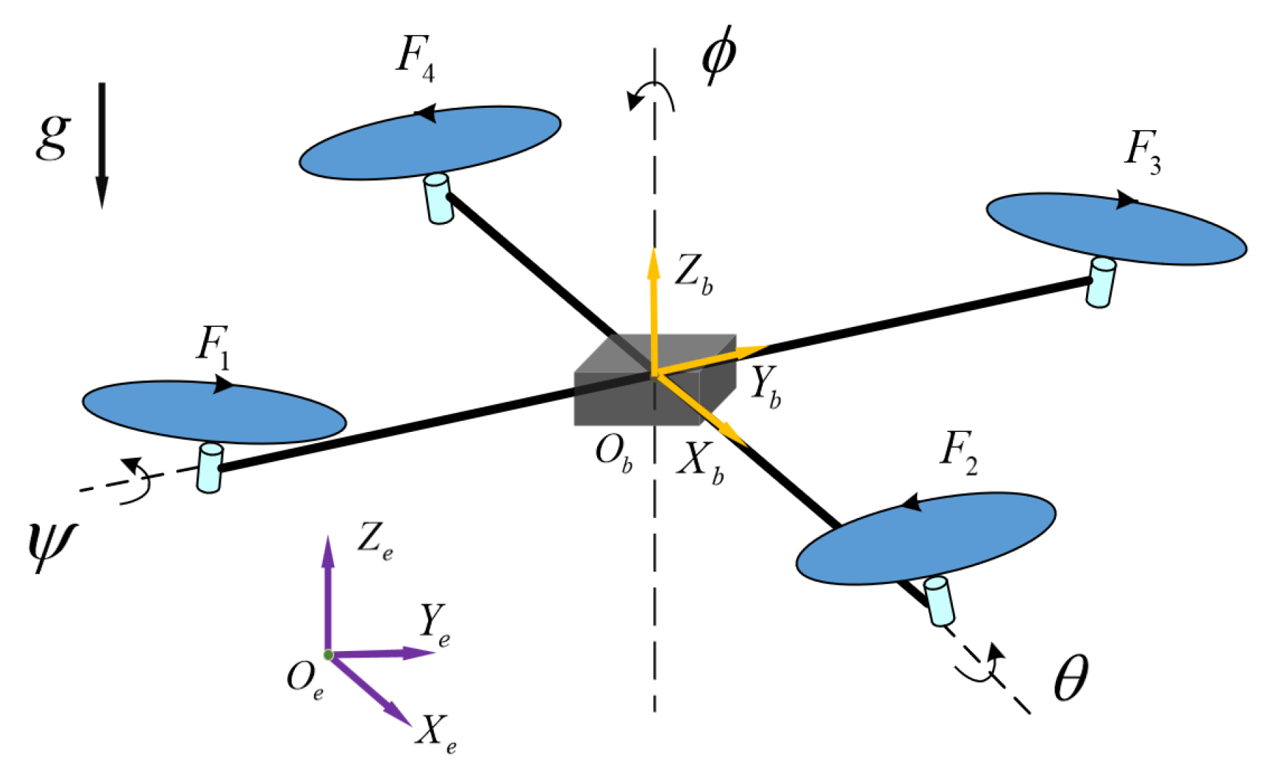
This paper considers a UAV swarm composed of quadrotor platforms. Although the proposed planning framework is developed for quadrotors, the same idea can be extended to other rotorcraft systems with similar translational motion characteristics. For the i-th UAV, its motion is described with respect to an Earth-fixed frame and a body-fixed frame, as illustrated in Figure 1. The Earth-fixed frame is denoted by $E=\left[X_e{Y}_e{Z}_e\right]$, where the $Z_e$-axis points upward. The body-fixed frame of the i-th UAV is denoted by $B_i=\left[X_{b,i}{Y}_{b,i}{Z}_{b,i}\right]$ and is attached to its center of mass, $i\in \mathcal{Q}=\left\{1,2,\dots ,N_{\mathrm{UAV}}\right\}$ and $N_{\mathrm{UAV}}$ is the number of cooperative UAVs. The origins of the inertial and body-fixed frames are represented by $O_e$ and $O_{b,i}$, respectively. The gravitational acceleration is denoted by g, while the Euler angles ${\varphi }_i$, ${\theta }_i$, and ${\psi }_i$ characterize the attitude of the i-th UAV, representing the roll angle, pitch angle, and yaw angle, respectively.

For each quadrotor, the full dynamics can be separated into translational and rotational subsystems. Since the cooperative trajectory planning problem studied in this paper mainly concerns position evolution, only the translational subsystem is adopted for prediction and optimization. The translational dynamics of the i-th UAV are given by

$${\dot{\mathsf{\eta }}}_i=\left[\begin{array}{c}{v}_{i,x}\\ v_{i,y}\\ v_{i,z}\\ {\displaystyle \frac{T_{F,i}}{m_i}}\left(\cos {\varphi }_i\sin {\theta }_i\cos {\psi }_i+\sin {\varphi }_i\sin {\psi }_i\right)\\ {\displaystyle \frac{T_{F,i}}{m_i}}\left(\cos {\varphi }_i\sin {\theta }_i\sin {\psi }_i-\cos {\psi }_i\sin {\varphi }_i\right)\\ {\displaystyle \frac{T_{F,i}}{m_i}}\cos {\theta }_i\cos {\varphi }_i-g\end{array}\right]$$

(1)

where ${\mathsf{\eta }}_i={[{\mathit{p}}_i,{\mathit{v}}_i]}^{\top }$ denotes the translational state of the i-th UAV, with ${\mathit{p}}_i={[x_i,y_i,z_i]}^{\top }$ and ${\mathit{v}}_i={[v_{i,x},v_{i,y},v_{i,z}]}^{\top }$ representing its position and velocity, respectively. The control input is described in terms of translational acceleration, namely ${\mathit{a}}_i={\dot{\mathit{v}}}_i={[a_{i,x},a_{i,y},a_{i,z}]}^{\top }$.

In this paper, it is assumed that each UAV is equipped with a high-bandwidth inner-loop attitude controller. Therefore, the proposed distributed NMPC framework mainly focuses on the outer-loop trajectory-planning layer for position and velocity control, where the translational acceleration ${\mathit{a}}_i$ is treated as the decision variable. The reference attitude angles can be determined according to (1) and then transmitted to the inner-loop attitude controller. More specifically, the reference attitude angles ${\varphi }_c$ and ${\theta }_c$ can be calculated by [28]:

$$\begin{array}{c}{\varphi }_c=\arcsin \left({\displaystyle \frac{m{a}_{i,x}\sin \left(\psi \right)-m{a}_{i,y}\cos \left(\psi \right)}{\sqrt{m^2{a}_{i,x}^2+m^2{a}_{i,y}^2+m^2{\left(a_{i,z}+g\right)}^2}}}\right)\end{array}$$

(2)

$$\begin{array}{c}{\theta }_c=\arctan \left({\displaystyle \frac{m{a}_{i,x}\cos \left(\psi \right)+m{a}_{i,y}\sin \left(\psi \right)}{m{a}_{i,z}+mg}}\right)\end{array}$$

(3)

and the reference yaw angle ${\psi }_c$ can be specified in advance.

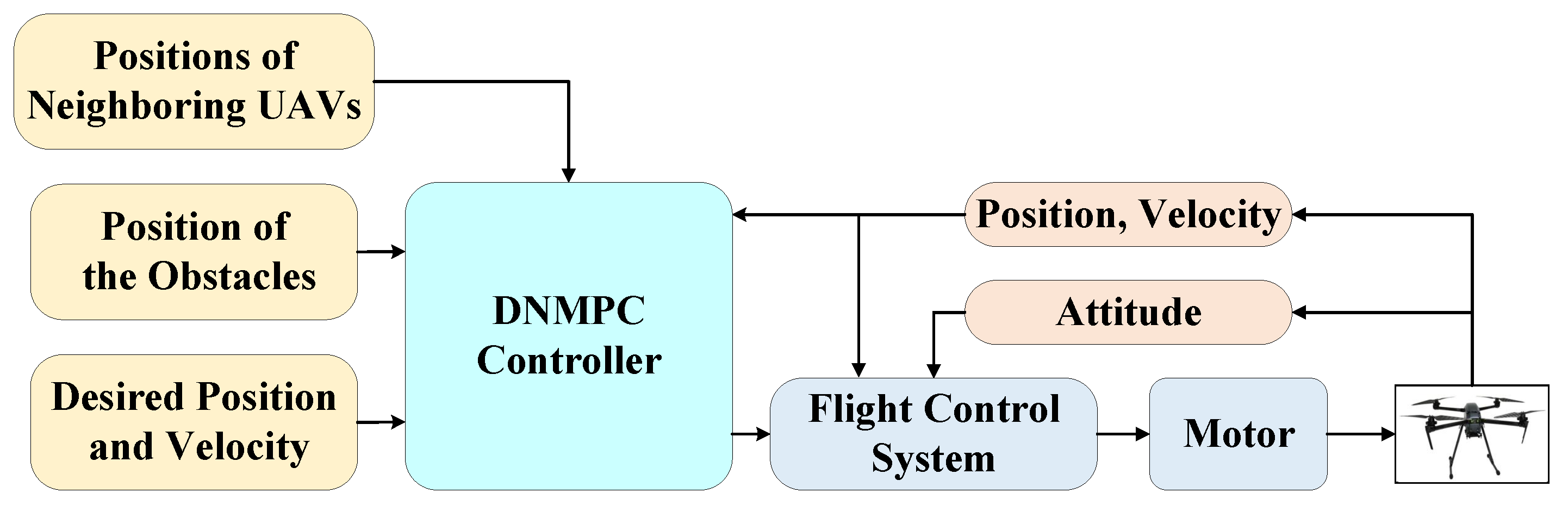
The control architecture of each UAV in the swarm is illustrated in Figure 2. At each sampling instant, the distributed NMPC module computes the optimal trajectory command online according to the current position and velocity of the i-th UAV, the desired target information, the obstacle position information, and the position information received from neighboring UAVs. The resulting reference command is then transmitted to the flight control system, which further generates the motor drive signals based on the measured attitude and motion states. In this way, each UAV can perform predictive planning while simultaneously achieving coordinated motion through neighbor information exchange.

2.2. Problem Statement

In this paper, the operational scenario considers a UAV swarm taking off from given initial positions, navigating around a set of obstacles, and eventually reaching their designated target points. The planning objectives are to minimize the overall flight cost while maintaining the desired formation during the maneuvering process. To guarantee flight safety and ensure physically feasible motion, constraints must first be imposed on the UAV dynamics.

2.2.1. Constraints

Due to the characteristics of the UAV, considering the physical limitations of the motor, we limit the velocity of the UAV. For each i-th UAV, the velocity constraint can be expressed in the following form

$${\mathit{v}}_{i,\min }\le {\mathit{v}}_i\left(\tau |t\right)\le {\mathit{v}}_{i,\max },\tau \in \left[t,t+T\right]$$

(4)

where ${\mathit{v}}_{i,\min }\in {\mathbb{R}}^3$ and ${\mathit{v}}_{i,\max }\in {\mathbb{R}}^3$, denote the minimum and maximum permissible velocities along the x, y, and z axes, respectively. Similarly, the acceleration of each UAV is constrained as follows

$${\mathit{a}}_{i,\min }\le {\mathit{a}}_i\left(\tau |t\right)\le {\mathit{a}}_{i,\max },\tau \in \left[t,t+T\right]$$

(5)

where ${\mathit{a}}_{i,\min }\in {\mathbb{R}}^3$ and ${\mathit{a}}_{i,\max }\in {\mathbb{R}}^3$, specify the lower and upper acceleration bounds. In addition to the dynamic constraints, collision avoidance constraints must be incorporated to ensure safe operation. Without loss of generality, cylindrical obstacles are considered as an example, and the obstacle avoidance constraint for the i-th UAV is formulated as

$$\parallel {\mathit{p}}_i\left(\tau |t\right)-{\mathsf{\xi }}_l\parallel \ge {\xi }_{lr},l=1,2,\dots ,N_{\mathrm{obs}}$$

(6)

where ${\mathsf{\xi }}_l$ and ${\xi }_{lr}$ represent the position and safety radius of the l-th obstacle, respectively, $l\in {\mathcal{Q}}_{\mathrm{obs}}=\left\{l=1,2,\dots ,N_{\mathrm{obs}}\right\}$ and $N_{\mathrm{obs}}$ is the number of obstacles. Accordingly, the obstacle-avoidance distance between UAV i and obstacle l is defined as

$${\rho }_{i,l}\left(t\right)=∥{\mathit{p}}_i\left(t\right)-{\mathsf{\xi }}_l∥,$$

(7)

which is used to evaluate whether the obstacle safety threshold ${\xi }_{lr}$ is satisfied.

Furthermore, each UAV i must maintain a safe distance from its neighboring UAV j to prevent collisions, $j\in \mathcal{Q}\setminus \left\{i\right\}$. Hence, the collision avoidance constraint between UAVs can be expressed as

$$\parallel {\mathit{p}}_i\left(\tau |t\right)-{\mathit{p}}_j\left(\tau |t\right)\parallel \ge {\xi }_{pr},j\in \mathcal{Q}\setminus \left\{i\right\}$$

(8)

where ${\xi }_{pr}$ represents the minimum permissible distance between any pair of UAVs. Accordingly, the inter-UAV distance between UAV i and UAV j is defined as

$${\xi }_{i,j}\left(t\right)=∥{\mathit{p}}_i\left(t\right)-{\mathit{p}}_j\left(t\right)∥,$$

(9)

which is used to evaluate whether the minimum inter-UAV safety distance ${\xi }_{pr}$ is maintained.

Remark 1. 

In practical obstacle avoidance scenarios, obstacles may also have conical, cuboid, or other irregular shapes. The corresponding obstacle avoidance constraints can generally be approximated or equivalently transformed into explicit nonlinear state constraints. Therefore, these obstacle models can also be readily incorporated into the proposed trajectory planning framework.

2.2.2. Objective Function

The model in (1) is used to predict the future trajectories of the UAV, and the prediction dynamics is written as

$${\dot{\mathsf{\eta }}}_i\left(\tau |t\right)={[{\mathit{v}}_i\left(\tau \right|t),{\mathit{a}}_i\left(\tau \right|t)]}^{\top },\tau \in \left[t,t+T\right]$$

where ${\mathsf{\eta }}_i\left(\tau |t\right)$ represents the predicted state for the i-th UAV at time $\tau$. This prediction is derived from its initial state at time t and the sequence of control inputs ${\mathit{a}}_i\left({\tau }^{\prime }|t\right)$ applied over the future time interval ${\tau }^{\prime }\in [t,\tau ]$, where T is the prediction horizon length. We define the state error as

$${\mathsf{\eta }}_{i,e}={\left[{{\mathit{p}}_{i,e}}^{\top },{{\mathit{v}}_{i,e}}^{\top }\right]}^{\top }$$

where ${\mathit{p}}_{i,e}={\mathit{p}}_i-{\mathit{p}}_{i,tgt}$ is the position error and ${\mathit{v}}_{i,e}={\mathit{v}}_i-{\mathit{v}}_{i,tgt}$ is the velocity error of the i-th UAV. Here, ${\mathit{p}}_{i,\mathrm{tgt}}\in {\mathbb{R}}^3$ denotes the reference position assigned to the i-th UAV in the target formation, and ${\mathit{v}}_{i,\mathrm{tgt}}\in {\mathbb{R}}^3$ denotes the corresponding desired velocity. The dynamics of the predicted state error ${\mathsf{\eta }}_{i,e}$ are then expressed as

$${\dot{\mathsf{\eta }}}_{i,e}\left(\tau |t\right)={[{\mathit{v}}_{i,e}\left(\tau \right|t),{\mathit{a}}_i\left(\tau \right|t)]}^{\top },\tau \in \left[t,t+T\right]$$

(10)

where ${\dot{\mathsf{\eta }}}_{i,e}$ can be easily obtained through translational subsystem (1). Furthermore, the UAV swarm is required to maintain a specific formation during flight. This formation is constructed based on the relative distances between UAVs, specified by the term ${∥{\mathit{p}}_i\left(\tau |t\right)-{\mathit{p}}_j\left(\tau |t\right)-{\mathsf{\theta }}_{ij}∥}^2$, where ${\mathsf{\theta }}_{ij}\in {\mathbb{R}}^3$ denotes the desired relative position vector of UAV i with respect to UAV j, $j\in \mathcal{Q}\setminus \left\{i\right\}$. Then, the objective function of UAV trajectory planning is defined as

$$J\left({\mathit{a}}_i\right)={\int }_t^{t+T}{\mathcal{L}}_i\left(\tau \right|t)\mathrm{d}\tau$$

(11)

where

$${\mathcal{L}}_i\left(\tau \right|t)={\beta }_1{∥{\mathsf{\eta }}_{i,e}\left(\tau \right|t)∥}^2+{\beta }_2\sum _{j\in \mathcal{Q}\setminus \left\{i\right\}}{∥{\mathit{p}}_i\left(\tau \right|t)-{\mathit{p}}_j\left(\tau \right|t)-{\mathsf{\theta }}_{ij}∥}^2+{\beta }_3{∥{\mathit{a}}_i\left(\tau \right|t)∥}^2$$

(12)

Here, ${\beta }_1$, ${\beta }_2$, and ${\beta }_3$ are weighting coefficients that balance the objectives of target reaching, formation maintenance, and acceleration oscillation suppression, respectively. The weighting coefficients ${\beta }_1$ and ${\beta }_2$ determine the trade-off between rapid target reaching and formation maintenance during flight. A larger ${\beta }_1$ places more emphasis on driving the UAVs toward the target positions as quickly as possible, whereas a larger ${\beta }_2$ prioritizes reducing the formation tracking error and preserving the desired geometric configuration during maneuvering.

Remark 2. 

It should be noted that the proposed framework is not restricted to a specific formation. By appropriately modifying the formation parameter θ, the proposed method can be extended to arbitrary 3D formation shapes, such as line-shaped, circular, and other customized formations.

2.2.3. Optimal Control Problem

The original UAV trajectory planning optimization problem, referred to as Problem P1, is formally stated as follows:

$$\begin{array}{cc}\hfill \underset{{\mathit{a}}_i\left(\tau \right|t),\tau \in \left[t,t+T\right]}{\min }& J\left({\mathit{a}}_i\right)\hfill \end{array}$$

(13a)

$$\begin{array}{cc}\hfill \mathrm{s}.\mathrm{t}.& {\dot{\mathsf{\eta }}}_i\left(\tau |t\right)={[{\mathit{v}}_i\left(\tau \right|t),{\mathit{a}}_i\left(\tau \right|t)]}^{\top },\tau \in \left[t,t+T\right]\hfill \end{array}$$

(13b)

$$\begin{array}{cc}\hfill & {\mathsf{\eta }}_i\left(t\right|t)={\mathsf{\eta }}_i\left(t\right)\hfill \end{array}$$

(13c)

$$\begin{array}{cc}\hfill & {\mathit{a}}_{i,\min }\le {\mathit{a}}_i\left(\tau |t\right)\le {\mathit{a}}_{i,\max },\tau \in \left[t,t+T\right]\hfill \end{array}$$

(13d)

$$\begin{array}{cc}\hfill & {\mathit{v}}_{i,\min }\le {\mathit{v}}_i\left(\tau |t\right)\le {\mathit{v}}_{i,\max },\tau \in \left[t,t+T\right]\hfill \end{array}$$

(13e)

$$\begin{array}{cc}\hfill & \parallel {\mathit{p}}_i\left(\tau |t\right)-{\mathsf{\xi }}_l\parallel \ge {\xi }_{lr},\tau \in [t,t+T],l\in {\mathcal{Q}}_{\mathrm{obs}}\hfill \end{array}$$

(13f)

$$\begin{array}{cc}\hfill & \parallel {\mathit{p}}_i\left(\tau |t\right)-{\mathit{p}}_j\left(\tau |t\right)\parallel \ge {\xi }_{pr},\tau \in [t,t+T],j\in \mathcal{Q}\setminus \left\{i\right\}\hfill \end{array}$$

(13g)

3. Proposed NMPC Algorithm

In this section, we develop an NMPC algorithm for cooperative trajectory planning of the UAV swarm. Within the proposed distributed NMPC framework, the original optimal control problem in (13) is transcribed into a finite-dimensional nonlinear programming problem by means of control parameterization.

To obtain an approximate solution, the prediction interval $[t,t+T]$ of each UAV is uniformly divided into M subintervals, and the control input is parameterized as follows. This treatment allows the continuous-time control problem to be represented by a finite number of decision variables, thereby improving computational efficiency for online implementation. Although such a discretization may introduce approximation error compared with the original continuous-time formulation, it avoids the repeated solution of differential equations with fully free control functions and is therefore more suitable for real-time trajectory generation in UAV swarm applications. For the i-th UAV, the control input ${\mathit{a}}_i$ is approximated by a piecewise-constant function ${\mathit{a}}_{i,p}$ according to [29]:

$${\mathit{a}}_{i,p}\left(\tau \right|t)={\displaystyle \sum _{k=1}^M}{\mathsf{\sigma }}_i^k{\chi }_i^k\left(\tau \right|t)$$

(14)

where ${\mathsf{\sigma }}_i^k={\left[{\sigma }_{i,1}^k,{\sigma }_{i,2}^k,{\sigma }_{i,3}^k\right]}^{\top }\in {\mathbb{R}}^3$, $k=1,2,\dots ,M$, denotes the parameter vector associated with the k-th control segment of the i-th UAV, and ${\chi }_i^k\left(\tau \right|t)$ is defined as

$$\begin{array}{c}{\chi }_i^k\left(\tau \right|t)=\left\{\begin{array}{cc}1,& \mathrm{if}\tau \in \left[t+{\displaystyle \frac{(k-1)T}{M}},t+{\displaystyle \frac{kT}{M}}\right)\\ 0,& \mathrm{otherwise}.\end{array}\right.\end{array}$$

(15)

According to the control parameterization in (14), the decision variables are now ${\mathsf{\sigma }}_i^k$, $k=1,2,\dots ,M$, and the total number of decision variables for each UAV is therefore $3M$.

Thus, the continuous control trajectory of each UAV over the prediction horizon is characterized by a finite set of control parameters, which significantly reduces the dimension of the online optimization variables and makes the distributed trajectory planning problem more tractable.

3.1. Constraints Handling Based on Exact Penalty Function

Furthermore, an exact penalty function method is employed to handle system constraints. With an appropriately chosen penalty parameter, this method ensures that the unconstrained optimization problem shares the same optimal solution as the original constrained problem. Consequently, the complex constrained optimization is transformed into a more efficient unconstrained solution process, significantly enhancing the computational efficiency of the algorithm.

Based on the exact penalty function method [30], the velocity constraint (13e) for the i-th UAV are transformed into the following form:

$$\begin{array}{cc}\hfill J_{i,v}=\sum _{m=1,2,3}{\omega }^{-\alpha }& (\max {\left\{0,{\left[{\mathit{v}}_i\right]}_m\left(\tau \right|t)-{\left[{\mathit{v}}_{i,\max }\right]}_m-{\omega }^{\gamma }W\right\}}^2\hfill \\ & +\max {\left\{0,{\left[{\mathit{v}}_{i,\min }\right]}_m\left(\tau \right|t)-{\left[{\mathit{v}}_i\right]}_m\left(\tau \right|t)-{\omega }^{\gamma }W\right\}}^2)\hfill \end{array}$$

(16)

where ${\left[\mathit{x}\right]}_i$ is the i-th element of a vector $\mathit{x}$, $\omega$ denotes a parameter that needs to be optimized. The terms $\alpha$, $\gamma$ and W are positive real-valued parameters satisfying $\alpha >1$ and $\gamma >2$. Herein, ${\omega }^{-\alpha }$ serves as the penalty weight, while ${\omega }^{\gamma }W$ acts as a relaxation factor, with W being the corresponding weighting coefficient for this factor.

Regarding the obstacle avoidance constraint for UAVs (13f), we propose an enhanced avoidance function based on the formulation in [31]. The obstacle avoidance cost $J_{i,l}^{\mathrm{obs}}$ is defined by a piecewise function that activates when the UAV enters the obstacle’s safety radius:

$$J_{i,l}^{\mathrm{obs}}=\left\{\begin{array}{cc}0,\hfill & \mathrm{if}{d}_{il}\left(\tau \right|t)\ge {\xi }_{lr}\hfill \\ J_{i,\mathrm{rep}}^{\mathrm{obs}}·J_{i,\mathrm{vel}}^{\mathrm{obs}},\hfill & \mathrm{if}{d}_{il}\left(\tau \right|t)<{\xi }_{lr}\hfill \end{array}\right.,l\in {\mathcal{Q}}_{\mathrm{obs}}$$

(17)

where $d_{il}\left(\tau \right|t)=\parallel {\mathit{p}}_i\left(\tau \right|t)-{\mathsf{\xi }}_l\parallel$ denotes the predicted Euclidean distance between the i-th UAV and l-th obstacle. The component $J_{i,\mathrm{rep}}^{\mathrm{obs}}$ represents the distance-based repulsive potential, formulated as

$$J_{i,\mathrm{rep}}^{\mathrm{obs}}={\displaystyle \frac{D}{\epsilon }}-{\displaystyle \frac{D}{{({\xi }_{lr}-d_{il}\left(\tau \right|t))}^3+\epsilon }}$$

(18)

where $D>0$ is the weighting coefficient determining the strength of the repulsive potential field, and $ϵ>0$ is a small positive constant introduced to avoid numerical singularity. The component $J_{i,\mathrm{vel}}^{\mathrm{obs}}$ is a velocity-dependent scaling factor that incorporates the relative velocity:

$$J_{i,\mathrm{vel}}^{\mathrm{obs}}=1+\lambda ·\max \left(0,{\mathit{v}}_i^{\top }{\mathit{n}}_{i,l}\right)$$

(19)

where ${\mathit{n}}_{i,l}$ is the unit vector pointing from the l-th obstacle to the i-th UAV, and $\lambda$ is a weighting parameter.

To ensure not only obstacle avoidance but also safe separation among UAVs, the inter-UAV collision avoidance constraint (8) is treated in the same penalty framework. Specifically, for each neighboring pair $(i,j)$, we define the separation function

$$g_{ij}\left(\tau \right|t)={\xi }_{pr}-∥{\mathit{p}}_i\left(\tau \right|t)-{\mathit{p}}_j\left(\tau \right|t)∥$$

(20)

Accordingly, the collision-avoidance penalty is constructed as

$$J_{i,\mathrm{col}}=\sum _{j\in \mathcal{Q}\setminus \left\{i\right\}}{\omega }^{-\alpha }{\left(\max \left\{0,g_{ij}\left(\tau \right|t)-{\omega }^{\gamma }W\right\}\right)}^2$$

(21)

This penalty term is activated only when the safety distance is violated (up to the relaxation margin ${\omega }^{\gamma }W$), and becomes zero otherwise.

3.2. Transformed Optimization Problem

By incorporating the penalty terms (16), (17), and (21) into the original objective (11), the constrained problem (13) is converted into an unconstrained optimization problem. Accordingly, the penalized cost functional associated with the i-th UAV is given by

$${\widehat{\mathcal{L}}}_i\left(\tau \right|t)={\mathcal{L}}_i\left(\tau \right|t)+J_{i,v}+\sum _{l\in {\mathcal{Q}}_{\mathrm{obs}}}{J}_{i,l}^{\mathrm{obs}}+\sum _{j\in \mathcal{Q}\setminus \left\{i\right\}}{J}_{i,\mathrm{col}}$$

(22)

where ${\mathcal{N}}_i$ denotes the set of neighboring UAVs involved in collision avoidance and formation maintenance. Based on (14), the decision variables become the control parameters ${\left\{{\mathsf{\sigma }}_i^k\right\}}_{k=1}^M$ for each UAV. Let ${\mathsf{\sigma }}_i={\left[{\left({\mathsf{\sigma }}_i^1\right)}^{\top },{\left({\mathsf{\sigma }}_i^2\right)}^{\top },\dots ,{\left({\mathsf{\sigma }}_i^M\right)}^{\top }\right]}^{\top }$. Then, the resulting trajectory planning Problem P2 for the i-th UAV, $i\in \mathcal{Q}$, is formulated as

$$\begin{array}{cc}\hfill \underset{{\mathsf{\sigma }}_i,\omega }{\min }& {\int }_t^{t+T}{\widehat{\mathcal{L}}}_i\left(\tau \right|t)\mathrm{d}\tau +\delta {\omega }^{\beta }\hfill \end{array}$$

(23a)

$$\begin{array}{cc}\hfill \mathrm{s}.\mathrm{t}.& {\dot{\mathsf{\eta }}}_i\left(\tau |t\right)={[{\mathit{v}}_i\left(\tau \right|t),{\mathit{a}}_{i,p}\left(\tau \right|t)]}^{\top },\tau \in [t,t+T]\hfill \end{array}$$

(23b)

$$\begin{array}{cc}\hfill & {\mathsf{\eta }}_i\left(t\right|t)={\mathsf{\eta }}_i\left(t\right)\hfill \end{array}$$

(23c)

$$\begin{array}{cc}\hfill & {\mathit{a}}_{i,p}\left(\tau \right|t)={\displaystyle \sum _{k=1}^M}{\mathsf{\sigma }}_i^k{\chi }_i^k\left(\tau \right|t),\tau \in [t,t+T]\hfill \end{array}$$

(23d)

$$\begin{array}{cc}\hfill & {\mathit{a}}_{i,\min }\le {\mathsf{\sigma }}_i^k\le {\mathit{a}}_{i,\max },k=1,2,\dots ,M\hfill \end{array}$$

(23e)

where $\delta$ is a large penalty coefficient and $\beta >2$ is a prescribed constant. During the optimization process, the term $\delta {\omega }^{\beta }$ drives $\omega$ toward smaller values. Consequently, the penalty weight ${\omega }^{-\alpha }$ in ${\widehat{\mathcal{L}}}_i$ increases, thereby encouraging constraint satisfaction while minimizing the original objective function ${\mathcal{L}}_i$. Terminal costs and constraints are commonly used in distributed MPC to establish recursive feasibility and closed-loop stability [32]. However, the control parameterization and exact penalty function introduced in Problem P2 make the construction of an appropriate terminal set difficult. Lyapunov-based MPC [33] may provide an alternative approach for establishing these properties and will be investigated in future work.

For completeness, using the previously defined prediction length N, the corresponding numerical integration nodes are given by ${\tau }_q=t+qT/N$, $q=0,1,\dots ,N$. Using the parameterized control input ${\mathit{a}}_{i,p}\left(\tau \right|t)={\sum }_{k=1}^M{\mathsf{\sigma }}_i^k{\chi }_i^k\left(\tau \right|t)$, the complete finite-dimensional NLP is summarized as

$$\begin{array}{cc}\hfill \underset{{\mathsf{\sigma }}_i,\omega }{\min }& {\displaystyle \frac{T}{N}}{\displaystyle \sum _{q=0}^{N-1}}{\widehat{\mathcal{L}}}_i\left({\tau }_q\right|t)+\delta {\omega }^{\beta }\hfill \\ \hfill \mathrm{s}.\mathrm{t}.& {\mathsf{\eta }}_i\left({\tau }_0\right|t)={\mathsf{\eta }}_i\left(t\right)\hfill \\ & {\mathsf{\eta }}_i\left({\tau }_{q+1}\right|t)={\mathsf{\eta }}_i\left({\tau }_q\right|t)+{\displaystyle \frac{T}{N}}{\left[{\mathit{v}}_i\left({\tau }_q\right|t),{\mathit{a}}_{i,p}\left({\tau }_q\right|t)\right]}^{\top },q=0,1,\dots ,N-1\hfill \\ & {\mathit{a}}_{i,\min }\le {\mathsf{\sigma }}_i^k\le {\mathit{a}}_{i,\max },k=1,2,\dots ,M\hfill \\ & \omega >0\hfill \end{array}$$

At each communication update, the neighboring trajectories in ${\widehat{\mathcal{L}}}_i\left({\tau }_q\right|t)$ satisfy ${\mathit{p}}_j\left({\tau }_q\right|t)={\widehat{\mathit{p}}}_j\left({\tau }_q\right|t)$ and are treated as fixed parameters. The velocity, obstacle-avoidance, and inter-UAV separation requirements are incorporated through the penalty terms defined above.

The resulting NLP (23) is solved at each sampling instant within the receding-horizon NMPC framework, and can be efficiently handled by mature nonlinear programming solvers, such as CasADi [34].

For problem (23), Algorithm 1 summarizes the distributed NMPC-based cooperative trajectory planning procedure for the UAV swarm governed by (1). In the distributed implementation, ${\mathit{p}}_i\left(\tau \right|t)$ is treated as the local decision variable of the i-th UAV decided by ${\mathit{a}}_i\left(\tau \right|t)$, while ${\mathit{p}}_j\left(\tau \right|t)$ denotes the predicted trajectory information received from neighboring UAVs according to the latest communication update. Since the future actual value of ${\mathit{p}}_j\left(\tau \right|t)$ cannot be exactly known at the current sampling instant, the trajectory optimality of the following DMPC may be slightly degraded compared with the centralized framework. However, the real-time planning capability of each UAV can be preserved, and the optimality degradation can be reduced by decreasing the control update interval $\Delta$.

Remark 3. 

For the initial shifted control sequence ${\widehat{\mathit{a}}}_i\left(\tau \right|t)$, $t=0$, an initial predicted trajectory can be generated by solving a centralized optimization problem during the initialization stage. Alternatively, ${\widehat{\mathit{a}}}_i\left(\tau \right|t)$ can be selected as a constant acceleration corresponding to hovering or straight line flight of the UAV.

Remark 4. 

If the NLP problem (23) becomes infeasible during online implementation, a feasible backup trajectory can still be generated by using conventional obstacle avoidance methods, such as artificial potential field based method, to ensure safe flight and collision avoidance. In addition, the distributed NMPC framework adopts a sequential update scheme. Specifically, after the optimal translational acceleration command ${\mathit{a}}_i\left(\tau \right|t)$ is obtained for the i-th UAV, the corresponding reference attitude angles are computed and transmitted to the inner-loop controller.

We now discuss the feasibility and convergence properties of the approximate control sequence obtained from problem (23). The following lemma shows that, under the neighboring information available at the current sampling instant, any feasible solution of the discretized penalized problem (23) preserves the feasibility of the original constrained problem (13) for each UAV.

Lemma 1. 

For any $\omega >0$, there exists a ${\gamma }_{\omega }>0$ such that for all $\gamma \in (0,{\gamma }_{\omega })$, if the i-th UAV obtains a control parameter vector ${\tilde{\mathsf{\sigma }}}_i$ by solving problem (23), then the corresponding piecewise-constant control input

$${\tilde{\mathit{a}}}_{i,p}\left(\tau \right|t)={\displaystyle \sum _{k=1}^M}{\tilde{\mathsf{\sigma }}}_i^k{\chi }_i^k\left(\tau \right|t),\tau \in [t,t+T]$$

when applied to system (1), satisfies the constraints (13a)–(13g) associated with the i-th UAV in the original problem, i.e.,

$$\begin{array}{c}{\mathit{a}}_{i,\min }\le {\tilde{\mathit{a}}}_{i,p}\left(\tau \right|t)\le {\mathit{a}}_{i,\max },{\mathit{v}}_{i,\min }\le {\mathit{v}}_i\left(\tau |t\right)\le {\mathit{v}}_{i,\max },\tau \in \left[t,t+T\right]\\ \parallel {\mathit{p}}_i\left(\tau |t\right)-{\mathsf{\xi }}_l\parallel \ge {\xi }_{lr},\tau \in [t,t+T],l\in {\mathcal{Q}}_{\mathrm{obs}}\\ \parallel {\mathit{p}}_i\left(\tau |t\right)-{\mathit{p}}_j\left(\tau |t\right)\parallel \ge {\xi }_{pr},\tau \in [t,t+T],j\in \mathcal{Q}\setminus \left\{i\right\}\end{array}$$

Algorithm 1 Distributed NMPC-Based Trajectory Planning Algorithm

Require:   1: The target positions ${\mathit{p}}_{i,\mathrm{tgt}}$, terminal velocities ${\mathit{v}}_{i,\mathrm{tgt}}$, obstacle positions ${\mathsf{\xi }}_l$ and safety radii ${\xi }_{lr}$, $l=1,2,\dots ,N_{\mathrm{obs}}$, minimum inter-UAV safety distance ${\xi }_{pr}$, desired relative position vectors ${\mathsf{\theta }}_{ij}$, prediction horizon length T, feedback parameter $\Delta \in (0,T]$, and the weighting and penalty parameters in (22). Online:   2: for  $t=0,\Delta ,2\Delta ,\dots$ do   3:     For the i-th UAV, sample the current state ${\mathsf{\eta }}_i\left(t\right)$ and exchange the following predicted trajectory ${\widehat{\mathit{p}}}_i\left(\tau \right|t)$, $\tau \in [t,t+T]$, with the neighboring UAVs $j\in \mathcal{Q}\setminus \left\{i\right\}$. Here, the trajectory ${\widehat{\mathit{p}}}_i\left(\tau \right|t)$ is generated using the shifted control sequence ${\widehat{\mathit{a}}}_i\left(\tau \right|t)$ constructed from the previously obtained optimal solution ${\mathit{a}}_i^{\ast }\left(\tau \right|t-\Delta )$, i.e., $${\widehat{\mathit{a}}}_i\left(\tau \right|t)=\left\{\begin{array}{cc}{\mathit{a}}_i^{\ast }\left(\tau \right|t-\Delta ),\hfill & \tau \in [t,t+T-\Delta ),\hfill \\ {\mathit{a}}_i^{\ast }(t+T-\Delta |t-\Delta ),\hfill & \tau \in [t+T-\Delta ,t+T].\end{array}\right.$$   4:     for $i=1,2,\dots ,N_{\mathrm{UAV}}$ in parallel do   5:        Set ${\mathsf{\eta }}_i\left(t\right|t)={\mathsf{\eta }}_i\left(t\right)$.   6:        Set ${\mathit{p}}_j\left(\tau \right|t)={\widehat{\mathit{p}}}_j\left(\tau \right|t)$, $j\in \mathcal{Q}\setminus \left\{i\right\}$, and solve the finite-dimensional optimization problem (23) associated with the i-th UAV to obtain the following optimal vector: $${\mathsf{\sigma }}_i^{\ast }={\left[{\left({\mathsf{\sigma }}_i^{\ast ,1}\right)}^{\top },{\left({\mathsf{\sigma }}_i^{\ast ,2}\right)}^{\top },\dots ,{\left({\mathsf{\sigma }}_i^{\ast ,M}\right)}^{\top }\right]}^{\top }$$   7:        Construct the predicted control input $${\mathit{a}}_i\left(\tau \right|t)={\displaystyle \sum _{k=1}^M}{\mathsf{\sigma }}_i^{\ast ,k}{\chi }_i^k\left(\tau \right|t),\tau \in [t,t+T].$$   8:        Compute the corresponding reference attitude angle commands from ${\mathit{a}}_i\left(\tau \right|t)$ according to (2), and transmit them to the inner-loop controller over the interval $[t,t+\Delta ]$.   9:     end for 10: end for

The following lemma establishes the convergence relationship between the optimal solution of the discretized penalized problem (23) and that of the original problem (13) for the optimization problem of each UAV.

Lemma 2. 

Let ${\mathsf{\sigma }}_i^{\ast }$ be an optimal solution to problem (23) for the i-th UAV, with ω and γ chosen according to Lemma 1. Suppose that the original problem (13) admits an optimal solution ${\mathit{a}}_i^{\ast }\left(\tau \right|t)$, $\tau \in [t,t+T]$. Then, by first taking $\omega \to 0$ and subsequently letting $M\to \infty$, the approximate control sequence generated by the transformed problem converges to the optimal objective value of the original problem, i.e.,

$$\underset{\omega \to 0}{\lim }\underset{M\to \infty }{\lim }J\left({\mathit{a}}_{i,p}^{\ast }\right)=J\left({\mathit{a}}_i^{\ast }\right)$$

with ${\mathit{a}}_{i,p}^{\ast }\left(\tau \right|t)={\sum }_{k=1}^M{\mathsf{\sigma }}_i^{\ast ,k}{\chi }_i^k\left(\tau \right|t),\tau \in [t,t+T]$.

Lemma 1 and Lemma 2 can be proven by Lemma 9.2.1 and Theorems 9.2.1 and 9.2.2 of [29], respectively, and the proofs are omitted for brevity.

Remark 5. 

Conventional stagewise MPC yields $3N$ control variables and N dependent path constraints [22,27]. Through control parameterization, the proposed method reduces the decision dimension to $3M+1$, while the exact penalty function incorporates the velocity and safety requirements into the objective; N is retained for numerical integration. More importantly, under the stated conditions, Lemma 1 establishes feasibility equivalence between Problems P1 and P2, whereas Lemma 2 proves convergence of the optimal objective value of Problem P2 to that of Problem P1.

4. Experiments and Discussion

4.1. Simulation Experiments

All simulations were conducted on a personal computer running Windows 11, equipped with a 12th Gen Intel(R) Core(TM) i7-12700H processor (2.30 GHz) and 64.0 GB RAM. The proposed distributed trajectory planner was implemented in MATLAB R2022b.

In the considered scenario, three UAVs are required to travel toward their respective target positions while maintaining a prescribed triangular formation. During the flight, the swarm must avoid all obstacles in the environment, satisfy inter-UAV collision avoidance requirements, and preserve formation coherence under dynamic and control constraints. The initial states of three UAVs are specified as ${\mathsf{\eta }}_1\left(0\right)={[-0.04,-3.02,1,0,0,0]}^{\top }$, ${\mathsf{\eta }}_2\left(0\right)={[-0.84,-3.02,1,0,0,0]}^{\top }$, and ${\mathsf{\eta }}_3\left(0\right)={[0.76,-3.02,1,0,0,0]}^{\top }$, respectively. Their corresponding reference positions are given by ${\mathit{p}}_{1,\mathrm{tgt}}={[-0.04,2.42,1]}^{\top }$, ${\mathit{p}}_{2,\mathrm{tgt}}={[-0.84,2,1]}^{\top }$, and ${\mathit{p}}_{3,\mathrm{tgt}}={[0.76,2,1]}^{\top }$. The reference velocities ${\mathit{v}}_{i,tgt}$, $i=1,2,3$, are set to zero.

Six obstacles are placed in the environment with centers located at ${\left[-0.27,-1.53,1\right]}^{\top }$, ${\left[0.61,-0.89,1\right]}^{\top }$, ${\left[-1,-0.34,1\right]}^{\top }$, ${\left[0.06,0,1\right]}^{\top }$, ${\left[-1,1.45,1\right]}^{\top }$, and ${\left[0.52,1.45,1\right]}^{\top }$, respectively. For each $l\in {\mathcal{Q}}_{\mathrm{obs}}$, the obstacle safety radius is set to ${\xi }_{lr}=0.5$. The minimum inter-UAV safety distance is chosen as ${\xi }_{pr}=0.35$.

The desired formation is specified through relative position offsets among the three UAVs so that a triangular formation can be maintained during the flight. Accordingly, the desired relative offsets are given by

$$\begin{array}{c}{\mathsf{\theta }}_{12}={[0.8,0.42,0]}^{\top },{\mathsf{\theta }}_{13}={[-0.8,0.42,0]}^{\top },{\mathsf{\theta }}_{21}={[-0.8,-0.42,0]}^{\top }\\ {\mathsf{\theta }}_{23}={[-1.6,0,0]}^{\top },{\mathsf{\theta }}_{31}={[0.8,-0.42,0]}^{\top },{\mathsf{\theta }}_{32}={[1.6,0,0]}^{\top }\end{array}$$

The velocity constraints are given as $\left|{\left[{\mathit{v}}_i\right]}_m\right|\le 0.4$, for $i=1,2,3$ and $m=1,2,3$. For each $i=1,2,3$, the control inputs satisfy $\left|{\left[{\mathit{a}}_i\right]}_m\right|\le 0.5$ for $m=1,2$ and $\left|{\left[{\mathit{a}}_i\right]}_m\right|\le 0.1$ for $m=3$.

A receding horizon NMPC scheme is employed with prediction horizon $T=0.8\mathrm{s}$, length $N=20$, and $\Delta =0.04$. The weighting coefficients in the objective function are selected as ${\beta }_1=0.3$, ${\beta }_2=0.7$ and ${\beta }_3=0.01$. For the exact penalty formulation, the parameters are chosen as $\alpha =1.5$, $\gamma =3$, $W=0.3$, $\beta =3$, and $\delta ={10}^8$. For the obstacle avoidance term, the parameters are set to $ϵ=0.01$, $D=100$, and $\lambda =0.5$.

The closed-loop simulation terminates when all three UAVs move sufficiently close to their corresponding target positions, namely, $\parallel {\mathit{p}}_i-{\mathit{p}}_{i,\mathrm{tgt}}\parallel < 0.05,i=1,2,3.$

The simulation results are presented in Figure 3, Figure 4, Figure 5 and Figure 6 to evaluate the effectiveness of the proposed distributed NMPC framework for UAV swarm trajectory planning.

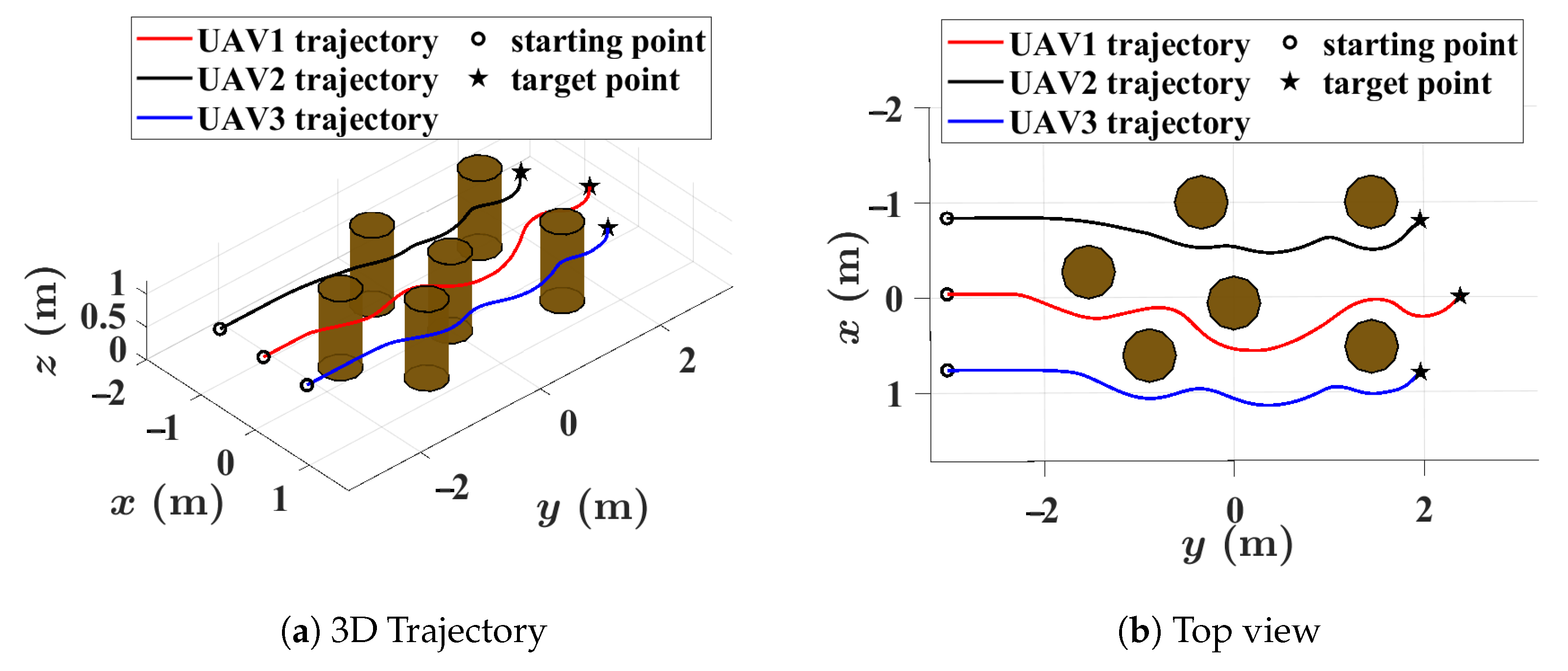
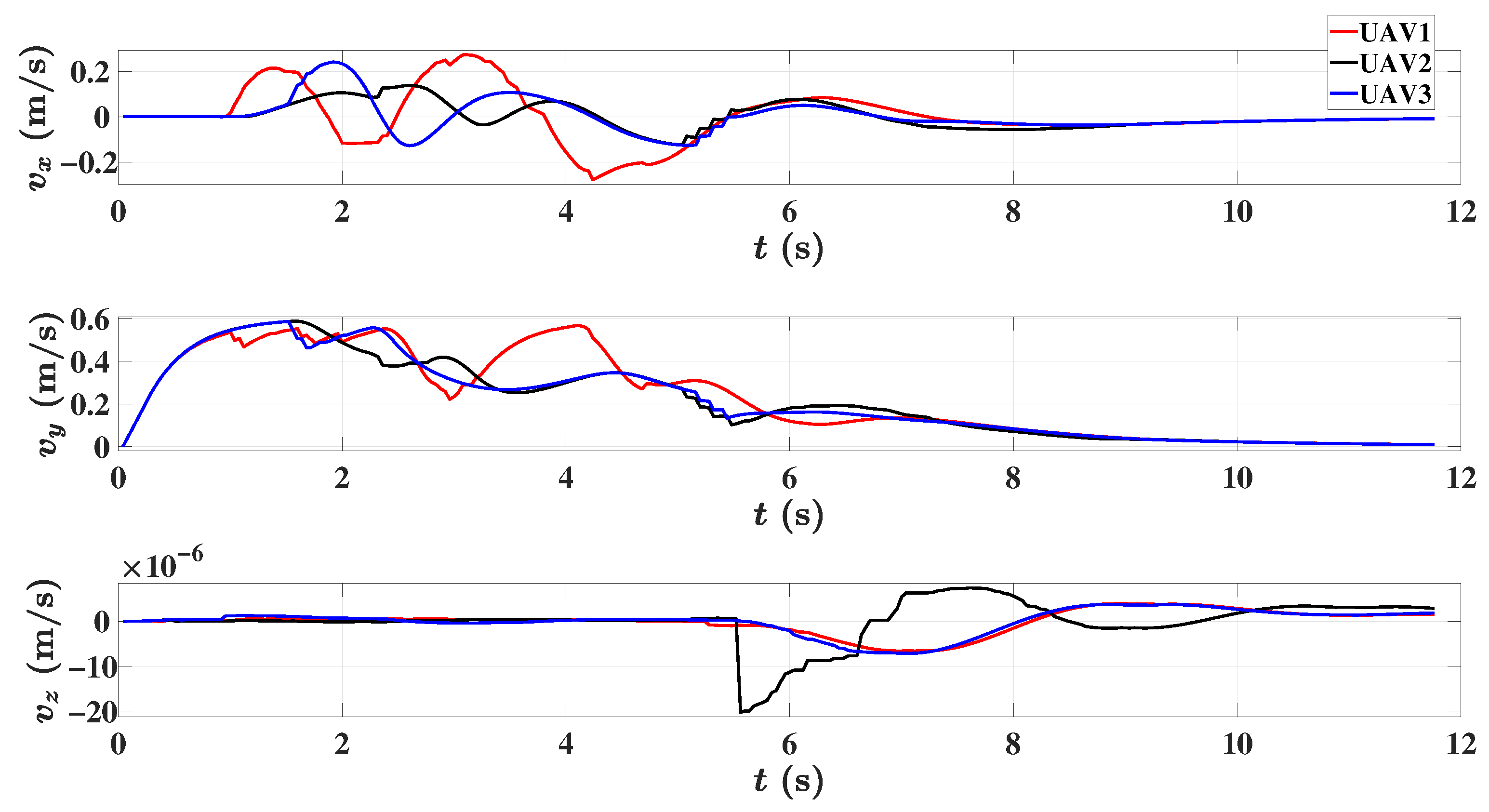
In the considered obstacle-rich environment, Figure 3 shows that the UAV swarm can safely avoid all obstacles and reach the prescribed target positions while maintaining the desired formation. Figure 4 depicts the velocity profiles of the three UAVs along the x-, y-, and z-axes. It is evident that the velocity components vary smoothly during the entire flight and remain within the prescribed bounds. In particular, the z-direction velocity remains close to zero, which is consistent with the mission setup in which the three UAVs mainly perform planar maneuvering at an approximately constant altitude. This result verifies that the proposed controller can generate dynamically feasible trajectories while respecting the velocity constraints.

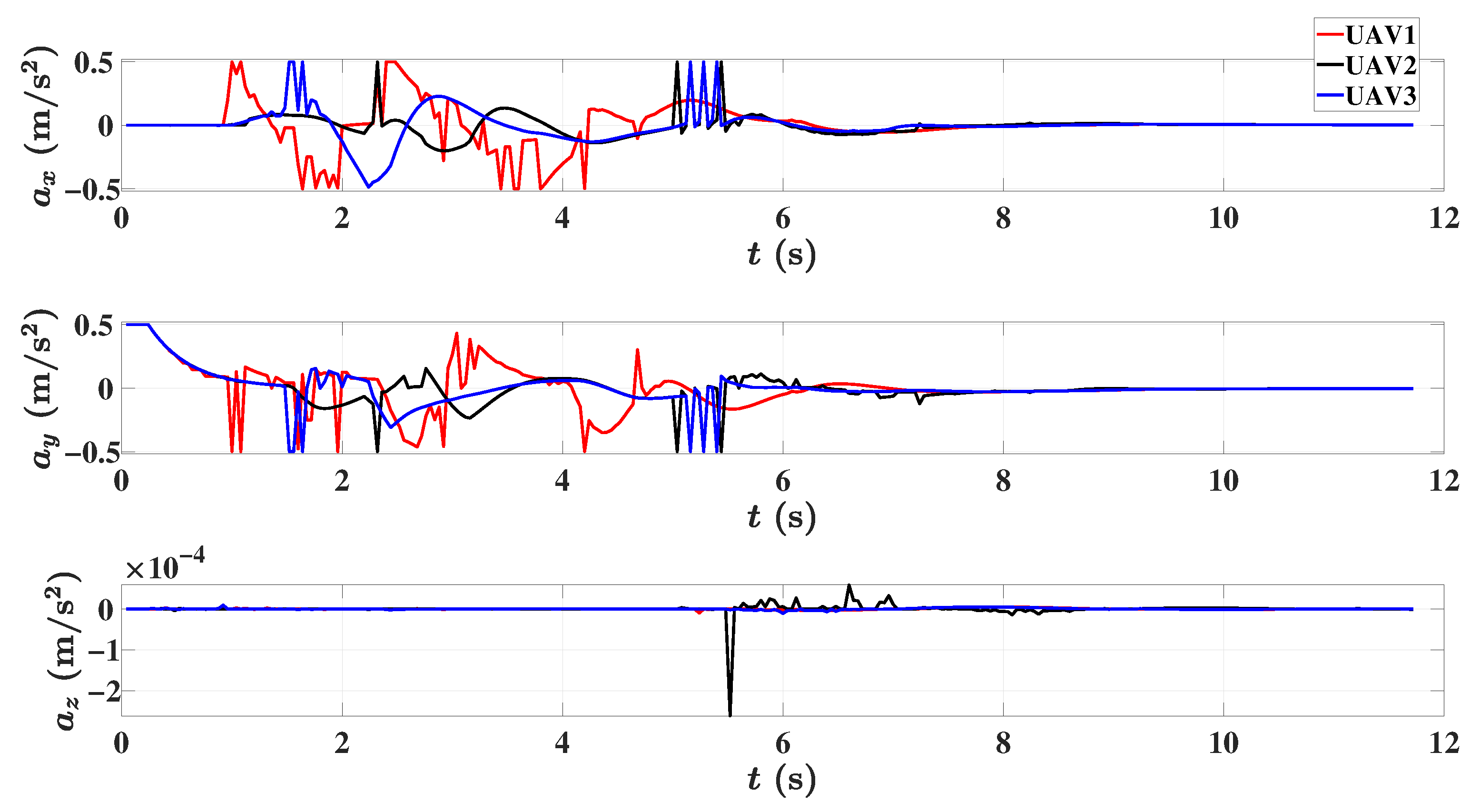
The corresponding acceleration commands are shown in Figure 5. The control inputs of all three UAVs remain bounded and evolve smoothly without aggressive oscillations. The accumulated control effort is ${\sum }_{i=1}^3{\int }_0^T{\parallel {\mathit{a}}_i\left(t\right)\parallel }^2\mathrm{d}t=1.27$. For clarity, the formation error between the i-th UAV and the j-th UAV is defined as

$$e_{i,j}\left(t\right)=∥\left({\mathit{p}}_i\left(t\right)-{\mathit{p}}_j\left(t\right)\right)-{\mathsf{\theta }}_{ij}∥.$$

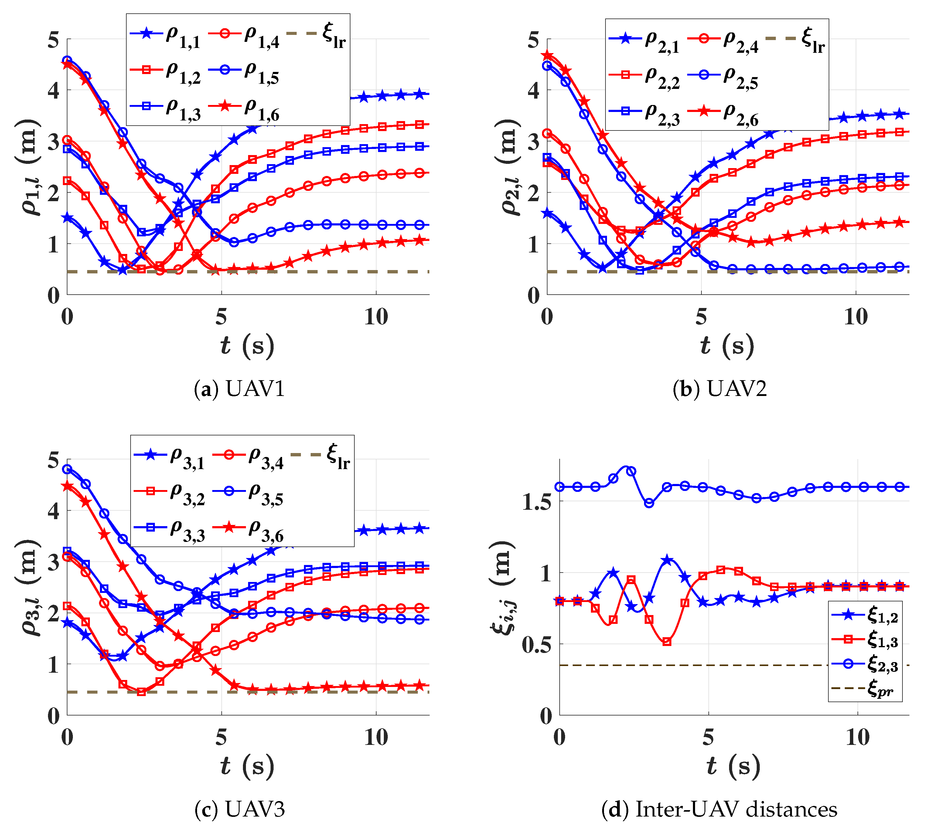
To further examine the obstacle avoidance and inter-UAV collision avoidance performance, Figure 6 presents the corresponding distance evolutions in simulation. For all three UAVs, the distances to surrounding obstacles and other UAVs remain above the prescribed safety threshold throughout the flight. More specifically, the minimum obstacle and inter-UAV distances are $0.5$ and $0.51$, respectively, both satisfying the thresholds of $0.5$ and $0.35$, thereby demonstrating that the proposed distributed planning method can successfully prevent inter-UAV collisions while maintaining the desired formation pattern.

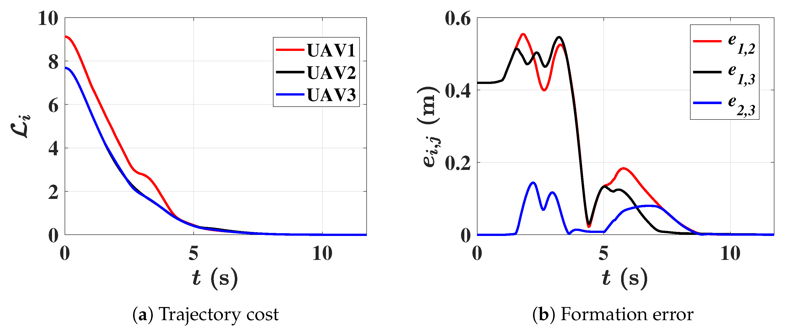
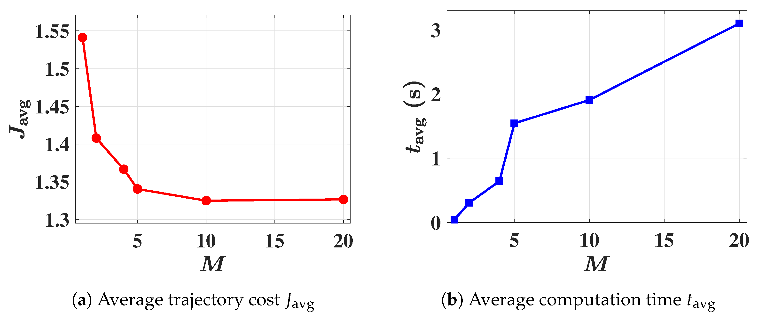
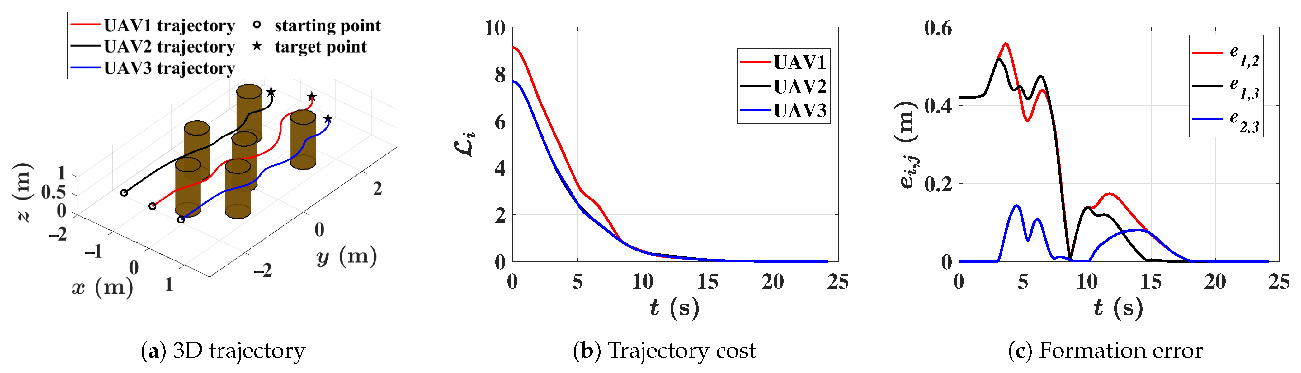
Figure 7 shows that the trajectory costs and formation errors gradually converge close to zero and the root mean square value of the formation error is $0.2292$, indicating that the proposed method can achieve target convergence while maintaining the desired formation within a certain formation error during obstacle avoidance and inter-UAV collision avoidance. In addition, Figure 8 shows that increasing M improves trajectory planning performance by reducing the average trajectory cost, although the improvement gradually becomes saturated. Meanwhile, the average computation time increases with M, indicating a higher online computational burden under finer control parameterization.

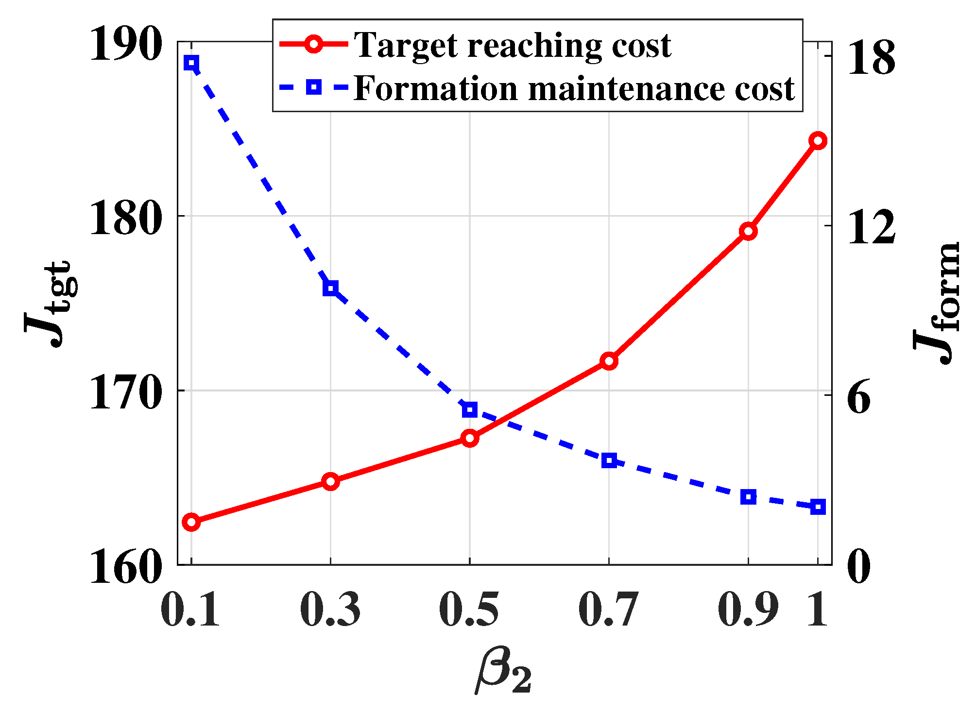
To provide a quantitative basis for the weighting selection, ${\beta }_1=0.3$ and ${\beta }_3=0.01$ are fixed. Since energy consumption, as reflected by the control-input term, is not the primary focus of this study, ${\beta }_3$ is assigned a relatively small value, and the analysis focuses on the two main objectives of target reaching and formation maintenance. To examine the influence of the formation maintenance weight, ${\beta }_2$ is set to $0.1$, $0.3$, $0.5$, $0.7$, $0.9$, and $1.0$ for comparison. Figure 9 presents the unweighted target reaching cost component $J_{\mathrm{tgt}}$ and formation-maintenance cost component $J_{\mathrm{form}}$ accumulated over the complete flights of the three UAVs. As ${\beta }_2$ increases, $J_{\mathrm{form}}$ decreases, whereas $J_{\mathrm{tgt}}$ increases. Based on these results, ${\beta }_1=0.3$ and ${\beta }_2=0.7$ are adopted so that both target reaching and formation maintenance are adequately considered in the objective function.

To further evaluate the effectiveness of the proposed framework,

Table 2. Comparison of different MPC-based methods.

	Average Trajectory Cost	Average Computation Time (s)	Computational Complexity
Proposed DNMPC	1.5411	0.0441	$\mathcal{O}\left({(4M+(N_{\mathrm{obs}}+3))}^3\right)$
Proposed CNMPC	1.4926	0.3761	$\mathcal{O}\left({(12M+3(N_{\mathrm{obs}}+3))}^3\right)$
NMPC [22]	1.2198	0.4470	$\mathcal{O}\left({(15N+4N_{\mathrm{nbr}})}^3\right)$

compares the proposed distributed NMPC (DNMPC) with its centralized counterpart, referred to as centralized NMPC (CNMPC), and the NMPC method in [22]. Here, the average trajectory cost denotes the mean accumulated trajectory cost over all UAVs during the closed-loop planning process, and a smaller value indicates better trajectory planning performance. The centralized NMPC achieves the lowest average trajectory cost by optimizing the trajectories of all three UAVs in a fully coupled manner. Although the proposed distributed NMPC yields a slightly higher trajectory cost, it significantly reduces the average computation time, demonstrating improved online computational efficiency. Compared with the NMPC method in [22], the proposed distributed NMPC also requires much less computation time. Although the NMPC method in [22] achieves better control performance, its significantly higher computational complexity makes real-time trajectory planning difficult, which is also reflected in the computational complexity results [27]. In contrast, the proposed distributed NMPC achieves a better trade-off between computational efficiency and control performance, enabling real-time trajectory planning while maintaining satisfactory control performance.

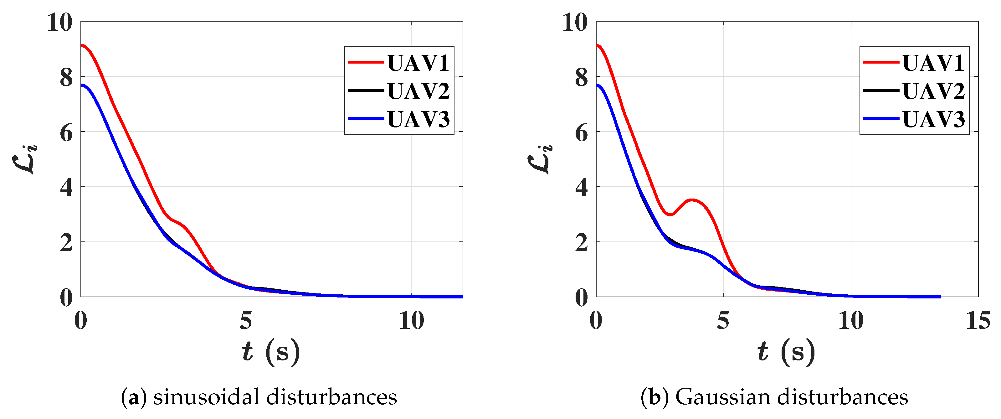
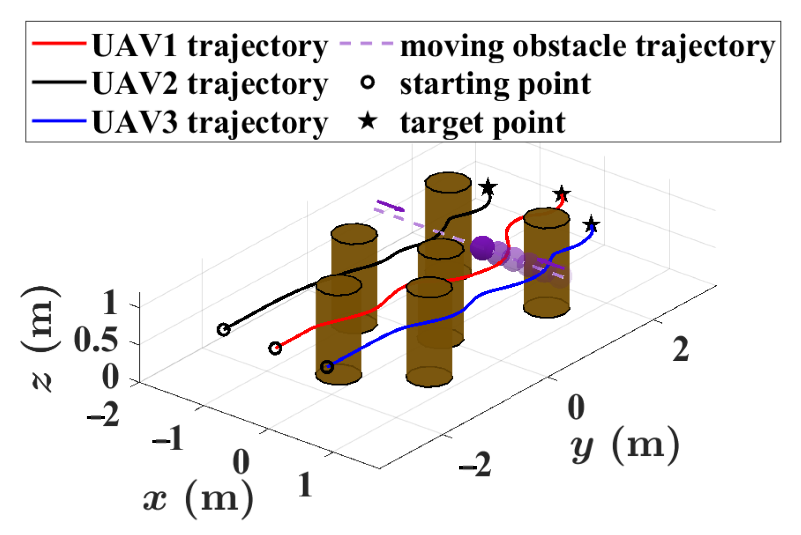
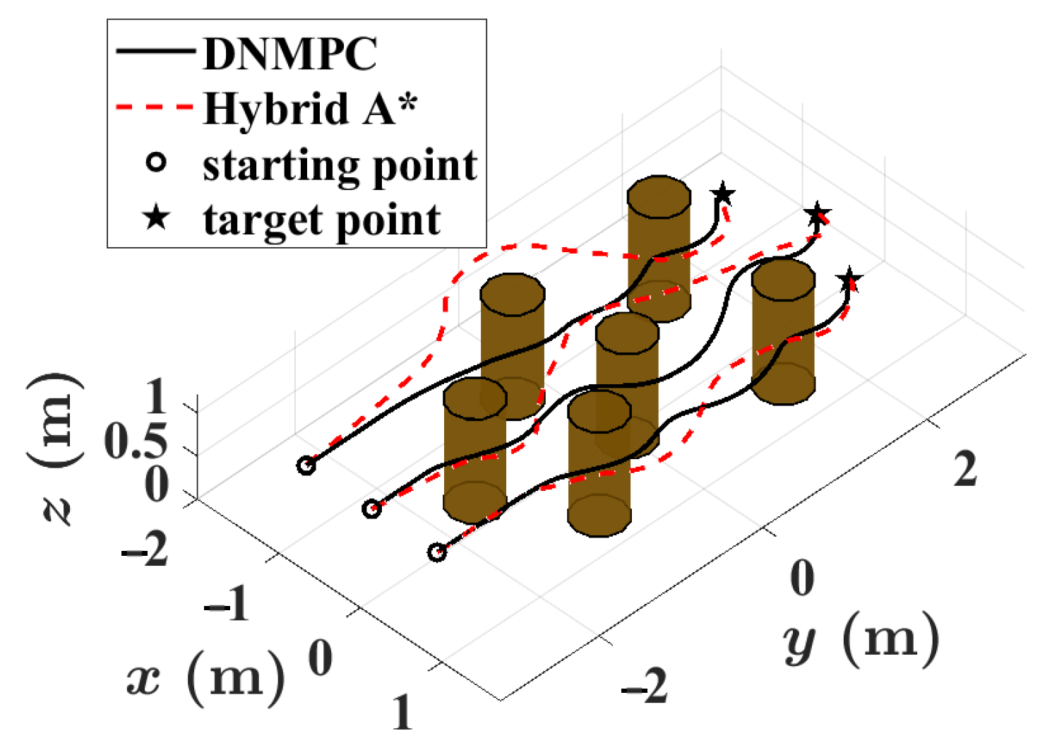
To assess the robustness of the proposed method, additional simulations are conducted under sinusoidal disturbances with an amplitude of ${10}^{-2}$ and Gaussian disturbances with variance ${10}^{-6}$ and range $\pm 3\times {10}^{-5}$. The results in Figure 10 show that the trajectory costs decrease and the formation errors converge close to zero. To further evaluate the dynamic-obstacle avoidance capability of the proposed method, a moving obstacle with a radius of $0.15\mathrm{m}$ is introduced, which moves back and forth at $0.5\mathrm{m}/\mathrm{s}$ along the x-direction within $x\in [-1.5,1.5]\mathrm{m}$, while maintaining $y=0.65\mathrm{m}$ and $z=1\mathrm{m}$. As shown in Figure 11, the three UAVs continuously update their planned trajectories to avoid the moving obstacle and reach the desired terminal formation without collision. This result demonstrates the capability of the proposed method to handle time-varying obstacle constraints in online multi UAV trajectory planning. Beyond the above evaluation in a dynamic environment, the competitiveness of the proposed method is further assessed through a planar comparison with Hybrid A* [35] in the same static obstacle scenario. Since the adopted Hybrid A* implementation performs planning in the horizontal plane, only the x-y trajectories of the two methods are considered to ensure a consistent comparison. As shown in Figure 12, both methods generate collision-free trajectories for the three UAVs. Hybrid A* achieves a shorter average single-step computation time of $0.02077\mathrm{s}$, compared with $0.04556\mathrm{s}$ for DNMPC. However, its average planar trajectory cost is $2.7984$, whereas that of DNMPC is only $1.5385$. These results indicate that the proposed DNMPC method achieves better trajectory quality according to the adopted cost criterion at the expense of a moderate increase in computation time.

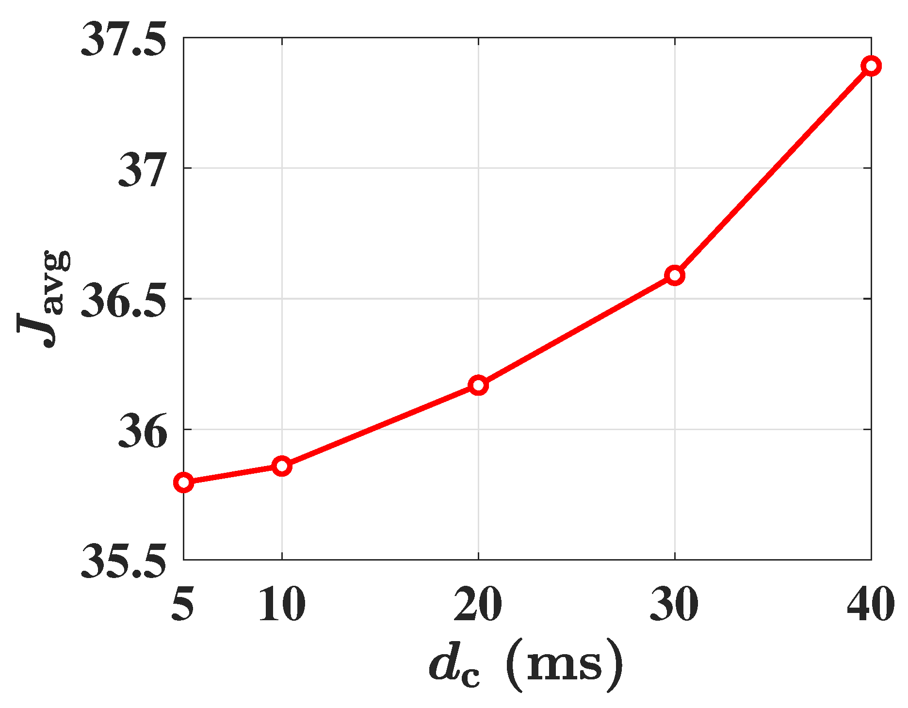
To evaluate the influence of nonideal communication, a fixed $10\mathrm{ms}$ delay is introduced into the neighbor-state information available to each UAV. As shown in Figure 13, the three UAVs satisfy the prescribed state and safety constraints and reach their assigned target positions, while the trajectory costs decrease and the formation errors converge close to zero. The maneuver duration is longer than that in the delay free case because the local planners use delayed neighbor information, which reduces the responsiveness of cooperative trajectory updates. To further quantify this influence, the communication delay $d_{\mathrm{c}}$ is varied from 5 to $40\mathrm{ms}$. As shown in Figure 14, the average trajectory cost exhibits an overall increasing trend with $d_{\mathrm{c}}$, indicating degraded trajectory planning performance under longer delays. Future work will investigate distributed MPC schemes [36] that explicitly incorporate delayed information from neighboring UAVs into the receding horizon optimization to mitigate this degradation.

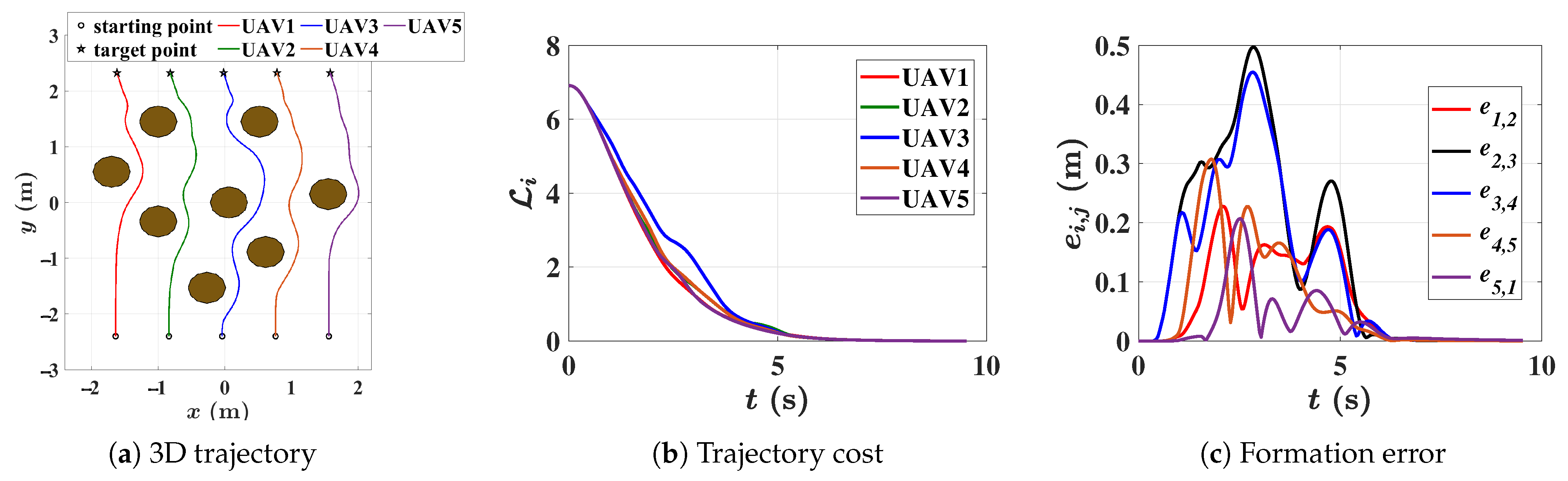
Furthermore, the simulation scenario is extended from three UAVs with a triangular formation to five UAVs with a line shaped formation. As shown in Figure 15a–c, the five UAVs can still safely reach the desired line shaped terminal formation, with decreasing trajectory costs and convergent formation errors. This result also shows that the proposed framework is not restricted to a specific formation pattern, since different formations can be specified by adjusting the desired relative position vectors. Moreover, the average single-step computation time of each UAV is about $0.0385\mathrm{s}$, which is close to that in the 3-UAV case. This indicates that the online computational burden of each UAV does not increase significantly when the swarm size increases from three to five, thereby verifying the scalability of the proposed method.

4.2. Flight Experiments

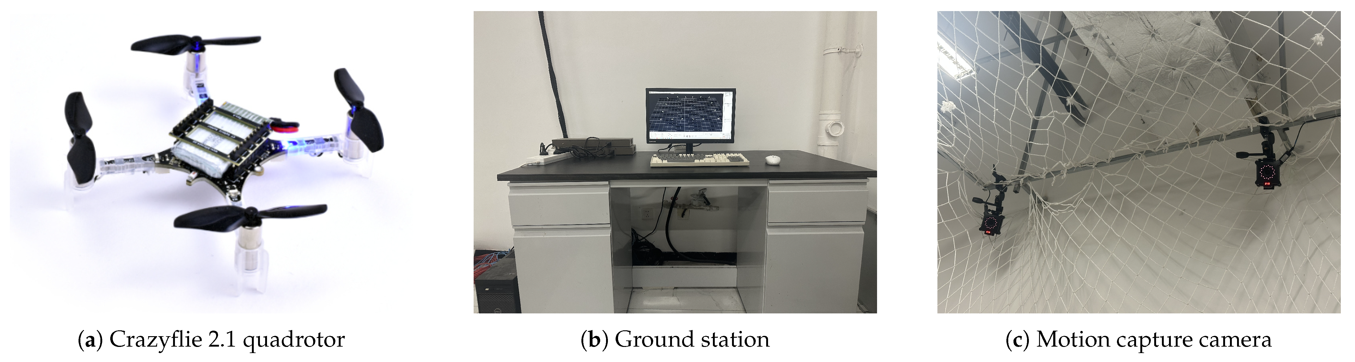
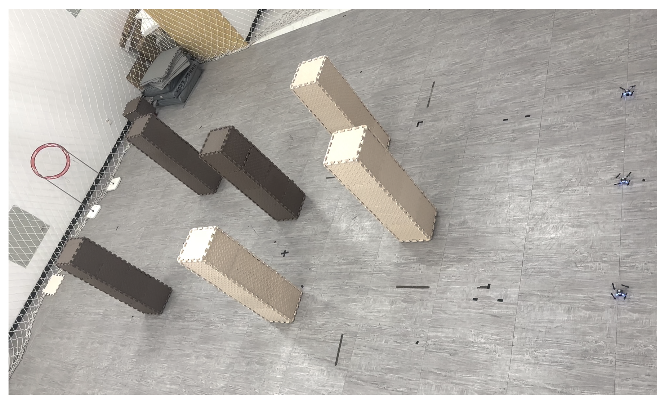
To further validate the practical applicability of the proposed distributed NMPC-based trajectory planning method, flight experiments were conducted using three Crazyflie 2.1 quadrotors. The main components of the experimental platform are shown in Figure 16, including the Crazyflie 2.1 quadrotor, the ground station, and the motion capture system. The flight experimental scenario is shown in Figure 17. The experimental system consists of three Crazyflie 2.1 quadrotors, a NOKOV motion capture system, a ground station, and a Crazyradio communication module.

During the experiment, the NOKOV motion capture system provides the position and velocity measurements of each UAV in the inertial frame. These real-time motion states are transmitted to the ground station, where the distributed NMPC optimization problems are solved online based on the current states of the UAVs. The generated reference commands are then sent to the corresponding Crazyflie quadrotors through Crazyradio. After receiving the commands, the onboard low-level controller of each Crazyflie tracks the reference commands to realize the planned motion. In this way, a closed-loop experimental system is established, where the proposed distributed NMPC algorithm generates online planning commands based on real-time feedback from the motion capture system. The ground station is equipped with an Intel(R) Core(TM) i7-10700 CPU at 2.90 GHz and 16 GB RAM. The experimental program is executed in an Ubuntu 20.04 environment running on a Windows 11 system, where IPOPT is used as the nonlinear programming solver and CppAD is used for automatic differentiation.

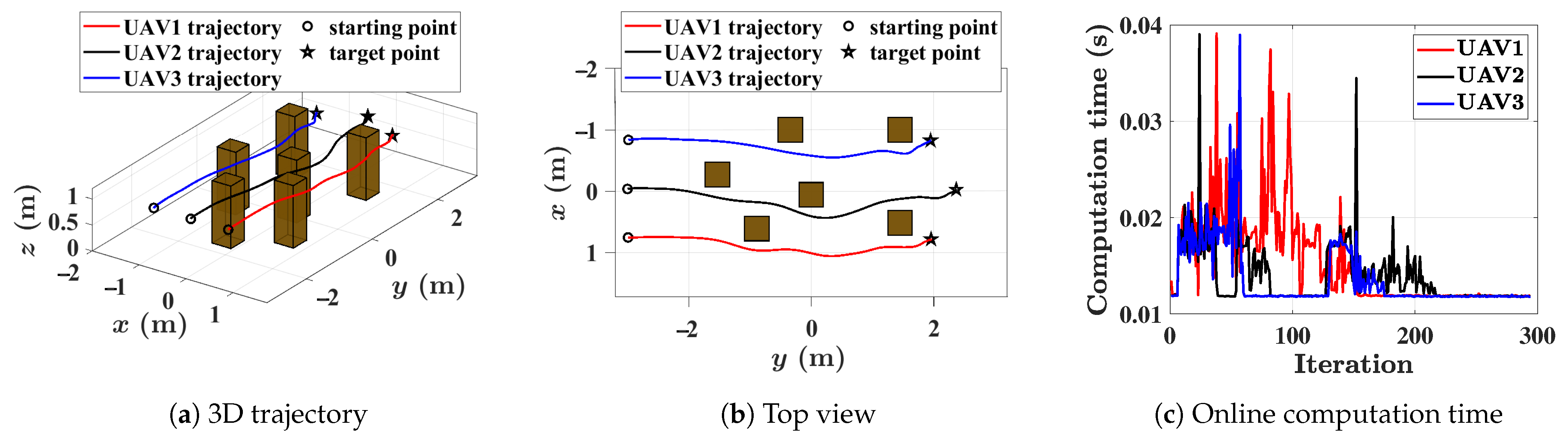
The flight experimental scenario is designed to be consistent with the three-UAV simulation scenario. The three UAVs are required to move from their initial positions to the assigned target positions while maintaining the desired formation and avoiding collisions with obstacles and other UAVs. Most of the NMPC parameters are kept the same as those used in the simulation. Different from the cylindrical obstacles used in the simulation, cuboid obstacles are adopted in the flight experiment. As discussed in Remark 1, non-circular or irregular obstacles can be approximated or equivalently transformed into explicit nonlinear state constraints. Therefore, in the flight experiment, each cuboid obstacle is conservatively represented by an inflated cylindrical safety region in the horizontal plane, so that the same obstacle-avoidance formulation can be used in the proposed NMPC framework. Considering the physical size of the Crazyflie platform, the tracking accuracy of the motion capture system, and the safety margin required in real flight, the obstacle safety radius and the inter-UAV safety radius are set to $0.4$ and $0.2$, respectively, in the flight experiment. Figure 18c shows the online computation time of the three UAVs at each control step. The corresponding average computation time and maximum single-step computation time are summarized in

Table 3. Online computation time of the proposed distributed NMPC method in the flight experiment.

	Average Computation Time (ms)	Maximum Computation Time (ms)
UAV 1	15.248	39.117
UAV 2	13.858	39.035
UAV 3	13.620	38.989

. The maximum single-step computation times of all UAVs are below $40\mathrm{ms}$. These results indicate that the proposed distributed NMPC method can be solved efficiently in the flight experiment and is suitable for online implementation on the experimental platform.

5. Conclusions

This paper investigates the cooperative trajectory planning problem for UAV swarms in obstacle-rich environments. A distributed nonlinear model predictive control framework was developed to address terminal target reaching, formation maintenance, obstacle avoidance, and inter-UAV collision avoidance in a unified manner. By combining control parameterization with exact-penalty-based constraint handling, the original constrained optimal control problem was transformed into a lower-complexity finite-dimensional NLP problem, which is more suitable for online implementation. Simulation and experimental results show that the proposed method can generate dynamically feasible and collision-free trajectories for multi-UAV systems, while the velocity and acceleration remain within the prescribed bounds. A limitation of the present formulation is that it employs only a stage cost without introducing a terminal cost. Therefore, recursive feasibility, closed-loop stability, and asymptotic convergence have not been theoretically established in this work. Future work will investigate distributed MPC frameworks with rigorous theoretical guarantees, dynamic-obstacle environments involving online motion estimation and prediction under uncertainty, and communication-aware distributed planning under bandwidth limitations, communication delays, and packet loss.

References

1. Vásárhelyi, G.; Virágh, C.; Somorjai, G.; Nepusz, T.; Eiben, A.E.; Vicsek, T. Optimized flocking of autonomous drones in confined environments. Sci. Robot. 2018, 3, eaat3536. [Google Scholar] [CrossRef] [Scilit] [PubMed]
2. Zhou, X.; Wen, X.; Wang, Z.; Gao, Y.; Li, H.; Wang, Q.; Yang, T.; Lu, H.; Cao, Y.; Xu, C.; et al. Swarm of micro flying robots in the wild. Sci. Robot. 2022, 7, eabm5954. [Google Scholar] [CrossRef] [Scilit] [PubMed]
3. Ren, Y.; Zhu, F.; Lu, G.; Cai, Y.; Yin, L.; Kong, F.; Lin, J.; Chen, N.; Zhang, F. Safety-assured high-speed navigation for MAVs. Sci. Robot. 2025, 10, eado6187. [Google Scholar] [CrossRef] [Scilit] [PubMed]
4. Javed, S.; Hassan, A.; Ahmad, R.; Ahmed, W.; Ahmed, R.; Saadat, A.; Guizani, M. State-of-the-Art and Future Research Challenges in UAV Swarms. IEEE Internet Things J. 2024, 11, 19023–19045. [Google Scholar] [CrossRef] [Scilit]
5. Xiao, R.; Wang, S.; Xie, Y.; Zhang, Y.; Xie, S.Q. Safety-Aware UAV Formation Scheme for Guiding UGVs Through Obstacle-Laden Environments. IEEE Robot. Autom. Lett. 2025, 10, 6999–7006. [Google Scholar] [CrossRef] [Scilit]
6. Cheng, Z.; Yang, J.; Sun, J.; Zhao, L. Trajectory Planning of Unmanned Aerial Vehicles in Complex Environments Based on Intelligent Algorithm. Drones 2025, 9, 468. [Google Scholar] [CrossRef] [Scilit]
7. Fan, X.; Li, H.; Chen, Y.; Dong, D. UAV Swarm Search Path Planning Method Based on Probability of Containment. Drones 2024, 8, 132. [Google Scholar] [CrossRef] [Scilit]
8. Yuan, W.; Chen, S.; He, H.; Hou, Y.; Chen, S.; Tan, X.; Yang, J. Hierarchical Reinforcement Learning-Based Joint Trajectory Planning and Resource Allocation in UAV-Assisted IoT-Sensor Networks. IEEE Trans. Commun. 2025, 73, 14517–14533. [Google Scholar] [CrossRef] [Scilit]
9. Khargharia, H.S.; Ouali, A.; Shakya, S.; Ahmad, S. Collision Avoidance in UAV Swarms: A Learning-Centric Perspective on Collaborative Intelligence. Neurocomputing 2026, 663, 132020. [Google Scholar] [CrossRef] [Scilit]
10. Sun, H.; Chen, H.; Ni, Z.; Fan, X.; Li, G.; Xia, F. Computing While Navigating: A Novel Task Offloading and Trajectory Planning Scheme for UAV-Assisted MEC System. IEEE Trans. Veh. Technol. 2026, 75, 3149–3159. [Google Scholar] [CrossRef] [Scilit]
11. Huang, S.; Zhang, H.; Huang, Z. E2CoPre: Energy Efficient and Cooperative Collision Avoidance for UAV Swarms with Trajectory Prediction. IEEE Trans. Intell. Transp. Syst. 2024, 25, 6951–6963. [Google Scholar] [CrossRef] [Scilit]
12. Huang, T.; Pan, H.; Sun, W.; Gao, H. Sine Resistance Network-Based Motion Planning Approach for Autonomous Electric Vehicles in Dynamic Environments. IEEE Trans. Transp. Electrif. 2022, 8, 2862–2873. [Google Scholar] [CrossRef] [Scilit]
13. Huang, T.; Wang, J.; Pan, H. Approximation-Free Prespecified Time Bionic Reliable Control for Vehicle Suspension. IEEE Trans. Autom. Sci. Eng. 2024, 21, 5333–5343. [Google Scholar] [CrossRef] [Scilit]
14. Huang, T.; Wang, J.; Pan, H.; Sun, W. Finite-Time Fault-Tolerant Integrated Motion Control for Autonomous Vehicles with Prescribed Performance. IEEE Trans. Transp. Electrif. 2023, 9, 4255–4265. [Google Scholar] [CrossRef] [Scilit]
15. Cai, Z.; Wang, L.; Zhao, J.; Wu, K.; Wang, Y. Virtual target guidance-based distributed model predictive control for formation control of multiple UAVs. Chin. J. Aeronaut. 2020, 33, 1037–1056. [Google Scholar] [CrossRef] [Scilit]
16. Yu, Y.; Wang, H.; Liu, S.; Guo, L.; Yeoh, P.L.; Vucetic, B.; Li, Y. Distributed Multi-Agent Target Tracking: A Nash-Combined Adaptive Differential Evolution Method for UAV Systems. IEEE Trans. Veh. Technol. 2021, 70, 8122–8133. [Google Scholar] [CrossRef] [Scilit]
17. Song, C.; Zhang, X.; She, Y.; Li, B.; Zhang, Q. Trajectory Planning for UAV Swarm Tracking Moving Target Based on an Improved Model Predictive Control Fusion Algorithm. IEEE Internet Things J. 2025, 12, 19354–19369. [Google Scholar] [CrossRef] [Scilit]
18. Tang, J.; Wan, Y.; Lao, S.; Zhao, Z. A Distributed Autonomous System for Multi-UAVs with Limited Visualization: Employing Dual-Horizon NMPC Controller. IEEE Trans. Aerosp. Electron. Syst. 2024, 60, 6910–6924. [Google Scholar] [CrossRef] [Scilit]
19. Pan, H.; Zahmatkesh, M.; Rekabi-Bana, F.; Arvin, F.; Hu, J. T-STAR: Time-Optimal Swarm Trajectory Planning for Quadrotor Unmanned Aerial Vehicles. IEEE Trans. Intell. Transp. Syst. 2025, 26, 12532–12547. [Google Scholar] [CrossRef] [Scilit]
20. Zhao, J.; Sun, J.; Cai, Z.; Wang, Y.; Wu, K. Distributed coordinated control scheme of UAV swarm based on heterogeneous roles. Chin. J. Aeronaut. 2022, 35, 81–97. [Google Scholar] [CrossRef] [Scilit]
21. Huang, D.; Li, H.; Li, X. Formation of Generic UAVs-USVs System Under Distributed Model Predictive Control Scheme. IEEE Trans. Circuits Syst. II Express Briefs 2020, 67, 3123–3127. [Google Scholar] [CrossRef] [Scilit]
22. Luis, C.E.; Schoellig, A.P. Trajectory Generation for Multiagent Point-To-Point Transitions via Distributed Model Predictive Control. IEEE Robot. Autom. Lett. 2019, 4, 375–382. [Google Scholar] [CrossRef] [Scilit]
23. Yu, C.; Chen, K.; Chen, C.L.P.; Liu, Z.; Wang, J. Adaptive Boundary Prescribed-Performance MPC for 3D UAV Formation with Obstacle/Collision Avoidance. Syst. Control Lett. 2026, 208, 106327. [Google Scholar] [CrossRef] [Scilit]
24. Song, C.; Xi, G.; Li, H.; Li, J.; Li, B. Trajectory Planning for Multi-UAV Collaborative Target Tracking Based on Policy Search Optimized DMPC. Aerosp. Sci. Technol. 2026, 175, 111959. [Google Scholar] [CrossRef] [Scilit]
25. Zhan, J.; Niu, C.; Liu, W.; Wang, S.; Wan, X.; Wang, Y. Multi-UAV Cooperative Search for Moving Targets With Impaired Communication Using Improved Gray Wolf Optimizer. Int. J. Aerosp. Eng. 2024, 2024, 5876393. [Google Scholar] [CrossRef] [Scilit]
26. Qian, W.; Yi, W.; Yuan, S.; Guan, J. Control-Oriented Real-Time Trajectory Planning for Heterogeneous UAV Formations. Drones 2025, 9, 78. [Google Scholar] [CrossRef] [Scilit]
27. Bomze, I.M.; Demyanov, V.F.; Fletcher, R.; Terlaky, T. Nonlinear Optimization: Lectures Given at the CIME Summer School Held in Cetraro, Italy, 1–7 July 2007; Springer: Berlin/Heidelberg, Germany, 2010. [Google Scholar]
28. Liu, G.; Li, B.; Duan, G. An optimal FASA approach for UAV Trajectory Tracking Control. Guid. Navig. Control 2023, 3, 78. [Google Scholar] [CrossRef] [Scilit]
29. Teo, K.; Li, B.; Yu, C.; Rehbock, V. Applied and Computational Optimal Control: A Control Parametrization Approach; Springer: Berlin/Heidelberg, Germany, 2021. [Google Scholar]
30. Li, B.; Yu, C.J.; Teo, K.L.; Duan, G.R. An Exact Penalty Function Method for Continuous Inequality Constrained Optimal Control Problem. J. Optim. Theory Appl. 2011, 151, 260–291. [Google Scholar] [CrossRef] [Scilit]
31. Ze, K.; Wang, W.; Liu, K.; Lü, J. Time-Varying Formation Planning and Distributed Control for Multiple UAVs in Clutter Environment. IEEE Trans. Ind. Electron. 2024, 71, 11305–11315. [Google Scholar] [CrossRef] [Scilit]
32. Dai, L.; Cao, Q.; Xia, Y.; Gao, Y. Distributed MPC for Formation of Multi-Agent Systems with Collision Avoidance and Obstacle Avoidance. J. Frankl. Inst. 2017, 354, 2068–2085. [Google Scholar] [CrossRef] [Scilit]
33. Guo, Y.; Zhou, J.; Liu, Y. Distributed Lyapunov-Based Model Predictive Control for Collision Avoidance of Multi-Agent Formation. IET Control Theory Appl. 2018, 12, 2569–2577. [Google Scholar] [CrossRef] [Scilit]
34. Andersson, J.; Akesson, J.; Diehl, M. CasADi: A Symbolic Package for Automatic Differentiation and Optimal Control. In International Conference on Automatic Differentiation; Springer: Berlin/Heidelberg, Germany, 2012. [Google Scholar]
35. Dolgov, D.; Thrun, S.; Montemerlo, M.; Diebel, J. Path Planning for Autonomous Vehicles in Unknown Semi-structured Environments. Int. J. Robot. Res. 2010, 29, 485–501. [Google Scholar] [CrossRef] [Scilit]
36. Wei, H.; Liu, C.; Shi, Y. A Robust Distributed MPC Framework for Multiagent Consensus with Communication Delays. IEEE Trans. Autom. Control 2024, 69, 7418–7432. [Google Scholar] [CrossRef] [Scilit]
Figure 1. Reference frames of the UAV.
Drones 10 00647 g001
Figure 2. Control architecture of each UAV in the swarm.
Drones 10 00647 g002
Figure 3. Three-dimensional flight trajectories of the UAVs.
Drones 10 00647 g003
Figure 4. The velocity of the UAVs.
Drones 10 00647 g004
Figure 5. The acceleration of the UAVs.
Drones 10 00647 g005
Figure 6. Obstacle and inter-UAV collision avoidance.
Drones 10 00647 g006
Figure 7. The convergence results of the objective function.
Drones 10 00647 g007
Figure 8. Trajectory costs and computation times under different M.
Drones 10 00647 g008
Figure 9. Target-reaching and formation-maintenance costs under different β 2 .
Drones 10 00647 g009
Figure 10. Trajectory costs under sinusoidal and Gaussian disturbances.
Drones 10 00647 g010
Figure 11. Three-dimensional trajectories of the UAVs in the presence of a reciprocating moving obstacle.
Drones 10 00647 g011
Figure 12. Trajectory comparison between DNMPC and Hybrid A*.
Drones 10 00647 g012
Figure 13. UAV swarm trajectory planning results under communication delay.
Drones 10 00647 g013
Figure 14. Average trajectory cost under different communication delays.
Drones 10 00647 g014
Figure 15. Results of five-UAV swarm trajectory planning.
Drones 10 00647 g015
Figure 16. Main components of the experimental platform.
Drones 10 00647 g016
Figure 17. Flight experimental scenario.
Drones 10 00647 g017
Figure 18. Flight experimental results of the three-UAV swarm.
Drones 10 00647 g018