Author Contributions
Conceptualization, P.Y., M.M.K. and O.S.; methodology, P.Y., M.M.K. and O.S.; software, P.Y. and M.M.K.; validation, P.Y., M.M.K. and O.S.; formal analysis, P.Y. and M.M.K.; investigation, P.Y. and M.M.K.; resources, O.S.; data curation, P.Y. and M.M.K.; writing—original draft preparation, P.Y. and M.M.K.; writing—review and editing, P.Y., M.M.K., E.K. and O.S.; visualization, P.Y. and M.M.K.; supervision, O.S.; project administration, O.S. All authors have read and agreed to the published version of the manuscript.
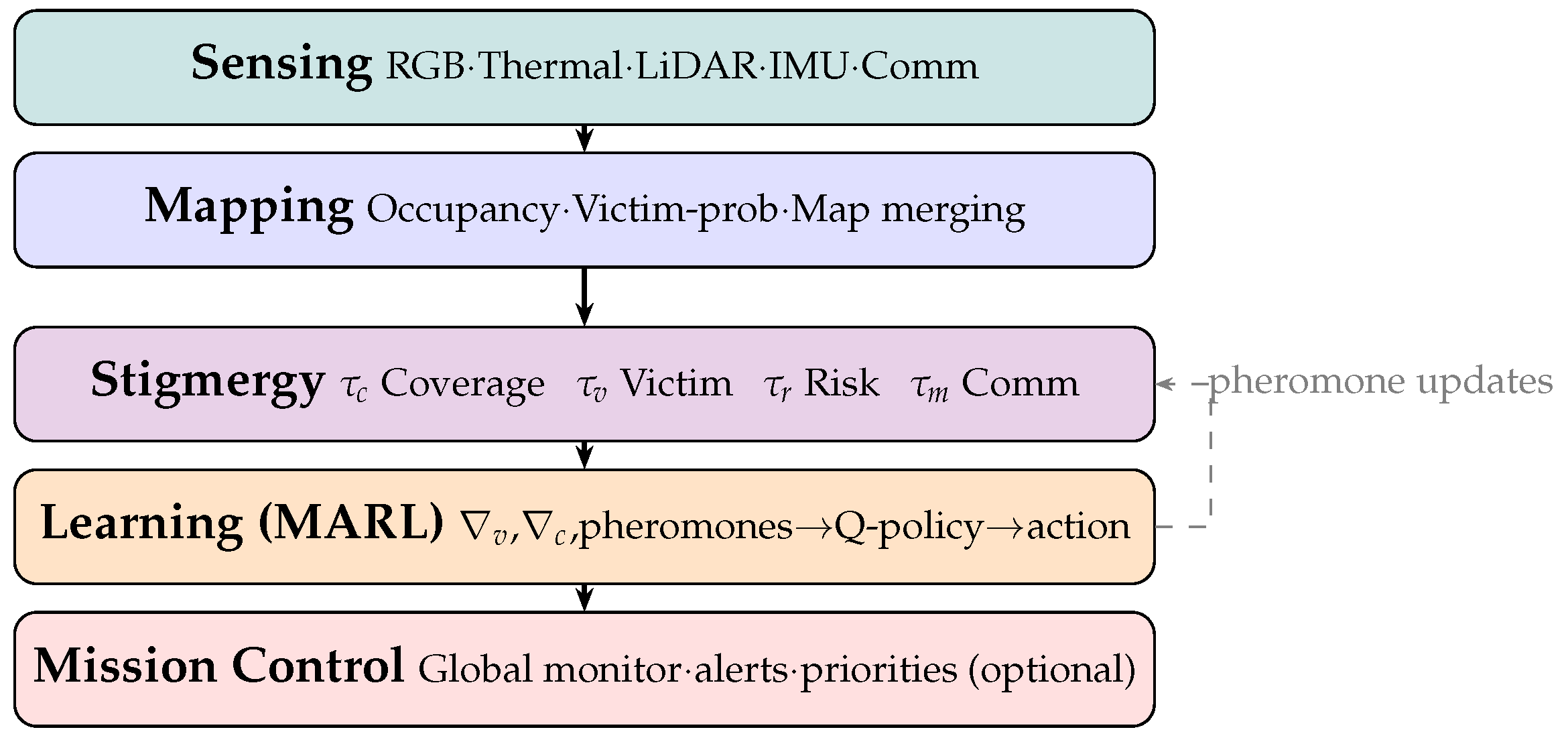
Figure 1.
Five-layer Hybrid stigmergy-RL architecture. The dashed arrow shows pheromone deposits fed back from the learning layer. The learning layer receives directional gradients , computed from the stigmergy layer, not just local scalar values.
Figure 1.
Five-layer Hybrid stigmergy-RL architecture. The dashed arrow shows pheromone deposits fed back from the learning layer. The learning layer receives directional gradients , computed from the stigmergy layer, not just local scalar values.
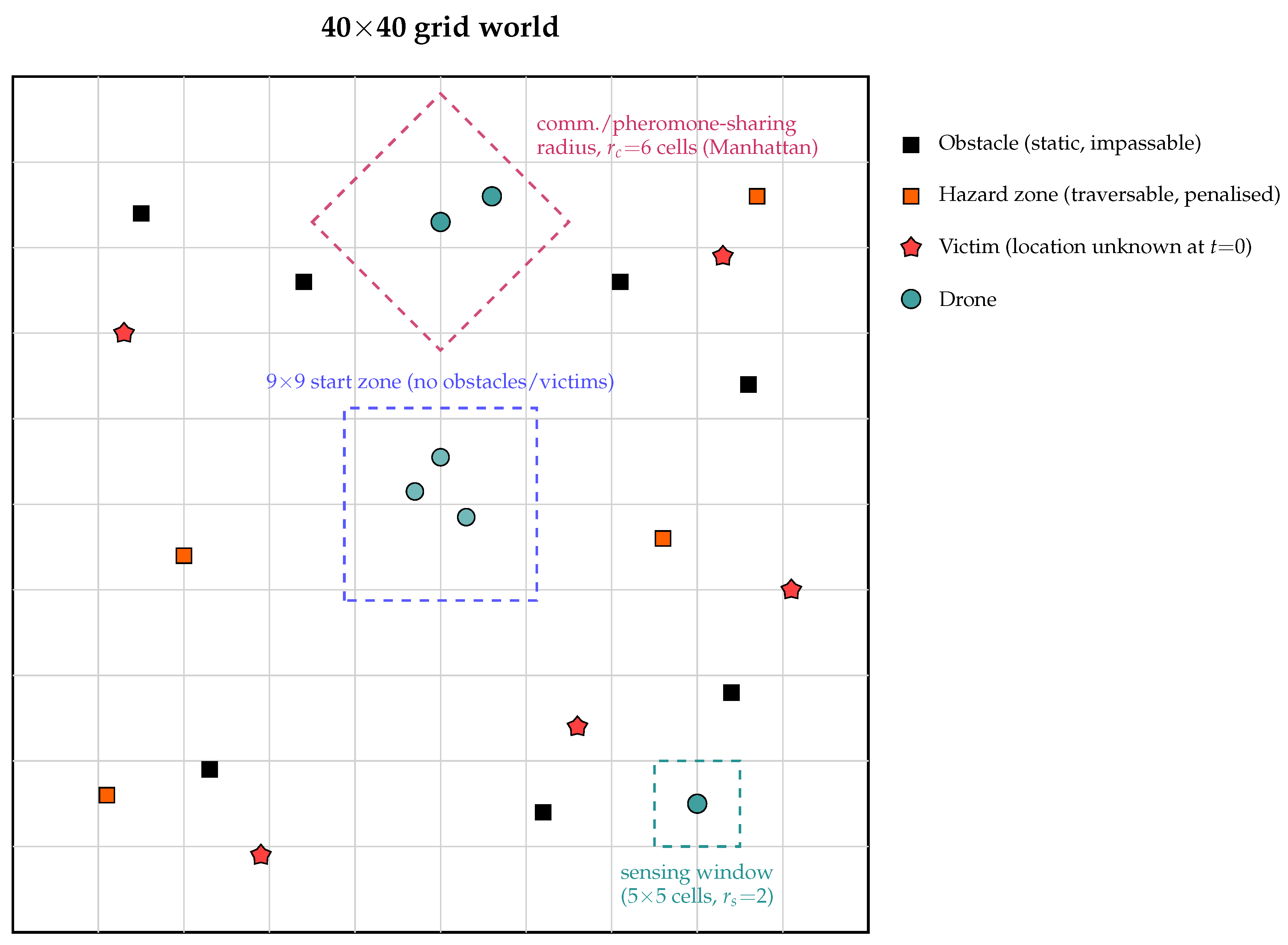
Figure 2.
Schematic of the environment: the central drone-start zone, a single drone’s sensing window (), the communication/pheromone-sharing region ( cells, Manhattan distance), and the three cell types (obstacles, hazard zones, victims).
Figure 2.
Schematic of the environment: the central drone-start zone, a single drone’s sensing window (), the communication/pheromone-sharing region ( cells, Manhattan distance), and the three cell types (obstacles, hazard zones, victims).
Figure 3.
The four independent pheromone layers tracked per grid cell. Each evolves according to Equation (
1) with its own evaporation rate
and diffusion coefficient
; a drone’s observation includes all four values at its current cell (Equation (
2)).
Figure 3.
The four independent pheromone layers tracked per grid cell. Each evolves according to Equation (
1) with its own evaporation rate
and diffusion coefficient
; a drone’s observation includes all four values at its current cell (Equation (
2)).
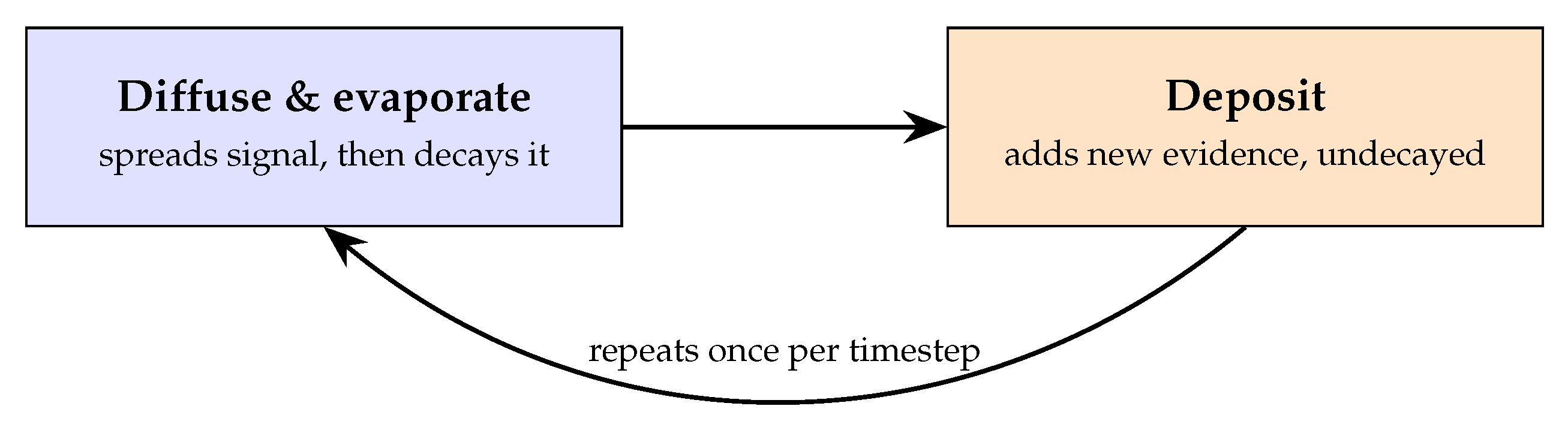
Figure 4.
Per-cell pheromone update cycle (any layer
k). Diffusion and evaporation are applied together each timestep,
, after which new deposits
are added, undecayed, until the following timestep. Together these give
(Equation (
1)).
Figure 4.
Per-cell pheromone update cycle (any layer
k). Diffusion and evaporation are applied together each timestep,
, after which new deposits
are added, undecayed, until the following timestep. Together these give
(Equation (
1)).
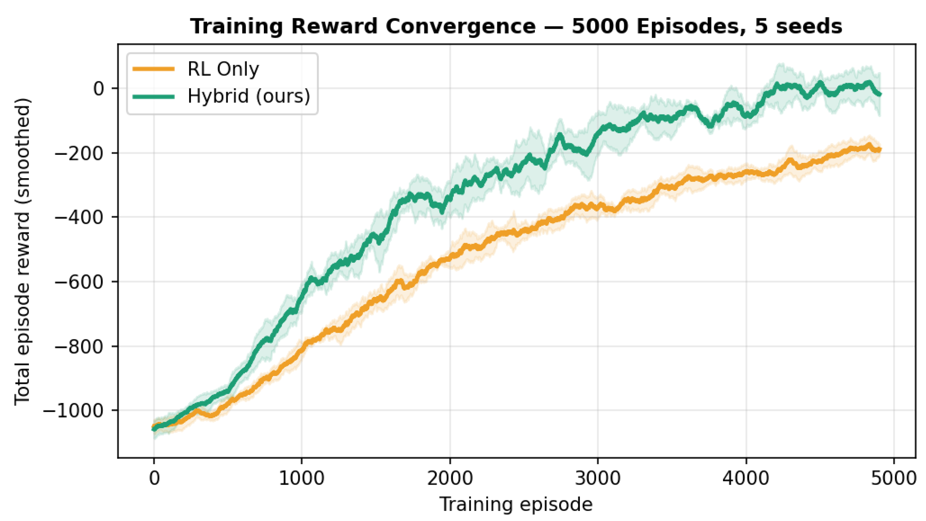
Figure 5.
Training reward convergence across 5000 training episodes for Hybrid and RL-Only models (5 independent random training seeds per model). Curves are smoothed using a 100-episode moving average. Shaded bands represent standard deviation across the five seeds. Experiments were conducted on a grid with 10 drones, 20 victims, 180 obstacles, and 50 hazard zones.
Figure 5.
Training reward convergence across 5000 training episodes for Hybrid and RL-Only models (5 independent random training seeds per model). Curves are smoothed using a 100-episode moving average. Shaded bands represent standard deviation across the five seeds. Experiments were conducted on a grid with 10 drones, 20 victims, 180 obstacles, and 50 hazard zones.
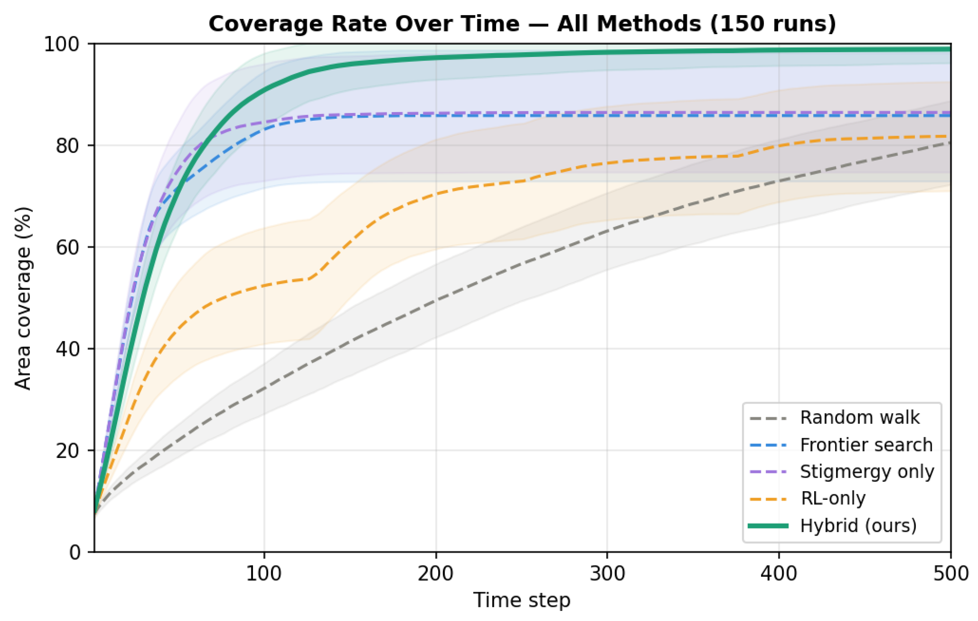
Figure 6.
Mean area coverage percentage over 500 execution timesteps across pooled evaluation runs (30 independent evaluation trials per seed, five training seeds). Shaded regions denote error bands.
Figure 6.
Mean area coverage percentage over 500 execution timesteps across pooled evaluation runs (30 independent evaluation trials per seed, five training seeds). Shaded regions denote error bands.
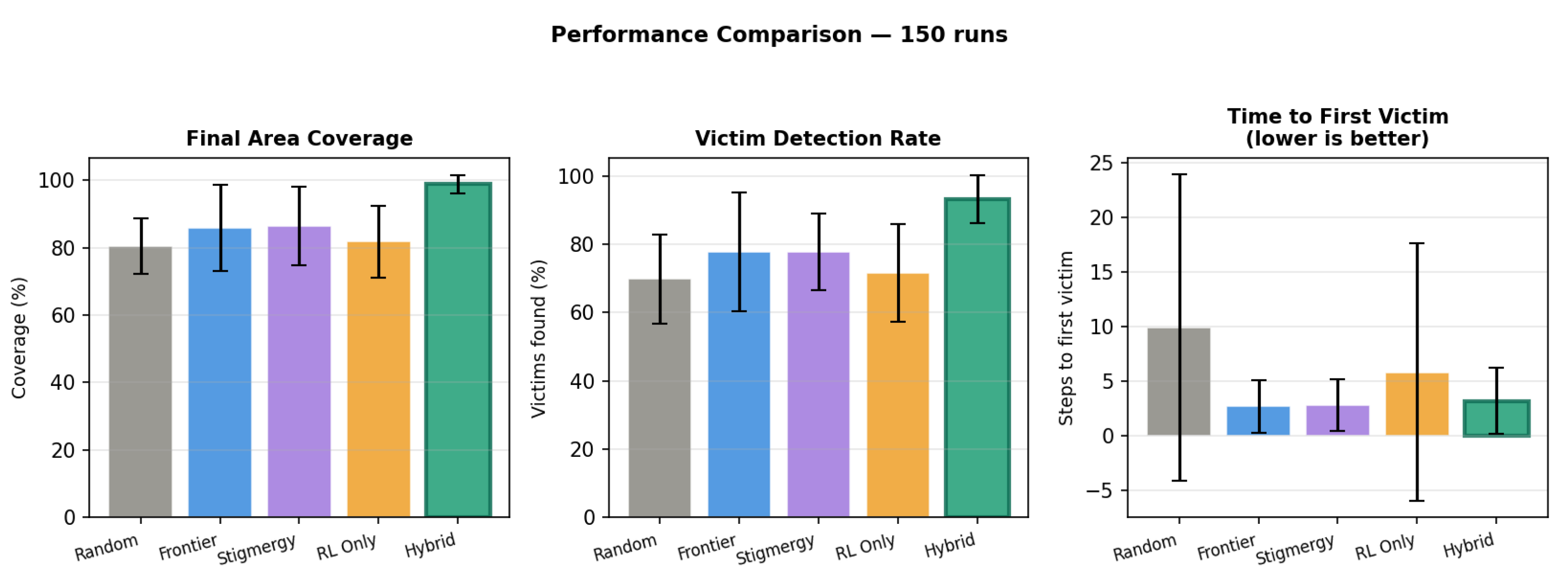
Figure 7.
Comparative performance metrics across pooled evaluation runs (30 independent trials per seed across five training seeds) for five benchmark methods: random walk, Frontier search, Stigmergy-only, RL-only, and the proposed Hybrid model. Lower values indicate better performance for time to first victim (steps), while higher values reflect superior performance in area coverage (%) and victim detection rate (%). Error bars represent standard deviation across all pooled evaluation trials. Testing was conducted on a grid with 10 drones, 20 victims, 180 obstacles, and 50 hazard zones.
Figure 7.
Comparative performance metrics across pooled evaluation runs (30 independent trials per seed across five training seeds) for five benchmark methods: random walk, Frontier search, Stigmergy-only, RL-only, and the proposed Hybrid model. Lower values indicate better performance for time to first victim (steps), while higher values reflect superior performance in area coverage (%) and victim detection rate (%). Error bars represent standard deviation across all pooled evaluation trials. Testing was conducted on a grid with 10 drones, 20 victims, 180 obstacles, and 50 hazard zones.
Figure 8.
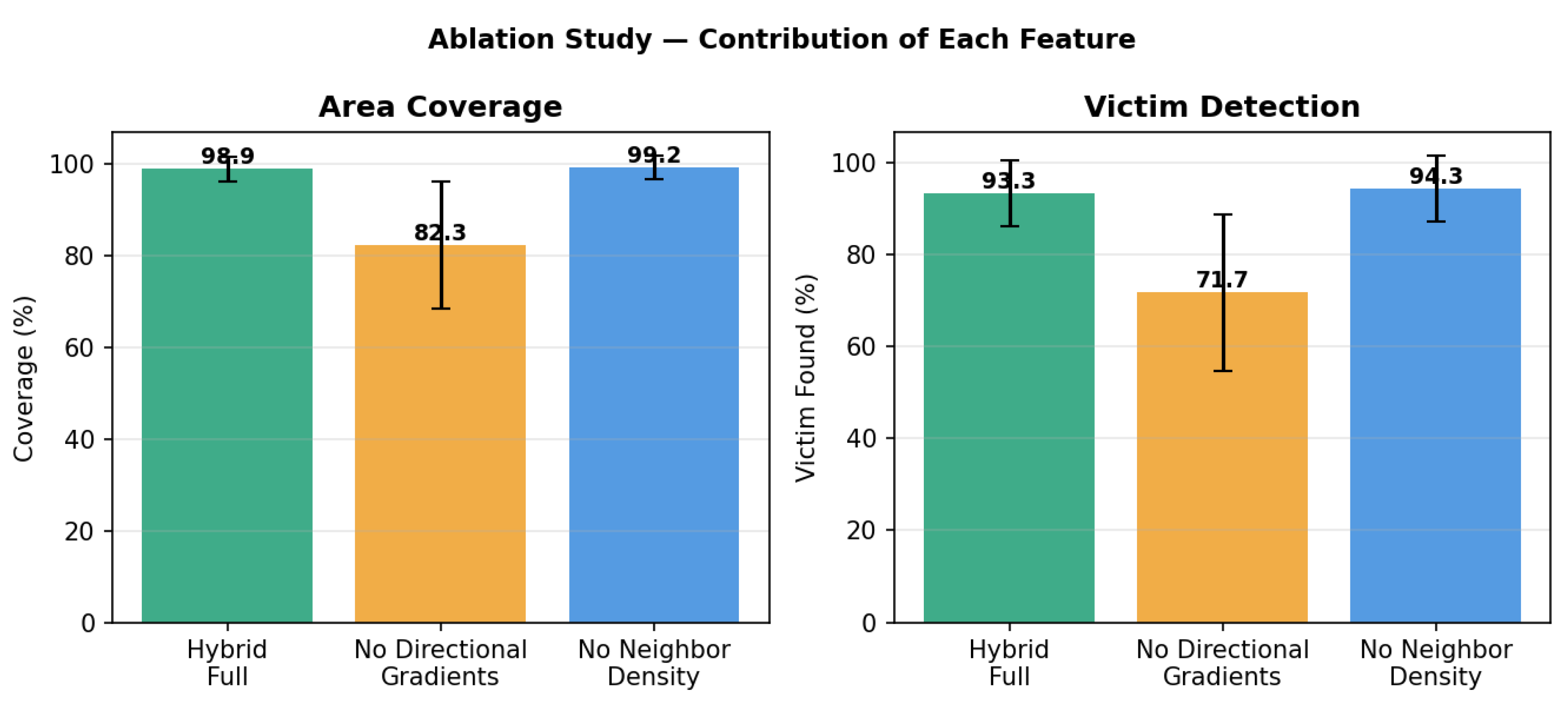
Ablation study showing area coverage (%) and victim detection (%) when removing directional gradients () or neighbor density () ( evaluation runs across five seeds). Error bars reflect standard deviation across all pooled evaluation trials. Directional gradients serve as the primary driver of performance. Evaluated on a grid with 10 drones, 20 victims, 180 obstacles, and 50 hazards.
Figure 8.
Ablation study showing area coverage (%) and victim detection (%) when removing directional gradients () or neighbor density () ( evaluation runs across five seeds). Error bars reflect standard deviation across all pooled evaluation trials. Directional gradients serve as the primary driver of performance. Evaluated on a grid with 10 drones, 20 victims, 180 obstacles, and 50 hazards.
Figure 9.
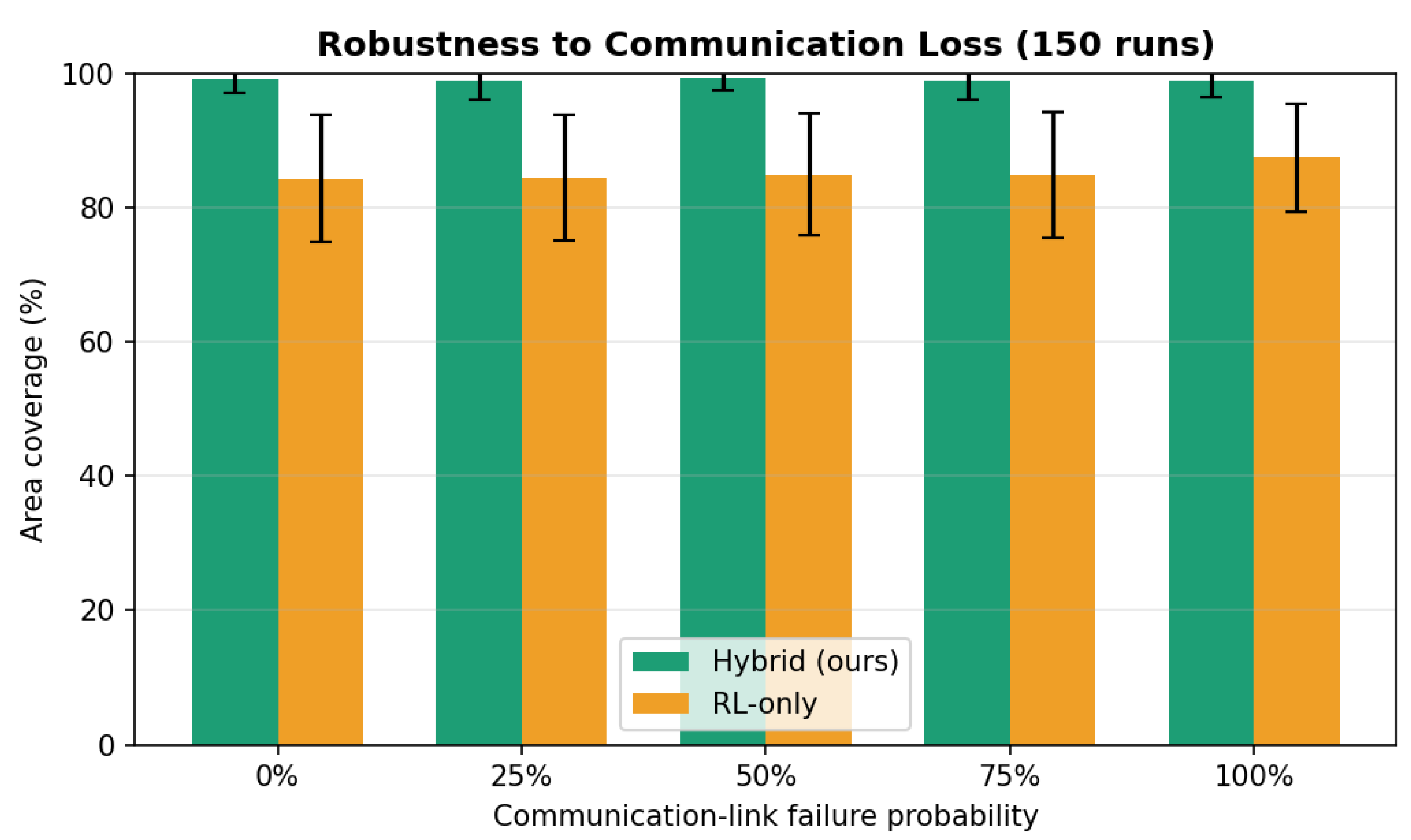
Impact of communication-link failure probability (0–100%) on area coverage for Hybrid vs. RL-only models ( evaluation runs across five seeds). Error bars represent standard deviation. The Hybrid model maintains coverage regardless of dropout rate, preserving a 14–15% advantage over RL-Only. Evaluated on a grid with 10 drones, 20 victims, 180 obstacles, and 50 hazards.
Figure 9.
Impact of communication-link failure probability (0–100%) on area coverage for Hybrid vs. RL-only models ( evaluation runs across five seeds). Error bars represent standard deviation. The Hybrid model maintains coverage regardless of dropout rate, preserving a 14–15% advantage over RL-Only. Evaluated on a grid with 10 drones, 20 victims, 180 obstacles, and 50 hazards.
Table 1.
Multi-UAV SAR modeling Dec-POMDP tuple definitions.
Table 1.
Multi-UAV SAR modeling Dec-POMDP tuple definitions.
| Component | Description |
|---|
| Set of N autonomous drone agents (). |
| Global state space, including grid cell occupancy, static obstacle and hazard coordinates, victim locations, and four-layer virtual pheromone intensities across all cells. |
| Joint action space, where each agent’s discrete action space is . |
| State transition probability function governing movement and environmental virtual pheromone updates like evaporation or diffusion. |
| Individual scalar reward for agent i, , computed from that agent’s own local outcomes (collision, hazard entry, newly-scanned cells, victim detection, energy cost; Equation (3)). |
| is the joint observation space, where agent i receives local observation vector generated by observation function . |
| Discount factor (). |
Table 2.
Comparison between scalar and directional observation representations. Coverage variability is the pooled standard deviation across all 150 evaluation runs; the coverage gain is the absolute increase from RL-only’s 81.8% to Hybrid’s 98.9%.
Table 2.
Comparison between scalar and directional observation representations. Coverage variability is the pooled standard deviation across all 150 evaluation runs; the coverage gain is the absolute increase from RL-only’s 81.8% to Hybrid’s 98.9%.
| Property | Scalar (RL-Only) | Directional (Hybrid) |
|---|
| Observation dimensionality | 9 features | 18 features |
| Coverage variability (std) | 10.8% | 2.7% |
| Mean steps to first victim | 5.8 | 3.2 |
| Coverage gain | — | +17.1% |
Table 3.
Simulation parameters and reward coefficients.
Table 3.
Simulation parameters and reward coefficients.
| Parameter | Description | Value |
|---|
| Grid/Drones/Victims | Environment setup | /10/20 |
| Obstacles/Hazards | Static obstacles/hazard zones | 180/50 |
| Sensing radius | Per-drone view window | 2 cells |
| Comm. radius | Pheromone sharing range | 6 cells |
| Battery budget | Steps per episode | 500 |
| Evaporation rates | 0.05/0.02/0.03/0.04 |
| Diffusion coefficients | 0.08/0.05/0.06/0.07 |
| / | Victim/coverage weight | 5.0/1.0 |
| / | Comm.energy weight | 0.3/0.1 |
| / | Collision/risk penalty | 2.0/1.5 |
| Learning rate | Q-learning step | 0.18 |
| Discount | Future reward | 0.93 |
| schedule | Exp. decay (×0.9996/ep) | 1.0 → 0.135 at ep 5000 |
| Discretization bins | Per pheromone feature | 6 |
| Training episodes/runs | Per agent/eval seeds | 5000/30 |
Table 4.
Policy observation state: Hybrid vs. RL-Only.
Table 4.
Policy observation state: Hybrid vs. RL-Only.
| Feature | Encoding | Hybrid | RL-Only |
|---|
| Local coverage pheromone | 6 bins | ✓ | ✓ |
| Local victim pheromone | 6 bins | ✓ | ✓ |
| Local risk | binary flag | ✓ | ✓ |
| Normalized battery | 4 bins | ✓ | ✓ |
| Obstacle indicators | 4 binary | ✓ | ✓ |
| Victim-gradient direction | N/S/W/E/none | ✓ | — |
| Coverage-gradient direction | N/S/W/E | ✓ | — |
| Neighbor density | 3 bins | ✓ | — |
| Total state dimension | | 18 | 9 |
Table 5.
Statistical significance: Hybrid vs. RL-only (Welch’s t-test, pooled each).
Table 5.
Statistical significance: Hybrid vs. RL-only (Welch’s t-test, pooled each).
| Metric | t | df | p | Cohen’s d |
|---|
| Coverage | 18.88 | 168 | <0.001 | 2.18 |
| Victim detection | 16.49 | 218 | <0.001 | 1.90 |
Table 6.
Ablation study: mean ± Std across five Seeds (30 Runs Each, Pooled ). RMSE vs. Hybrid is the root-mean-square deviation of each variant from the full Hybrid model, computed jointly across the coverage and victim-detection columns.
Table 6.
Ablation study: mean ± Std across five Seeds (30 Runs Each, Pooled ). RMSE vs. Hybrid is the root-mean-square deviation of each variant from the full Hybrid model, computed jointly across the coverage and victim-detection columns.
| Variant | Coverage (%) | Victims (%) | RMSE vs. Hybrid (%) |
|---|
| Hybrid Full (ours) | | | — |
| No directional gradients | | | 19.26 |
| No neighbor density | | | 0.74 |
Table 7.
Evaluation results: mean ± Std across five seeds (30 runs each, pooled ; grid, 10 drones, 20 victims, 500 steps).
Table 7.
Evaluation results: mean ± Std across five seeds (30 runs each, pooled ; grid, 10 drones, 20 victims, 500 steps).
| Method | Coverage (%) | Victims (%) | 1st Victim (Steps) |
|---|
| Random walk | | | |
| Frontier search | | | |
| Stigmergy only | | | |
| RL-only | | | |
| Hybrid (ours) | | | |
Table 8.
Communication-dropout sweep: mean coverage and victims, 150 runs.
Table 8.
Communication-dropout sweep: mean coverage and victims, 150 runs.
| Dropout (%) | Hybrid Cov. (%) | Hybrid Vic. (%) | RL Cov. (%) | RL Vic. (%) |
|---|
| 0 | 99.3 | 93.7 | 84.4 | 73.7 |
| 25 | 99.0 | 93.3 | 84.6 | 73.3 |
| 50 | 99.3 | 93.6 | 85.0 | 73.9 |
| 75 | 98.9 | 93.2 | 84.9 | 74.6 |
| 100 | 99.1 | 91.8 | 87.5 | 76.9 |
Table 9.
Parameter sensitivity analysis across evaporation (), diffusion (D), and learning rate (LR). Metrics represent mean performance across evaluation seeds.
Table 9.
Parameter sensitivity analysis across evaporation (), diffusion (D), and learning rate (LR). Metrics represent mean performance across evaluation seeds.
| Parameter | Scale/Value | Coverage (%) | Victims (%) | 1st Victim (Steps) |
|---|
| Evaporation () | | 97.9 | 90.2 | 2.9 |
| | (base) | 99.8 | 94.0 | 2.9 |
| | | 99.8 | 93.8 | 3.3 |
| | | 99.3 | 94.3 | 3.1 |
| Diffusion (D) | | 98.5 | 93.0 | 2.8 |
| | (base) | 99.8 | 94.0 | 2.9 |
| | | 99.0 | 93.3 | 2.7 |
| | | 99.2 | 93.7 | 2.8 |
| Learning Rate (LR) | (0.09) | 99.8 | 94.0 | 2.9 |
| | (0.18) | 99.8 | 94.0 | 2.9 |
| | (0.27) | 99.8 | 94.0 | 2.9 |
| | (0.36) | 99.8 | 94.0 | 2.9 |