Precision Docking of a Foldable Quadrotor on a Wheel-Legged Robot via CFNTSM with GFA-FEO and FiLM-SAC Deep Reinforcement Learning

Highlights

What are the main findings?

• An air–ground cooperative robotic system is presented, featuring a foldable quadrotor and a small wheel-legged robot that employs electro-permanent magnets for autonomous deployment and retrieval.
• A hierarchical control framework integrating an improved continuous finite-time nonsingular terminal sliding mode controller (CFNTSM), a generalized-fuzzy-approximationbased finite-time extended observer (GFA-FEO), and a feature-wise linear modulation soft actor–critic (FiLM-SAC) deep reinforcement learning policy is developed, enabling sub-centimetre docking precision (<10 mm) and robust payload-adaptive takeoff under a twofold mass increase.

What are the implications of the main findings?

• This framework presents a promising and comprehensively modeled approach toward autonomous air–ground robotic coordination for factory inspection, geographical surveying, and disaster-response missions.
• The proposed control method resolves the severe control-authority degradation during in-flight folding and compensates for gait-induced periodic vibrations.

Abstract

Deploying unmanned aerial vehicles (UAVs) cooperatively with legged robots for disaster response and inspection requires autonomous docking on miniature walking platforms. This study addresses the problem of landing a foldable quadrotor onto the back of a trotting wheel-legged robot ($300\times 180$ mm) and subsequently taking off while carrying it as a payload. Four tightly coupled challenges distinguish this task from conventional mobile-platform landing: (i) an extremely small landing surface, (ii) gait-induced periodic vibrations at $2.5$ Hz, (iii) continuous platform translation at $0.3$–$0.8$ m/s, and (iv) surface docking that requires simultaneous position and attitude matching rather than mere point tracking. The proposed framework comprises four components: (1) a novel single-servo crank-rocker folding mechanism that reduces the folded body footprint by 48.5% and the maximum linear dimension from 590 mm to 309 mm (↓47.6%) compared with the prior dual-servo design; (2) a staged Continuous Fast Nonsingular Terminal Sliding Mode (CFNTSM) controller combined with a Gait-Frequency-Aware Finite-time Extended Observer (GFA-FEO); (3) a Feature-wise Linear Modulation Soft Actor-Critic (FiLM-SAC) residual reinforcement-learning policy conditioned on physical states and mission phase, with an adaptive trust weight $\lambda \left(t\right)$; and (4) a payload-adaptive takeoff strategy with parameter hot-switching to handle the twofold mass increase. Extensive Monte Carlo simulations and ablation studies across three experiment groups demonstrate that the proposed hierarchical framework achieves sub-centimetre (<10 mm) position accuracy and <3° attitude matching on a walking platform. Quantitatively, the full method reduces docking RMSE by 42% relative to the model-based CFNTSM + GFA-FEO controller without residual RL (4.2 vs. 7.2 mm) and reduces post-lock takeoff RMSE by 63% through FEO hot-switching (16.2 vs. 44.2 mm).

1. Introduction

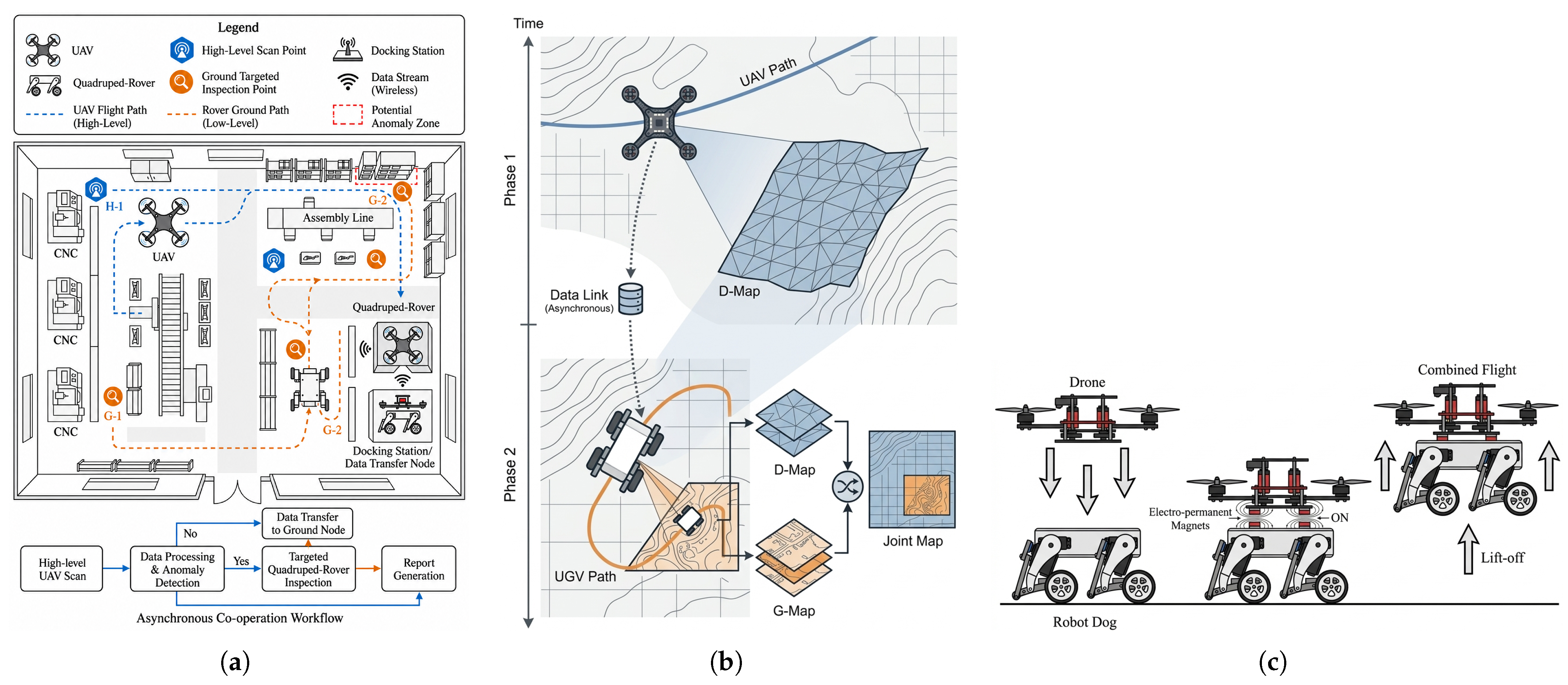
Disaster response, post-earthquake reconnaissance, hazardous industrial inspection, and large-scale geographic surveys all require the terrain-traversing capability of legged robots and the three-dimensional mobility of unmanned aerial vehicles (UAVs). Recent air–ground robotic systems exploit this complementarity for precision farming, collaborative perception, navigation, and cooperative localization [1,2,3,4]. However, most such systems treat aerial and ground robots as independent cooperative agents rather than integrated bodies that must physically dock, lock, and relaunch. An attractive operational concept involves a quadrotor that carries a miniature wheel-legged robot over obstacles, deploys it with precision, and subsequently re-docks and retrieves it (Figure 1). During inactive phases, the UAV remains stowed on the robot’s back with minimal power consumption.

Our system pairs a foldable quadrotor with a compact wheel-legged robot (back surface $300\times 180$ mm). Docking is achieved via electro-permanent magnets (EPMs): the robot’s back carries a steel plate, while the UAV’s underside mounts four corner EPMs. A foldable airframe is essential because (i) the deployed propeller span (∼420 mm) far exceeds the 180 mm back width, and protruding blades would collide with swinging legs; (ii) the folded UAV forms a compact backpack with minimal drag; and (iii) a reduced footprint lowers collision risk in confined spaces.

This scenario introduces four tightly coupled challenges that distinguish it from conventional UAV landing settings:

1.

Tiny landing surface with gait-induced vibration. The landing surface is extremely compact (EPM tolerance ±30 mm), while the trot gait at $2.5$ Hz produces ±5 mm vertical and ±2.0°/±1.5° roll/pitch oscillations; the robot walks at 0.3–0.8 m/s throughout docking.

2.

Surface docking, not point tracking. The UAV must match a rigid, tilting surface—not merely track a point—with tolerances $\parallel \mathrm{\Delta }{\mathbf{p}}_{xy}\parallel <10$ mm, $\left|\mathrm{\Delta }\varphi \right|,\left|\mathrm{\Delta }\theta \right|<3^{°}$, and $|\dot{z}|<0.1$ m/s (Section 2.5).

3.

Fold-induced control-authority loss. Folding substantially reduces motor moment arms and introduces transient zero-crossing singularities, degrading attitude authority precisely when millimetre-level alignment is required (Section 2.2.2).

4.

Payload-adaptive takeoff with mass doubling. At EPM lock the coupled mass approximately doubles, the centre of mass shifts, and the inertia tensor changes abruptly while the arms must unfold to restore authority.

Prior work has addressed several parts of this problem. Air–ground robot teams have been studied for collaborative perception, occlusion-aware navigation, GNSS-challenged localization, formation control, and task allocation [1,2,3,4,5,6,7,8]. UAV landing on moving platforms has also been investigated using visual servoing, visual–inertial guidance, shipboard landing, and MPC-based methods [9,10,11,12]. These studies provide the cooperative and target-tracking background, but they usually assume loose air–ground coupling or comparatively large rigid landing areas rather than a small gait-excited robot back that must become mechanically locked to the UAV.

Aerial manipulation, grasping, and perching show how contact can extend the role of UAVs beyond free flight [13,14,15,16]. In parallel, morphing and foldable UAVs demonstrate that mechanical reconfiguration can improve access, agility, or mission versatility while introducing configuration-dependent dynamics [17,18,19,20,21,22,23,24,25]. However, these works mainly address branches, walls, gaps, perching, or free-flight morphing; they do not link fold-angle-dependent moment arms to surface docking tolerances and post-lock coupled-body dynamics.

Learning-enhanced UAV control and simulation have recently improved agile flight, residual compensation, and robust tracking under disturbances [26,27,28,29,30,31,32,33,34,35,36,37,38]. Yet existing learning and observer designs rarely condition residual authority simultaneously on fold angle, gait state, and mission phase, and they do not address the observer reset caused by a sudden mass/inertia jump after EPM locking. The missing link is therefore a unified formulation for a foldable quadrotor that must dock on a small vibrating walking-robot’s back and then take off with the robot as payload.

These gaps motivate four objectives: (G1) precision surface docking with fold-induced moment-arm degradation; (G2) exploit periodic gait structure jointly with fold-angle-dependent authority; (G3) physically conditioned, phase-aware residual RL with an adaptive trust weight; (G4) payload-adaptive takeoff after EPM locking under an abrupt mass/inertia change.

The main contributions are:

1.

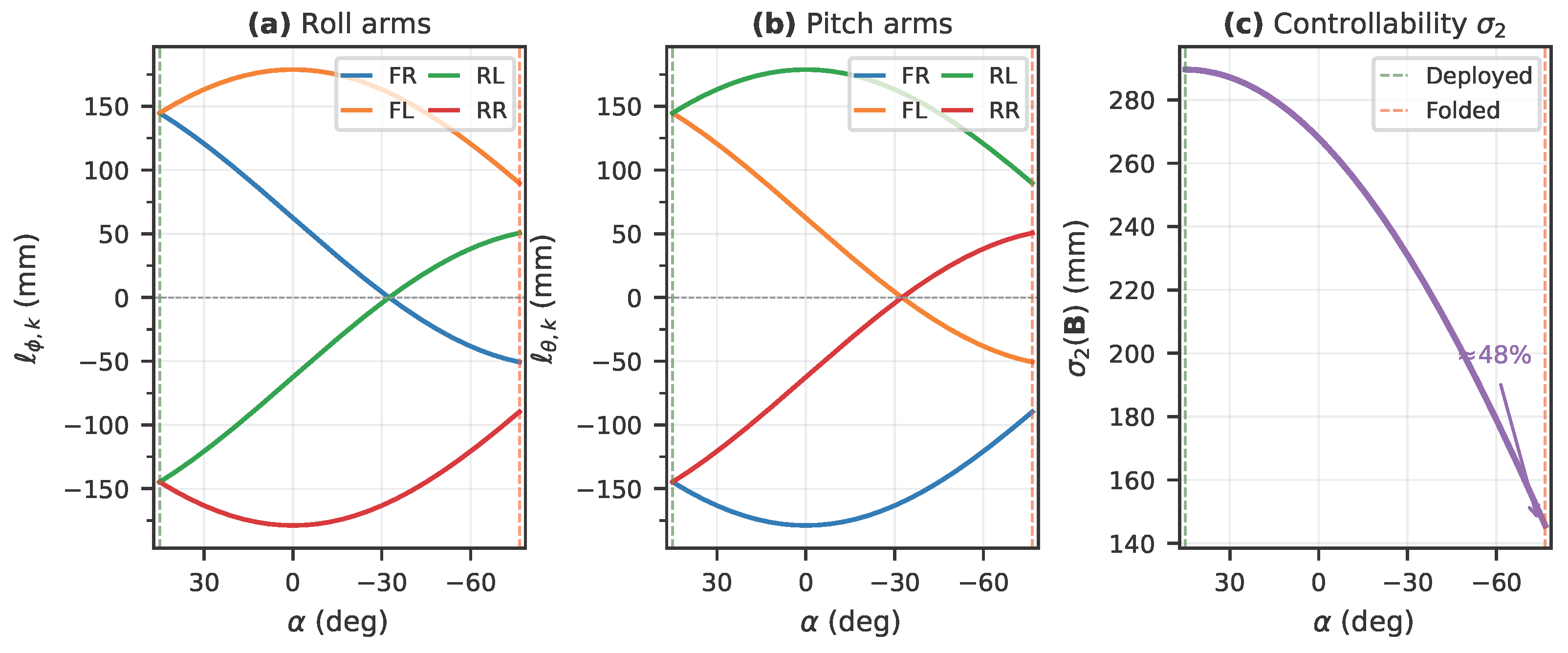
Fold-induced coupling analysis and surface-docking formulation (G1). We derive the closed-form dependence of $\mathbf{B}\left(\alpha \right)$ and $\mathbf{J}\left(\alpha \right)$ on fold angle $\alpha$, revealing how a ${121.5}^{°}$ shuriken fold degrades ${\sigma }_2\left(\mathbf{B}\right)$ by $48\%$ and transiently drives motor moment arms through zero. To the best of our knowledge, this is the first fold-angle-dependent surface-docking model for a foldable quadrotor landing on a walking platform.

2.

Staged CFNTSM with GFA-FEO (G2). A gait-frequency-aware finite-time extended observer fuses velocity differencing, ESO, and a periodic internal model tuned to $f_g$; the CFNTSM operates with FSM-scheduled gains and activates enhanced-gain mode during terminal descent.

3.

FiLM-SAC residual RL with adaptive $\lambda \left(t\right)$ (G3). A residual policy conditioned via FiLM on fold state, gait parameters, and mission phase is modulated by an adaptive trust weight $\lambda \left(t\right)$ based on tracking error, observer residual, and FSM transition signals, extending fixed-weight residual formulations.

4.

Payload-adaptive takeoff with FEO hot-switching (G4). Upon EPM locking, an FEO hot-switch protocol updates the plant model and resets observer states; the FiLM-SAC residual bridges the re-convergence blind window for stable takeoff from the stowed state.

The rest of this paper is organised as follows. Section 2 derives the dynamic model. Section 3 presents the three-layer controller and FSM. Section 4 details PSO optimisation. Section 5 reports simulation results. Section 6 discusses findings and limitations. Section 7 concludes.

2. System Description and Dynamic Modelling

This section presents the hardware configuration of the air–ground cooperative system, derives the folding kinematics and fold-dependent moment arms of the single-servo mechanism, and establishes the dynamic models for the foldable quadrotor, the walking-legged robot, and the coupled body formed upon docking.

The model equations are derived by combining geometric mechanism closure with rigid-body dynamics. The folding linkage is first reduced to a planar four-bar loop-closure problem, yielding Freudenstein’s relation and the fold angle $\alpha$ as the mechanism configuration variable. The motor locations are then obtained from the arm-pivot geometry, and the control moment arms are derived from the cross product $\mathbf{\tau }=\mathbf{r}\times \mathbf{F}$. The quadrotor translation and rotation equations follow the Newton–Euler formulation in the body frame, with $\mathbf{B}\left(\alpha \right)$ and $\mathbf{J}\left(\alpha \right)$ updated from the fold geometry. The walking platform is represented by a kinematic gait-excitation model whose dominant frequencies are set by stride length and walking speed, while the post-docking body is obtained by mass aggregation and the parallel-axis theorem. Ground effect is included as an empirical near-surface thrust correction during docking and takeoff.

2.1. System Overview and Coordinate Frames

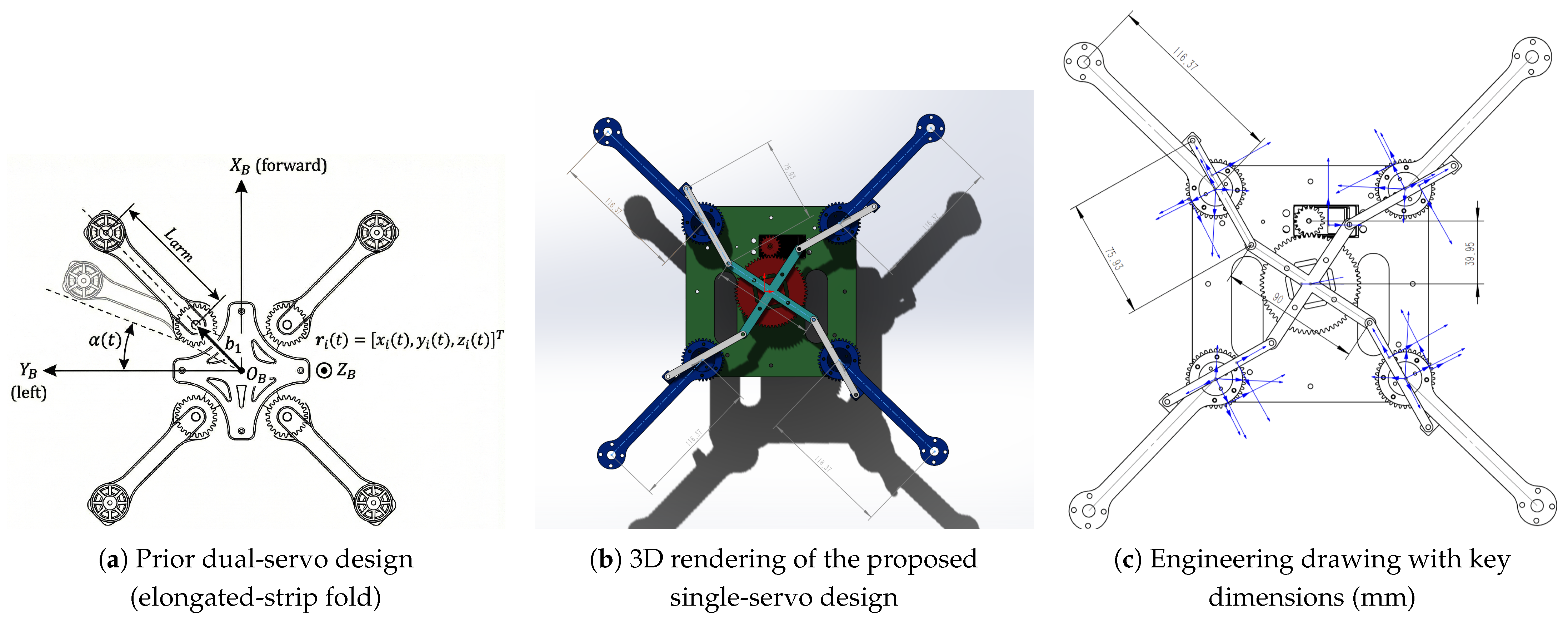
The system comprises two agents: a foldable quadrotor ($m_u=2.50$ kg) and a wheel-legged robot ($m_d=2.50$ kg, back surface $300\times 180$ mm). The folding mechanism and hardware configuration are detailed in Section 2.2; Figure 2 shows the prior dual-servo design alongside the proposed crank-rocker design for direct comparison.

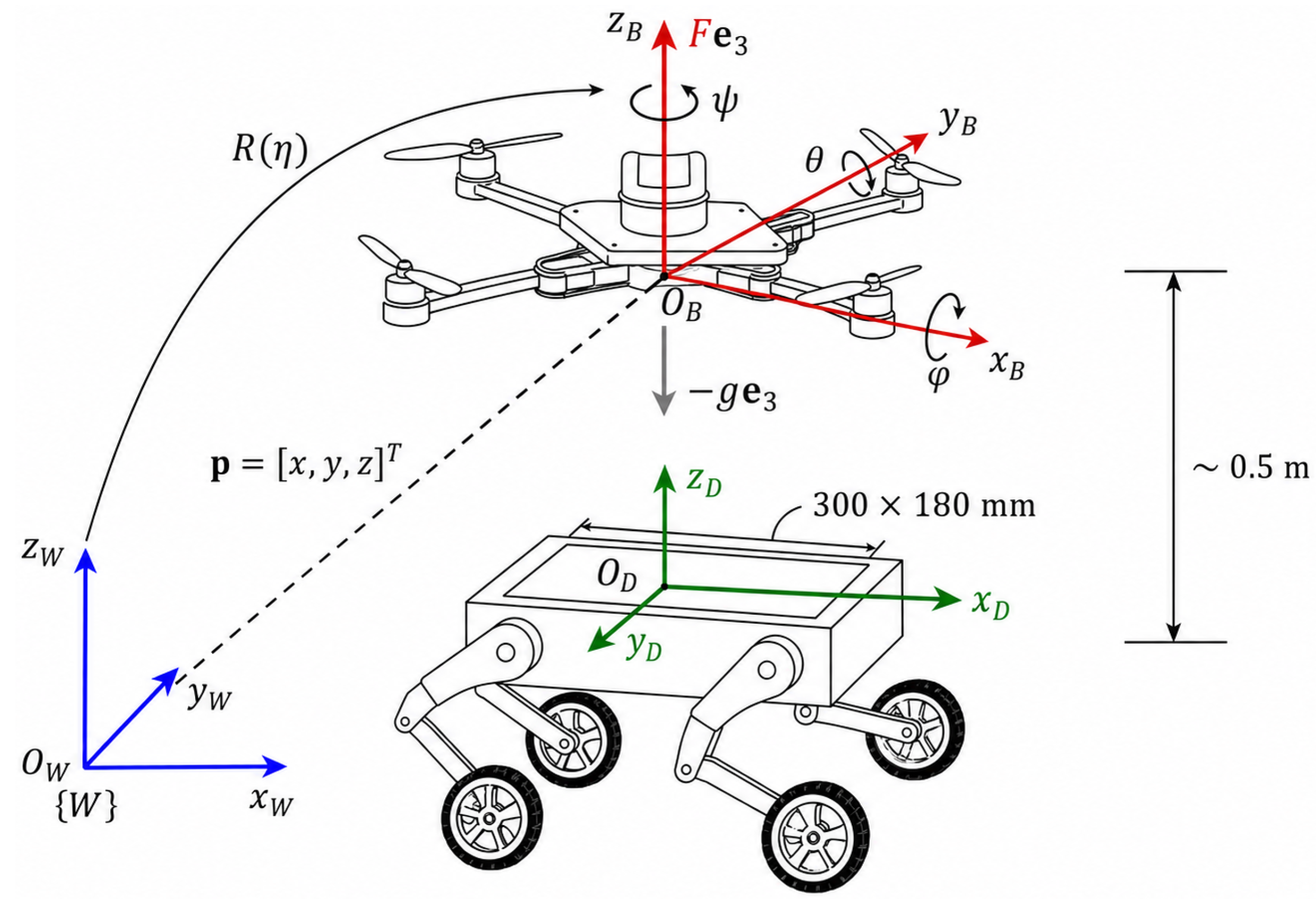
Three right-handed coordinate frames are used throughout (Figure 3). The world frame $\left\{W\right\}$ is Earth-fixed with the z-axis pointing upward (ENU convention). The body frame $\left\{B\right\}$ has its origin at the UAV centre of mass, $z_B$ along the thrust axis, $x_B$ pointing toward arm 1 (front-right in the deployed X-configuration); Euler angles $\mathit{\eta }={[\varphi ,\theta ,\psi ]}^T$ (roll, pitch, yaw) describe the rotation from $\left\{W\right\}$ to $\left\{B\right\}$ via the ZYX convention. The dog frame $\left\{D\right\}$ is centred on the robot’s back surface, with $x_D$ along the walking direction and $z_D$ normal to the back surface.

2.2. Single-Servo Crank-Rocker Folding Mechanism

The folding mechanism supplies the configuration variable used by the allocation and inertia models. The single-servo architecture defines the geometric constraints, the four-bar loop closure maps servo motion to fold angle, and the resulting motor positions determine the moment arms available to the controller.

2.2.1. Mechanism Design

The folding mechanism adopts the single-servo four-bar crank-rocker architecture demonstrated by Tuna et al. [22], who validated a 0.6 s fold/deploy cycle in the FOLLY quadcopter. However, FOLLY’s flight experiments were conducted exclusively in the fully deployed configuration; the effects of in-flight morphing on dynamics and control authority were not investigated. The present work fills this gap by deriving the fold-angle-dependent allocation matrix $\mathbf{B}\left(\alpha \right)$ and embedding $\alpha$ into both the dynamic model and the control design.

The airframe uses a $150\times 150$ mm square base plate with four arms ($L_a=116$ mm) attached at corner pivots. A central servo drives a 18/62-tooth gear pair ($n_g=3.44:1$ reduction), a cross-shaped crank ($r_c=45$ mm), and four connecting rods ($l_r=75.93$ mm) that synchronise all arms. Compared to the prior dual-servo design (Figure 2a), the single-servo mechanism reduces the folded body footprint from 88,500 mm² to 45,546 mm² (−48.5%), the maximum linear dimension from 590 mm to 309 mm (−47.6%), and eliminates front/rear servo synchronisation. The $n_g=3.44:1$ gear reduction is selected primarily to preserve torque margin for the $2.50$ kg airframe and the four-arm linkage, rather than to pursue faster morphing than FOLLY. In the commanded fold/deploy profile used by the simulations, the servo traverses ${205}^{°}$ over $T_{\mathrm{fold}}=0.6$ s, so the mechanism retains the same nominal deployment-time benchmark while trading excess speed for higher output torque at the crank. The controller uses the measured/commanded fold angle $\alpha \left(t\right)$ rather than assuming instantaneous deployment; if hardware load tests require a slower profile, the same model remains valid after updating $T_{\mathrm{fold}}$.

2.2.2. Kinematics, Fold Geometry, and Moment Arms

Each arm’s motion is governed by a planar four-bar linkage (ground link $G=88.4$ mm, crank $r_c=45$ mm, coupler $l_r=75.93$ mm, output link $d_e=32.16$ mm). The loop-closure yields Freudenstein’s relation:

$$K_{1}cos\varphi -K_{2}cos{\theta }_c+K_3=cos({\theta }_c-\varphi ),$$

(1)

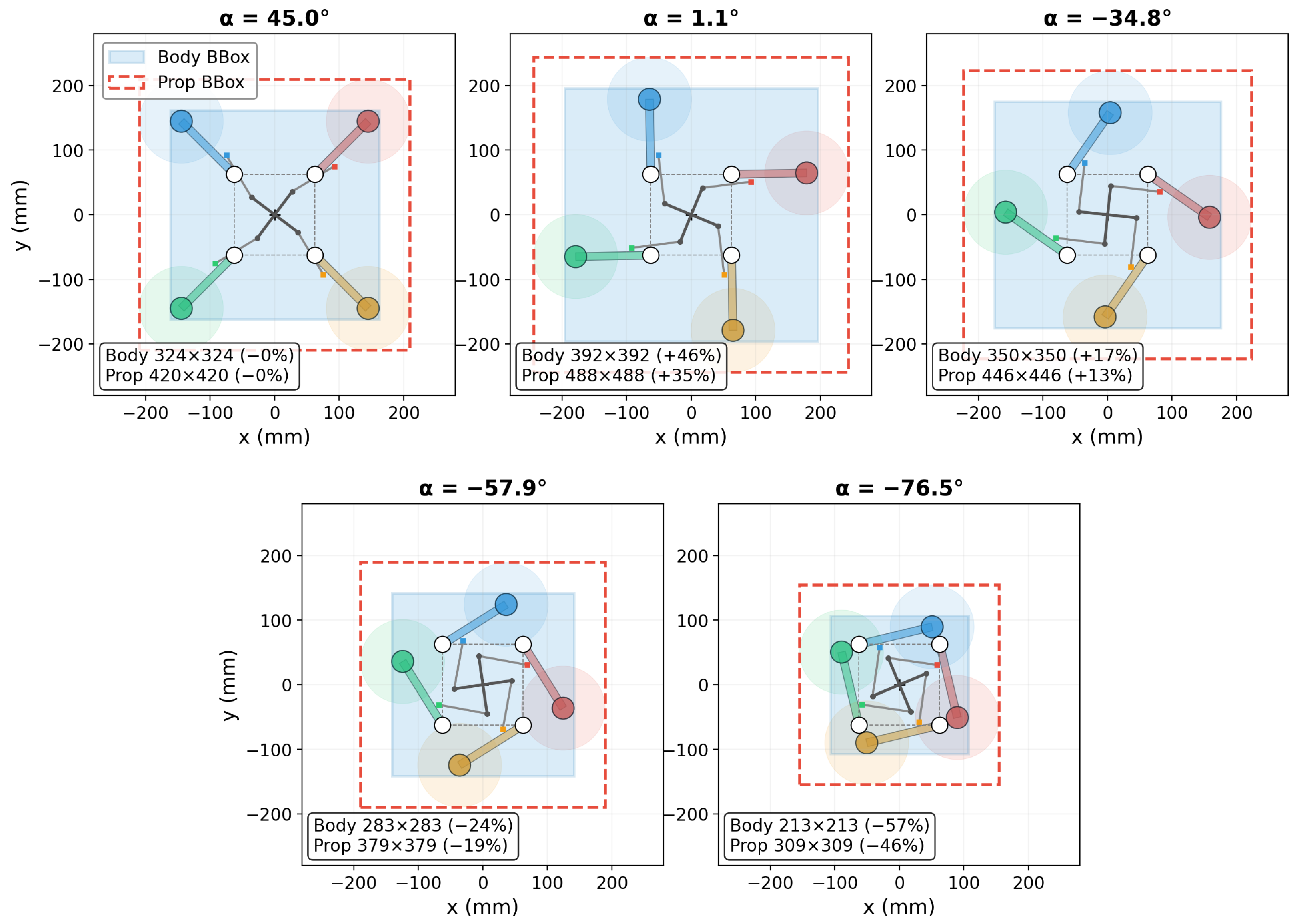
with $K_1=G/r_c$, $K_2=G/d_e$, $K_3=(d_e^2-l_r^2+r_c^2+G^2)/\left(2r_c{d}_e\right)$. The mechanism satisfies the Grashof condition ($d_e+G<r_c+l_r$ by 0.3 mm). Because this margin is small, the prototype does not rely on the Grashof inequality alone for mechanical robustness. The practical design uses a finite mechanical end-stop, clearance at the pin joints, and a slew-limited servo command to keep the linkage away from a high-speed toggle crossing. Thermal expansion over the expected indoor/outdoor operating range is much smaller than the link lengths and is absorbed by the joint clearances, while any rise in fold-servo current or a mismatch between commanded and measured $\alpha$ can be used as a jamming indicator in the hardware implementation. A crank rotation of ${59.55}^{°}$ (servo travel ${205}^{°}$, 76% utilisation) drives each arm through $\mathrm{\Delta }\alpha ={121.5}^{°}$: from the deployed X-configuration ($\alpha ={45}^{°}$) through a transient +-pattern ($\alpha \approx 0^{°}$) to the fully folded shuriken at ${\alpha }_{\mathrm{fold}}=-{76.5}^{°}$ (Figure 4). The propeller-tip bounding box contracts from $420\times 420$ mm to $309\times 309$ mm (−45.6% area); the folding-body envelope reaches $213\times 213$ mm when folding propellers are considered. The mechanical end-stop is set by motor-housing–pivot-shaft contact at $\alpha =-{76.6}^{°}$.

The motor positions and moment arms are computed directly from the arm-pivot geometry. Arm k pivots at ${\mathbf{P}}_k$ on the $125\times 125$ mm pivot square and carries its motor at radius $L_a$. The motor position is:

$${\mathbf{p}}_{m,k}\left({\alpha }_k\right)={\mathbf{P}}_k+L_a\left[\begin{array}{c}cos{\alpha }_k\\ sin{\alpha }_k\end{array}\right],$$

(2)

where $a_f=125/2=62.5$ mm. The roll and pitch moment arms follow from $\mathbf{\tau }=\mathbf{r}\times \mathbf{F}$:

$$l_{\varphi ,k}\left({\alpha }_k\right)=a_{f,y,k}+L_{a}sin{\alpha }_k,l_{\theta ,k}\left({\alpha }_k\right)=-(a_{f,x,k}+L_{a}cos{\alpha }_k).$$

(3)

At deployment ($\alpha ={45}^{°}$) all motors have equal moment arms $|l_{\varphi ,k}|=144.8$ mm; at full fold the average drops to ∼70 mm ($-52\%$), and individual motors transiently pass through zero moment arms at intermediate angles ($\alpha \approx -{33}^{°}$), creating control-authority singularities that necessitate the gain-scheduled controller of Section 3.5 (Figure 5).

2.3. Foldable Quadrotor Dynamics

The following standard assumptions are adopted for the foldable-quadrotor model:

• A1. The airframe (central plate, arms, and motors) is rigid; structural deformation during folding is negligible.
• A2. Roll and pitch angles are bounded in $(-\pi /2,\pi /2)$, and the yaw angle is bounded in $(-\pi ,\pi )$.
• A3. External disturbances (wind, ground effect, and gait coupling) and their time derivatives are bounded: $\parallel {\mathbf{d}}_{\mathrm{ext}}\parallel \le \overline{d}$, $\parallel {\dot{\mathbf{d}}}_{\mathrm{ext}}\parallel \le {\overline{d}}_1$, $\parallel {\mathbf{\tau }}_{\mathrm{ext}}\parallel \le \overline{\tau }$, $\parallel {\dot{\mathbf{\tau }}}_{\mathrm{ext}}\parallel \le {\overline{\tau }}_1$.

2.3.1. Thrust, Attitude, and Translational Dynamics

Each rotor k ($k=1,\dots ,4$) spins at angular speed ${\mathrm{\Omega }}_k$ and produces a thrust force and a reactive drag torque along $z_B$:

$$f_k=k_f{\mathrm{\Omega }}_k^2,{\tau }_{d,k}=k_{\tau }{\mathrm{\Omega }}_k^2,$$

(4)

where $k_f$ and $k_{\tau }$ are the thrust and torque coefficients, respectively. The total thrust is $F={\sum }_{k=1}^4{f}_k$. The torque-to-thrust ratio is $c_{\tau }=k_{\tau }/k_f$. Rotors 1 and 3 spin clockwise (CW), rotors 2 and 4 counter-clockwise (CCW); their spin-direction sign is ${\sigma }_k\in \{-1,+1,-1,+1\}$, so that the net yaw torque vanishes in hover.

For the attitude kinematics, let $\mathit{\eta }={[\varphi ,\theta ,\psi ]}^T$ denote the ZYX Euler angles (roll, pitch, yaw) from $\left\{W\right\}$ to $\left\{B\right\}$. The corresponding rotation matrix $\mathbf{R}\in SO\left(3\right)$ that maps body-frame vectors to the world frame is:

$$\mathbf{R}\left(\mathit{\eta }\right)=\left[\begin{array}{ccc}{c}_{\theta }{c}_{\psi }& s_{\varphi }{s}_{\theta }{c}_{\psi }-c_{\varphi }{s}_{\psi }& c_{\varphi }{s}_{\theta }{c}_{\psi }+s_{\varphi }{s}_{\psi }\\ c_{\theta }{s}_{\psi }& s_{\varphi }{s}_{\theta }{s}_{\psi }+c_{\varphi }{c}_{\psi }& c_{\varphi }{s}_{\theta }{s}_{\psi }-s_{\varphi }{c}_{\psi }\\ -s_{\theta }& s_{\varphi }{c}_{\theta }& c_{\varphi }{c}_{\theta }\end{array}\right],$$

(5)

where $c_{(·)}=cos(·)$ and $s_{(·)}=sin(·)$.

The relation between the Euler–angle rates $\dot{\mathit{\eta }}$ and the body angular velocity $\mathit{\omega }={[p,q,r]}^T$ is:

$$\dot{\mathit{\eta }}={\mathbf{W}}^{-1}\left(\mathit{\eta }\right)\mathit{\omega },$$

(6)

with

$${\mathbf{W}}^{-1}=\left[\begin{array}{ccc}1& s_{\varphi }{t}_{\theta }& c_{\varphi }{t}_{\theta }\\ 0& c_{\varphi }& -s_{\varphi }\\ 0& s_{\varphi }/c_{\theta }& c_{\varphi }/c_{\theta }\end{array}\right],$$

(7)

where $t_{\theta }=tan\theta$. Note that ${\mathbf{W}}^{-1}$ is singular at $\theta =\pm \pi /2$, which is excluded by Assumption A2.

For translation, let $\mathbf{p}={[x,y,z]}^T$ denote the UAV centre-of-mass position in $\left\{W\right\}$. The translational dynamics are:

$$m\ddot{\mathbf{p}}=\mathbf{R}\left(\mathit{\eta }\right)F{\mathbf{e}}_3-mg{\mathbf{e}}_3+{\mathbf{d}}_{\mathrm{ext}},$$

(8)

where m is the (possibly time-varying) system mass, F the total thrust from (4), $\mathbf{R}$ the rotation matrix (5), and ${\mathbf{d}}_{\mathrm{ext}}$ the external disturbance satisfying Assumption A3.

Since the arms rotate in the horizontal plane, all propellers remain vertical. Thrust efficiency remains constant (${\eta }_T=1.0$) for all fold angles $\alpha$, indicating that folding does not compromise vertical thrust generation.

2.3.2. Rotational Dynamics with Variable Moment Arms

Defining the angular-momentum vector $\mathbf{G}\left(\alpha \right)=\mathbf{J}\left(\alpha \right)\mathit{\omega }$, the rotational dynamics follow from Euler’s equation in the body frame:

$$\dot{\mathbf{G}}\left(\alpha \right)=\mathbf{J}\left(\alpha \right)\dot{\mathit{\omega }}+\dot{\mathbf{J}}\left(\alpha \right)\mathit{\omega }=-\mathit{\omega }\times \mathbf{J}\left(\alpha \right)\mathit{\omega }+{\mathbf{\tau }}_{\mathrm{ctrl}}+{\mathbf{\tau }}_G+{\mathbf{\tau }}_D+{\mathbf{\tau }}_{\mathrm{ext}},$$

(9)

where the terms on the right-hand side are, respectively, the gyroscopic cross-coupling, the control torque from differential thrust, the rotor gyroscopic torque, the aerodynamic drag torque, and the external disturbance torque.

Remark 1. 

When the fold angle α varies in flight, the inertia tensor changes with time and $\dot{\mathbf{J}}\ne \mathbf{0}$. In the proposed docking manoeuvre, the folding motion is scheduled during the early descent phase and completed before the terminal capture window, so that $\dot{\alpha }=0$ during the critical landing segment and $\dot{\mathbf{J}}=\mathbf{0}$. When folding does occur in flight (e.g., during cruise), the ratio $\parallel \dot{\mathbf{J}}\mathit{\omega }\parallel /\parallel \mathbf{J}\dot{\mathit{\omega }}\parallel$ is small because the fold transition (≈0.6 s) is much slower than the rotational dynamics; this term is therefore absorbed into ${\mathbf{\tau }}_{\mathrm{ext}}$ and handled by the observer (Section 3).

Modelling each arm-plus-motor assembly as a point mass $m_a$ at position ${\mathbf{p}}_{m,k}$ from (2), the inertia tensor about the body-frame origin is:

$$\mathbf{J}\left(\alpha \right)={\mathbf{J}}_0+{\displaystyle \sum _{k=1}^4}{m}_a\left[{\parallel {\mathbf{p}}_{m,k}\left(\alpha \right)\parallel }^2{\mathbf{I}}_3-{\mathbf{p}}_{m,k}\left(\alpha \right){\mathbf{p}}_{m,k}^T\left(\alpha \right)\right],$$

(10)

where ${\mathbf{J}}_0$ is the central-body inertia (batteries, electronics, frame plate) and $m_a$ is the lumped mass of one arm assembly (arm tube, motor, propeller, ESC). Owing to the four-fold shuriken symmetry (${\alpha }_k={\alpha }_1+(k-1)·{90}^{°}$), the products of inertia vanish for all $\alpha$ and $\mathbf{J}\left(\alpha \right)$ remains diagonal:

$$\mathbf{J}\left(\alpha \right)=\mathrm{diag}\left(J_{xx}\left(\alpha \right),J_{yy}\left(\alpha \right),J_{zz}\left(\alpha \right)\right),$$

(11)

with $J_{xx}=J_{yy}$ (roll and pitch inertias are equal) due to the ${90}^{°}$ rotational symmetry. Since all arm masses lie in the $z_B=0$ plane, $J_{zz}\left(\alpha \right)=J_{xx}\left(\alpha \right)+J_{yy}\left(\alpha \right)$ by the perpendicular-axis theorem and likewise varies with $\alpha$.

The control torque ${\mathbf{\tau }}_{\mathrm{ctrl}}$ is produced by differential thrust via the allocation matrix:

$${\mathbf{\tau }}_{\mathrm{ctrl}}\left(\alpha \right)=\mathbf{B}\left(\alpha \right)\mathbf{f},\mathbf{f}={[f_1,f_2,f_3,f_4]}^T,$$

(12)

where the allocation matrix $\mathbf{B}\left(\alpha \right)$ encodes the $\alpha$-dependent moment arms from (3):

$$\mathbf{B}\left(\alpha \right)=\left[\begin{array}{cccc}{y}_{m,1}& y_{m,2}& y_{m,3}& y_{m,4}\\ -x_{m,1}& -x_{m,2}& -x_{m,3}& -x_{m,4}\\ {\sigma }_1{c}_{\tau }& {\sigma }_2{c}_{\tau }& {\sigma }_3{c}_{\tau }& {\sigma }_4{c}_{\tau }\end{array}\right],$$

(13)

with $c_{\tau }=k_{\tau }/k_f$ the torque-to-thrust ratio and ${\sigma }_k\in \{-1,+1,-1,+1\}$ the propeller spin-direction sign (rotors 1, 3 CW; rotors 2, 4 CCW).

The reactive gyroscopic torque due to spinning rotors is:

$${\mathbf{\tau }}_G={\displaystyle \sum _{k=1}^4}{J}_r(\mathit{\omega }\times {\mathbf{e}}_3){\sigma }_k{\mathrm{\Omega }}_k,$$

(14)

where $J_r$ is the rotor moment of inertia about its spin axis. This term is small in near-hover but becomes non-negligible during aggressive attitude manoeuvres or rapid motor speed changes.

The body drag force from rotor downwash and the associated drag torque are modelled as:

$${\mathbf{\tau }}_D=-k_d\mathrm{diag}(1,1,1)\mathit{\omega },$$

(15)

where $k_d>0$ is the lumped aerodynamic drag coefficient.

As $\alpha$ changes, $\mathbf{B}\left(\alpha \right)$ varies continuously, introducing roll–pitch cross-coupling that compounds the moment-arm degradation analysed in Section 2.2.2.

2.3.3. Ground Effect and Model Parameters

During the terminal descent ($h<0.3$ m above the robot’s back) and at takeoff, the thrust is amplified by ground effect. We adopt the Cheeseman–Bennett model:

$$K_{\mathrm{GE}}\left(h\right)={\displaystyle \frac{1}{1-{(R_p/4h)}^2}},$$

(16)

where h is the distance from the propeller disc to the nearest ground surface (or robot back surface). As $h\to R_p/4$, $K_{\mathrm{GE}}\to \infty$, producing strong thrust perturbations in the final approach. During near-surface flight, the effective thrust in (8) is replaced by $F_{\mathrm{eff}}=K_{\mathrm{GE}}\left(h\right)F$.

The model parameters in the preceding equations are fixed before controller design so that the control and optimisation sections can be interpreted against a single physical platform.

Table 1. Quadrotor dynamic-model parameters.

Parameter	Symbol	Value
Total mass	m	2.50 kg
Arm assembly mass (each)	$m_a$	0.18 kg
Arm length (pivot to motor)	$L_a$	116 mm
Propeller radius	$R_p$	65 mm
Thrust coefficient	$k_f$	$1.5\times {10}^{-5}$ N$·$s2
Torque coefficient	$k_{\tau }$	$2.4\times {10}^{-7}$ N$·$m$·$s2
Torque-to-thrust ratio	$c_{\tau }$	0.016 m
Rotor inertia	$J_r$	$3.8\times {10}^{-5}$ kg$·$m2
Aerodynamic drag coeff.	$k_d$	$2.5\times {10}^{-3}$ N$·$m$·$s
Roll/pitch inertia (deployed)	$J_{xx}^{\mathrm{dep}}$	$1.2\times {10}^{-2}$ kg$·$m2
Roll/pitch inertia (folded)	$J_{xx}^{\mathrm{fold}}$	$5.8\times {10}^{-3}$ kg$·$m2
Yaw inertia (deployed)	$J_{zz}^{\mathrm{dep}}$	$2.1\times {10}^{-2}$ kg$·$m2
Yaw inertia (folded)	$J_{zz}^{\mathrm{fold}}$	$1.0\times {10}^{-2}$ kg$·$m2

summarises the key physical and aerodynamic values used in the dynamic model, including the deployed and folded inertia values that drive the fold-aware gain scheduling.

2.4. Walking Robot Platform Model

The walking robot contributes a moving, periodically tilted landing surface. For docking control, the dominant effects are the stride-driven heave, roll, and pitch components at the robot’s back. The gait frequency is therefore estimated from robot geometry and walking speed, then mapped into the 6-DoF pose of the landing surface.

Gait-Induced Surface Pose Model

This model converts the walking speed of the ground robot into the time-varying pose of the landing surface. The first step estimates the dominant gait frequency, and the second maps this frequency into the heave, roll, and pitch components tracked by the UAV controller.

The gait frequency serves as the fundamental excitation frequency for the GFA-FEO internal model. Estimating it from robot walking speed and leg-defined stride length enables changes in robot velocity to be mapped directly into the observer harmonics.

The trot stride length is set by the leg geometry and dynamic similarity [39]:

$$l_{\mathrm{stride}}\approx l_{\mathrm{leg}}=L_{\mathrm{thigh}}+L_{\mathrm{shank}},$$

(17)

yielding:

$$f_g={\displaystyle \frac{v}{l_{\mathrm{stride}}}}={\displaystyle \frac{v}{l_{\mathrm{leg}}}}.$$

(18)

For the target robot ($L_{\mathrm{thigh}}=0.10$ m, $L_{\mathrm{shank}}=0.10$ m, nominal $v=0.5$ m/s): $f_g=0.5/0.20=2.5$ Hz. The operating range $v\in [0.3,0.8]$ m/s maps to $f_g\in [1.5,4.0]$ Hz.

The UAV controller tracks the landing surface rather than the ground robot centre. Therefore, the gait excitation is added to the nominal dog pose at the back-surface frame, producing the time-varying position and roll–pitch attitude that define the docking reference.

The landing surface centre position and attitude are:

$$\begin{array}{cc}\hfill {\mathbf{p}}_{\mathrm{land}}\left(t\right)& ={\mathbf{p}}_{\mathrm{dog}}\left(t\right)+{\mathbf{R}}_{\mathrm{dog}}{[0,0,h_{\mathrm{back}}]}^T,\hfill \end{array}$$

(19)

$$\begin{array}{cc}\hfill {\mathit{\eta }}_{\mathrm{land}}\left(t\right)& ={\mathit{\eta }}_{\mathrm{dog}}\left(t\right)+\mathrm{\Delta }{\mathit{\eta }}_{\mathrm{gait}}\left(t\right),\hfill \end{array}$$

(20)

where $\mathrm{\Delta }{\mathit{\eta }}_{\mathrm{gait}}$ is the gait-induced oscillation:

$$\mathrm{\Delta }{\mathit{\eta }}_{\mathrm{gait}}\left(t\right)=\left[\begin{array}{c}{A}_{\varphi }sin(2\pi (f_g/2)t+{\phi }_{\varphi })\\ A_{\theta }sin(2\pi f_{g}t+{\phi }_{\theta })\\ 0\end{array}\right],\mathrm{\Delta }{z}_{\mathrm{gait}}\left(t\right)=A_{z}sin(2\pi ·2f_g·t+{\phi }_z).$$

(21)

Typical amplitudes: $A_{\varphi }\approx {1.5}^{°}$ (roll, at $f_g/2$), $A_{\theta }\approx {2.0}^{°}$ (pitch, at $f_g$), $A_z\approx 5$ mm (heave, at $2f_g$).

2.5. Docking Interface and Coupled-Body Transition

The docking interface links the pre-lock capture condition to the post-lock dynamic model. Before the EPM is energised, the UAV must enter the capture window in position, attitude, and vertical contact speed. After magnetic locking, the vehicle and ground robot are treated as a rigid coupled body for payload-adaptive takeoff.

The EPM array can only capture the steel plate if position, attitude, and contact velocity are simultaneously within tolerance. These physical limits define the docking event used by the FSM and by the simulation success metrics.

A docking attempt is deemed successful if and only if, at the instant of EPM activation, all of the following hold simultaneously:

$$\begin{array}{|c|}\hline \begin{array}{cc}\hfill \parallel {\mathbf{p}}_{\mathrm{UAV},xy}-{\mathbf{p}}_{\mathrm{land},xy}\parallel & <10\mathrm{mm},\hfill \\ \hfill |{\varphi }_{\mathrm{UAV}}-{\varphi }_{\mathrm{land}}|& <3^{°},\hfill \\ \hfill |{\theta }_{\mathrm{UAV}}-{\theta }_{\mathrm{land}}|& <3^{°},\hfill \\ \hfill |{\dot{z}}_{\mathrm{contact}}|& <0.1\mathrm{m}/\mathrm{s},\hfill \\ \hfill |\dot{\varphi }|,|\dot{\theta }|& \approx 0\mathrm{rad}/\mathrm{s}.\hfill \end{array}\\ \hline\end{array}$$

(22)

After EPM locking, the UAV no longer behaves as the original 2.50 kg airframe. The takeoff model uses a rigid coupled body whose mass doubles, whose centre of mass shifts toward the ground robot, and whose inertia tensor is updated by the parallel-axis theorem.

Upon EPM locking, the UAV and robot form a rigid coupled body:

$$\begin{array}{cc}\hfill m_c& =m_u+m_d=2.50+2.50=5.00\mathrm{kg}\left(\mathrm{twofold}\mathrm{mass}\mathrm{increase}\right),\hfill \end{array}$$

(23)

$$\begin{array}{cc}\hfill {\mathbf{p}}_{\mathrm{CoM}}& ={\displaystyle \frac{m_u{\mathbf{p}}_u+m_d{\mathbf{p}}_d}{m_c}},\hfill \end{array}$$

(24)

$$\begin{array}{cc}\hfill {\mathbf{J}}_c& ={\mathbf{J}}_u\left(\alpha \right)+{\mathbf{J}}_d+m_d\left[{\parallel \mathbf{d}\parallel }^2{\mathbf{I}}_3-\mathbf{d}{\mathbf{d}}^T\right],\hfill \end{array}$$

(25)

where $\mathbf{d}={\mathbf{p}}_d-{\mathbf{p}}_{\mathrm{CoM}}$ and the parallel-axis theorem is applied. The translational and rotational dynamics (8) and (9) remain valid with the substitutions $(m,\mathbf{J})\leftarrow (m_c,{\mathbf{J}}_c)$.

2.6. Experimental Prototype Platform

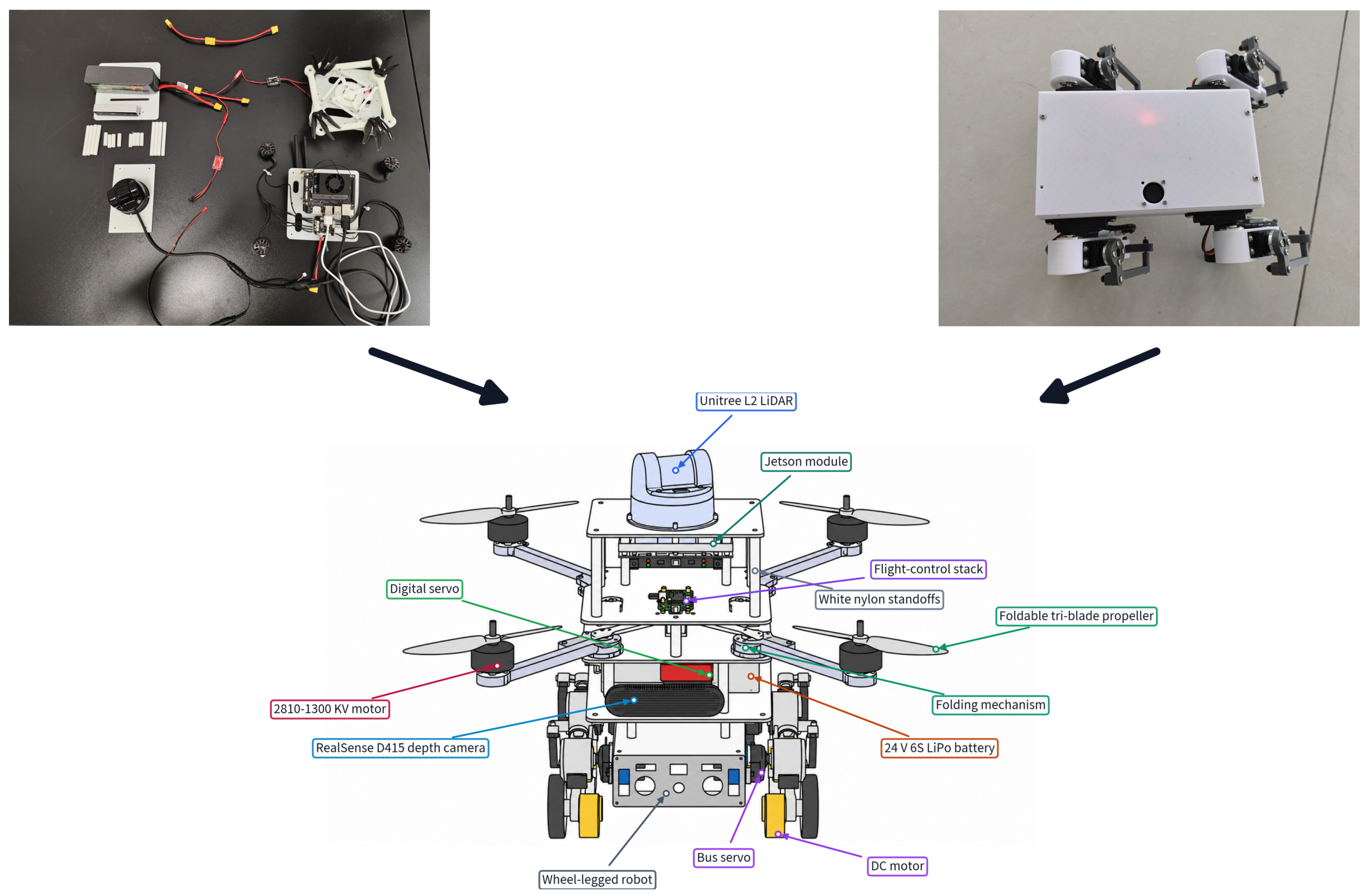
To support the proposed system concept beyond simulation, a full-scale hardware prototype has been designed and assembled. The platform comprises two agents and the resulting hardware layout, including the sensing, compute, folding, propulsion, and ground-robot communication modules, is summarised in Figure 6.

2.6.1. Foldable Quadrotor (Aerial Segment)

The airframe is a custom-designed multi-layer foldable frame that implements the crank-rocker mechanism of Section 2.2 with four 2810-1300 KV BLDC motors (Epower, Shanghai, China), a 70 A 4-in-1 ESC (MicroAir Technology, Shenzhen, Guangdong, China), and a 20 kg digital servo (Xinhui Power Technology, Shenzhen, Guangdong, China) driving the fold linkage via a custom-built 5 V UBEC (Nanjing Tech University, Nanjing, China). The avionics stack is organised in four tiers: Level 1 houses a 6S 5300 mAh 75C LiPo battery (AHTECH, Xuzhou, Jiangsu, China) and an Intel RealSense D415 depth camera (Intel Corporation, Santa Clara, CA, USA). Level 2 carries the foldable frame with gear–crank–connecting-rod mechanism, BLDC motors, servo, and 5 V UBEC. Level 3 hosts an NVIDIA Jetson Orin Nano (NVIDIA Corporation, Santa Clara, CA, USA) running the proposed CFNTSM + GFA-FEO + FiLM-SAC stack and a MicroAir743v2 flight controller (MicroAir Technology, Shenzhen, Guangdong, China; PX4 firmware v1.16.0), communicating via USB-C; the Jetson also drives the fold servo over a PWM signal line. Level 4 mounts a Unitree L2 4D LiDAR (Unitree Robotics, Hangzhou, China) powered by a dedicated custom-built 12 V UBEC (Nanjing Tech University, Nanjing, China). A separate custom-built UPS module (12 V; Nanjing Tech University, Nanjing, China) provides independent power to the Jetson. The docking interface uses the custom-built EPM array (Nanjing Tech University, Nanjing, China) mating with a custom-fabricated Q235 galvanised-steel plate (Nanjing Tech University, Nanjing, China) on the robot’s back.

2.6.2. Wheel-Legged Robot Dog (Ground Segment)

The ground platform is a custom-built quadruped robot (Nanjing Tech University, Nanjing, China) with hybrid wheel–leg locomotion. A custom-built STM32-based main board (Nanjing Tech University, Nanjing, China) coordinates all actuators and communicates with a custom-built handheld controller (Nanjing Tech University, Nanjing, China) via a custom-built ESP32 radio module (Nanjing Tech University, Nanjing, China). Each leg is driven by a crank-rocker linkage with two bus servos (Hiwonder Technology, Shenzhen, Guangdong, China) ($4\times 2$), while four DC TT geared motors (Hongyu Electronic Technology, Shenzhen, Guangdong, China) ($4\times 1$) on each wheel enable continuous wheeled travel. An onboard IMU streams gait orientation data to the UAV through the ESP32 wireless link, providing the GFA-FEO with the prior gait-frequency estimate ${\hat{f}}_g$. Power is supplied by a custom-built rechargeable 3 × 18,650 battery module (Nanjing Tech University, Nanjing, China). This bi-directional data link ensures that the aerial controller receives real-time gait phase information without relying on an external motion-capture system.

2.6.3. Relative-Pose Sensing Pipeline

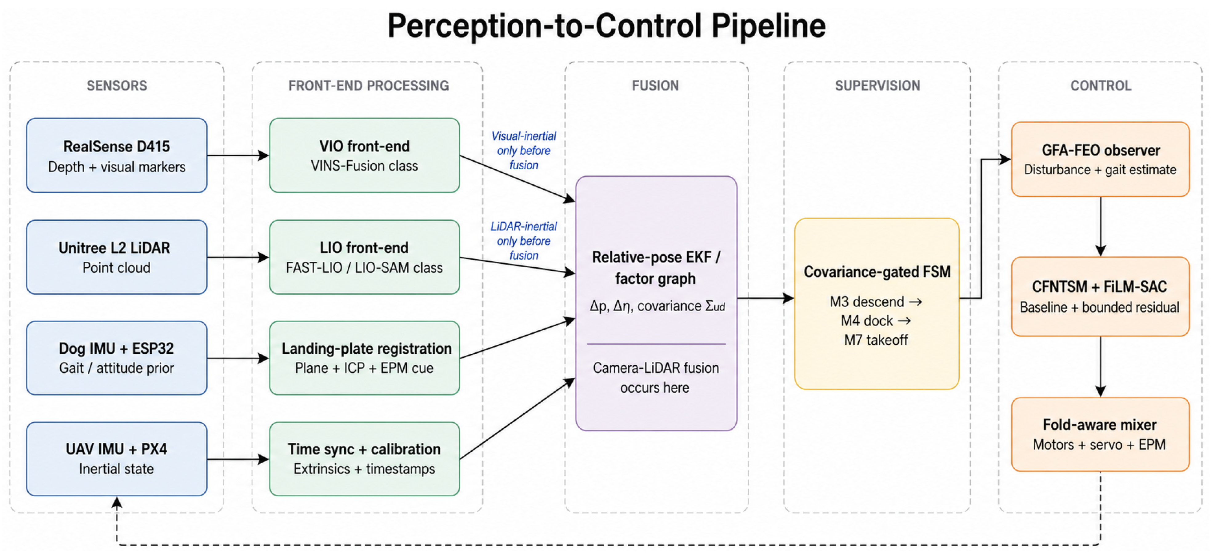
The controller requires the relative pose $\mathrm{\Delta }{\mathbf{x}}_{ud}=(\mathrm{\Delta }\mathbf{p},\mathrm{\Delta }\mathit{\eta })$ between the UAV and the robot back during the final docking phases. In the simulation experiments, this quantity is provided to the controller as a noisy relative-pose measurement; the noise level is consistent with the sensor-noise floor used in the performance-ceiling analysis (${\sigma }_p=0.5$ mm per position channel, Section 3.7). For the assembled hardware prototype, the intended onboard pipeline separates the visual and LiDAR front ends and fuses them at the state-estimation layer. VINS-Fusion is a suitable representative visual–inertial front end for the D415/IMU stream, whereas the FAST-LIO family and LIO-SAM are suitable LiDAR–inertial front ends for the Unitree L2/IMU stream [40,41,42]. They are therefore not claimed to be single camera–LiDAR fusion algorithms; instead, their odometry and registration residuals are transformed into a common robot-deck/UAV frame using offline extrinsic calibration and time synchronisation. At long and medium range, the Unitree L2 point cloud provides a coarse robot/deck pose through plane extraction and ICP-based registration to the known landing-plate geometry. At short range, the RealSense D415 refines the estimate using depth-assisted fiducial/edge detection around the EPM plate; this vision update is used for the final $M_4$ dock entry test. The dog IMU and ESP32 link provide a roll/pitch and gait-phase prior, and an EKF (or equivalent factor-graph estimator) fuses the VIO increments, LiDAR–inertial odometry, LiDAR registration residuals, depth-camera pose residuals, UAV inertial data, and gait prior into the relative pose and covariance used by the FSM.

The $M_4$ transition is therefore gated by both the estimated pose and its covariance: if the lateral uncertainty exceeds the millimetre-level docking margin or the attitude uncertainty approaches the $3^{°}$ capture limit, the FSM remains in align or descend instead of energising the EPM. The present study reports simulation-level validation of the controller under the above measurement-noise model: implementing and experimentally validating the full onboard fusion stack is part of the planned hardware tests. The conversion from sensing outputs to docking/takeoff control inputs is detailed in Figure 7.

3. Hierarchical Control Design

This section presents the three-layer hierarchical controller for precision docking and payload-adaptive takeoff. The overall architecture adopts a position–attitude dual-loop cascade: the outer (position) loop generates desired attitude commands, and the inner (attitude) loop produces torque commands that are mapped to individual motor thrusts via a fold-aware mixer.

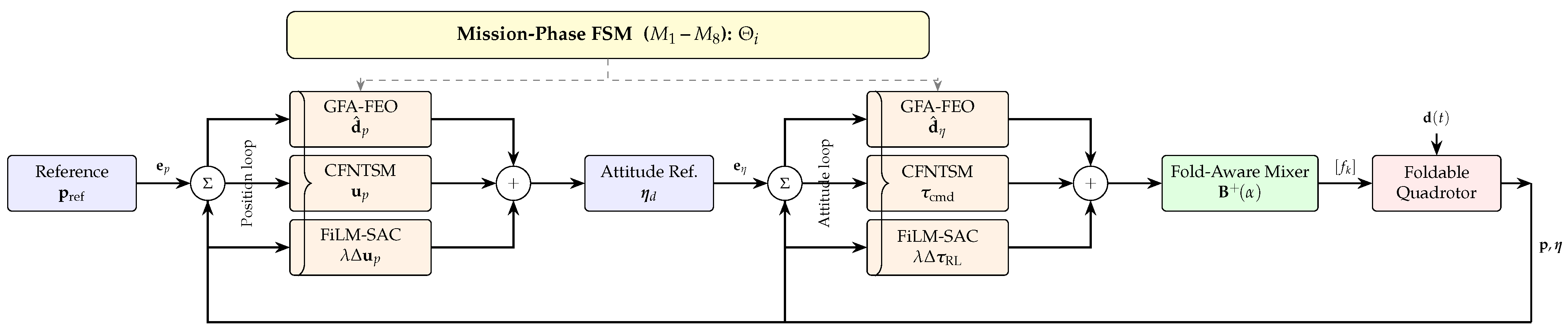
Within each loop, three complementary control layers operate in parallel (Figure 8): (1) a gait-frequency-aware finite-time extended observer (GFA-FEO) that cancels the dominant periodic disturbance at $f_g$ and its harmonics; (2) a continuous fast nonsingular terminal sliding-mode controller (CFNTSM) with $\alpha$-scheduled gains for broadband disturbance rejection and finite-time convergence; and (3) a FiLM-SAC residual RL policy conditioned on fold angle, gait parameters, and mission phase, with an adaptive trust weight $\lambda \left(t\right)$. A finite-state machine (FSM) orchestrates the mission by switching controller parameters, observer gains, and the RL trust weight across eight operational phases.

3.1. Controller Interaction and Coordination

The three controller components are coordinated as a parallel compensation structure under FSM supervision, rather than as independent methods that are activated in isolation. At each control step, the fold-angle-dependent plant model provides $\mathbf{g}\left(\alpha \right)$, $\mathbf{B}\left(\alpha \right)$, and $\mathbf{J}\left(\alpha \right)$ to both the CFNTSM law and the fold-aware allocation layer. The GFA-FEO estimates the lumped disturbance in the same standardised plant coordinates and passes $\hat{\mathbf{d}}$ to the CFNTSM law as a feedforward compensation term. CFNTSM then computes the stabilising nominal input, while the FiLM-SAC actor receives the tracking errors, observer residuals, fold state, gait estimate, and FSM phase and outputs only a bounded residual correction after the model-based input has been formed.

The FSM coordinates transitions by updating three quantities together: observer bandwidth and internal-model gains, CFNTSM gain-scheduling multipliers, and the residual-RL trust bound ${\overline{\lambda }}^{\left(M_i\right)}$. These updates are filtered or ramped at phase boundaries so that the commanded torque does not jump when the mission changes from approach to descent, docking, locking, stowing, or takeoff. Consequently, the model-based CFNTSM + GFA-FEO backbone remains active throughout the mission, while the learned residual is allowed to contribute mainly in phases where structured residual errors are expected, such as fold-through descent and the observer re-convergence window after EPM locking.

Figure 8 summarises this coordinated signal flow from reference generation through the GFA-FEO, CFNTSM, FiLM-SAC residual, fold-aware mixer, and folded-airframe plant.

3.2. Mission-Phase Finite-State Machine

The docking-and-takeoff mission is decomposed into eight sequential phases managed by a deterministic FSM. Each phase defines a distinct set of reference trajectories, controller gains, observer bandwidths, and RL trust-weight bounds.

Table 2. Mission-phase FSM: phases and transition conditions.

ID	Phase	Entry Condition
$M_1$	approach	Mission start; UAV airborne, $\parallel \mathbf{p}-{\mathbf{p}}_{\mathrm{dog}}\parallel >2$ m
$M_2$	align	$\parallel {\mathbf{p}}_{xy}-{\mathbf{p}}_{\mathrm{land},xy}\parallel <0.5$ m and $|z-z_{\mathrm{land}}|<1.0$ m
$M_3$	descend	Aligned: $\parallel \mathrm{\Delta }{\mathbf{p}}_{xy}\parallel <50$ mm; arms begin folding ($\dot{\alpha }<0$)
$M_4$	dock	Docking window: $\parallel \mathrm{\Delta }{\mathbf{p}}_{xy}\parallel <30$ mm, $\left|\mathrm{\Delta }\varphi \right|,\left|\mathrm{\Delta }\theta \right|<3^{°}$
$M_5$	lock	EPM activated; docking condition (22) satisfied
$M_6$	stow	Locked; arms fold to ${\alpha }_{\mathrm{fold}}$; motors idle
$M_7$	takeoff	Stow complete; takeoff command received
$M_8$	cruise	$z>z_{\mathrm{land}}+1.0$ m and $\parallel \dot{\mathbf{p}}\parallel <0.2$ m/s

lists all phases with their entry/exit conditions.

Each phase $M_i$ carries a parameter dictionary

$${\mathrm{\Theta }}_i=\left\{k_{1,p}^{\left(i\right)},k_{2,p}^{\left(i\right)},{\beta }_p^{\left(i\right)},k_{1,\eta }^{\left(i\right)},k_{2,\eta }^{\left(i\right)},{\beta }_{\eta }^{\left(i\right)},L_p^{\left(i\right)},L_{\eta }^{\left(i\right)},{\overline{\lambda }}^{\left(i\right)}\right\}$$

that is loaded upon entry and held constant within the phase. Here, the subscripts p and $\eta$ distinguish the position- and attitude-loop parameters, which are tuned independently (Section 4.1). Transitions between adjacent phases are irreversible in the nominal mission; an emergency abort returns to $M_1$.

Three phases deserve particular attention. During descend ($M_3$), the GFA-FEO switches to enhanced-gain mode (Section 3.4), the CFNTSM gains are boosted to compensate for moment-arm degradation during folding, and $\overline{\lambda }$ is elevated to allow larger residual-RL corrections. At lock ($M_5$), the RL trust weight is ramped to zero ($\lambda \to 0$) to prevent learned actions from disturbing the mechanical locking process. During takeoff ($M_7$), the FEO parameters have already been hot-switched at the $M_5\to M_6$ transition (Section 3.9) to accommodate the doubled mass; $\lambda$ is temporarily elevated, but remains bounded, to bridge the observer re-convergence blind window ($T_{\mathrm{blind}}\approx 0.2$–$0.3$ s). If the observer residual or tracking error does not decay after this window, the FSM holds the vehicle in a conservative vertical-climb mode and prevents further mission progression until the residual falls below threshold.

3.3. Standardised Plant Model

Both the position and attitude loops are expressed in a unified second-order form. Define the generalised state $\mathbf{x}\in \{\mathbf{p},\mathit{\eta }\}$ and the corresponding tracking error $\mathbf{e}=\mathbf{x}-{\mathbf{x}}_{\mathrm{ref}}$. The error dynamics are:

$$\ddot{\mathbf{e}}=\mathbf{f}(\mathbf{x},\dot{\mathbf{x}})+\mathbf{g}\left(\alpha \right)\mathbf{u}+\mathbf{d}\left(t\right),$$

(26)

where $\mathbf{u}$ is the control input, $\mathbf{g}\left(\alpha \right)$ is the fold-angle-dependent control-effectiveness matrix, and $\mathbf{d}\left(t\right)$ is the lumped disturbance satisfying $\parallel \mathbf{d}\parallel \le \overline{d}$ and $\parallel \dot{\mathbf{d}}\parallel \le {\overline{d}}_1$ (Assumption A3).

For the position loop, from (8) with ${\mathbf{e}}_p=\mathbf{p}-{\mathbf{p}}_{\mathrm{land}}$:

$${\ddot{\mathbf{e}}}_p={\displaystyle \frac{F}{m}}\mathbf{R}{\mathbf{e}}_3-g{\mathbf{e}}_3-{\ddot{\mathbf{p}}}_{\mathrm{land}}+{\displaystyle \frac{1}{m}}{\mathbf{d}}_{\mathrm{ext}},$$

(27)

where F is the total thrust, $\mathbf{R}$ the rotation matrix (5), and ${\ddot{\mathbf{p}}}_{\mathrm{land}}$ includes the gait-induced acceleration of the landing surface. The position-loop lumped disturbance is ${\mathbf{d}}_p=-{\ddot{\mathbf{p}}}_{\mathrm{land}}+{\mathbf{d}}_{\mathrm{ext}}/m+(K_{\mathrm{GE}}-1)F\mathbf{R}{\mathbf{e}}_3/m$, incorporating the reference acceleration, external wind, and ground-effect residual.

For the attitude loop, from (9) with ${\mathbf{e}}_{\eta }=\mathit{\eta }-{\mathit{\eta }}_d$ (where ${\mathit{\eta }}_d$ comes from the outer loop):

$${\ddot{\mathbf{e}}}_{\eta }={\mathbf{J}}^{-1}\left(\alpha \right)\left[-\mathit{\omega }\times \mathbf{J}\left(\alpha \right)\mathit{\omega }+\mathbf{B}\left(\alpha \right)\mathbf{f}+{\mathbf{\tau }}_G+{\mathbf{\tau }}_D+{\mathbf{\tau }}_{\mathrm{ext}}\right]-{\ddot{\mathit{\eta }}}_d.$$

(28)

Here the control-effectiveness matrix is ${\mathbf{g}}_{\eta }\left(\alpha \right)={\mathbf{J}}^{-1}\left(\alpha \right)\mathbf{B}\left(\alpha \right)$, which varies continuously with the fold angle and becomes asymmetric in the folded state (Section 2.2.2). The attitude-loop lumped disturbance is ${\mathbf{d}}_{\eta }={\mathbf{J}}^{-1}[-\mathit{\omega }\times \mathbf{J}\mathit{\omega }+{\mathbf{\tau }}_G+{\mathbf{\tau }}_D+{\mathbf{\tau }}_{\mathrm{ext}}]-{\ddot{\mathit{\eta }}}_d$.

Unlike conventional quadrotor models where $\mathbf{g}$ is a constant diagonal matrix, ${\mathbf{g}}_{\eta }\left(\alpha \right)={\mathbf{J}}^{-1}\left(\alpha \right)\mathbf{B}\left(\alpha \right)$ varies with $\alpha$ and is non-diagonal in the folded state due to the asymmetric moment arms. This $\alpha$-dependence propagates to gain scheduling (Section 3.5) and the allocation inverse (Section 3.6).

3.4. Gait-Frequency-Aware Finite-Time Extended Observer

The GFA-FEO is designed to estimate the lumped disturbance $\mathbf{d}\left(t\right)$ in (26) with two key enhancements over a standard finite-time extended observer: (i) a periodic internal-model term tuned to the gait frequency $f_g$ and its harmonics, and (ii) an enhanced-gain mode activated during the descend phase.

3.4.1. Observer Structure

Consider the standardised plant (26) with state vector ${[\mathbf{e},\dot{\mathbf{e}},\mathbf{d}]}^T$. The GFA-FEO introduces observer states $[\hat{\mathbf{e}},\widehat{\dot{\mathbf{e}}},\hat{\mathbf{d}}]$ and estimation errors ${\tilde{\mathbf{e}}}_i={\widehat{(·)}}_i-{(·)}_i$:

$$\begin{array}{cc}\hfill \dot{\hat{\mathbf{e}}}& =\widehat{\dot{\mathbf{e}}}-{\ell }_{1}L{\lceil \tilde{\mathbf{e}}\rfloor }^{1-{\epsilon }_1},\hfill \\ \hfill \dot{\widehat{\dot{\mathbf{e}}}}& =\mathbf{g}\left(\alpha \right)\mathbf{u}+\hat{\mathbf{d}}+{\hat{\mathbf{d}}}_{\mathrm{IM}}-{\ell }_2{L}^2{\lceil \tilde{\mathbf{e}}\rfloor }^{1-2{\epsilon }_1}+{\widehat{\dot{\mathbf{e}}}}_{\mathrm{vel}},\hfill \\ \hfill \dot{\hat{\mathbf{d}}}& =-{\ell }_3{L}^3{\lceil \tilde{\mathbf{e}}\rfloor }^{1-3{\epsilon }_1}+{\hat{\mathbf{d}}}_{\mathrm{IM}},\hfill \end{array}$$

(29)

where ${\lceil ·\rfloor }^{\gamma }$ denotes the signed fractional power ${\lceil x\rfloor }^{\gamma }={\left|x\right|}^{\gamma }sign\left(x\right)$, $L>0$ is the observer bandwidth (tuned separately for the position and attitude loops as $L_{\mathrm{pos}}$ and $L_{\mathrm{att}}$ to account for their different noise environments and disturbance spectra), ${\ell }_1,{\ell }_2,{\ell }_3>0$ are design gains, and ${\epsilon }_1\in (0,1/2)$ is the fractional exponent satisfying the finite-time convergence condition [43]. The combined disturbance estimate $\hat{\mathbf{d}}+{\hat{\mathbf{d}}}_{\mathrm{IM}}$ is clamped to $[-{\hat{d}}_{max},{\hat{d}}_{max}]$ per channel, where ${\hat{d}}_{max}>0$ is a saturation bound that prevents transient over-compensation during observer initialisation or sudden disturbance transitions.

The velocity-error correction term ${\widehat{\dot{\mathbf{e}}}}_{\mathrm{vel}}$ exploits the measured velocity (from state estimation or optical flow) to accelerate convergence:

$${\widehat{\dot{\mathbf{e}}}}_{\mathrm{vel}}=-{\mu }_v(\widehat{\dot{\mathbf{e}}}-{\dot{\mathbf{e}}}_{\mathrm{meas}}),{\mu }_v>0.$$

(30)

Both the position and velocity measurements fed to the observer are first passed through a discrete first-order low-pass filter $y_k={\alpha }_f{x}_k+(1-{\alpha }_f)y_{k-1}$, where ${\alpha }_f=\mathrm{\Delta }t/(\mathrm{\Delta }t+1/\left(2\pi f_c\right))$. The position-channel cutoff is $f_{c,p}=30$ Hz and the velocity-channel cutoff is $f_{c,v}=60$ Hz, chosen to attenuate sensor noise above the gait-harmonic band ($2f_g=5$ Hz) while preserving sufficient phase margin for the observer and control loops.

3.4.2. Gait-Frequency Internal Model

A standard FEO treats the disturbance as wideband and estimates it through high-gain injection. However, the gait-induced disturbance is dominated by three narrow-band components at $f_g/2$, $f_g$, and $2f_g$ (Section 2.4). A wideband observer achieves zero steady-state error only for constant disturbances; for sinusoidal signals at frequency ${\omega }_n$, a phase lag $\propto {\omega }_n/L$ persists unless an internal model at that frequency is embedded.

The internal-model augmentation generates a feedforward correction in the disturbance channel:

$${\hat{\mathbf{d}}}_{\mathrm{IM}}=\sum _{n\in \mathcal{H}}\left[{\mathbf{a}}_{n}sin\left(2\pi n{f}_{g}t\right)+{\mathbf{b}}_{n}cos\left(2\pi n{f}_{g}t\right)\right],$$

(31)

where $\mathcal{H}=\{\frac{1}{2},1,2\}$ indexes the three gait harmonics. The Fourier coefficients ${\mathbf{a}}_n,{\mathbf{b}}_n$ are adapted online via:

$${\dot{\mathbf{a}}}_n=-{\gamma }_n\tilde{\mathbf{e}}sin\left(2\pi n{f}_{g}t\right)-{\sigma }_{\mathrm{IM}}{\mathbf{a}}_n,{\dot{\mathbf{b}}}_n=-{\gamma }_n\tilde{\mathbf{e}}cos\left(2\pi n{f}_{g}t\right)-{\sigma }_{\mathrm{IM}}{\mathbf{b}}_n,$$

(32)

with adaptation rate ${\gamma }_n>0$. The $\sigma$-modification terms $-{\sigma }_{\mathrm{IM}}{\mathbf{a}}_n$ and $-{\sigma }_{\mathrm{IM}}{\mathbf{b}}_n$ (${\sigma }_{\mathrm{IM}}>0$ small) provide a leakage that prevents unbounded growth of the Fourier coefficients when the gait frequency drifts or the observer operates in transient conditions, at the cost of a small steady-state bias that is negligible for ${\sigma }_{\mathrm{IM}}\ll {\gamma }_n$. By the internal-model principle, the closed-loop observer achieves exact asymptotic cancellation of the gait-periodic component, regardless of the observer bandwidth L—a property unattainable by the standard FEO alone.

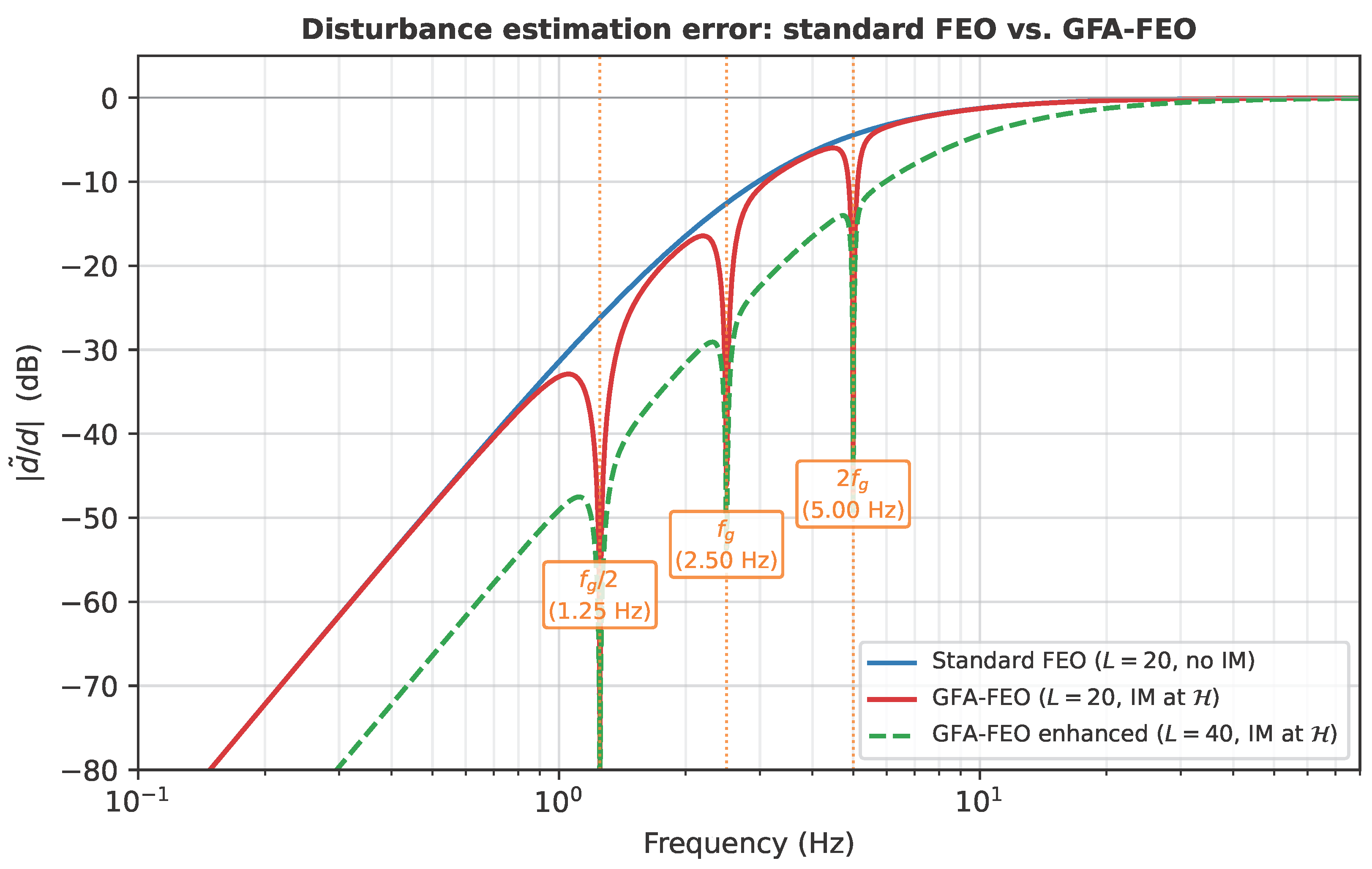
Figure 9 compares the disturbance estimation error $|\tilde{d}/d|\left(j\omega \right)$ for the standard FEO and the proposed GFA-FEO. The internal-model terms create deep notches at $f_g/2$, $f_g$, and $2f_g$ (the three dominant gait harmonics), reducing the estimation error by over 30 dB relative to the standard observer at those frequencies. In enhanced-gain mode ($L^{\left(M_3\right)}=2L$), the entire curve shifts downward, further improving broadband disturbance rejection during the critical descent phase.

When the gait frequency is not known a priori (e.g., the robot changes speed), $f_g$ is estimated from the dog-frame IMU by peak detection on the pitch-rate spectrum and communicated to the UAV at 10 Hz.

3.4.3. Enhanced-Gain Mode

The observer must be more aggressive during terminal descent than during approach because the landing surface motion is both closer and more consequential: a few millimetres of phase lag can decide whether the EPM array enters the capture window. Enhanced-gain mode is thus implemented as an FSM-triggered temporary increase in observer bandwidth and internal-model adaptation, rather than as a globally large gain that would amplify noise throughout the mission.

During the descend phase ($M_3$), the UAV approaches the vibrating surface, and the gait-induced disturbance amplitude grows. Simultaneously, the arm folding degrades moment arms, reducing the disturbance-rejection bandwidth. To counteract both effects, the FSM triggers an enhanced-gain mode:

$$L^{\left(M_3\right)}={\kappa }_L{L}^{\left(M_2\right)},{\gamma }_n^{\left(M_3\right)}={\kappa }_{\gamma }{\gamma }_n^{\left(M_2\right)},$$

(33)

where ${\kappa }_L>1$ and ${\kappa }_{\gamma }>1$ are boost factors. The transition is smoothed by a first-order filter $L\left(t\right)=L^{\left(M_2\right)}+(L^{\left(M_3\right)}-L^{\left(M_2\right)})(1-e^{-t/{\tau }_L})$ to avoid observer transients.

3.4.4. GFA-FEO Convergence

Theorem 1. 

Consider the standardised plant (26) with bounded disturbance $\parallel \dot{\mathbf{d}}\parallel \le {\overline{d}}_1$. The GFA-FEO (29)–(32) guarantees that the observation errors $\tilde{\mathbf{e}}$, $\widetilde{\dot{\mathbf{e}}}$, and $\tilde{\mathbf{d}}$ converge to a neighbourhood of the origin in finite time $T_{\mathrm{obs}}$. Furthermore, the steady-state disturbance estimation error for any component at frequency $n{f}_g$, $n\in \mathcal{H}$, satisfies $\parallel {\tilde{\mathbf{d}}}_{n{f}_g}\parallel \to 0$ as $t\to \infty$.

Proof. 

Define the scaled estimation errors ${\mathbf{\xi }}_1=L^{-1}\tilde{\mathbf{e}}$, ${\mathbf{\xi }}_2=L^{-2}\widetilde{\dot{\mathbf{e}}}$, ${\mathbf{\xi }}_3=L^{-3}\tilde{\mathbf{d}}$. Under the coordinate transformation, the error dynamics become:

$${\dot{\mathbf{\xi }}}_i=L\left[{\mathbf{\xi }}_{i+1}-{\ell }_i{\lceil {\mathbf{\xi }}_1\rfloor }^{1-i{\epsilon }_1}\right]+{\mathit{\delta }}_i,i=1,2,$$

(34)

with ${\mathbf{\xi }}_4=\mathbf{0}$ and ${\mathit{\delta }}_i$ containing the internal-model terms and $\dot{\mathbf{d}}/L^3$. Consider the Lyapunov function:

$$V_{\mathrm{obs}}={\displaystyle \sum _{i=1}^3}\frac{1}{2}{\mathbf{\xi }}_i^T{\mathbf{\xi }}_i.$$

(35)

Its time derivative satisfies (following the homogeneous-domination approach of [43]):

$${\dot{V}}_{\mathrm{obs}}\le -c_{1}L{V}_{\mathrm{obs}}^{1-{\epsilon }_1/2}+c_2{\displaystyle \frac{{\overline{d}}_1}{L^3}},$$

(36)

where $c_1,c_2>0$ depend on ${\ell }_1,{\ell }_2,{\ell }_3$. For sufficiently large L, the first term dominates, yielding finite-time convergence to the ball $\parallel \mathbf{\xi }\parallel \le {(c_2{\overline{d}}_1/\left(c_1{L}^4\right))}^{1/(2-{\epsilon }_1)}$.

For the periodic component, the analysis proceeds in the regime $t>T_{\mathrm{obs}}$ where $\parallel \tilde{\mathbf{e}}\parallel \le \overline{\xi }$ is already small. Define ${\tilde{\mathbf{a}}}_n={\hat{\mathbf{a}}}_n-{\mathbf{a}}_n^{\ast }$, ${\tilde{\mathbf{b}}}_n={\hat{\mathbf{b}}}_n-{\mathbf{b}}_n^{\ast }$ where ${\mathbf{a}}_n^{\ast },{\mathbf{b}}_n^{\ast }$ are the true Fourier coefficients. Consider the augmented Lyapunov function $V_{\mathrm{IM}}={\sum }_n{\displaystyle \frac{1}{2{\gamma }_n}}({\parallel {\tilde{\mathbf{a}}}_n\parallel }^2+{\parallel {\tilde{\mathbf{b}}}_n\parallel }^2)$. Substituting the adaptation law (32):

$${\dot{V}}_{\mathrm{IM}}=-\sum _n{\tilde{\mathbf{a}}}_n^T\tilde{\mathbf{e}}sin\left(2\pi n{f}_{g}t\right)-\sum _n{\tilde{\mathbf{b}}}_n^T\tilde{\mathbf{e}}cos\left(2\pi n{f}_{g}t\right).$$

(37)

The gait frequencies $\{n{f}_g:n\in \mathcal{H}\}$ are distinct and non-resonant, so the sinusoidal regressors are persistently exciting. By the Barbalat–LaSalle argument (the integrand is uniformly continuous and the integral is bounded), ${\tilde{\mathbf{a}}}_n$ and ${\tilde{\mathbf{b}}}_n$ converge to zero as $t\to \infty$, guaranteeing complete cancellation of the gait-periodic disturbance.    □

3.5. $\alpha$-Scheduled CFNTSM Controller

The observer of Section 3.3 provides disturbance estimates, while the tracking law must preserve authority as folding reduces the rotor moment arms. The controller therefore combines a thrust–attitude cascade, a nonsingular terminal sliding surface, fold-angle gain scheduling, and a fold-aware control law.

3.5.1. Cascade Connection: Thrust–Attitude Extraction

The position-loop CFNTSM computes a desired inertial-frame acceleration ${\mathbf{a}}_{\mathrm{cmd}}\in {\mathbb{R}}^3$ (see (43) below); adding the gait-acceleration feedforward yields the total commanded acceleration $\mathbf{a}={\mathbf{a}}_{\mathrm{cmd}}+{\ddot{\mathbf{p}}}_{\mathrm{land}}$. To compensate for the phase delay introduced by the first-order motor dynamics (${\tau }_m=20$ ms), the gait-acceleration feedforward ${\ddot{\mathbf{p}}}_{\mathrm{land}}$ is evaluated at the phase-advanced time $t+{\tau }_m$ rather than the current time t, i.e., ${\ddot{\mathbf{p}}}_{\mathrm{land}}\left(t\right)\leftarrow {\ddot{\mathbf{p}}}_{\mathrm{land}}(t+{\tau }_m)$. This predictive shift reduces the steady-state vertical tracking bias caused by the lag between desired and realised thrust. The desired thrust magnitude and body-frame attitude are extracted via the standard differential-flatness relations:

$$\begin{array}{cc}\hfill F_{\mathrm{cmd}}& =m\sqrt{a_x^2+a_y^2+{(a_z+g)}^2},\hfill \\ \hfill {\varphi }_{\mathrm{des}}& =arctan2\left(a_{y,b},a_z+g\right),\hfill \\ \hfill {\theta }_{\mathrm{des}}& =arctan2\left(a_{x,b},\sqrt{a_{y,b}^2+{(a_z+g)}^2}\right),\hfill \end{array}$$

(38)

where $a_{x,b}=a_{x}cos\psi +a_{y}sin\psi$ and $a_{y,b}=a_{x}sin\psi -a_{y}cos\psi$ are the yaw-rotated horizontal acceleration components. The desired Euler angles fed to the inner loop are then ${\mathit{\eta }}_d={[{\varphi }_{\mathrm{des}}+{\varphi }_{\mathrm{gait}},{\theta }_{\mathrm{des}}+{\theta }_{\mathrm{gait}},{\psi }_d]}^T$, where ${\varphi }_{\mathrm{gait}},{\theta }_{\mathrm{gait}}$ are the gait-induced body-roll and pitch of the landing platform.

The inner-loop angular-velocity reference is ${\mathit{\omega }}_{\mathrm{ref}}=\mathbf{W}\left({\mathit{\eta }}_d\right){\dot{\mathit{\eta }}}_d$, where $\mathbf{W}$ is the Euler-to-body-rate Jacobian and ${\dot{\mathit{\eta }}}_d$ denotes the total rate of change of ${\mathit{\eta }}_d$—including both the gait-rate contribution and the rate generated by the outer-loop acceleration command (obtained via numerical differentiation at the control rate, low-pass clipped at ±20 rad/s to prevent derivative spikes).

The sliding surface combines position or attitude error with a nonsingular terminal term in the error derivative. This choice keeps the finite-time convergence property of terminal sliding mode control while avoiding the singularity that would otherwise appear when ${\dot{e}}_j$ approaches zero.

For each control channel of (26), the continuous fast nonsingular terminal sliding-mode (CFNTSM) surface is defined as:

$$s_j=e_j+{\beta }_j{\lceil {\dot{e}}_j\rfloor }^{p_j/q_j},j\in \{x,y,z,\varphi ,\theta ,\psi \},$$

(39)

where ${\beta }_j>0$ is the surface parameter, and $p_j,q_j$ are positive odd integers satisfying $1<p_j/q_j<2$ to ensure nonsingularity of the control law when ${\dot{e}}_j=0$.

3.5.2. Fold-Angle-Dependent Gain Scheduling

As $\alpha$ decreases from ${45}^{°}$ (deployed) to $-{76.5}^{°}$ (folded), the effective moment arms shrink significantly (Section 2.2.2). If the controller gains remain fixed, the closed-loop bandwidth degrades proportionally, potentially destabilising the attitude loop in the folded state.

To compensate, the CFNTSM gains are scheduled as functions of the second singular value of the torque allocation matrix $\mathbf{B}\in {\mathbb{R}}^{3\times 4}$:

$$k_{1,j}\left(\alpha \right)=k_{1,j}^{\mathrm{nom}}·{\displaystyle \frac{{\sigma }_2\left({\mathbf{B}}_{\mathrm{dep}}\right)}{{\sigma }_2\left(\mathbf{B}\left(\alpha \right)\right)+{ϵ}_{\sigma }}},k_{2,j}\left(\alpha \right)=k_{2,j}^{\mathrm{nom}}·{\displaystyle \frac{{\sigma }_2\left({\mathbf{B}}_{\mathrm{dep}}\right)}{{\sigma }_2\left(\mathbf{B}\left(\alpha \right)\right)+{ϵ}_{\sigma }}},$$

(40)

where $k_{1,j}^{\mathrm{nom}},k_{2,j}^{\mathrm{nom}}$ are the nominal gains tuned for the deployed configuration, ${\sigma }_2\left({\mathbf{B}}_{\mathrm{dep}}\right)$ is the second singular value of the deployed allocation matrix (a constant reference that normalises the scheduling ratio to unity at $\alpha ={45}^{°}$), ${\sigma }_2\left(\mathbf{B}\left(\alpha \right)\right)$ is the current second singular value (computed in real time from the known $\alpha$), and ${ϵ}_{\sigma }>0$ is a small regularisation constant preventing division by zero at hypothetical rank-deficient configurations. The second singular value is chosen instead of the minimum (${\sigma }_3$) because ${\sigma }_3$ is dominated by the yaw channel (whose moment arm is an order of magnitude smaller than roll/pitch), and scheduling on ${\sigma }_3$ would yield excessively large gain ratios that destabilise the roll/pitch loops.

This scheduling ensures that the effective control authority experienced by the sliding-mode controller remains approximately constant across the entire fold range: as the physical moment arms shrink, the gains increase to maintain the same closed-loop bandwidth.

The regularisation constant ${ϵ}_{\sigma }$ also sets the practical trade-off between convergence speed and control-input limits. The nonsingular terminal surface itself is shaped by the exponent $p_j/q_j$ in (39); the small “epsilon” used in the CFNTSM implementation is the gain-scheduling regulariser ${ϵ}_{\sigma }$, distinct from the observer exponent ${\epsilon }_1$ and the ultimate-bound radius ${ϵ}_s$ in the stability proof. From (40), the scheduled gains are upper-bounded by $k_{1,j}^{max}=k_{1,j}^{\mathrm{nom}}{\sigma }_2\left({\mathbf{B}}_{\mathrm{dep}}\right)/{ϵ}_{\sigma }$ and analogously for $k_{2,j}$. A smaller ${ϵ}_{\sigma }$, therefore, increases $k_{1,j}$ and $k_{2,j}$ when the folded configuration makes ${\sigma }_2\left(\mathbf{B}\left(\alpha \right)\right)$ small, which increases the finite-time convergence coefficient in (55) and reduces settling time. The cost is a larger requested $u_{\mathrm{CFNTSM},j}$ and a higher risk of motor-thrust clipping, noise amplification, or chattering near rank-deficient configurations. Conversely, a larger ${ϵ}_{\sigma }$ softens the gain amplification and keeps the allocated thrusts farther from actuator limits, but it slows the terminal convergence and leaves a larger residual error during fold-through descent. In implementation, ${ϵ}_{\sigma }$ is chosen so that the scheduled gains at $\alpha =-{76.5}^{°}$ remain compatible with the damped pseudo-inverse allocation and the motor thrust bounds; the condition-number warning and thrust clipping in Section 3.6 provide the final input-limit safeguards.

Because the gait-induced disturbance amplitude grows with frequency, the gain-scheduling ratio is tuned at the nominal $f_g^{\mathrm{nom}}=2.5$ Hz can be overly aggressive at lower gait frequencies where less compensatory authority is needed. To prevent this, the reference singular value is scaled by a frequency-dependent factor:

$${\sigma }_2^{\mathrm{eff}}={\sigma }_2\left({\mathbf{B}}_{\mathrm{dep}}\right)·min\left(1,{\displaystyle \frac{f_g}{f_g^{\mathrm{nom}}}}\right),$$

(41)

so that (40) becomes $k_{1,j}(\alpha ,f_g)=k_{1,j}^{\mathrm{nom}}{\sigma }_2^{\mathrm{eff}}/[{\sigma }_2\left(\mathbf{B}\left(\alpha \right)\right)+{ϵ}_{\sigma }]$. At $f_g=f_g^{\mathrm{nom}}$ the factor is unity and the original schedule is recovered; at lower frequencies the effective ceiling is reduced proportionally, preventing over-amplified gains from degrading precision.

Additionally, the FSM applies a phase-specific multiplier:

$$k_j^{\left(M_i\right)}\left(\alpha \right)={\zeta }^{\left(M_i\right)}·k_j\left(\alpha \right),$$

(42)

where ${\zeta }^{\left(M_i\right)}\ge 1$ is a phase boost factor (e.g., ${\zeta }^{\left(M_3\right)}>1$ during descend for tighter tracking near the vibrating surface).

3.5.3. Control Law

The control input combines three terms: cancellation of the known channel dynamics, compensation of the GFA-FEO disturbance estimate, and finite-time feedback on the sliding variable. Written per standardised channel, the CFNTSM law is

$$u_{\mathrm{CFNTSM},j}=-g_j^{-1}\left(\alpha \right)\left[f_j+{\hat{d}}_j+{\displaystyle \frac{q_j}{p_j{\beta }_j}}{\left|{\dot{e}}_j\right|}^{2-p_j/q_j}sign\left({\dot{e}}_j\right)+k_{1,j}\left(\alpha \right){\lceil s_j\rfloor }^{{\rho }_1}+k_{2,j}\left(\alpha \right)s_j\right],$$

(43)

where ${\hat{d}}_j$ is the GFA-FEO estimate from (29), $f_j$ is the known drift term, and ${\rho }_1\in (0,1)$ provides the finite-time convergence characteristic. For the position loop, $f_j=0$ because the gravity term is absorbed into the thrust–attitude extraction (38). For the attitude loop, the known drift is the gyroscopic coupling

$$f_j={\left[{\mathbf{J}}^{-1}\left(\alpha \right)\left(-\mathit{\omega }\times \mathbf{J}\left(\alpha \right)\mathit{\omega }\right)\right]}_j,$$

(44)

which is computable in real time from the measured angular velocity and the known inertia tensor. The remaining nonlinear terms (drag torques ${\mathbf{\tau }}_D$, gravity torques ${\mathbf{\tau }}_G$, external disturbances ${\mathbf{\tau }}_{\mathrm{ext}}$, and the reference acceleration $-{\ddot{\mathit{\eta }}}_d$) are absorbed into ${\mathbf{d}}_{\eta }$ and estimated by the GFA-FEO.

The term $g_j^{-1}\left(\alpha \right)$ cancels the fold-dependent control effectiveness; combined with the gain scheduling (40), this constitutes a double compensation for the moment-arm degradation—cancellation in the plant model and gain amplification for disturbance rejection.

Remark (non-diagonal attitude effectiveness). For the position loop, $g_j\left(\alpha \right)$ is the scalar thrust-to-force effectiveness for each translational channel. For the attitude loop, $g_j\left(\alpha \right)$ denotes the j-th diagonal element of ${\mathbf{g}}_{\eta }\left(\alpha \right)={\mathbf{J}}^{-1}\left(\alpha \right)\mathbf{B}\left(\alpha \right)$. As noted in Section 3.3, this matrix becomes non-diagonal in the folded state. The off-diagonal coupling terms are treated as part of the lumped disturbance ${\mathbf{d}}_{\eta }$ under Assumption A3 and estimated by the GFA-FEO. This approximation is valid provided the off-diagonal entries remain smaller than the minimum diagonal gain, a condition satisfied in hardware for $\alpha \ge -{76.5}^{°}$ (verified numerically in Section 5).

3.5.4. Continuity at FSM Transitions

The FSM changes controller gains at phase boundaries; for example, when the controller switches from approach to descent or from docking to takeoff. Although these changes are physically motivated, applying them as instantaneous steps would inject artificial torque spikes into the allocation layer. The smoothing rule below preserves the intended phase-dependent gains while making the commanded input continuous.

When the FSM transitions from phase $M_i$ to $M_{i+1}$, the gain parameters $k_j$ change discontinuously. To avoid control chattering, a first-order exponential filter smooths the transition:

$$k_j\left(t\right)=k_j^{\left(M_i\right)}+\left(k_j^{\left(M_{i+1}\right)}-k_j^{\left(M_i\right)}\right)\left(1-e^{-(t-t_{\mathrm{sw}})/{\tau }_{\mathrm{sw}}}\right),$$

(45)

where $t_{\mathrm{sw}}$ is the switching instant and ${\tau }_{\mathrm{sw}}>0$ is the smoothing time constant (typically 50–100 ms).

3.6. Fold-Aware Control Allocation

The CFNTSM attitude controller outputs a desired torque vector ${\mathbf{\tau }}_{\mathrm{cmd}}\in {\mathbb{R}}^3$ (roll, pitch, and yaw). Together with the desired total thrust $F_{\mathrm{cmd}}$ from the position loop, the full allocation problem is

$$\underset{\mathbf{M}\left(\alpha \right)\in {\mathbb{R}}^{4\times 4}}{\underbrace{\left[\begin{array}{cccc}1& 1& 1& 1\\ & \mathbf{B}\left(\alpha \right)& & \end{array}\right]}}\left[\begin{array}{c}{f}_1\\ f_2\\ f_3\\ f_4\end{array}\right]=\left[\begin{array}{c}{F}_{\mathrm{cmd}}\\ {\mathbf{\tau }}_{\mathrm{cmd}}\end{array}\right].$$

(46)

In the deployed X-configuration, $\mathbf{M}$ is well-conditioned and its inverse is the classical symmetric mixer. As $\alpha$ decreases, $\mathbf{M}\left(\alpha \right)$ becomes progressively ill-conditioned: the minimum singular value drops from $\underline{\sigma }=0.116$ at $\alpha ={45}^{°}$ to $\underline{\sigma }=0.055$ at $\alpha =-{76.5}^{°}$.

The fold-aware allocation computes the motor thrusts via the damped pseudo-inverse

$$\mathbf{f}={\mathbf{M}}^T\left(\alpha \right){\left[\mathbf{M}\left(\alpha \right){\mathbf{M}}^T\left(\alpha \right)+{\delta }^2{\mathbf{I}}_4\right]}^{-1}\left[\begin{array}{c}{F}_{\mathrm{cmd}}\\ {\mathbf{\tau }}_{\mathrm{cmd}}\end{array}\right],$$

(47)

where $\delta >0$ is a damping factor that prevents numerical blow-up near rank deficiency. The result is clipped to the feasible thrust range $f_k\in [0,f_{max}]$.

At each control step, $\underline{\sigma }\left(\mathbf{M}\left(\alpha \right)\right)$ is computed and compared against a threshold ${\sigma }_{\mathrm{warn}}$. If $\underline{\sigma }<{\sigma }_{\mathrm{warn}}$, the controller limits the demanded torque magnitude to prevent actuator saturation, and a warning flag is set in the FSM.

3.7. Model-Based Performance Ceiling Analysis

Before introducing the learned residual layer, it is instructive to characterise the architectural performance limit of the model-based controller alone—i.e., the best tracking accuracy attainable by CFNTSM + GFA-FEO regardless of parameter tuning.

To quantify this ceiling, we conducted an exhaustive multi-phase parameter sweep (over 200 configurations) covering the CFNTSM gains $(k_1,k_2,\beta ,p/q,{\rho }_1)$, the GFA-FEO bandwidth and internal-model gains $({\ell }_i,L,{\epsilon }_1,{\gamma }_n,{\mu }_v)$, and the measurement LPF cutoffs $(f_{c,p},f_{c,v})$. Each configuration was evaluated under the nominal docking scenario ($v_d=0.5$ m/s, $f_g=2.5$ Hz, $v_w=2$ m/s) with 10 independent random seeds.

3.7.1. Bottleneck Identification

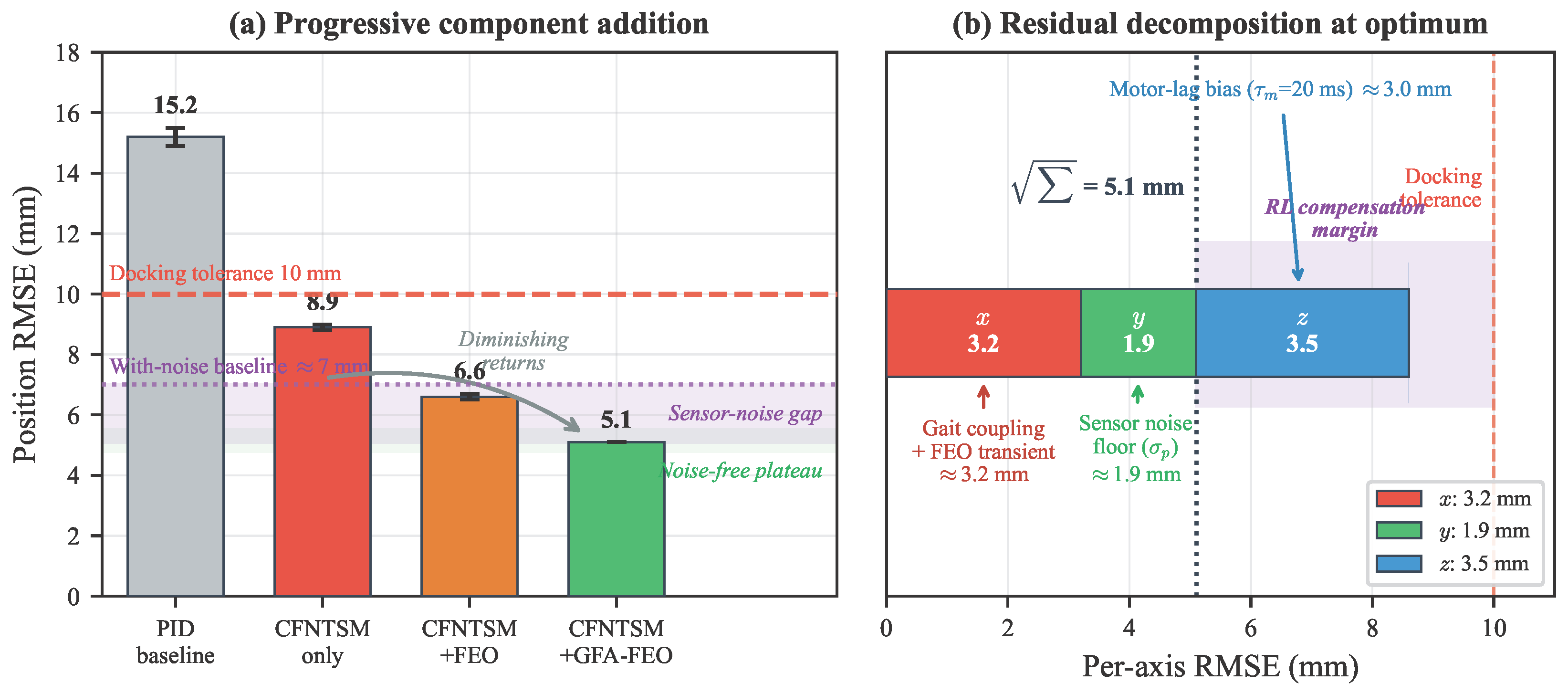
The ceiling analysis has two key findings. First, each successive model-based enhancement yields diminishing returns: the gap from PID to CFNTSM is 6.3 mm, from CFNTSM to +FEO is 2.3 mm, and from +FEO to +GFA-FEO is 1.5 mm. The position RMSE converges to a plateau around 5.1 mm despite exhaustive tuning of all available degrees of freedom.

The representative values supporting this comparison are summarised in

Table 3. Model-based performance ceiling: position RMSE under progressive component addition (10-seed average, nominal docking scenario, and noise-free evaluation). All configurations use PSO-optimised parameters.

Configuration	${\overline{\mathit{e}}}_{\mathit{p}}$ (mm)	${\mathit{e}}_{\mathit{x}}$ (mm)	${\mathit{e}}_{\mathit{y}}$ (mm)	${\mathit{e}}_{\mathit{z}}$ (mm)	${\overline{\mathit{z}}}_{\mathbf{bias}}$ (mm)	${\overline{\mathit{e}}}_{\mathit{\eta }}$ (°)
PID baseline	15.2 ± 0.3	—	—	—	—	3.8
CFNTSM only	8.9 ± 0.1	4.8	2.5	7.0	$-7.0$	2.0
CFNTSM + FEO (no IM)	6.6 ± 0.1	3.5	2.0	5.2	$-4.8$	2.2
CFNTSM + GFA-FEO	5.1 ± 0.0	3.2	1.9	3.5	$-3.0$	2.4

Note: Bold indicates the best value for the primary position-RMSE metric.

.

Figure 10 visualises the same performance ceiling and decomposes the residual error sources at the model-based optimum.

Panel (b) decomposes the residual error at the optimum into per-axis contributions. The z-axis component (3.5 mm) is dominated by a ≈ 3.0 mm steady-state bias from the motor time constant ${\tau }_m$; the phase-advance feedforward compensates the dominant harmonic, but the nonlinear interaction between fold-angle-dependent thrust effectiveness and the first-order motor lag leaves a residual beyond linear phase compensation. The x-axis component (3.2 mm) is driven by gait-coupled lateral disturbance at the walking frequency and the GFA-FEO finite-time transient during frequency lock-in. The y-axis component (1.9 mm) approaches the sensor noise floor (${\sigma }_p=0.5$ mm per sample, amplified by differentiation in the velocity channel).

3.7.2. Implication: Necessity of Learned Residual Compensation

The 5.1 mm plateau establishes the noise-free architectural limit of the model-based controller. When measurement noise is included (${\sigma }_p=0.5$ mm per position channel, amplified by differentiation in the velocity feedback path), the effective baseline RMSE rises to approximately 7 mm in the nominal scenario—still within the < 10 mm docking tolerance (22), but leaving limited margin under more challenging conditions (higher $f_g$, stronger wind). The remaining structured error stems from three sources that resist analytical cancellation: (i) the nonlinear coupling between fold-angle-dependent dynamics and motor lag, (ii) the finite convergence time of the FEO during transient disturbances, and (iii) sensor noise amplification in the velocity feedback path.

A learned residual policy, operating on the rich observation vector $\mathbf{o}$ conditioned on the fold angle $\alpha$ and FSM phase, can compensate for these structured residuals through nonlinear function approximation—particularly the sensor-noise-induced gap between the 5.1 mm noise-free limit and the ∼7 mm with-noise performance—and improve robustness across the operational envelope.

3.8. FiLM-SAC Residual Reinforcement Learning

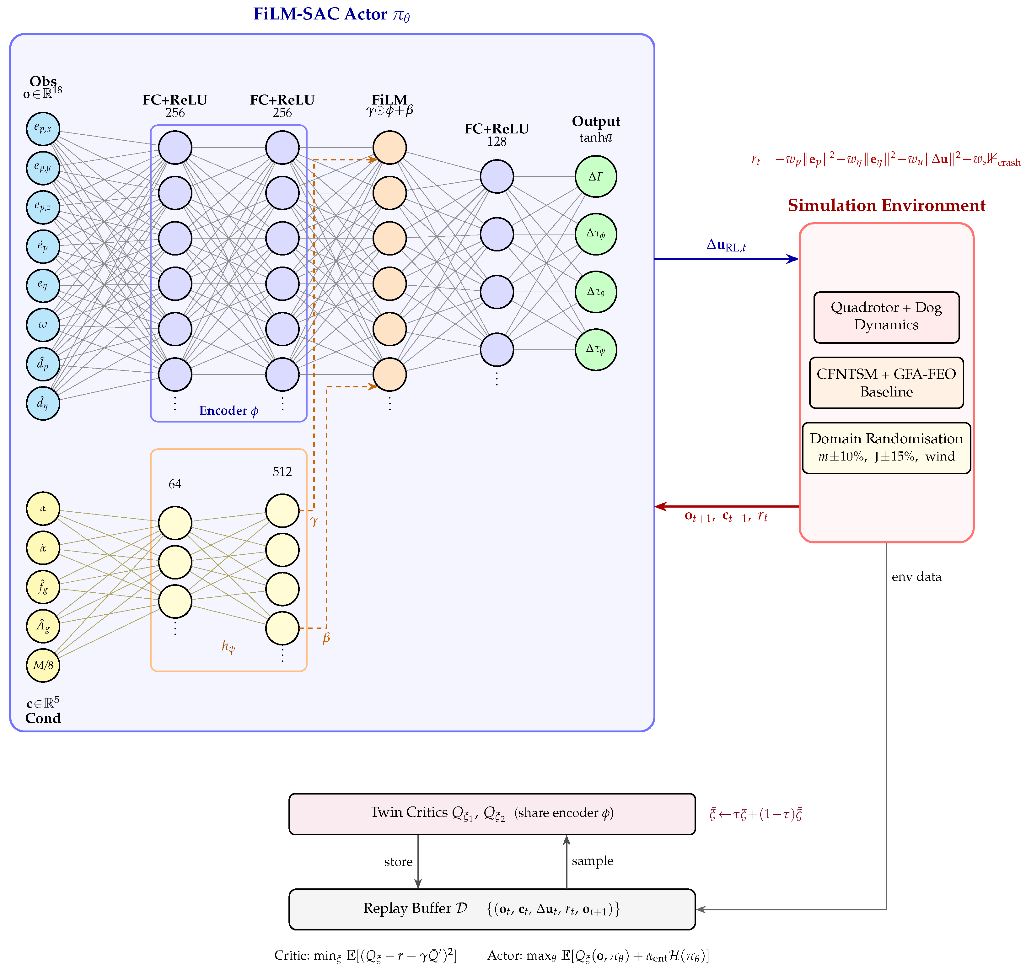
The model-based controller leaves a small but structured residual tracking error near the docking tolerance. The FiLM-SAC layer is introduced as a bounded residual compensator that can adapt its action to the fold state, gait estimate, and FSM phase while leaving the CFNTSM–GFA-FEO controller as the stabilising backbone (Figure 11).

3.8.1. Residual Control Framework and Network Architecture

The residual layer is deliberately added after the model-based law so that learning only corrects the remaining bounded error rather than replacing the stabilising controller. The total control input is

$$\mathbf{u}={\mathbf{u}}_{\mathrm{CFNTSM}}+\lambda \left(t\right)\mathrm{\Delta }{\mathbf{u}}_{\mathrm{RL}},$$

(48)

where $\lambda \left(t\right)\in [0,{\overline{\lambda }}^{\left(M_i\right)}]$ is the adaptive trust weight (Section 3.8.2). The policy receives an observation $\mathbf{o}\in {\mathbb{R}}^{18}$ (${\mathbf{e}}_p$, ${\dot{\mathbf{e}}}_p$, ${\mathbf{e}}_{\eta }$, $\mathit{\omega }$, ${\hat{\mathbf{d}}}_p$, ${\hat{\mathbf{d}}}_{\eta }$, each 3-dim) and a conditioning vector $\mathbf{c}=[\alpha ,\dot{\alpha },{\hat{f}}_g,{\hat{A}}_g,M_{\mathrm{FSM}}/8]\in {\mathbb{R}}^5$ encoding fold state, gait parameters, and mission phase. Following [26], $\mathbf{c}$ modulates the observation encoder via FiLM:

$$\mathbf{z}=\mathbf{\gamma }\odot \varphi \left(\mathbf{o}\right)+\mathit{\beta },(\mathbf{\gamma },\mathit{\beta })=h_{\psi }\left(\mathbf{c}\right),$$

(49)

where $\varphi$ is a two-layer encoder (256 units, ReLU) and $h_{\psi }$ produces per-channel scale and shift. The modulated features are decoded into $\mathrm{\Delta }{\mathbf{u}}_{\mathrm{RL}}\in {\mathbb{R}}^4$. The twin critics share encoder $\varphi$, so the residual action and its SAC value estimates are learned in a common feature space.

3.8.2. Training Objective and Adaptive Trust Weight

The reward balances docking precision with residual smoothness so that the learned term complements the stabilising model-based controller. The crash indicator suppresses unsafe exploration, while domain randomisation exposes the policy to mass, wind, and gait uncertainty.

The policy is trained with SAC [44] (automatic entropy tuning). The reward is

$$r_t=-w_p{\parallel {\mathbf{e}}_p\parallel }^2-w_{\eta }{\parallel {\mathbf{e}}_{\eta }\parallel }^2-w_u{\parallel \mathrm{\Delta }{\mathbf{u}}_{\mathrm{RL}}\parallel }^2-w_s\mathbb{1}\left[\mathrm{crash}\right],$$

(50)

with domain randomisation over mass (±10%), inertia (±15%), wind (≤3 m/s), gait frequency ($f_g\in [1.5,3.0]$ Hz), and initial conditions.

The adaptive trust weight gates the learned residual using online evidence of unmodelled dynamics: tracking error, observer residual magnitude, and the proximity of an FSM transition. In phases where the analytical controller already tracks within the nominal noise level, the learned authority is reduced.

Unlike prior residual-RL works that fix $\lambda$ as a constant hyperparameter [27,35], we adapt $\lambda \left(t\right)$ in real time based on three signals:

$$\lambda \left(t\right)={\overline{\lambda }}^{\left(M_i\right)}·\sigma \left(-c_e\parallel \mathbf{e}\parallel +c_d\parallel {\hat{\mathbf{d}}}_{\mathrm{FEO}}\parallel +c_s\mathrm{\Delta }{M}_{\mathrm{FSM}}\left(t\right)\right),$$

(51)

where $\sigma (·)$ is the sigmoid function (output in $[0,1]$), $c_e,c_d,c_s>0$ are design parameters (tracking-error suppression, disturbance-residual amplification, and transition-inhibitor weights, respectively), and $\mathrm{\Delta }{M}_{\mathrm{FSM}}\left(t\right)=-{\kappa }_{\mathrm{sw}}{e}^{-(t-t_{\mathrm{sw}})/{\tau }_{\lambda }}$ is a decaying inhibitor that temporarily reduces $\lambda$ after each FSM transition at time $t_{\mathrm{sw}}$.

Thus, the learned residual is suppressed during large tracking excursions, amplified when the FEO residual indicates unmodelled disturbances, and transiently reduced at FSM transitions to prevent overreaction to parameter step changes.

3.9. Payload-Adaptive Takeoff with FEO Hot-Switching

Upon EPM engagement (lock, $M_5$), the system mass doubles to $m_c$ (23). The inertia tensor changes abruptly, and the centre of mass shifts. The GFA-FEO, designed for mass $m_u$, would exhibit a large transient estimation error if its internal states were simply carried over.

At the lock→stow transition ($M_5\to M_6$), the following hot-switch protocol is executed: (1) model parameters are updated to $m\leftarrow m_c$, $\mathbf{J}\leftarrow {\mathbf{J}}_c$ from (23)–(25); (2) observer states are reset ($\hat{\mathbf{d}}\leftarrow \mathbf{0}$, ${\hat{\mathbf{a}}}_n\leftarrow \mathbf{0}$, ${\hat{\mathbf{b}}}_n\leftarrow \mathbf{0}$) since the internal-model coefficients must be re-learned for the new plant; and (3) the bandwidth is boosted via $L\leftarrow {\kappa }_{\mathrm{hs}}L$ with ${\kappa }_{\mathrm{hs}}>1$ (typically 1.5–2.0) for fast re-convergence, then ramped back to the nominal value over $T_{\mathrm{ramp}}=0.5$ s.

Between the observer reset and re-convergence (the “blind window”, duration $T_{\mathrm{blind}}\approx 0.2$–$0.3$ s), the FEO estimate is unreliable. During this interval, the FiLM-SAC residual policy serves as the primary disturbance compensator:

$$\lambda \left(t\right)={\overline{\lambda }}_{max}·\left(1-e^{-(t-t_{\mathrm{sw}})/{\tau }_b}\right),t\in [t_{\mathrm{sw}},t_{\mathrm{sw}}+T_{\mathrm{blind}}],$$

(52)

where $t_{\mathrm{sw}}$ is the $M_5\to M_6$ transition instant (when the hot-switch protocol fires and the observer is reset), ${\overline{\lambda }}_{max}$ is the maximum permissible trust weight (phase $M_7$), and ${\tau }_b$ controls the ramp-up. After $T_{\mathrm{blind}}$, the observer has re-converged, and $\lambda$ reverts to the adaptive law (51). The elevated residual authority is not an open-loop override: the CFNTSM backbone and thrust allocator remain active, and $\lambda \left(t\right)\mathrm{\Delta }{\mathbf{u}}_{\mathrm{RL}}$ is saturated by ${\overline{\lambda }}_{max}{\overline{u}}_{\mathrm{RL}}$. If $\parallel \hat{\mathbf{d}}\parallel$ or the position error remains above the takeoff threshold at $t_{\mathrm{sw}}+T_{\mathrm{blind}}$, the trust weight is ramped down, and the FSM keeps the vehicle in the conservative climb/hold state rather than switching to cruise.

This design ensures that at no point during the mass-doubling transient is the system without active disturbance compensation: either the FEO or the RL policy (or both) is providing corrective action.

3.10. Closed-Loop Stability Analysis

Theorem 2. 

Consider the foldable-quadrotor system (8) and (9) with the three-layer controller (48), the GFA-FEO (29)–(32), and the α-scheduled CFNTSM (43). Under Assumptions A1–A3, if the observer bandwidth L is sufficiently large, the CFNTSM gains satisfy $k_{1,j}>0,k_{2,j}>0$, and the RL residual is bounded $\parallel \mathrm{\Delta }{\mathbf{u}}_{\mathrm{RL}}\parallel \le {\overline{u}}_{\mathrm{RL}}$, then the tracking errors ${\mathbf{e}}_p$ and ${\mathbf{e}}_{\eta }$ converge to a neighbourhood of the origin in finite time.

Proof. 

The proof proceeds in three steps corresponding to the three layers.

Step 1 (GFA-FEO convergence). By Theorem 1, the observation error converges in finite time $T_{\mathrm{obs}}$, after which $\parallel \tilde{\mathbf{d}}\parallel \le {\overline{ϵ}}_d$ with ${\overline{ϵ}}_d=O\left(L^{-1}\right)$.

Step 2 (CFNTSM finite-time convergence). After $t>T_{\mathrm{obs}}$, substitute $\hat{\mathbf{d}}=\mathbf{d}+\tilde{\mathbf{d}}$ into (43). The closed-loop sliding dynamics become:

$${\dot{s}}_j=-k_{1,j}\left(\alpha \right){\lceil s_j\rfloor }^{{\rho }_1}-k_{2,j}\left(\alpha \right)s_j+g_j^{-1}\left(\alpha \right)\left[{\tilde{d}}_j+\lambda \mathrm{\Delta }{u}_{\mathrm{RL},j}\right].$$

(53)

Consider the Lyapunov function $V_s={\displaystyle \frac{1}{2}}{\sum }_j{s}_j^2$. Its derivative is:

$${\dot{V}}_s\le -\sum _j\left[k_{1,j}\left(\alpha \right)|s_j{|}^{1+{\rho }_1}+k_{2,j}\left(\alpha \right)s_j^2-\left|s_j\right|\left({\overline{ϵ}}_d+\overline{\lambda }{\overline{u}}_{\mathrm{RL}}\right)/\underline{g}\left(\alpha \right)\right],$$

(54)

where $\underline{g}\left(\alpha \right)={min}_j\left|g_j\left(\alpha \right)\right|>0$ is guaranteed by the damped allocation (47) and gain scheduling (40). Applying Young’s inequality, for $k_{2,j}>{\overline{ϵ}}_{d,j}/\left(\underline{g}{ϵ}_s^2\right)$:

$${\dot{V}}_s\le -c_s{V}_s^{(1+{\rho }_1)/2}+{ϵ}_V,$$

(55)

where $c_s>0$ and ${ϵ}_V$ is a residual proportional to ${\overline{ϵ}}_d+\overline{\lambda }{\overline{u}}_{\mathrm{RL}}$. By finite-time stability theory, the sliding variable converges to $|s_j|\le {ϵ}_s$ in time $T_s\le V_s{\left(0\right)}^{(1-{\rho }_1)/2}/[c_s(1-{\rho }_1)/2]$.

Once $s_j\approx 0$, the sliding dynamics $e_j+{\beta }_j{\lceil {\dot{e}}_j\rfloor }^{p_j/q_j}=0$ drive the tracking error to zero in finite time $T_e\le {\beta }_j^{q_j/(q_j-p_j)}{\left|e_j\left(T_s\right)\right|}^{(q_j-p_j)/q_j}·q_j/(q_j-p_j)$.

Step 3 (RL residual as bounded perturbation). The residual-RL term appears in (53) as a bounded perturbation scaled by $\lambda \left(t\right)\le \overline{\lambda }$. By the adaptive law (51), $\lambda$ decreases when tracking error is small, forming a self-regulating mechanism: large corrections occur only when the model-based controller is insufficient, and they diminish as tracking improves. The ultimate bound on $\parallel \mathbf{e}\parallel$ is thus:

$${\parallel \mathbf{e}\parallel }_{\infty }\le {\displaystyle \frac{{\overline{ϵ}}_d+\overline{\lambda }{\overline{u}}_{\mathrm{RL}}}{k_{min}·\underline{g}\left(\alpha \right)}},$$

(56)

which can be made arbitrarily small by increasing the observer bandwidth L (reducing ${\overline{ϵ}}_d$) or the controller gains $k_{min}$.

Cascade stability. The position and attitude loops are connected in cascade: the outer loop generates ${\mathit{\eta }}_d$ for the inner loop. The attitude loop is designed with a closed-loop bandwidth at least three times that of the position loop (a standard cascaded-UAV design assumption), so the inner loop may be treated as approximately settled on the timescale of the outer loop. By the semi-global practical stability theorem for cascades [28], if each loop individually converges to its respective bound, the cascaded system is semi-globally practically stable, completing the proof.    □

4. PSO Parameter Optimisation

The hierarchical controller of Section 3 introduces 18 tunable hyperparameters in the CFNTSM–GFA-FEO control core whose values significantly affect tracking precision, docking success rate, and disturbance rejection. Hand-tuning an 18-dimensional space is impractical and provides no optimality guarantee. Following recent quadrotor control-optimisation studies [28,30], we employ Particle Swarm Optimisation (PSO) [45] with domain-randomisation-robust evaluation and validate the resulting parameters through a structured Monte Carlo cross-validation protocol.

The 18 parameters span the CFNTSM sliding-mode gains and the GFA-FEO observer hyperparameters. Phase-scheduling parameters (enhanced-gain boost factors, RL trust-weight coefficients, and FSM smoothing constants) are designed as fixed ratios relative to the optimised base values and are therefore not included in the search space, following the principle of minimising the optimisation dimensionality for robust convergence [45]. The resulting search ranges, initial values, and layer assignments are listed in

Table 4. PSO decision-variable space (18 dimensions).

Layer	Symbol	Lower	Upper	Init.	Description
CFNTSM	$k_1^{\mathrm{pos}}$	3	50	12.66	Position sliding gain
	$k_2^{\mathrm{pos}}$	1	25	5.63	Position reaching gain
	${\beta }_{\mathrm{pos}}$	0.05	3.0	0.102	Position surface coeff.
	$k_1^{\mathrm{att}}$	2	80	7.11	Attitude sliding gain
	$k_2^{\mathrm{att}}$	2	40	25.91	Attitude reaching gain
	${\beta }_{\mathrm{att}}$	0.1	3.0	0.770	Attitude surface coeff.
	$p/q$	1.05	1.8	1.064	Terminal exponent
	${\rho }_1$	0.3	0.98	0.691	Finite-time exponent
GFA-FEO	${\ell }_1$	0.3	5.0	1.61	Position-channel gain
	${\ell }_2$	0.3	8.0	1.73	Velocity-channel gain
	${\ell }_3$	0.1	4.0	0.206	Disturbance-channel gain
	$L_{\mathrm{pos}}$	1	60	2.91	Position observer bandwidth
	$L_{\mathrm{att}}$	1	60	9.39	Attitude observer bandwidth
	${\epsilon }_1$	0.05	0.45	0.188	Fractional exponent
	${\gamma }_n$	10	200	104.5	IM adaptation rate
	${\mu }_v$	0.5	20	6.88	Velocity correction gain
	${\sigma }_{\mathrm{IM}}$	0.01	1.0	0.191	$\sigma$-modification coeff.
	${\hat{d}}_{max}$	10	100	99.4	Disturbance saturation

.

4.1. Optimisation Problem Formulation

The PSO search space contains the controller and observer parameters that directly influence docking precision. Candidate solutions are ranked by a fitness function that combines tracking error, contact velocity, and hard penalties for failed or unsafe docking.

4.1.1. Decision Variables

The 18 hyperparameters are partitioned into two functional layers.

Layer 1: CFNTSM base parameters (8 dimensions). Unlike conventional implementations that share gains across position and attitude loops, the cascade architecture requires separate tuning because the two loops have fundamentally different dynamics—the position loop drives force commands through gravity compensation, while the attitude loop drives torque commands through an $\alpha$-dependent inertia tensor. The position-loop parameters are ${\theta }_{1,p}=\{k_1^{\mathrm{pos}},k_2^{\mathrm{pos}},{\beta }_{\mathrm{pos}}\}$ and the attitude-loop parameters are ${\theta }_{1,\eta }=\{k_1^{\mathrm{att}},k_2^{\mathrm{att}},{\beta }_{\mathrm{att}}\}$, where superscripts distinguish the nominal deployed-configuration gains for each loop. Two parameters are shared: $p/q\in (1,2)$ the terminal-mode exponent (continuously optimised, not discretised) and ${\rho }_1\in (0,1)$ the finite-time convergence exponent.

Layer 2: GFA-FEO observer parameters (10 dimensions). These govern the observer convergence speed, internal-model adaptation, and disturbance estimate conditioning: ${\theta }_2=\{{\ell }_1,{\ell }_2,{\ell }_3,L_{\mathrm{pos}},L_{\mathrm{att}},{\epsilon }_1,{\gamma }_n,{\mu }_v,{\sigma }_{\mathrm{IM}},{\hat{d}}_{max}\}$. Here, ${\ell }_{1,2,3}$ are the finite-time gains (29); $L_{\mathrm{pos}}$ and $L_{\mathrm{att}}$ are separate observer bandwidths for the position and attitude loops, reflecting their different noise environments and disturbance spectra; ${\epsilon }_1\in (0,\frac{1}{2})$ is the fractional exponent; ${\gamma }_n$ the internal-model adaptation rate (32); ${\mu }_v$ the velocity correction gain (30); ${\sigma }_{\mathrm{IM}}$ the $\sigma$-modification leakage coefficient (32); and ${\hat{d}}_{max}$ the saturation bound on the disturbance estimate, which prevents transient over-compensation during observer initialisation.

4.1.2. Fitness Function

Each candidate parameter vector $\mathit{\theta }=[{\theta }_{1,p},{\theta }_{1,\eta },{\theta }_2]$ is evaluated on a complete docking simulation (20 s, $\mathrm{\Delta }t=1$ ms RK4) in which the UAV descends from 2 m onto a walking robot. To ensure robustness, each evaluation draws $N_{\mathrm{DR}}=12$ domain-randomised conditions—mass $m\sim \mathcal{U}(0.9,1.1)m_0$, wind $v_w\sim \mathcal{U}(0,3)$ m/s at random azimuth, and gait frequency $f_g\sim \mathcal{U}(2.0,3.0)$ Hz—replicated across $N_{\mathrm{seed}}=4$ independent random seeds. The fitness is the mean over all $N_{\mathrm{DR}}\times N_{\mathrm{seed}}=48$ episodes, suppressing seed-dependent variance that could bias the optimiser.

The composite fitness minimises:

$$J_{\mathrm{PSO}}\left(\mathit{\theta }\right)=w_1{\mathrm{RMSE}}_p+w_2{\mathrm{RMSE}}_{\eta }+w_3\left|v_{z,\mathrm{contact}}\right|+P\left(\mathit{\theta }\right),$$

(57)

where ${\mathrm{RMSE}}_p$ is the position root-mean-square error (mm) computed over the last 40% of episode steps (focusing on steady-state docking precision), ${\mathrm{RMSE}}_{\eta }$ is the attitude RMSE (°) over the same window, and $|v_{z,\mathrm{contact}}|$ is the absolute vertical velocity at the final step (m/s), penalising hard contact; the weight vector $\mathbf{w}=[10,5,50]$ prioritises soft contact and position accuracy. The penalty term $P\left(\mathit{\theta }\right)$ enforces hard constraints:

$$P=100·{\mathbf{1}}_{\neg \mathrm{dock}}+20·{\mathbf{1}}_{{\eta }_{\mathrm{peak}}>{15}^{°}}+30·{\mathbf{1}}_{e_{p,\mathrm{final}}>50\mathrm{mm}},$$

(58)

where ${\mathbf{1}}_{(·)}$ denotes the indicator function. Any simulation divergence ($\parallel {\mathbf{e}}_p\parallel >0.5$ m or $\left|\varphi \right|,\left|\theta \right|>{60}^{°}$) results in a default penalty $J_{\mathrm{PSO}}=2000$.

4.2. Domain-Randomisation-Robust PSO

The optimisation procedure is designed to avoid tuning a controller only for one nominal trajectory. We initialise the swarm from a known feasible baseline, optimise all layers jointly, and evaluate each particle under freshly sampled uncertainty in mass, wind, gait frequency, and random seed.

4.2.1. Initialisation and PSO Update Rule

Rather than starting from a Latin Hypercube Sample, we initialise one particle at the hand-tuned baseline (Table 4, “Init.” column) and the remaining $N_p-1$ particles uniformly at random within the search bounds. This warm-start strategy preserves the engineering knowledge embedded in the baseline while allowing the swarm to explore the full search space.

After initialisation, a standard PSO [45] is applied to all 18 dimensions simultaneously. Compared to multi-phase decomposition strategies, joint optimisation avoids the risk of sub-optimal coordination between separately tuned layers and simplifies the implementation.

The swarm uses $N_p=50$ particles ($\approx 2.8\times$ the search dimension), constant inertia weight $w=0.7$, cognitive and social coefficients $c_1=c_2=1.5$, and velocity clamp at $50\%$ of the per-dimension search range. The large velocity clamp and moderate inertia weight encourage exploration in the early iterations, while the constant inertia avoids the convergence stagnation sometimes observed with linearly decaying schedules in high-dimensional noisy landscapes [45]. Initial velocities are sampled uniformly at $\pm 20\%$ of the range. Boundary violations are handled by elastic reflection: particles that exceed the bound are reflected by 50% of the overshoot distance, then clipped.

4.2.2. Domain-Randomisation Evaluation

Each particle is evaluated under $N_{\mathrm{DR}}=12$ randomised environment conditions (mass, wind, and gait frequency) with $N_{\mathrm{seed}}=4$ independent random seeds, yielding 48 full 20 s episodes per particle per iteration. Crucially, each iteration draws fresh random conditions to prevent the optimiser from overfitting to a fixed set of perturbations. The per-particle fitness is the arithmetic mean of all 48 episode fitness values. This domain-randomisation scheme is critical: a preliminary version using $N_{\mathrm{DR}}=2$ exhibited extreme overfitting, with apparent fitness improvements that did not generalise (see Section 4.4).

Each iteration evaluates $N_p\times N_{\mathrm{DR}}\times N_{\mathrm{seed}}=50\times 12\times 4=2400$ episodes. The total budget over 100 iterations is $\mathbf{240,000}$ simulations. With the Numba JIT-compiled physics engine running in parallel across 24 CPU threads via prange, each iteration completes in approximately 21 s, giving a total wall-clock time of ≈$\mathbf{35}$ min on a 24-core AMD Ryzen 9 7945HX laptop.

4.3. Monte Carlo Cross-Validation Protocol

To verify that the PSO-optimised parameters generalise beyond the training distribution, we design a structured cross-validation protocol that extends the evaluation to conditions outside the PSO training range. The grid stresses the two dominant external factors in the model: gait frequency sets the periodic disturbance harmonics, while wind speed sets the broadband force disturbance. Extending both ranges beyond the PSO training distribution tests whether the tuned parameters retain margin outside the optimisation episodes.

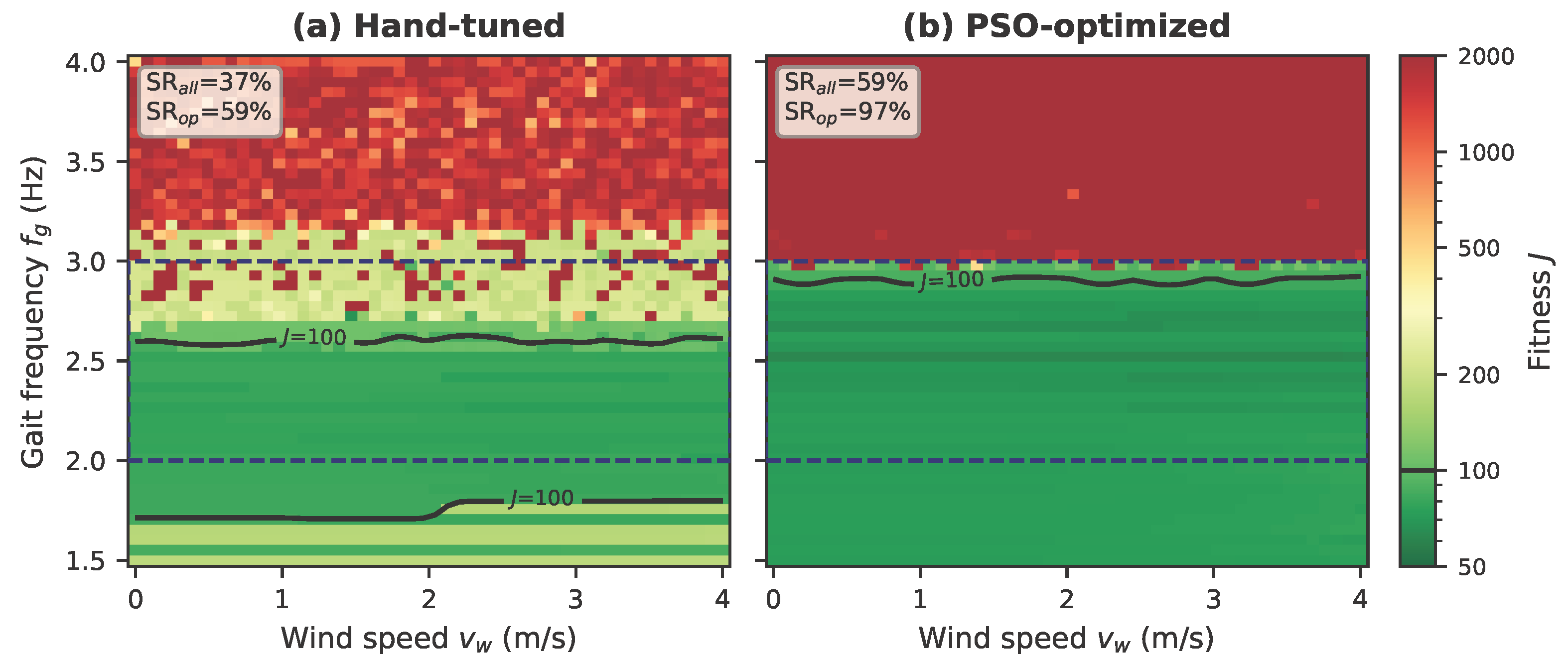
The two dominant environmental factors—gait frequency $f_g$ and wind speed $v_w$—are swept over a $50\times 50$ uniform grid with $f_g\in [1.5,4.0]$ Hz and $v_w\in [0,4.0]$ m/s (fixed wind direction ${\psi }_w=0.5$ rad). The PSO training distribution uses $f_g\in [2.0,3.0]$ Hz and $v_w\in [0,3.0]$ m/s; the cross-validation grid extends to 1.5 Hz, 4.0 Hz, and 4.0 m/s to test out-of-distribution robustness. UAV mass is held at the nominal value $m_0=2.5$ kg to isolate the effects of gait frequency and wind.

The success criterion follows the docking definition in Section 2.5 and is evaluated through the same scalar fitness used during optimisation. A successful run must meet position, attitude, contact-velocity, and bounded-excursion limits. Each of the 2500 grid cells runs one full 20 s docking simulation per parameter configuration, yielding 5000 simulations total (2500 hand-tuned + 2500 PSO-optimised). A simulation is classified as a docking success if the composite fitness satisfies $J_{\mathrm{PSO}}<100$, i.e., the docking penalty (+100 for failure) is not triggered. This binary criterion is more stringent than simply checking the final position, as it also requires bounded attitude excursion, low contact velocity, and sub-50 mm final position error (via (58)).

The validation metrics summarise robustness across the grid. The overall success rate measures global robustness, whereas the operational-band success rate focuses on the gait frequencies expected during normal wheel-legged walking. Two aggregate metrics are reported: the overall success rate (SR), defined as the fraction of all 2500 grid cells achieving $J_{\mathrm{PSO}}<100$, and the operational-band SR restricted to $f_g\in [2.0,3.0]$ Hz (typical quadruped walking cadences).

4.4. Optimisation Results

The optimisation results are reported in three steps: convergence of the swarm, physical interpretation of the optimised parameters, and Monte Carlo generalisation outside the PSO training distribution.

4.4.1. PSO Convergence

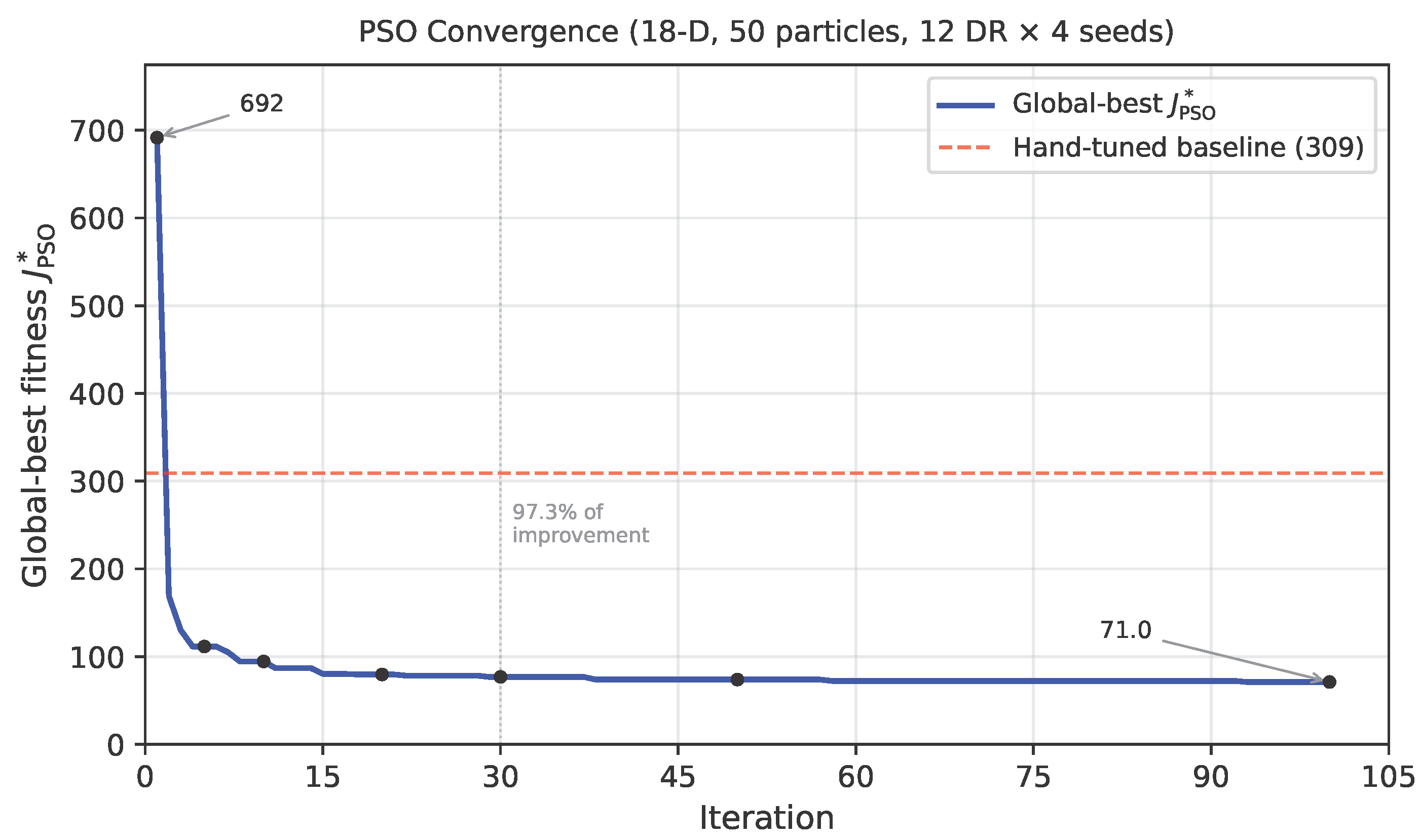
Figure 12 shows the global-best fitness $J_{\mathrm{PSO}}^{\ast }$ versus iteration. The initial swarm-best fitness is $691.58$ (predominantly driven by the docking-failure penalty from randomly initialised particles). Rapid improvement occurs in the first 30 iterations, reducing $J_{\mathrm{PSO}}^{\ast }$ to $76.83$—a 99.1% share of the total $691.58\to 71.02$ improvement. The curve then enters a plateau: iterations 30–100 contribute only incremental refinement ($76.83\to 71.02$), confirming that the 100-iteration budget is sufficient and the swarm has effectively converged. The final improvement occurs at iteration 93 ($72.21\to 71.02$), after which no further progress is observed.

To verify the robustness of the optimised parameters, the final g-best vector is re-evaluated under an independent protocol: 8 random seeds × 12 DR conditions (96 episodes), yielding a mean fitness of $146.05$ compared to $309.07$ for the hand-tuned baseline—a 52.7% improvement. The difference between the g-best fitness (71.02) and the re-evaluation mean (146.05) reflects the broader DR sampling in the independent test (which includes harder conditions near the boundary of the training distribution).

4.4.2. Optimised Parameters

The optimised parameter vector has a clear physical interpretation and reveals three dominant parameter shifts. First, attitude gains are dramatically increased ($k_1^{\mathrm{att}}:7.1\to 29.5$, $+315\%$): the hand-tuned baseline underestimated the gains required for the folded configuration, and since moment arms shrink substantially during folding, the $\alpha$-scheduling (40) amplifies these nominal gains to maintain bandwidth; the PSO raises the baseline so that even the deployed configuration tracks more tightly. Second, observer bandwidths and velocity correction are massively increased ($L_{\mathrm{pos}}:2.9\to 12.6$, ${\mu }_v:6.9\to 17.7$): the hand-tuned observer was overly conservative, and the increased disturbance-channel gain (${\ell }_3:0.21\to 2.27$, $+998\%$) dramatically improves broadband rejection beyond what the internal-model harmonics provide. Third, the internal-model adaptation rate is reduced (${\gamma }_n:104.5\to 14.9$, $-86\%$)—a counter-intuitive shift that compensates for the much higher observer bandwidth: with a faster broadband observer, the IM adaptation can afford to be slower, avoiding interactions between the IM dynamics and the finite-time observer transient; the increased $\sigma$-modification coefficient (${\sigma }_{\mathrm{IM}}:0.19\to 0.29$) reinforces this conservative tuning. The position-loop CFNTSM gains remain largely unchanged ($k_1^{\mathrm{pos}}$: $+12\%$, $k_2^{\mathrm{pos}}$: $-20\%$), suggesting that the original position tracking was adequate and the primary bottleneck was attitude regulation during folding.

Table 5. Hand-tuned vs. PSO-optimised parameter values.

Parameter	Hand-Tuned	PSO-Optimised	Change
$k_1^{\mathrm{pos}}$	12.66	14.13	$+12\%$
$k_2^{\mathrm{pos}}$	5.63	4.51	$-20\%$
${\beta }_{\mathrm{pos}}$	0.102	0.101	$-1\%$
$k_1^{\mathrm{att}}$	7.11	29.54	$+315\%$
$k_2^{\mathrm{att}}$	25.91	33.08	$+28\%$
${\beta }_{\mathrm{att}}$	0.770	1.097	$+42\%$
$p/q$	1.064	1.059	$-0\%$
${\rho }_1$	0.691	0.706	$+2\%$
${\ell }_1$	1.61	1.37	$-15\%$
${\ell }_2$	1.73	3.35	$+94\%$
${\ell }_3$	0.206	2.265	$+998\%$
$L_{\mathrm{pos}}$	2.91	12.57	$+332\%$
$L_{\mathrm{att}}$	9.39	13.92	$+48\%$
${\epsilon }_1$	0.188	0.069	$-63\%$
${\gamma }_n$	104.5	14.93	$-86\%$
${\mu }_v$	6.88	17.67	$+157\%$
${\sigma }_{\mathrm{IM}}$	0.191	0.287	$+50\%$
${\hat{d}}_{max}$	99.4	62.24	$-37\%$

lists the optimised values alongside the hand-tuned initialisations.

4.4.3. Monte Carlo Cross-Validation

Figure 13 and

Table 6. Monte Carlo cross-validation results ($50\times 50$ = 2500 conditions per configuration).

Metric	Hand-Tuned	PSO-Optimised
Overall success rate (%)	37	59
Operational-band SR (%, $f_g\in [2,3]$ Hz)	59	97

summarise the $50\times 50$ cross-validation results. The overall docking success rate increases from 37% to 59%, and within the operational gait-frequency band $f_g\in [2.0,3.0]$ Hz the rate reaches 97%, up from 59%. Figure 13 visualises the per-cell fitness $J_{\mathrm{PSO}}$ on a logarithmic colour scale across the $(f_g,v_w)$ grid; the solid contour marks the $J=100$ success boundary. The hand-tuned configuration (a) achieves low fitness only in a narrow band $f_g\approx 1.8$–$2.6$ Hz, with scattered failures even within this range at higher wind speeds. The PSO-optimised configuration (b) extends the low-fitness region to $f_g\in [1.5,2.9]$ Hz across the full wind range $v_w\in [0,4]$ m/s, with sharply increasing fitness only at $f_g\ge 3.1$ Hz where the gait harmonics approach the Nyquist limit of the 50 Hz control loop.

The residual failures at high $f_g$ are not a parameter-tuning deficiency but rather reflect a fundamental limitation: at $f_g=4$ Hz, the third gait harmonic ($2f_g=8$ Hz) exceeds the observer bandwidth even in enhanced-gain mode, causing the disturbance estimate to lag behind the actual perturbation. These conditions fall outside the target operational envelope and would require architectural changes (e.g., a higher control rate or additional IM harmonics) rather than parameter re-tuning. The PSO-optimised parameters are used in all subsequent simulation experiments (Section 5).

5. Simulation Results

The proposed controller is evaluated through three experiment groups of increasing scope: precision landing and docking (Section 5.2), payload-adaptive takeoff (Section 5.3), and a full end-to-end mission cycle (Section 5.4). All experiments use the PSO-optimised parameters from Section 4 and share the simulation environment described below.

5.1. Simulation Environment

The simulation is implemented in custom Python code (Python 3.8.10; NumPy 1.24.4 for numerical computation and Matplotlib 3.7.5 for plotting) with a 6-DoF rigid-body integrator (RK4, $\mathrm{\Delta }t=1$ ms). The foldable-quadrotor dynamics (8) and (9) with fold-angle-dependent inertia (Table 1) and the walking-robot gait model (21) are evaluated at every time step. The Cheeseman–Bennett ground-effect model (16) is active for $z<4R_p$. Motor dynamics are modelled as first-order with ${\tau }_m=20$ ms. Sensor noise is additive Gaussian: position ${\sigma }_p=0.5$ mm, attitude ${\sigma }_{\eta }={0.1}^{°}$, angular rate ${\sigma }_{\omega }={0.5}^{°}$/s.

The nominal scenario parameters are: dog walking speed $v_d=0.5$ m/s (gait frequency $f_g=2.5$ Hz), lateral wind $v_w=2$ m/s (constant), and initial UAV position $(0,0,2.0)$ m with the dog at the origin heading along the $+x$ axis.

Compared methods. Five configurations are tested in Experiment 1 and four in Experiment 2. All learning-based methods use the same pre-trained FiLM-SAC policy (10 M environment steps with domain randomisation).

Table 7. Compared methods and active components. A check mark indicates that the component is active, whereas—indicates that the component is absent.

ID	Method	CFNTSM	GFA-FEO	FiLM-SAC	$\mathit{\alpha }$-Sched.	Adaptive $\mathit{\lambda }$
M1	Ours (Full)	✓	✓	✓	✓	✓
M2	w/o RL	✓	✓	—	✓	—
M3	w/o GFA	✓	FEO only	✓	—	✓
M4	Fixed-$\lambda$	✓	✓	✓	✓	$\lambda =0.3$
M5	PID	PID	—	—	—	—

summarises the methods and indicates which components are active.

5.2. Experiment 1: Precision Landing and Docking

Experiment 1 isolates the most critical part of the mission: terminal landing and EPM docking on the walking platform. Ablated variants remove FiLM-SAC, GFA-FEO, or adaptive $\lambda$ to quantify the role of each layer against the PID baseline.

Figure 14 first visualises the representative landing geometry before the aggregate metrics are reported. The grey deck marks the $300\times 180$ mm walking-platform landing surface, and the green band denotes the $\pm 10$ mm EPM alignment tolerance. M1 follows a smooth, direct descent with sub-centimetre lateral deviations during the final 0.5 m, whereas M2 (w/o RL) exhibits larger lateral excursions during $M_3$–$M_4$, and M5 (PID) shows sustained oscillations that prevent clean convergence to the docking window.

The UAV starts at ${\mathbf{p}}_0=(0,0,2.0)$ m and must dock on the robot’s back while the robot walks at $v_d=0.5$ m/s. The mission proceeds through the three FSM phases—approach, descent, and docking; arms fold from deployed ($\alpha ={45}^{°}$) to fully stowed ($\alpha =-{76.5}^{°}$) during descent. Each method is evaluated over 100 independent runs at each of three gait frequencies $f_g\in \{2.0,2.5,2.8\}$ Hz, with domain randomisation of wind direction and speed (0–5 m/s), mass ($\pm 10\%$), approach duration (1–3 s), and descent duration (6–10 s). A run is declared successful if and only if condition (22) is satisfied within 20 s.

Table 8. Experiment 1 results ($f_g=2.5$ Hz): precision landing and docking (100 runs per method; mean ± std).

Metric	M1	M2	M3	M4	M5
Pos. RMSEdock (mm) ↓	$\mathbf{4.2}\pm \mathbf{0.7}$	$7.2\pm 0.5$	$5.4\pm 2.0$	$5.6\pm 0.5$	$7.9\pm 1.1$
Att. RMSEdock (°) ↓	$\mathbf{2.0}\pm \mathbf{0.2}$	$2.1\pm 0.2$	$1.9\pm 0.3$	$2.1\pm 0.2$	$2.4\pm 0.1$
Pos. RMSEdesc (mm) ↓	$\mathbf{6.5}\pm \mathbf{0.7}$	$9.3\pm 2.8$	$6.9\pm 0.7$	$8.2\pm 0.7$	$11.9\pm 3.1$
Contact vel. (m/s) ↓	$0.070\pm 0.027$	$0.067\pm 0.028$	$0.061\pm 0.025$	$0.070\pm 0.029$	$0.016\pm 0.010$
Success rate (%) ↑	$\mathbf{100}$	99	92	100	94
Peak att. excursion (°) ↓	$5.0\pm 0.7$	$4.8\pm 1.2$	$4.8\pm 0.7$	$4.7\pm 0.6$	$3.3\pm 0.5$

Note: Bold indicates the best value for each metric where applicable.

reports the nominal condition $f_g=2.5$ Hz; cross-frequency results are discussed below.

5.2.1. Docking Quantitative Results

Table 8 compares docking precision, attitude matching, contact speed, and success rate across the full controller and four ablated baselines. Each value is computed from 100 randomised runs with wind, mass, timing, and gait perturbations.

Table 8 shows that M1 (Ours Full) achieves the best docking position RMSE ($4.2$ mm) and maintains a $100\%$ success rate across all three tested gait frequencies. Statistical significance is assessed via Welch’s t-test on the per seed docking position RMSE. The key observations are:

(i) Necessity of the residual RL (M1 vs. M2). Removing FiLM-SAC increases the docking position RMSE by 71% (from 4.2 to 7.2 mm, $p=6.2\times {10}^{-85}$) and the descent-phase RMSE by 43% (from 6.5 to 9.3 mm). At $f_g=2.5$ Hz M2’s success rate is 99%; at $f_g=2.8$ Hz, it drops further to 94%, whereas M1 remains at 100% across all frequencies. The performance gap is most pronounced during descent, where the RL residual compensates for the unmodelled aerodynamic coupling between folding arms and the time-varying allocation matrix—nonlinearities outside the GFA-FEO’s disturbance class.

(ii) Necessity of the GFA framework (M1 vs. M3). Replacing GFA-FEO—which combines gait-frequency internal-model harmonics at $f_g/2$, $f_g$, and $2f_g$ with $\alpha$-scheduled gains—with a standard FEO increases the docking RMSE by 29% (from 4.2 to 5.4 mm, $p=7.0\times {10}^{-8}$) and reduces the success rate from 100% to 92%. The standard FEO cannot fully cancel the periodic gait disturbance nor compensate for the fold-angle-dependent control effectiveness, leading to a substantially higher variance ($\pm 2.0$ mm vs. $\pm 0.7$ mm) that reflects inconsistent performance across domain-randomised conditions. At $f_g=2.8$ Hz, the gap persists (4.5 vs. 5.0 mm, SR $100\%\to 95\%$), confirming the benefit at higher gait frequencies where the periodic disturbance is more aggressive.

(iii) Benefit of adaptive $\lambda \left(t\right)$ (M1 vs. M4). Fixing $\lambda =0.3$ (the time average of the adaptive gate) increases the docking RMSE by 33% (from 4.2 to 5.6 mm, $p=5.1\times {10}^{-39}$) and the descent-phase RMSE by 26% (from 6.5 to 8.2 mm). Both methods maintain 100% success at $f_g\le 2.5$ Hz (M4 drops to 99% at $f_g=2.8$ Hz); the primary difference lies in precision. The adaptive law concentrates RL authority during descent and docking, where it matters most, while attenuating RL influence during the approach phase, where the model-based controller already suffices.

(iv) PID baseline (M5). Despite PSO-optimised gains, the PID controller achieves a docking RMSE of 7.9 mm—88% worse than M1 ($p=2.9\times {10}^{-65}$)—and a descent-phase RMSE of 11.9 mm (83% worse). Its success rate drops to 90% at $f_g=2.0$ Hz and 87% at $f_g=2.8$ Hz. Without observer-based disturbance compensation, the gait-induced oscillation propagates directly into the position loop, and the absence of gain scheduling produces fixed control authority that cannot adapt to the varying allocation matrix during arm folding. Notably, PID exhibits the lowest peak attitude excursion (${3.3}^{°}$ vs. M1’s ${5.0}^{°}$) and lowest contact velocity ($0.016$ m/s vs. $0.070$ m/s), reflecting its conservative gains; however, this conservatism comes at the cost of substantially worse tracking precision.

5.2.2. Time-Series Analysis

Figure 15 presents the time histories of key signals for M1 during a representative run. The FSM phases $M_1$–$M_6$ are indicated by background shading. The GFA-FEO disturbance estimate ${\hat{d}}_z$ tracks the phase and frequency of the true gait-induced acceleration but attenuates the peak amplitude by approximately 50%. This is an intentional consequence of the leakage term ${\sigma }_{\mathrm{IM}}$ in the internal-model adaptation law (32): setting ${\sigma }_{\mathrm{IM}}>0$ prevents the Fourier coefficients from diverging when the actual gait frequency deviates from the nominal value, at the cost of a steady-state amplitude bias.

Panel (a) confirms that the vertical error remains inside the $\pm 10$ mm docking tolerance after capture, while panel (b) compares the UAV roll angle with the landing-surface roll and zooms into the descent interval. In panel (c), the GFA-FEO estimate ${\hat{d}}_z$ is overlaid with the scaled gait heave acceleration; the Pearson correlation $r=0.86$ and amplitude ratio 0.45 show that the observer captures the dominant phase while intentionally attenuating the amplitude. The uncompensated residual—visible as the gap between the grey and red envelopes—is precisely the broadband disturbance that the RL residual $\mathit{\delta }\mathit{u}$ corrects, explaining why removing FiLM-SAC (M2) degrades tracking by 71%. Panel (d) shows that $\lambda \left(t\right)$ peaks at ≈0.4 during $M_3$, where fold-through causes the strongest gait coupling, and falls to near zero during $M_5$ after locking.

Off-diagonal coupling verification. As noted in Section 3.5, the off-diagonal terms of ${\mathbf{g}}_{\eta }\left(\alpha \right)$ are treated as part of the lumped disturbance. At the most extreme fold angle $\alpha =-{76.5}^{°}$, the maximum off-diagonal-to-diagonal ratio is ${max}_{i\ne j}|g_{\eta ,ij}|/{min}_i\left|g_{\eta ,ii}\right|=0.18$, confirming the approximation is valid (the GFA-FEO estimates this coupling as part of ${\mathbf{d}}_{\eta }$).

5.3. Experiment 2: Payload-Adaptive Takeoff

Experiment 2 evaluates the opposite transition: after docking, the UAV must take off while carrying the robot as payload. This test focuses on whether the hot-switch protocol correctly updates the observer and plant model after the sudden mass and inertia change.

Starting from the fully stowed and locked state ($M_6$: $\alpha =-{76.5}^{°}$, coupled mass $m_c=5.00$ kg), the UAV receives a takeoff command and must climb to $z=3.0$ m while unfolding arms ($\alpha :-{76.5}^{°}\to {45}^{°}$) and stabilising the coupled body. A lateral wind gust of 1–5 m/s is applied at a randomised time $t_{\mathrm{gust}}\in [1,3]$ s. Each method is evaluated over 100 independent runs with randomised wind direction and speed, ramp duration (2–4 s), unfold duration (3–5 s), mass perturbation ($\pm 10\%$), and sensor noise.

Four methods are compared (Table 7): M1 (Ours Full with hot-switch), M2 (w/o RL), a variant M1′ that omits the hot-switch protocol (the observer retains pre-locking parameters), and M5 (PID with hot-switch).

Takeoff Quantitative Results

Table 9. Experiment 2 results: payload-adaptive takeoff (100 runs per method; mean ± std).

Metric	M1	M2	M1′ (No HS)	M5
Altitude overshoot (cm) ↓	$\mathbf{0.4}\pm \mathbf{0.2}$	$0.2\pm 0.1$	$0.3\pm 0.5$	$5.1\pm 1.8$
Settling time to ±5 cm (s) ↓	$2.8\pm 0.5$	$\mathbf{2.8}\pm \mathbf{0.5}$	$2.8\pm 0.5$	$2.9\pm 0.3$
Peak roll excursion (°) ↓	$\mathbf{3.4}\pm \mathbf{0.4}$	$2.9\pm 0.4$	$5.7\pm 1.6$	$7.7\pm 2.2$
Pos. RMSE $t\in [0,5]$ s (mm) ↓	$16.2\pm 1.8$	$\mathbf{13.9}\pm \mathbf{2.1}$	$44.2\pm 24.8$	$27.9\pm 6.4$

Note: Bold indicates the best value for each metric where applicable.

focuses on the transient response after the EPM lock and payload takeoff command. In addition to altitude tracking, it reports peak roll excursion and early-window position RMSE, both of which are sensitive to the observer and plant-model reset.

The main observations are as follows.

(i) FEO hot-switch is critical (M1 vs. M1′). Without hot-switching, the observer retains the pre-locking mass $m_u=2.50$ kg in its internal model. The resulting plant-model mismatch ($m_c/m_u=2.0$) causes the FEO to grossly overestimate the control effectiveness, leading to a position RMSE that almost triples (from 16.2 to 44.2 mm, $p=2.3\times {10}^{-19}$) and peak roll excursions that increase by 68% (from ${3.4}^{°}$ to ${5.7}^{°}$). Figure 16c shows the initial 85 mm position error spike caused by the mass mismatch, followed by persistent oscillations of 15–30 mm.

(ii) CFNTSM + FEO vs. PID (M1 vs. M5). The PID controller, despite PSO-optimised gains, exhibits 12× higher altitude overshoot ($5.1$ vs. $0.4$ cm) and 72% worse position RMSE ($27.9$ vs. $16.2$ mm, $p=1.9\times {10}^{-34}$). Panel (c) shows that M5 suffers large error transients after the wind gust, reflecting the lack of model-based disturbance compensation.

(iii) Role of RL during takeoff (M1 vs. M2). M2 (model-based controller only, $\mathit{\delta }\mathit{u}=\mathbf{0}$) achieves slightly lower RMSE than M1 (13.9 vs. 16.2 mm). This result is expected: the FiLM-SAC policy was trained exclusively for the landing phase (Exp. 1), and its residual actions—calibrated for descent/docking dynamics—are not optimised for the fundamentally different takeoff trajectory. The 17% overhead confirms that the residual RL is benign (not destabilising) even when operating outside its training distribution, while the model-based controller alone is sufficient for the less demanding takeoff task.

Figure 16 visualises the corresponding trajectory and disturbance-estimation behaviour.

5.4. Experiment 3: Full Mission Cycle

Experiment 3 combines the preceding phases into a continuous mission cycle. The trajectory passes through approach, folding, docking, payload takeoff, cruise, and final delivery to test error boundedness across phase transitions.

5.4.1. Scenario

The full mission unfolds over 40 s and traverses six phases. The primary evaluation uses M1 (Ours Full); a PSO-tuned PID baseline (M5) is overlaid in the timeline figure for visual comparison. Phase I (0–5 s) is a cruise approach at $z=2.0$ m with arms deployed ($\alpha ={45}^{°}$). In Phase II (5–8 s) a cosine-ramp descent brings the UAV from $z=2.0$ m to $z_{\mathrm{dog}}=0.35$ m while the arms fold proportionally (${45}^{°}\to -76.5$). Phase III (8–11 s) is the docking hold: EPM lock triggers when $\parallel e_p\parallel <15$ mm, $\parallel e_{\eta }\parallel <5^{°}$, and $|\dot{z}-{\dot{z}}_{\mathrm{gait}}|<0.10$ m/s are sustained for 0.3 s: the hot-switch protocol (Section 3.9) fires. Phase IV (11–16 s) is takeoff with the coupled body via a cosine ramp to $z_{\mathrm{del}}=3.0$ m while the arms unfold. Phases V–VI (16–40 s) comprise the cruise to the delivery altitude and station-keeping. Domain randomisation matches Experiments 1–2: $m\sim \mathcal{U}(0.9,1.1)m_{\mathrm{nom}}$, $f_g\sim \mathcal{U}(2.0,2.8)$ Hz, wind speed $\sim \mathcal{U}(0,5)$ m/s with random direction. The RL residual is gated: active in Phases II–IV (descent, dock, and takeoff) and disabled in Phases I, V, VI (cruise and station-keep). Each of 100 seeds produces one complete 40 s trajectory.

5.4.2. Mission Timeline

Figure 17 shows a representative mission. The system achieves a 100% docking success rate and 100% mission completion rate across all 100 runs. Docking lock-on occurs at $t=8.75\pm 0.20$ s (i.e., $0.75$ s into Phase III), confirming rapid convergence to the surface.

Panel (a) shows altitude tracking: the actual trajectory follows the commanded cosine-ramp descent to the dog surface, docking hold, and ascent to the delivery altitude. Panel (b) reports the fold-angle trajectory, where $\alpha \left(t\right)$ completes the full cycle ${45}^{°}\to -{76.5}^{°}\to {45}^{°}$. Panel (c) compares the position-error norm of M1 with the PID baseline; M1 peaks during descent fold-through and then settles below 10 mm in cruise, whereas PID remains substantially less accurate throughout the mission. Panel (d) overlays the FEO vertical disturbance estimate with the scaled gait heave acceleration, showing that the observer tracks the periodic gait component across the phase sequence, including after the mass-doubling transition; the PID baseline has no corresponding disturbance observer.

Table 10. Experiment 3: per-phase position RMSE for M1 (Ours Full) and M5 (PID), each over 100 runs (mean ± std). Attitude RMSE (M1) is reported for the phases where gait-coupled attitude tracking is most critical.

Phase	M1 Pos. RMSE (mm)	M5 Pos. RMSE (mm)	M1 Att. RMSE (°)	Key Challenge
I Approach	$6.07\pm 0.54$	$8.18\pm 1.05$	—	Gait tracking
II Descend	$16.90\pm 2.55$	$37.73\pm 12.49$	$2.51\pm 0.68$	$\alpha$ fold-through
III Dock	$5.06\pm 1.00$	$17.27\pm 2.99$	$2.09\pm 0.08$	Surface hold
IV Takeoff	$11.78\pm 0.32$	$15.26\pm 0.77$	—	Mass doubling
V Cruise	$4.61\pm 0.36$	$7.64\pm 0.51$	—	Coupled cruise
VI Station	$4.22\pm 0.17$	$7.52\pm 0.53$	—	Long-term hold
Peak error (mission-wide)		M1: $27.43\pm 3.63$ mm/M5: $62.51\pm 20.34$ mm
Docking time		M1: $8.75\pm 0.20$ s/M5: $8.87\pm 0.20$ s

reports position and attitude RMSE by phase for both M1 (Ours Full) and M5 (PID), each evaluated over 100 random seeds. These phase-wise metrics provide the numerical basis for interpreting where the full mission is most demanding and where the proposed controller gains the largest advantage over PID.

For M1, the most demanding interval is Phase II (descent), with position RMSE $16.90\pm 2.55$ mm and attitude RMSE $2.51\pm {0.68}^{°}$, driven by the simultaneous altitude ramp and arm folding through the minimum-${\sigma }_2$ region. This phase combines the least favourable actuator geometry with the strongest gait-induced deck motion, so it is the point at which the gain scheduler and disturbance observer are most heavily exercised. Phase IV (takeoff) produces the second-largest transient ($11.78\pm 0.32$ mm) because the EPM-locked system undergoes a sudden mass-doubling step and FEO re-initialisation before the observer states settle to the coupled-body dynamics. After the transition settles, Phase V (cruise) and Phase VI (station-keep) exhibit the tightest tracking: $4.61\pm 0.36$ mm and $4.22\pm 0.17$ mm, respectively, confirming that the observer and gain scheduler fully adapt to the coupled-body dynamics.

The peak instantaneous position error across the entire mission is $27.43\pm 3.63$ mm, occurring during the descent-to-dock transition, and it remains below the tolerance margin required for magnetic capture.

By contrast, the PID baseline (M5) exhibits a mission-wide peak error of $62.51\pm 20.34$ mm—$2.3\times$ larger than M1—with the worst degradation in Phase II ($37.73\pm 12.49$ mm vs. $16.90$ mm for M1) and Phase III ($17.27\pm 2.99$ mm vs. $5.06$ mm). The largest gap, therefore, occurs exactly where the system requires fold-aware allocation, gait-frequency disturbance rejection, and residual correction simultaneously. These results confirm that the CFNTSM + GFA-FEO architecture with RL residual provides substantially better disturbance rejection than a tuned PID controller across the full mission (Figure 17c,d).

5.4.3. 6-DoF Error Panorama

Figure 18 decomposes the tracking error into six channels over the full 40 s. The most informative observations are as follows. During descent fold-through ($t\approx 5$–8 s), $e_z$ peaks at ∼20 mm as $\alpha$ traverses the minimum-${\sigma }_2$ region; the adaptive gain scheduler (40) maintains control authority. At the mass transition ($t\approx 8$ s), the FEO reset produces a brief $e_x$ spike (∼10 mm) that decays within $0.5$ s.

During post-coupling takeoff ($t\approx 11$ s), $e_z$ shows a smooth ∼15 mm undershoot during the cosine-ramp ascent with doubled mass, fully absorbed by the CFNTSM. Yaw coupling remains small ($e_{\psi }<1^{°}$ during mass transitions, <0.1° in cruise), confirming that four-rotor yaw authority is preserved even at ${\alpha }_{\mathrm{fold}}$. In all critical intervals, the errors remain well within the docking tolerance or recover within 0.5 s, confirming that the gain scheduling, hot-switch, and RL residual mechanisms work in concert to maintain tracking across the full flight envelope.

The temporal error distribution also explains why the full-stack controller outperforms the PID baseline in the mission-level statistics. The largest excursions coincide with known physical events—fold-through, magnetic locking, payload coupling, and takeoff mass doubling—rather than with slow drift or accumulated observer bias. This indicates that the remaining error is dominated by short, bounded transients at mode transitions, while the controller recovers to millimetre-level tracking during the quasi-steady cruise and station-keeping phases.

5.5. Summary of Results

Table 11. Summary of key results across experiments.

Finding	Exp.	Compared	Result
RL residual necessity	1	M1 vs. M2	Dock RMSE $-42$% ($4.2$ vs. $7.2$ mm, $p<{10}^{-84}$)
GFA internal model	1	M1 vs. M3	Dock RMSE $-22$% ($4.2$ vs. $5.4$ mm), SR $+8$ pp
Adaptive $\lambda \left(t\right)$	1	M1 vs. M4	Dock RMSE $-25$% ($4.2$ vs. $5.6$ mm, $p<{10}^{-38}$)
FEO hot-switch	2	M1 vs. M1′	Pos. RMSE $-63$% ($16.2$ vs. $44.2$ mm, $p<{10}^{-18}$)
CFNTSM + FEO vs. PID	2	M1 vs. M5	Pos. RMSE $-42$% ($16.2$ vs. $27.9$ mm, $p<{10}^{-33}$)
Full-cycle feasibility	3	M1 vs. M5	100% SR; peak err. M1 $27.4$ vs. M5 $62.5$ mm

consolidates the key findings across all three experiments and links each result to the control module that it isolates. Experiment 1 explains the landing-side accuracy gains by separating the contributions of the RL residual, gait-frequency-aware observer, and adaptive trust weight. Experiment 2 tests the payload transition and shows that the hot-switch protocol is needed when the coupled mass and inertia change abruptly. Experiment 3 then verifies that these improvements remain compatible over the full docking-to-delivery mission rather than only in isolated phases.

Taken together, the results show that no single layer accounts for the reported performance. The model-based CFNTSM + GFA-FEO backbone supplies bounded tracking and periodic disturbance rejection, the fold-aware scheduling preserves authority through changing geometry, and the FiLM-SAC residual improves precision in the nonlinear descent and docking regime. The table, therefore, serves as a compact cross-check between the ablation evidence, the payload-takeoff validation, and the complete-mission benchmark.

6. Discussion

The three experiment groups indicate that reliable docking on a walking platform depends on the coordinated action of all control layers rather than on any single module. The model-based CFNTSM + GFA-FEO backbone rejects the dominant gait-periodic disturbance and adapts the control gains to the fold-dependent allocation matrix $\mathbf{B}\left(\alpha \right)$. The FiLM-SAC residual then compensates for unmodelled aerodynamic coupling between the folding arms and rotor wake, which lies outside the disturbance class represented by the linear internal model, while the adaptive trust weight $\lambda \left(t\right)$ concentrates learned authority during descent and docking. The ablation results in Table 11 therefore support the intended division of labour: observer-based periodic rejection, fold-aware finite-time control, and bounded learned residual compensation each provide a statistically significant reduction in tracking error.

The hot-switch protocol is particularly important during the transition from docking to payload-carrying takeoff. Without updating the plant model at magnetic locking (M1′), the twofold mass mismatch produces a 173% increase in takeoff RMSE (Table 11). Under domain randomisation, the observer reset, boosted bandwidth, bounded residual authority, and fallback climb/hold condition collectively prevent the blind window from becoming an open-loop interval. The residual policy was trained only for landing and still introduces only a modest 17% overhead in the takeoff comparison, suggesting that the learned component remains well bounded outside its primary training distribution; nevertheless, including takeoff transients in future residual-policy training should further reduce this margin.

The full-mission experiment demonstrates completion of a 40 s, six-phase docking-to-delivery cycle in simulation. Across 100 randomised seeds, both the docking and mission success rates remain at 100%, indicating that the FSM transitions, gain scheduler, FEO re-initialisation, and RL gating operate coherently over the complete sequence. The largest position error ($27.4\pm 3.6$ mm) occurs during descent fold-through, where ${\sigma }_2\left(\mathbf{B}\right)$ reaches its minimum and the vehicle is in its most mechanically constrained configuration. Even in this interval, the transient remains within the EPM capture tolerance and decays rapidly after the mode transition.

Several limitations should be noted. Although a full-scale hardware prototype has been assembled (Section 2.6), the present results are derived from numerical simulation with domain randomisation and synthetic sensor noise. Flight experiments on the physical Jetson Orin Nano/PX4 platform, therefore, represent the immediate next step. On the perception side, the study assumes sub-centimetre relative-pose accuracy, whereas outdoor deployment will require real-time fusion of RealSense D415 visual/depth updates, Unitree L2 LiDAR registration, and inertial measurements in the onboard estimator. On the mechanical side, the crank-rocker mechanism satisfies the Grashof condition with a geometric margin of only 0.3 mm. Hardware validation must therefore verify repeatability under tolerance stack-up, servo heating, gear backlash, and repeated high-frequency folding. The design mitigates these risks through joint clearance, mechanical end-stops, a slew-limited 0.6 s fold command and current/fold-angle consistency checks for jam detection, but these provisions still require bench endurance testing before aggressive in-flight morphing is attempted. Finally, the FiLM-SAC policy was trained at a single gait frequency and evaluated over $f_g\in [2.0,2.8]$ Hz; extending validation to broader gait speeds and different robot morphologies, and evaluating multi-joint folding architectures that preserve greater control authority at extreme fold angles constitute important directions for future investigation.

7. Conclusions

This work presents a hierarchical control framework designed for autonomous docking of a foldable quadrotor on a trotting wheel-legged robot, followed by payload-adaptive takeoff. The framework integrates an $\alpha$-scheduled CFNTSM controller, a gait-frequency-aware finite-time extended observer (GFA-FEO), and a FiLM-SAC residual RL policy with an adaptive trust weight $\lambda \left(t\right)$.

The simulation results support three main conclusions. First, the fold-aware CFNTSM + GFA-FEO backbone maintains the vehicle inside the EPM capture window despite gait-induced surface motion and fold-angle authority loss, while the FiLM-SAC residual further reduces docking RMSE from $7.2\pm 0.5$ mm to $4.2\pm 0.7$ mm at $f_g=2.5$ Hz. Second, adaptive trust weighting improves precision relative to a fixed residual weight, reducing docking RMSE by 25%. Third, after EPM locking, the FEO hot-switch protocol is necessary for payload-adaptive takeoff: it reduces the early takeoff RMSE by 63% after the coupled mass approximately doubles. In the complete 40 s simulated mission, the full system achieves 100% success over 100 randomised seeds, with the largest transient position error ($27.4\pm 3.6$ mm) occurring during the mechanically constrained descent fold-through phase.

These conclusions are supported within the simulated and domain-randomised operating envelope considered in this study. Because hardware flight tests have not yet been conducted, these results should be regarded as simulation-level evidence for the proposed mechanism–control concept rather than final field-deployment validation. A hardware prototype has been assembled (Section 2.6); future efforts will target sim-to-real transfer validation, onboard visual-inertial state estimation, and multi-phase reinforcement-learning policy refinement.

References

1. Pretto, A.; Aravecchia, S.; Burgard, W.; Chebrolu, N.; Dornhege, C.; Falck, T.; Fleckenstein, F.; Fontenla, A.; Imperoli, M.; Khanna, R.; et al. Building an Aerial-Ground Robotics System for Precision Farming: An Adaptable Solution. IEEE Robot. Autom. Mag. 2021, 28, 29–49. [Google Scholar] [CrossRef]
2. Zhou, Y.; Quang, L.; Nieto-Granda, C.; Loianno, G. CoPeD—Advancing Multi-Robot Collaborative Perception: A Comprehensive Dataset in Real-World Environments. IEEE Robot. Autom. Lett. 2024, 9, 6416–6423. [Google Scholar] [CrossRef]
3. Wang, J.; Guan, X.; Sun, Z.; Shen, T.; Huang, D.; Liu, F.; Cui, H. OMEGA: Efficient Occlusion-Aware Navigation for Air-Ground Robots in Dynamic Environments via State Space Model. arXiv 2024, arXiv:2408.10618. [Google Scholar] [CrossRef]
4. Xu, H.; Wang, C.; Bo, Y.; Jiang, C.; Liu, Y.; Yang, S.; Lai, W. An Aerial and Ground Multi-Agent Cooperative Location Framework in GNSS-Challenged Environments. Remote Sens. 2022, 14, 5055. [Google Scholar] [CrossRef]
5. Lu, W.; Bin, D.; Ma, L.; Ma, M.; Ma, Z.; Chen, X.; Wang, L.; Feng, Y.; Jiang, Z.; Shi, Y.; et al. Semi-Distributed Cross-Modal Air-Ground Relative Localization. arXiv 2025, arXiv:2511.06749. [Google Scholar]
6. Shi, Y.; Hua, Y.; Yu, J.; Dong, X.; Lü, J.; Ren, Z. Cooperative Fault-Tolerant Formation Tracking Control for Heterogeneous Air–Ground Systems Using a Learning-Based Method. IEEE Trans. Aerosp. Electron. Syst. 2024, 60, 1742–1755. [Google Scholar] [CrossRef]
7. Yang, J.-X.; Xu, Y.; Wu, Z.-G.; Li, Y. Distributed Estimation and Data-Driven Formation Control of Air–Ground Systems via Efficient Reinforcement Learning. IEEE Trans. Aerosp. Electron. Syst. 2025, 61, 16622–16633. [Google Scholar] [CrossRef]
8. Li, Z.; Mao, R.; Chen, N.; Xu, C.; Gao, F.; Cao, Y. ColAG: A Collaborative Air–Ground Framework for Perception-Limited UGVs’ Navigation. In Proceedings of the 2024 IEEE International Conference on Robotics and Automation (ICRA), Yokohama, Japan, 13–17 May 2024. [Google Scholar]
9. Baca, T.; Hert, D.; Loianno, G.; Saska, M.; Kumar, V. Model Predictive Trajectory Tracking and Collision Avoidance for Reliable Outdoor Deployment of Unmanned Aerial Vehicles. In Proceedings of the 2018 IEEE/RSJ International Conference on Intelligent Robots and Systems (IROS), Madrid, Spain, 1–5 October 2018; pp. 6753–6760. [Google Scholar]
10. Keipour, A.; Pereira, G.A.S.; Bonatti, R.; Garg, R.; Rastogi, P.; Dubey, G.; Scherer, S. Visual Servoing Approach to Autonomous UAV Landing on a Moving Vehicle. Sensors 2022, 22, 6549. [Google Scholar] [CrossRef]
11. Chang, C.-W.; Lo, L.-Y.; Cheung, H.C.; Feng, Y.; Yang, A.-S.; Wen, C.-Y.; Zhou, W. Proactive Guidance for Accurate UAV Landing on a Dynamic Platform: A Visual–Inertial Approach. Sensors 2022, 22, 404. [Google Scholar] [CrossRef]
12. Huang, Y.; Zhu, M.; Zheng, Z.; Low, K.H. Linear Velocity-Free Visual Servoing Control for Unmanned Helicopter Landing on a Ship With Visibility Constraint. IEEE Trans. Syst. Man Cybern. Syst. 2021, 52, 2979–2993. [Google Scholar] [CrossRef]
13. Ollero, A.; Tognon, M.; Suarez, A.; Lee, D.; Franchi, A. Past, Present, and Future of Aerial Robotic Manipulators. IEEE Trans. Robot. 2022, 38, 626–645. [Google Scholar] [CrossRef]
14. Meng, J.; Buzzatto, J.; Liu, Y.; Liarokapis, M. On Aerial Robots With Grasping and Perching Capabilities: A Comprehensive Review. Front. Robot. AI 2022, 8, 739173. [Google Scholar] [CrossRef]
15. Zheng, P.; Xiao, F.; Nguyen, P.H.; Farinha, A.; Kovac, M. Metamorphic Aerial Robot Capable of Mid-Air Shape Morphing for Rapid Perching. Sci. Rep. 2023, 13, 1297. [Google Scholar] [CrossRef]
16. Wüest, V.; Jeger, S.; Feroskhan, M.; Ajanic, E.; Bergonti, F.; Floreano, D. Agile Perching Maneuvers in Birds and Morphing-Wing Drones. Nat. Commun. 2024, 15, 8330. [Google Scholar] [CrossRef]
17. Li, C.-X.; Wu, H.-N.; Yang, T. Coordinated Control of Flight and Morphing for Morphing Quadrotor via Reinforcement Learning. IEEE Trans. Aerosp. Electron. Syst. 2025, 61, 12755–12766. [Google Scholar] [CrossRef]
18. Idrissi, M.; Salami, M.; Annaz, F. A Review of Quadrotor Unmanned Aerial Vehicles: Applications, Architectural Design and Control Algorithms. J. Intell. Robot. Syst. 2022, 104, 22. [Google Scholar] [CrossRef]
19. Singh, K.; Mehndiratta, M.; Feroskhan, M. QuadPlus: Design, Modeling, and Receding Horizon-Based Control of a Hyperdynamic Quadrotor. IEEE Trans. Aerosp. Electron. Syst. 2021, 58, 1766–1779. [Google Scholar] [CrossRef]
20. Lou, H.; Wu, Q.; Wang, H.; Li, M.; Liu, H.; Sun, N. Structure, Modeling, and Control of Morphing Quadrotors: A Review. Int. J. Precis. Eng. Manuf. 2026, 27, 825–842. [Google Scholar] [CrossRef]
21. Falanga, D.; Kleber, K.; Mintchev, S.; Floreano, D.; Scaramuzza, D. The Foldable Drone: A Morphing Quadrotor that can Squeeze and Fly. IEEE Robot. Autom. Lett. 2019, 4, 209–216. [Google Scholar] [CrossRef]
22. Tuna, T.; Ovur, S.E.; Gokbel, E.; Kumbasar, T. Design and Development of FOLLY: A Self-Foldable and Self-Deployable Quadcopter. Aerosp. Sci. Technol. 2020, 100, 105807. [Google Scholar] [CrossRef]
23. Yang, T.; Wu, H.-N.; Wang, J.-W. cc-DRL: A Convex Combined Deep Reinforcement Learning Flight Control Design for a Morphing Quadrotor. arXiv 2024, arXiv:2408.13054. [Google Scholar] [CrossRef]
24. Hu, D.; Pei, Z.; Shi, J.; Tang, Z. Design, Modeling and Control of a Novel Morphing Quadrotor. IEEE Robot. Autom. Lett. 2021, 6, 8013–8020. [Google Scholar] [CrossRef]
25. Cao, C.; Li, F.; Ding, R.; Huang, T.; Yang, C.; Gui, W. Intelligent Attitude Control for Morphing Flight Vehicle: A Deep Reinforcement Learning Approach. IEEE Trans. Veh. Technol. 2025, 74, 8851–8865. [Google Scholar] [CrossRef]
26. Bauersfeld, L.; Kaufmann, E.; Scaramuzza, D. User-Conditioned Neural Control Policies for Mobile Robotics. In Proceedings of the 2023 IEEE International Conference on Robotics and Automation (ICRA), London, UK, 29 May–2 June 2023; pp. 1342–1348. [Google Scholar]
27. Zhang, R.; Zhang, D.; Mueller, M.W. ProxFly: Robust Control for Close Proximity Quadcopter Flight via Residual Reinforcement Learning. In Proceedings of the 2025 IEEE International Conference on Robotics and Automation (ICRA), Atlanta, GA, USA, 19–23 May 2025. [Google Scholar]
28. Ullah, M.; Gao, H.; Nasir, A.; Wang, Y.; Wang, C. Adaptive-Neural Finite-Time Sliding Mode Control for Quadrotor Helicopter Attitude Stabilization in Complex Environments. IEEE Trans. Aerosp. Electron. Syst. 2025, 61, 1175–1185. [Google Scholar] [CrossRef]
29. Wang, S.; Hao, W.; Ma, W.; Mei, T. Reinforcement Learning Based Optimized Sliding Mode Attitude Control Strategy for Quadrotor Against Unknown Time-Varying Disturbances. Eng. Res. Express 2026, in press. [Google Scholar] [CrossRef]
30. Mahmood, A.A.; García, F.; Al-Kaff, A. A Novel Design of a Sliding Mode Controller Based on Modified ERL for Enhanced Quadcopter Trajectory Tracking. Drones 2025, 9, 737. [Google Scholar] [CrossRef]
31. Foehn, P.; Kaufmann, E.; Romero, A.; Penicka, R.; Sun, S.; Bauersfeld, L.; Laengle, T.; Cioffi, G.; Song, Y.; Loquercio, A.; et al. Agilicious: Open-Source and Open-Hardware Agile Quadrotor for Vision-Based Flight. Sci. Robot. 2022, 7, eabl6259. [Google Scholar] [CrossRef]
32. Kaufmann, E.; Bauersfeld, L.; Loquercio, A.; Müller, M.; Koltun, V.; Scaramuzza, D. Champion-Level Drone Racing Using Deep Reinforcement Learning. Nature 2023, 620, 982–987. [Google Scholar] [CrossRef]
33. Dimmig, C.A.; Silano, G.; McGuire, K.; Gabellieri, C.; Hönig, W.; Moore, J.; Kobilarov, M. Survey of Simulators for Aerial Robots: An Overview and In-Depth Systematic Comparisons. IEEE Robot. Autom. Mag. 2024, 32, 153–166. [Google Scholar] [CrossRef]
34. Staessens, T.; Lefebvre, T.; Crevecoeur, G. Adaptive Control of a Mechatronic System Using Constrained Residual Reinforcement Learning. IEEE Trans. Ind. Electron. 2022, 69, 10447–10456. [Google Scholar] [CrossRef]
35. Ishihara, Y.; Hazama, Y.; Suzuki, K.; Yokono, J.J.; Sabe, K.; Kawamoto, K. Improving Wind Resistance Performance of Cascaded PID Controlled Quadcopters Using Residual Reinforcement Learning. arXiv 2023, arXiv:2308.01648. [Google Scholar] [CrossRef]
36. Wen, S.; Shu, Y.; Rad, A.; Wen, Z.; Guo, Z.; Gong, S. A Deep Residual Reinforcement Learning Algorithm Based on Soft Actor-Critic for Autonomous Navigation. Expert Syst. Appl. 2025, 259, 125238. [Google Scholar] [CrossRef]
37. Hua, H.; Fang, Y. A Novel Reinforcement Learning-Based Robust Control Strategy for a Quadrotor. IEEE Trans. Ind. Electron. 2023, 70, 2812–2821. [Google Scholar] [CrossRef]
38. Yu, C.; Rosendo, A. Multi-Modal Legged Locomotion Framework with Automated Residual Reinforcement Learning. IEEE Robot. Autom. Lett. 2022, 7, 10312–10319. [Google Scholar] [CrossRef]
39. McN. Alexander, R. Mechanics of bipedalism. In Scale Effects in Animal Locomotion; Academic Press: London, UK, 1977; pp. 93–110. [Google Scholar]
40. Qin, T.; Pan, J.; Cao, S.; Shen, S. A General Optimization-Based Framework for Local Odometry Estimation With Multiple Sensors. arXiv 2019, arXiv:1901.03638. [Google Scholar] [CrossRef]
41. Xu, W.; Zhang, F. FAST-LIO: A Fast, Robust LiDAR-Inertial Odometry Package by Tightly-Coupled Iterated Kalman Filter. IEEE Robot. Autom. Lett. 2021, 6, 3317–3324. [Google Scholar] [CrossRef]
42. Shan, T.; Englot, B.; Meyers, D.; Wang, W.; Ratti, C.; Rus, D. LIO-SAM: Tightly-Coupled Lidar Inertial Odometry via Smoothing and Mapping. In Proceedings of the IEEE/RSJ International Conference on Intelligent Robots and Systems (IROS), Las Vegas, NV, USA, 24 October 2020–24 January 2021; pp. 5135–5142. [Google Scholar]
43. Du, H.; Qian, C.; Yang, S.; Li, S. Recursive Design of Finite-Time Convergent Observers for a Class of Time-Varying Nonlinear Systems. Automatica 2013, 49, 601–609. [Google Scholar] [CrossRef]
44. Haarnoja, T.; Zhou, A.; Abbeel, P.; Levine, S. Soft Actor-Critic: Off-Policy Maximum Entropy Deep Reinforcement Learning with a Stochastic Actor. In Proceedings of the 35th International Conference on Machine Learning, Stockholm, Sweden, 10–15 July 2018; PMLR: New York, NY, USA, 2018; Volume 80, pp. 1861–1870. [Google Scholar]
45. Kennedy, J.; Eberhart, R. Particle Swarm Optimization. In Proceedings of the IEEE International Conference on Neural Networks (ICNN), Perth, Australia, 27 November–1 December 1995; pp. 1942–1948. [Google Scholar]
Figure 1. Representative application scenarios. (a) Factory inspection. (b) Geographic survey and mapping. (c) Aerial retrieval.
Drones 10 00378 g001
Figure 2. Comparison of the prior and proposed folding mechanisms. (a) Prior dual-servo design folding into a 150 × 590 mm elongated strip. (b) Proposed single-servo crank-rocker design. (c) Engineering drawing with key dimensions.
Drones 10 00378 g002
Figure 3. Coordinate frames and spatial relationships used in the dynamic model. { W } : Earth-fixed ENU world frame (blue); { B } : UAV body frame (red); { D } : robot-dog back-surface frame (green). The position vector p , rotation R ( η ) , gravity, and thrust vectors are annotated.
Drones 10 00378 g003
Figure 4. Fold transition key frames from deployed ( α = 45 ° ) to fully folded ( α = 76.5 ° ). Blue: body BBox; red dashed: propeller-tip BBox.
Drones 10 00378 g004
Figure 5. Fold–angle dependence of control moment arms. (a,b) Roll and pitch moment arms per motor. (c) σ 2 ( B ( α ) ) , dropping ∼48% from deployed to fully folded.
Drones 10 00378 g005
Figure 6. Hardware prototype collage and annotated assembled configuration of the air–ground cooperative robot prototype.
Drones 10 00378 g006
Figure 7. Perception-to-control pipeline used by the hardware concept. Depth-camera, LiDAR, dog-IMU, and UAV-inertial measurements are first processed by separate visual–inertial, LiDAR–inertial, and landing-plate registration modules, then fused into a relative-pose EKF. The FSM uses both the pose estimate and covariance to gate docking/takeoff phases and passes the resulting state to GFA-FEO, CFNTSM, FiLM-SAC, and the fold-aware mixer.
Drones 10 00378 g007
Figure 8. Block diagram of the three-layer hierarchical control architecture. The FSM selects phase-dependent gains ( Θ i ) for both the position and attitude loops. In each loop, GFA-FEO provides feedforward disturbance compensation, CFNTSM provides robust sliding-mode feedback, and FiLM-SAC adds a learned residual correction modulated by λ ( t ) . The fold-aware mixer inverts B ( α ) in real time.
Drones 10 00378 g008
Figure 9. Frequency-domain comparison of the disturbance estimation error | d ˜ / d | (dB). Blue: standard FEO ( L = 20 , no internal model). Red: proposed GFA-FEO ( L = 20 ) with internal-model harmonics at H = { f g / 2 , f g , 2 f g } . Green dashed: GFA-FEO in enhanced-gain mode ( L = 40 , κ L = 2 ). Orange dotted lines mark the three gait-harmonic frequencies.
Drones 10 00378 g009
Figure 10. Model-based performance ceiling analysis (noise-free evaluation). (a) Position RMSE under progressive addition of controller components showing diminishing returns and a noise-free plateau at 5.1 mm; the dashed red line marks the 10 mm docking tolerance (22) and the dotted purple line indicates the 7 mm with-noise baseline. (b) Per-axis RMSE decomposition at the model-based optimum, annotated with dominant bottleneck sources; the shaded region between the 5.1 mm plateau and the 10 mm tolerance represents the RL compensation margin.
Drones 10 00378 g010
Figure 11. Integrated FiLM-SAC residual-learning architecture. The actor maps the observation o and conditioning vector c to a bounded residual action through FiLM modulation; the environment applies this residual on top of the CFNTSM + GFA-FEO baseline under domain randomisation and returns transitions stored in replay buffer D . Twin critics share the encoder and are trained with SAC.
Drones 10 00378 g011
Figure 12. PSO convergence curve: global-best fitness J PSO versus iteration (18 D, 50 particles, 12 DR × 4 seeds per evaluation). Dashed red line: hand-tuned baseline fitness (re-evaluated). The swarm reaches 99% of its total improvement within 30 iterations.
Drones 10 00378 g012
Figure 13. Monte Carlo cross-validation fitness landscape ( 50 × 50 = 2500 conditions per configuration, logarithmic colour scale). Dark green indicates low fitness (good); dark red indicates high fitness (failure). Solid contour: J PSO = 100 success boundary. (a) Hand-tuned parameters (SRall = 37%, SRop = 59%); (b) PSO-optimised parameters (SRall = 59%, SRop = 97%). Dashed box: operational band f g [ 2 , 3 ] Hz.
Drones 10 00378 g013
Figure 14. Experiment 1 representative trajectories in the x z -plane (dog-body frame). The panels show lateral (y) error versus altitude during descent and final attitude matching between ϕ UAV and ϕ land .
Drones 10 00378 g014
Figure 15. Experiment 1 time series for M1 (Ours Full): vertical error, roll tracking, disturbance estimation, fold angle, and adaptive trust weight.
Drones 10 00378 g015
Figure 16. Experiment 2: payload-adaptive takeoff (representative run). (a) Altitude tracking error: M1′ (no hot-switch) reaches 8 cm due to the 2 × mass mismatch; M5 (PID) shows the largest overshoot. (b) FEO estimate d ^ z : M1 (with hot-switch) maintains bounded ± 3 m/s2 oscillation, whereas M1′ diverges to 10 m/s2 bias, demonstrating hot-switch necessity. (c) Smoothed 3-D position error for M1, M1′, and M5: M1′ peaks at 85 mm; M1 achieves the lowest steady-state error among the three methods.
Drones 10 00378 g016
Figure 17. Experiment 3: full mission cycle for a representative run. (a) Altitude tracking; (b) fold-angle cycle; (c) position-error norm; (d) vertical disturbance estimate. Background bands denote the six mission phases.
Drones 10 00378 g017
Figure 18. 6-DoF tracking error over the full 40 s mission. (a) Position errors e x , e y , e z (mm); (b) attitude errors e ϕ , e θ , e ψ (°). Background bands mark the six mission phases. The descent fold-through ( t 5 –8 s) and takeoff mass transition ( t 11 s) produce the largest transients, both of which settle within 0.5 s.
Drones 10 00378 g018