Article

Cross-Sectional Distribution Profile of Mineral Fertilizers Applied by Remotely Piloted Aircraft Under Different Operating Parameters


by
Luis Felipe Oliveira Ribeiro
1,2,*,†,
Edney Leandro da Vitória
1,3,†,
Jacimar Vieira Zanelato
2,
João Victor Oliveira Ribeiro
2,3,
Maria Eduarda da Silva Barbosa
3,
Francisco de Assis Ferreira
3,
Paulo Augusto Costa
2 and
Francine Bonomo Crispim Silva
1
1
Postgraduate Program in Tropical Agriculture (PPGAT), Federal University of Espírito Santo (UFES), São Mateus 29936-540, ES, Brazil
2
Research, Development and Operational Innovation Department, Emflora Forestry Services and Enterprises, São Mateus 29930-840, ES, Brazil
3
Department of Agricultural and Biological Sciences, Federal University of Espírito Santo (UFES), São Mateus 29936-540, ES, Brazil
*
Author to whom correspondence should be addressed.
These authors contributed equally to this work.
Drones 2026, 10(4), 303; https://doi.org/10.3390/drones10040303
Submission received: 16 March 2026 / Revised: 11 April 2026 / Accepted: 14 April 2026 / Published: 18 April 2026
(This article belongs to the Special Issue Task-Oriented UAV Applications in Agro-Forestry and Livestock Systems)

Highlights

What are the main findings?
  • Although the evaluated factors showed interaction in most variables, flight height was the main factor controlling the application swath width, granule deposition, and relative application error.
  • The physical properties of the fertilizers influenced granule dispersion, with urea showing greater lateral dispersion.
What are the implications of the main findings?
  • Adjusting altitude and flight speed is essential to improve the distribution of mineral fertilizers using drones.
  • Operational limits were defined for urea, potassium chloride, and single superphosphate using the DJI Agras T50.

Abstract
In this study, we determined the distribution profile of different mineral fertilizers applied by a DJI Agras T50 remotely piloted aircraft (RPA) under different flight heights and speeds. The experiment was conducted in a randomized block design in a 3 × 3 × 3 factorial scheme, involving three fertilizers (urea, potassium chloride, and single superphosphate), three flight heights (4, 6, and 8 m), and three flight speeds (16, 18, and 20 km h−1). The methodology included laboratory characterization of the physical properties of the fertilizers and the determination of the transverse distribution profile under field conditions. The data were processed using Adulanço software version 4.0 and subjected to statistical analyses (p-value < 0.05). The results indicated that flight height stood out as the main factor, increasing the total and effective swath widths; however, it reduced deposition per unit area and increased the relative error as height increased. The combination of 20 km h−1 with flight heights of 4 and 6 m maximized deposition within the effective swath and provided theoretical operational capacities greater than 8 ha h−1, regardless of the fertilizers. Correlation analysis indicated an operational trade-off, showing that fertilizers with different physical properties respond differently to flight height and flight speed.

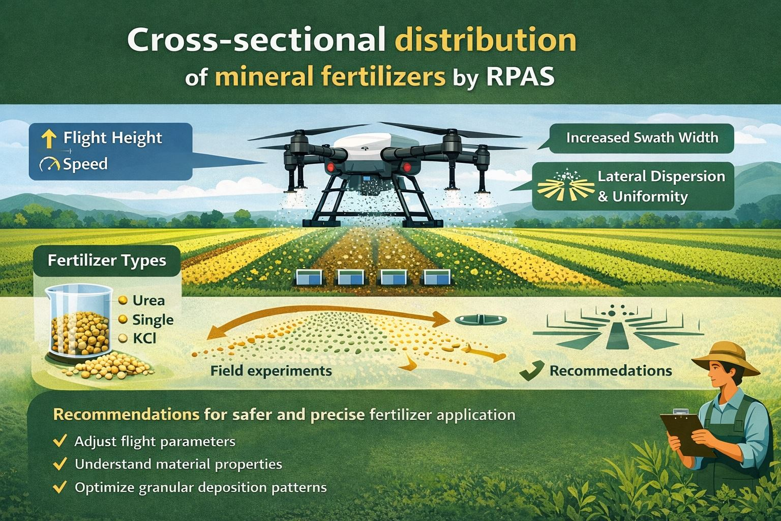
Graphical Abstract

1. Introduction

The Food and Agriculture Organization of the United Nations (FAO) predicts that global food production will need to increase by 70% by 2050 to meet the demand of the world’s population, estimated at 9.7 billion in this period [1,2]. To achieve this goal, it is essential to promote an increase in agricultural productivity and reduce the gap between actual and potential productivity, which can be achieved by adopting efficient practices and technologies. These include proper management of mineral fertilizers and balanced nutrition for agricultural and silviculture crops [3].
The efficiency of this process, however, depends not only on the fertilizer source or dose, but also on the distribution method, which determines the uniformity, precision and, therefore, the effectiveness of the application [4]. Poorly distributed application results in heterogeneous under- or overdosing, reducing nutrient use efficiency, increasing costs and intensifying environmental risks (leaching, volatilization and surface losses) [5,6].
Conventional methods of applying mineral fertilizers include manual practices (broadcast or with backpack applicators), fertigation and mechanized or semi mechanized systems that use helical mechanisms, grooved wheels or gravitational discharge with distribution by centrifugal or pneumatic spreaders [7,8,9]. Although widely used, these systems have operational limitations in areas with uneven terrain, dense crops or obstacles, which can compromise the mobility and uniformity of application, as well as causing impacts such as soil compaction, crop crushing and reduced productivity [10,11].
In extensive cultivation, aerial application with agricultural airplanes and helicopters is a well-established alternative due to its high operational capacity, with solids being dispersed by diffusers (Venturi, Swathmaster or tetrahedral) installed below the hopper [12]. However, this method involves high operating costs, logistical dependence, the need for runways and less precision in small areas or those with complex topography, as well as being directly influenced by aerodynamic flight parameters [13].
In this context, the use of remotely piloted aircraft (RPAs), defined as unmanned aircraft piloted from a remote piloting station and commonly referred to as unmanned aerial vehicles (UAVs) or unmanned aircraft systems (UAS), has been expanding significantly in the agricultural and forestry sectors, being initially consolidated in the application of pesticides and foliar fertilizers in perennial, semi-perennial and annual crops, focusing on the evaluation of the quality of droplet distribution, associated or not with the analysis of biological targets, such as in the control of pests, diseases or weeds [14,15,16,17,18,19,20].
In the context of the dispersal of solid inputs, application with RPAs has evolved from the first applications aimed at sowing rice seeds in China in the early 2000s, to more complex applications of mineral nitrogen fertilization in top dressing, characterized by higher application rates and high operational requirements in wetlands [21,22]. With the advancement of on-board systems, as well as metering mechanisms—gravimetric, grooved wheel/gear and helical—and spreading mechanisms—centrifugal discs and rings, pneumatic systems and distribution devices in lines or strips—[23,24], the use of RPAs has expanded to diverse applications, including direct seeding [25], the application of pesticides in solid formulations [26], assisted pollination [27], the aerial release of biological control agents [28] and the distribution of feed in aquaculture systems [29].
For the application of solid inputs, RPAs offer significant advantages over traditional methods, such as applications on intercropped crops, high operational efficiency, the possibility of localized or variable-rate application regardless of topography, the absence of direct fuel consumption, operation on complex or flooded terrain without the need for airstrips or limitations imposed by the structure of the vegetation [30,31,32,33,34]. In addition, current models have a load capacity of 100–150 kg of solids [35,36,37].
Despite the advances, the application of solid inputs through RPAs still has operational limitations, requiring specialized labor, low battery autonomy and difficulty in ensuring uniform deposition [38,39,40]. These limitations arise from the interaction of multiple factors, particularly the combination of flight operational parameters (flight height and speed, application rate, centrifugal spreader rotation, application swath, and flight path), meteorological conditions, the physical properties of the solid material (relative density, particle size distribution, moisture content, angle of repose, and hygroscopicity), and the characteristics of the dosing and spreading mechanisms employed, all of which affect the deposition pattern and application uniformity [41,42,43,44,45,46,47,48,49,50].
Recent studies have shown that the quality and uniformity of granular fertilizer distribution through RPAs is strongly influenced by the flight operating parameters and the physical properties of the input, affecting the effective application range. The latter, characterized by greater uniformity of granule deposition, is usually assessed by the coefficient of variation (CV), with values of less than 20% considered acceptable for granular fertilizers [51,52].
Song et al. [53] found that the width of the effective range and the CV values are significantly affected by the type of spreading device, with marked differences between centrifugal (disk) and pneumatic systems, as well as by the interaction between height and flight speed in the application of urea. In line with this, Zhou et al. [54] showed that by adjusting the deflector retraction, the rotation of the distributor disk and the flight height, it is possible to achieve a CV of less than 12%, with limited influence from weather conditions and a moderate effect from the airflow generated by the rotors, using the DJI Agras RPA MG-1P model.
In a complementary way, Xia et al. [47] identified that the physical characteristics of fertilizers have a decisive influence on the quality of the application, and their effects are modulated by the height, flight speed and rotation of the centrifugal distributor, in which they observed a 15% increase in productivity in the rice crop using the DJI Agras RPA T40 model. Finally, Wang et al. [55] found that lower flight speeds and smaller particle sizes intensify deposition pattern distortions, while the RPA’s downward airflow reduces the width of the effective application range compared to windless conditions, using the DJI Agras RPA T60 model.
In this sense, the motivation behind this study was to find answers to the theoretical and experimental questions and gaps that still persist in relation to the dispersion of fertilizers by means of RPAs. This study addresses four main gaps: (i) the joint influence of height and flight speed on the distribution of different fertilizers; (ii) the response of physical characteristics to operational variations; (iii) the need for standardized experimental models to assess application uniformity; and (iv) the integration of operational factors and granule properties to predict deposition patterns.
Therefore, the hypotheses raised in this study were: (a) operational flight height and speed are determining factors for the uniformity of mineral fertilizer application through RPAs; (b) lower flight heights tend to generate greater deposition of granules in the effective range, while higher heights expand the total range, reducing application uniformity; (c) higher flight speeds should promote greater lateral dispersion, altering uniformity and increasing the application coefficient of variation; and (d) the physical characteristics of fertilizers significantly influence the distribution pattern when combined with different RPA flight heights and speeds. The aim of this study was to determine the distribution profile of different mineral fertilizers applied by a DJI Agras model T50 remotely piloted aircraft, considering the variability of their physical properties under the influence of different heights and flight operating speeds.

2. Materials and Methods

2.1. Characterization of the Experimental Area

The experiment was conducted at the Experimental Farm of the Centro Universitário Norte do Espírito Santo, of the Federal University of Espírito Santo, located in the municipality of São Mateus-ES, Brazil. The experimental area is located between the coordinates 18°40′25″ S, 40°51′23″ W, on Argissolo type soil with a sandy loam texture. The region’s climate is hot and humid, type Aw, with a dry season in autumn–winter and a rainy season in spring–summer, according to the Köppen classification [56].
For data collection, the experimental area chosen consisted of a large, unobstructed space measuring 5000 m2 (50 m × 100 m), ensuring suitable conditions for the evaluations, without the presence of obstacles that could interfere with the execution of the experimental treatments.

2.2. Characterization of Remotely Piloted Aircraft

A DJI Agras remotely piloted aircraft (RPA) T50 model was used (DJI, SZ DJI Technology Co., Ltd., Shenzhen, China), which has a dual-rotor coaxial structure made up of eight rotors distributed above and below the four swing arms, designed to carry out both spraying and solid dispersion applications. For dispersing solids, the tank has a capacity of 75 L, with an internal load of up to 50 kg, is compatible with solid materials with a diameter of between 0.5 and 5 mm and is equipped with a spiral channel rotating disc, complemented by a deflector that blocks the dispersion of the material, preventing damage to the propellers.
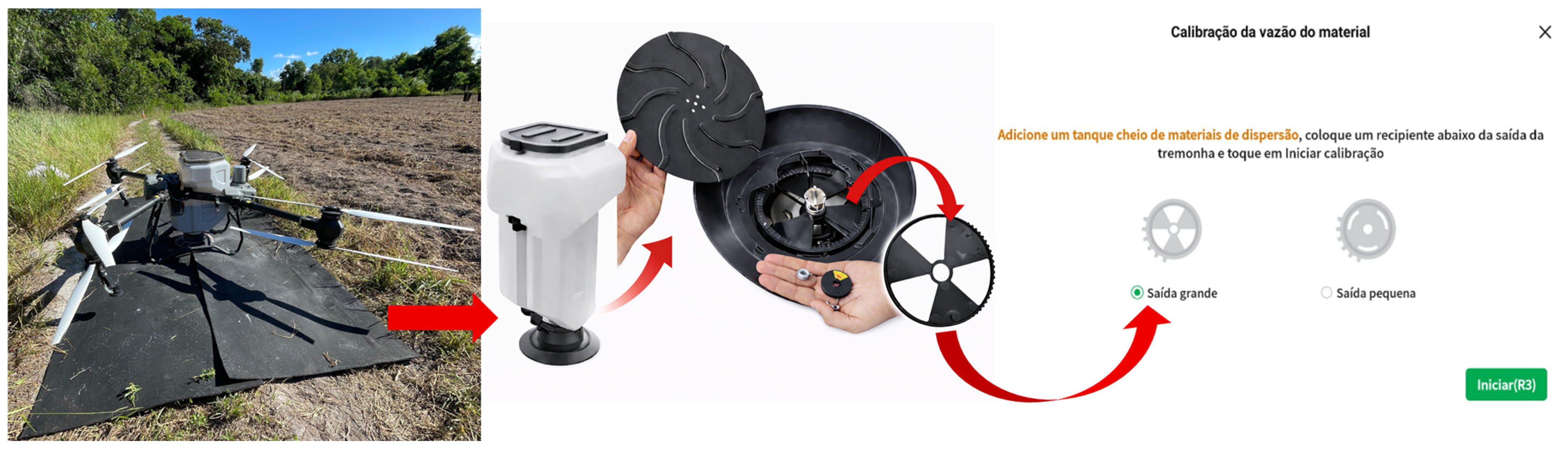
This RPA has a quick release device in the hopper, which allows precise adjustments according to the flow of material to be dispersed and the diameter of the granules. In all the experimental treatments, the outlet of the hopper with the largest capacity was used, as indicated by the manufacturer for higher volume applications [57]. The setting was selected on the RPA’s radio control during the calibration process, as recommended by the manufacturer for applications at higher application rates (kg ha−1) (Figure 1).

2.3. Determination of Physical Characteristics of Mineral Fertilizers

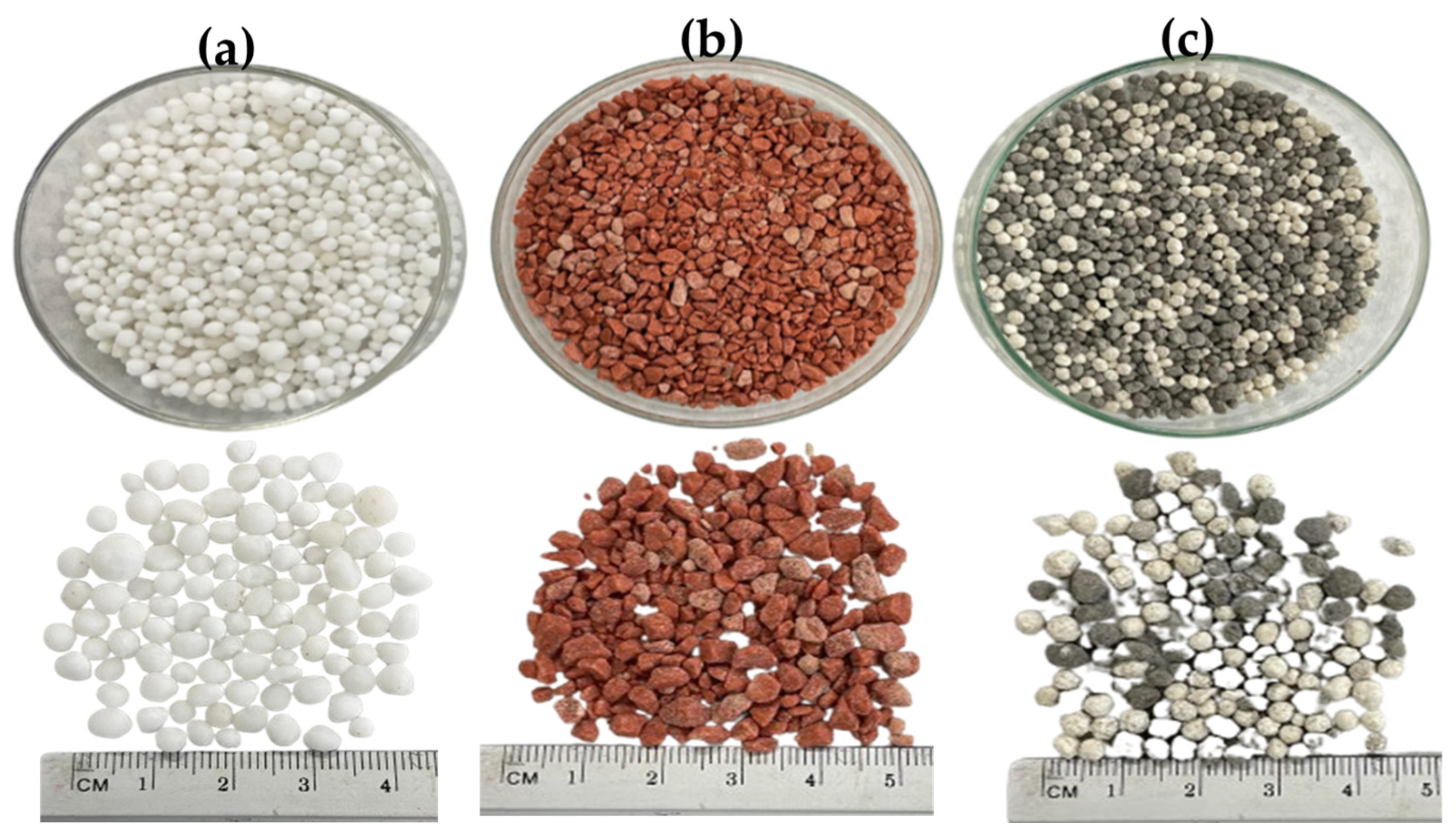
Three commercial granular mineral fertilizers were used alone (without mixing): simple superphosphate (18% P2O5, 16% Ca and 10% S), granulated urea (46% N) and granulated red potassium chloride (60% K2O) (Figure 2). The choice of these fertilizers is justified by their widespread use in N–P2O5–K2O mineral fertilization practices, both in agriculture and silviculture. The aim of this stage was to characterize the average values of the main physical properties, which were then used in the correlation analyses (Section 2.6—Statistical analyses) and the results are presented in Appendix A.1.
To determine the physical characteristics, four 500 g samples of each mineral fertilizer were randomly collected directly from the commercial packages, which were packed in airtight plastic bags to avoid physical and hygroscopic changes and then sent to the laboratory for analysis. The initial samples were homogenized and divided into sub-samples for the experimental replicates. Six replicates of 100 g per fertilizer were used for the analyses of the granule dispersion index, percentage of granules ≤ 106 µm, water content and relative density. For the angle of repose, six repetitions of 4 kg per fertilizer were used. Sphericity was determined from granules collected at random in each repetition of the previous analyses.
The Granule Dispersion Index (GSI) was determined according to the Manual of Official Methods for Fertilizers and Correctives [58], using standardized sieves (3.55 mm to 63 µm). Samples of 100 g were shaken for 10 min, and the retained fractions were weighed to calculate the percentage distribution and the GSI; the fraction ≤ 106 µm was expressed as the percentage by mass of the material passing this sieve. The water content was determined according to Alcarde et al. [41], by drying sub-samples at 50 °C for 48 h until constant mass, and calculated by the percentage difference between the wet and dry masses. The relative density was obtained in accordance with ISO 3944:1992 [59], using 100 g of sample transferred without compaction to a graduated cylinder, calculated using the mass/volume ratio (g cm−3).
The angle of repose was determined according to Reynaldo [60], by forming a mound in a glass box, and the angle was calculated trigonometrically from the height and radius of the base of the cone formed. Finally, sphericity was measured in 100 intact granules per fertilizer, by measuring the triaxial dimensions (length, width and thickness) using a digital caliper (0.001 mm), calculated by the ratio between the equivalent diameter and the length of the granule, according to Sun et al. [61]. The formulas used to calculate each variable are shown in Table 1.

2.4. Determination of the Cross-Sectional Distribution Profile of Mineral Fertilizers

The cross-sectional distribution profile was evaluated by collecting the fertilizers in the field. However, as this was an experiment conducted with the DJI Agras T50 RPA (DJI, SZ DJI Technology Co., Ltd., Shenzhen, China), some methodological adaptations were necessary, as suggested by Zhang et al. [62], Liu et al. [46] and Wang et al. [55] in the distribution of fertilizers. The adaptations involved reducing the number of collectors, adjusting the distances between them and changing the dimensions of the collectors, without compromising the reliability of the experimental results.
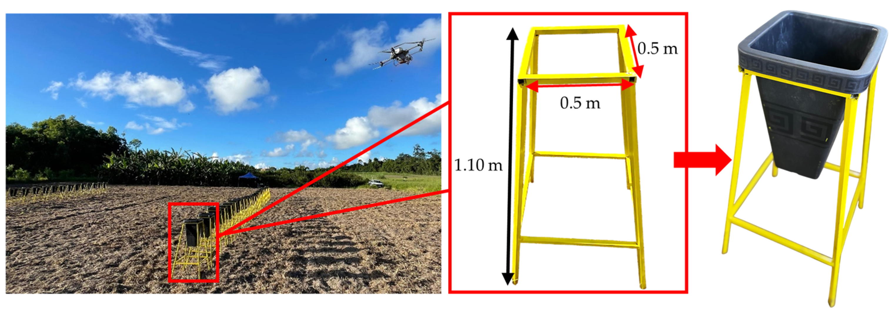
To collect the fertilizers, 50 pyramid-shaped polyethylene collectors were used, measuring 34.50 cm high × 34.50 cm wide × 52.10 cm long. Galvanized metal structures painted safety yellow, measuring 1.10 m high × 0.50 m wide, were made to keep the collectors standardized and structured at a height of 1.0 m above the ground in the experimental area (Figure 3), in order to withstand the wind generated by the RPA’s propellers.
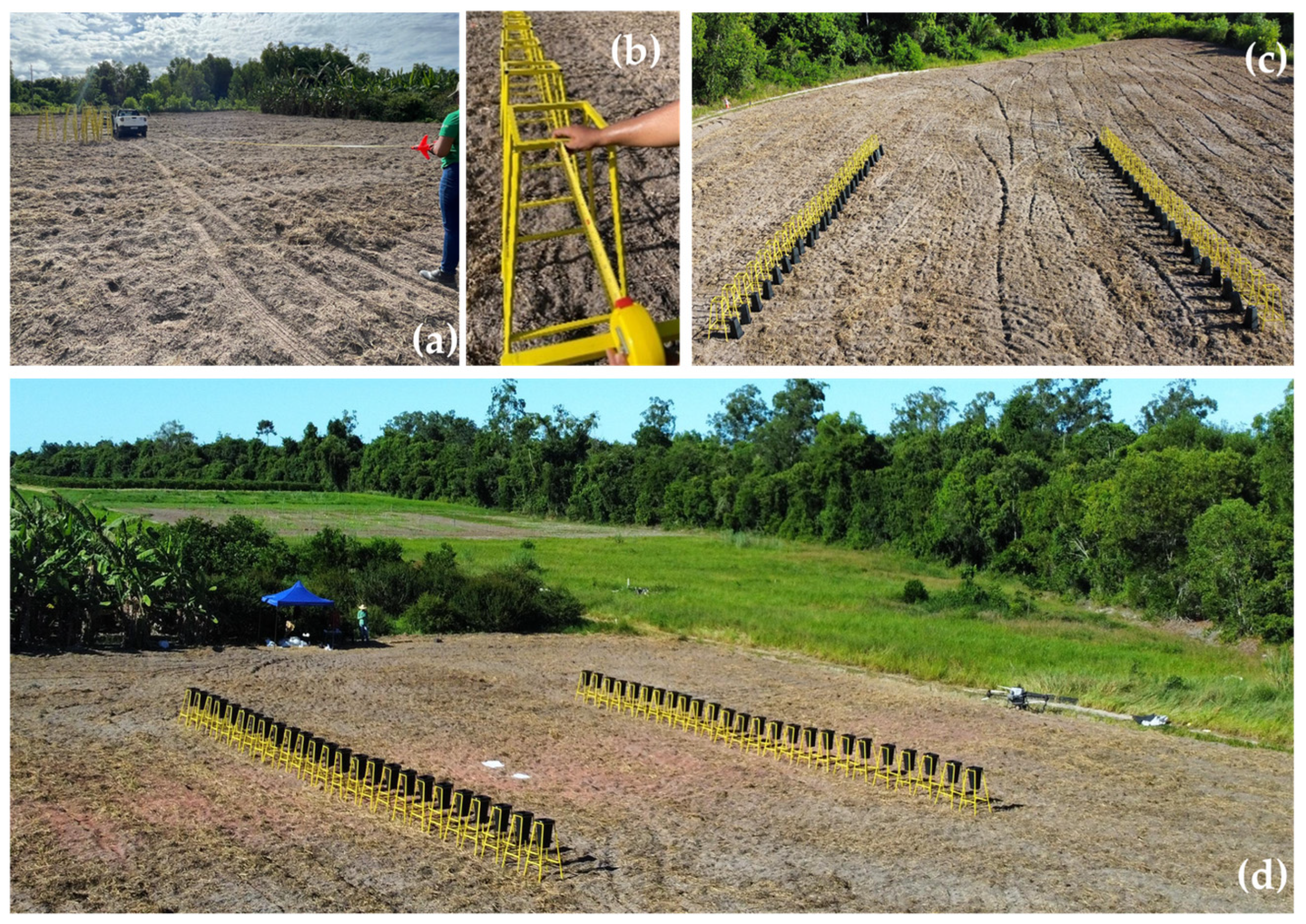
Before the experimental treatments were applied, the structures and collectors were tested in the field to check for any ricocheting of particles after impact. No effects were observed, which validated the use of these structures for the collection stages of the experimental treatments.
Before each application, each mineral fertilizer was calibrated individually in the RPA. The distribution system’s rotating disk was removed to keep the outflow in a fillet, allowing the material to be collected and returned to the bag. For the ground calibration, the aircraft was supported on boxes and kept at a height of approximately 40 cm from the ground. Initially, calibration was carried out with an empty tank, followed by checking the Hall effect and weight sensors. At the start of each experimental day, 45 kg of fertilizer was inserted into the tank, selecting the large outlet opening according to the physical characteristics of the material, and the calibration was carried out automatically by the on-board system.

2.4.1. Experimental Design

This stage was carried out separately for each mineral fertilizer evaluated (simple superphosphate, urea and potassium chloride). The experiment was structured in a randomized block design with a 3 × 3 × 3 factorial scheme: three fertilizers (simple superphosphate, urea and potassium chloride), three flight heights (4, 6 and 8 m) and three speeds (16, 18 and 20 km h−1), with four repetitions. The 27 experimental treatments were previously configured in the RPA control system before each application.
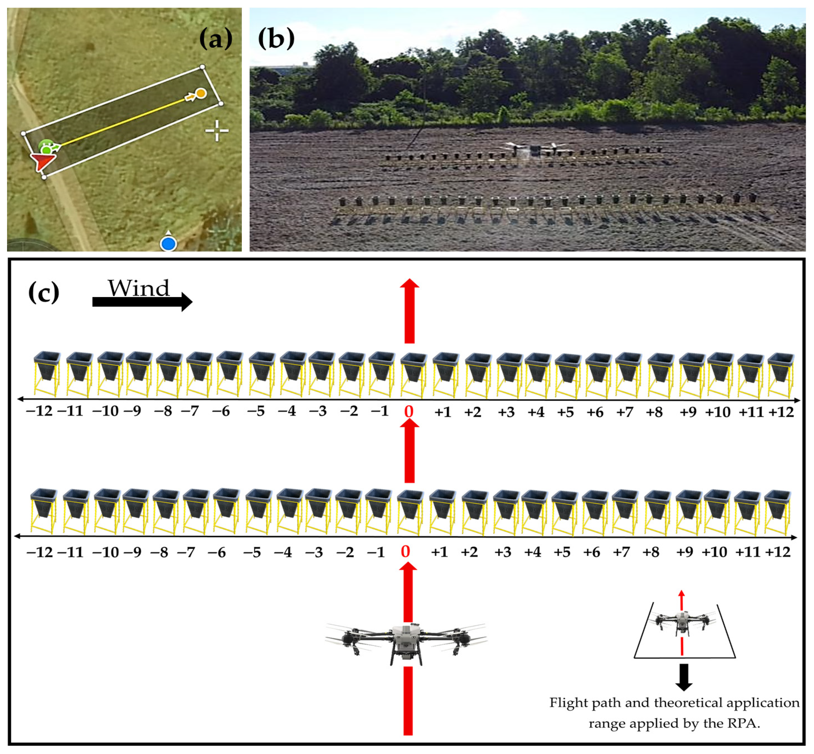
Each repetition corresponded to one day of application, with the variation between blocks represented by the different days of application, applied at the same times. The treatments were standardized in order to guarantee the sources of variation established in the study. The following operating parameters were previously adjusted in the RPA control and kept constant for all treatments: theoretical application range of 8 m and centrifugal disc rotation of 800 rpm as suggested by Wang et al. [22]; application rate of 400 kg ha−1, aiming for greater collection volume; and flight path perpendicular to the wind direction, as recommended in RPA operations [63].
In the experimental area, with a tape measure, the structures equipped with the collectors were distributed in two parallel lines, spaced 15.0 m apart, with 25 units in each line, arranged 0.50 m apart (Figure 4). The lines with the collectors were previously identified (1 to 25) and aligned with the prevailing wind direction and perpendicular to the direction of the RPA’s flight path. The treatments were carried out on a total area of 5000 m2 (50 m × 100 m); however, the useful area of the experimental unit (area occupied by the collectors) was approximately 375.0 m2 (15 m × 25 m).
Considering the 27 experimental treatments and four replications (blocks, represented by the application days), the experiment totaled 108 experimental units. Each experimental unit corresponded to one flight and was composed of two subsamples (collection lines), whose values were later converted into means for statistical analyses (Topic 2.6. Statistical analysis). The application was started approximately 20 m before the collector line in order to activate the centrifugal disc, stabilize the height and flight speed, and start spreading the fertilizer.
In the RPA control system, the theoretical application range was kept at 8 m for all treatments, and the aircraft only covered one route line. This procedure made it possible to determine the total range and the effective range of application, isolating the performance of the spreading system according to the characteristics of each fertilizer, without interference from overlaps. This approach is fundamental for accurately assessing the lateral distribution of fertilizers applied by RPAs [39]. Figure 5 shows the experimental scheme used.
After the application of each treatment, the fertilizer deposited in each collector was removed using a brush and transferred to collection containers, identified according to the sampling point and packed in double zip-lock plastic bags with airtight seals. They were then immediately sent to the Laboratory of Mechanization and Agricultural Defensives (LMDA) at the North University Center of Espírito Santo, Federal University of Espírito Santo, in São Mateus ES, Brazil.
In the laboratory, the samples were transferred to Petri dishes and weighed on a precision analytical balance (0.001 ± 0.001 g). The same collection points were used in all experimental replications, ensuring that the final averages per collection line were obtained at the end of the experiment.

2.4.2. Variables Relating to the Total Application Range

The sum of the granule deposition in the total range was calculated from the sum of the individual fertilizer depositions in each collector distributed along the total application width, in which the presence of non-zero granules was recorded, expressing the results in grams per square meter. The width of the total application range was defined as the total transverse distance at which the presence of granules in the collectors was observed, with non-zero deposition. The equations relating the variables of the total application range are shown in Table 2.

2.4.3. Response Variables for the Effective Application Range

The coefficient of variation (CV) was adopted as a statistical measure for assessing the uniformity of application distribution over the effective application range [64]. To do this, simulations of successive overlays were carried out based on the accumulated deposition values in the collectors, with the CV calculated for each simulated overlay condition according to studies carried out by Song et al. [52] and Wang et al. [22,55] using RPAs for mineral fertilization.
The analyses were carried out using the software Adulanço® version 4.0 [65], developed by the Mechanization and Precision Agriculture Group (GMAP) of Escola Superior de Agricultura Luiz de Queiroz at the University of São Paulo (ESALQ/USP, Brazil) [66], which allows successive overlays to be simulated in order to calculate the coefficient of variation. Similar studies have used Adulanço® to analyze the cross-sectional distribution of fertilizer and corrective applicators [5,67,68,69].
The software made it possible to simulate three application systems: an alternating system (right and left) and a continuous system. In this study, for the following variables related to the effective application range, the continuous system was adopted, as it simulates the overlap between the right and left sides of the machine’s deposition, and vice versa, minimizing possible imbalances resulting from asymmetry in the deposition pattern [70,71]. This procedure more realistically represented the operating conditions of the study, in which the back-to-back route system, commonly used in commercial operations with RPAs, is predominantly used [13].
For each overlap width considered in each experimental treatment, the software recalculated the accumulated transversal distribution along the application range and determined the coefficient of variation (CV) of the deposition. Based on these simulations, the effective application range was defined as the greatest width with a CV ≤ 20%, a value widely adopted for granular fertilizers [72,73]. Based on the width of the effective range identified in each treatment, the collectors located within the lateral limits of this range (±width/2 in relation to the center of the application range) were selected, from which the response variables shown below were determined.
The average deposition of granules in the effective range was determined by the arithmetic mean of the depositions recorded in the collectors located within the limits of the effective range, according to Song et al. [53]. The effective range width was defined as the maximum cross-sectional length of the application with a CV ≤ 20%.
Based on the effective width and operational flight speed of each treatment, the theoretical operational capacity of the effective range was estimated, according to Antuniassi and Boller [74], with the unit adapted to ha h−1. As this is a theoretical estimate, operating losses, maneuvers, overlaps, interruptions or unproductive times were not taken into account, as discussed by Ferreira and Matuo [75]. The equations relating the variables of the effective application range are shown in Table 3.

2.4.4. Application Efficiency and Relative Error

Application efficiency was determined as the ratio between the deposition retained in the effective range and the total deposition collected in the application range, expressing the fraction of fertilizer effectively used and the lateral losses associated with the process (Table 4). The relative error, considered in this study as the relative error of the total mass deposited, was used to quantify the percentage deviation between the amount of fertilizer actually deposited and the programmed theoretical dose, based on an adaptation of the equations proposed by Su et al. [6] and Zhou et al. [54] as described in Table 4.

2.5. Monitoring Weather Conditions

All the experimental treatments were applied in the afternoon between 1:00 PM and 4:00 PM. Throughout the experiment, relative humidity, air temperature, wind speed, direction and average gust were recorded automatically at hourly intervals. This information was obtained from the automatic weather station model A616 of the National Institute of Meteorology (INMET), manufactured by Vaisala® (Vantaa, Uusimaa, Finland), equipped with various internal and external sensors, located approximately 650 m from the experimental area. Table S1 shows the complete meteorological data for each day of application.

2.6. Statistical Analysis

Initially, the averages of two independent groups regarding the deposition of granules (g) in the collection lines (Line 1 and Line 2) were compared using Student’s t-test for two independent samples, assuming equivalent variances, for each experimental treatment involving the fertilizers evaluated—urea (Table S2), potassium chloride (Table S3) and simple superphosphate (Table S4). There were no statistically significant differences between the means (two tailed p-value > 0.05). Once this assumption had been met, the data from both lines was grouped and converted into average values, which were then used to analyze the variables associated with the total application range and the effective application range.
The variables related to topic 2.4 (Determination of the cross-sectional distribution profile of fertilizers) were previously assessed for compliance with the assumptions of the analysis of variance. Next, the variables related to the total application range, effective application range, application efficiency and relative error were submitted to analysis of variance (Appendix A.2) and when significant differences were identified, the means were compared using the Tukey test, adopting a significance level of 5%.
The association between the variables obtained in topics 2.3 (Determination of the physical characteristics of fertilizers) and 2.4 (Determination of the transversal distribution profile) was estimated by means of Spearman’s correlation, using its coefficient (Spearman’s rho—ρs) to interpret and classify the results, considering the guide proposed by Mukaka [76]. The choice of this method was justified by the lack of normality of some variables, even after applying transformations to the data (logarithmic transformation [log (x + 1)] for variables containing zero values and [log(x)] for strictly positive variables). In addition, Spearman’s coefficient does not assume normality or a strict linear relationship, but is based on the ordering of values (ranks), which makes it more robust to the presence of extreme values (outliers).
Different graphic resources were used to present the results of the analyses described above, including bar and scatter graphs, violin-type boxplots and heatmaps, allowing integrated visualization of the trends and relationships between the variables evaluated. All statistical analyses and the preparation of graphs were carried out in the RStudio software version 4.5.0 [77], using specific packages appropriate to each analytical procedure.

2.7. Artificial Intelligence Tools

In the development of this study, tools based on artificial intelligence were used as auxiliary support in specific stages of the research. The Litmaps and LeapSpace platforms were used to systematically prospect, organize and map scientific literature, making it possible to identify relationships between studies, gaps in knowledge and trends regarding the subject of the study. In addition, the DeepSeek V3 and ChatGPT 5.2 tools were used to support the conceptual organization of the content, to improve textual clarity, cohesion and precision and to review the computational scripts of the statistical analyses, including suggestions for optimizing and standardizing codes. It should be emphasized that the use of these tools was exclusively auxiliary and did not replace the critical analysis of this study.

3. Results

3.1. Variables Related to the Total Application Range

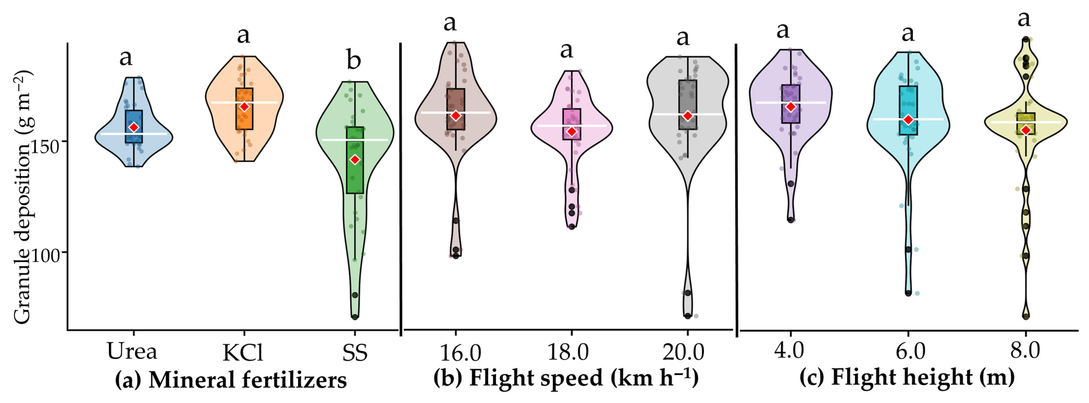
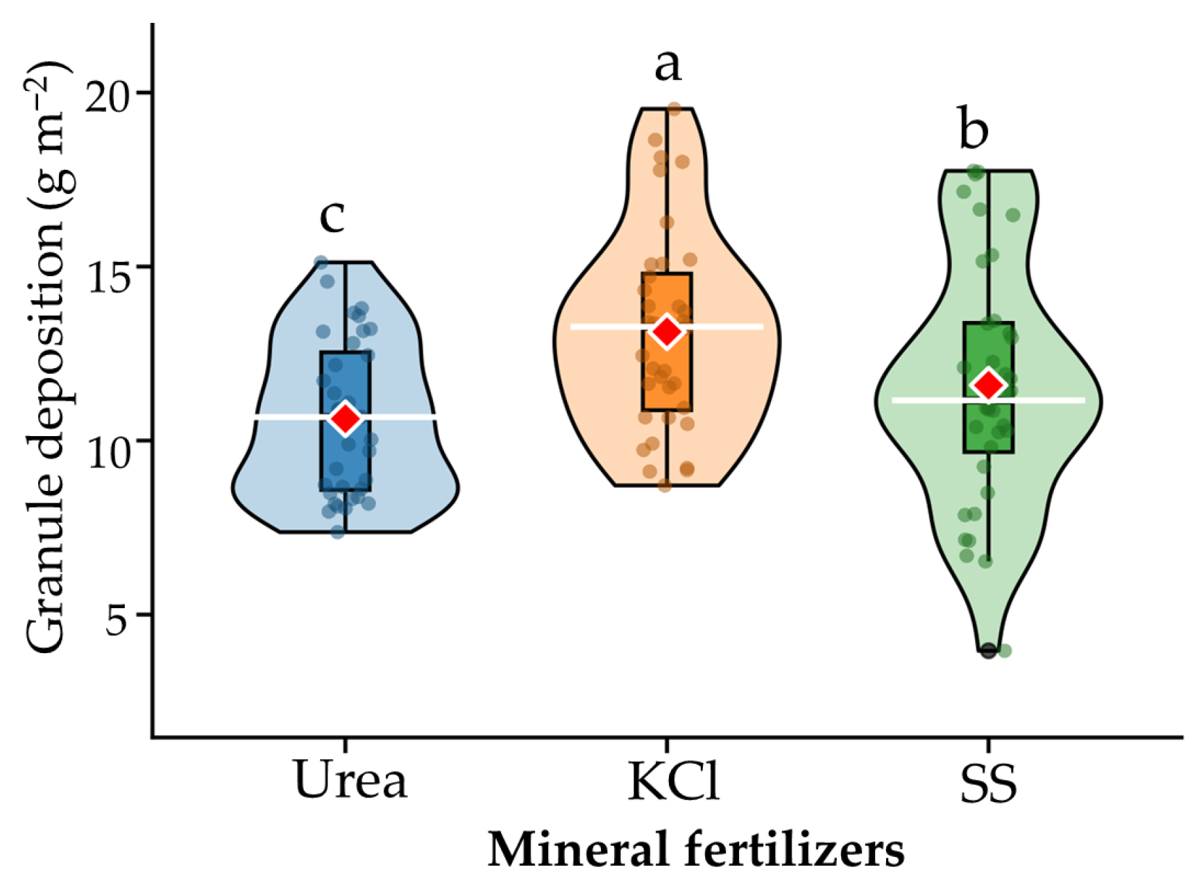
The sum of the deposition of granules in the total range was significantly influenced by the type of mineral fertilizer and was not affected by height or flight speed alone (Figure 6; Appendix A.2). In general, there was a consistent trend towards greater deposition of granules within the total range for potassium chloride (KCl), followed by urea—statistically similar—and, lastly, simple superphosphate (SS). KCl showed significantly higher deposition, being 5.63% higher than urea and 14.42% higher than SS, within the total application range.
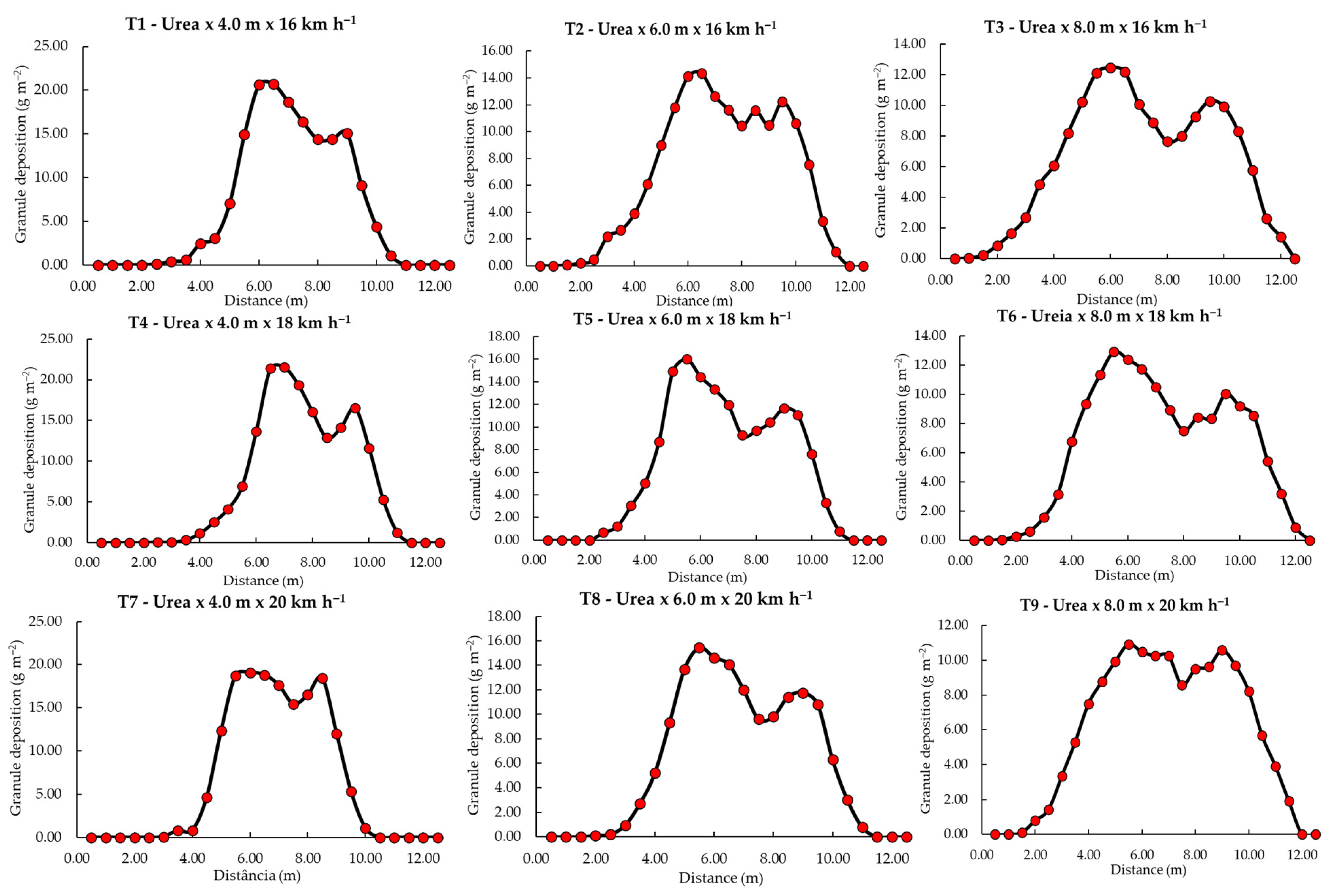
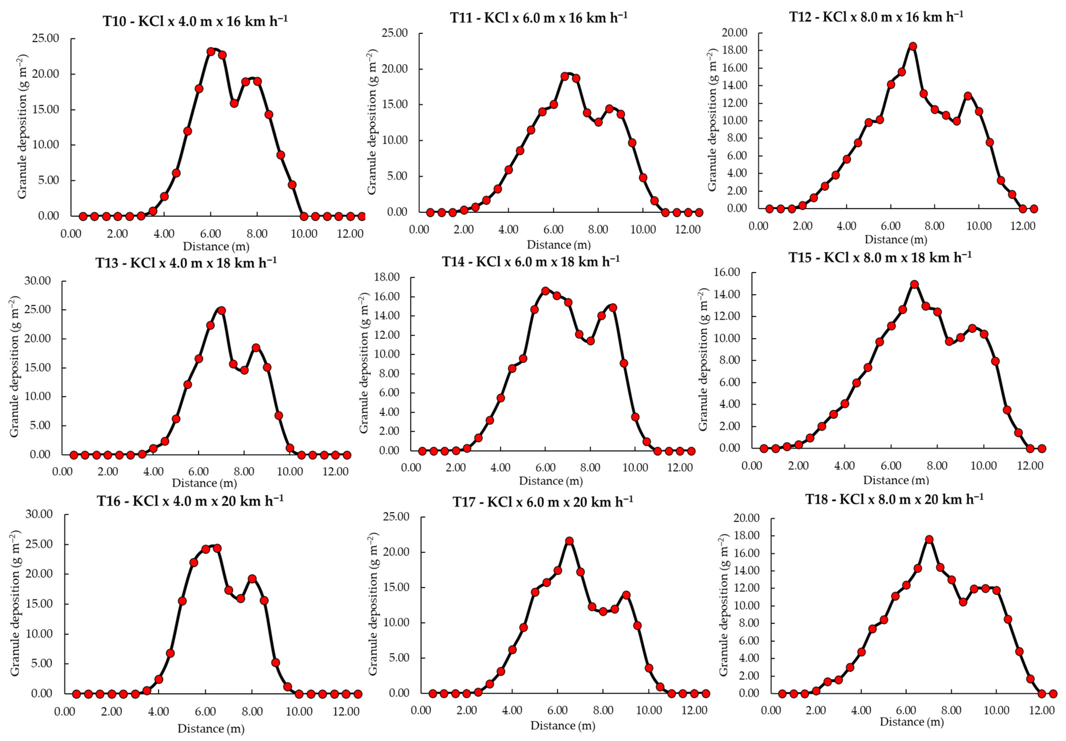
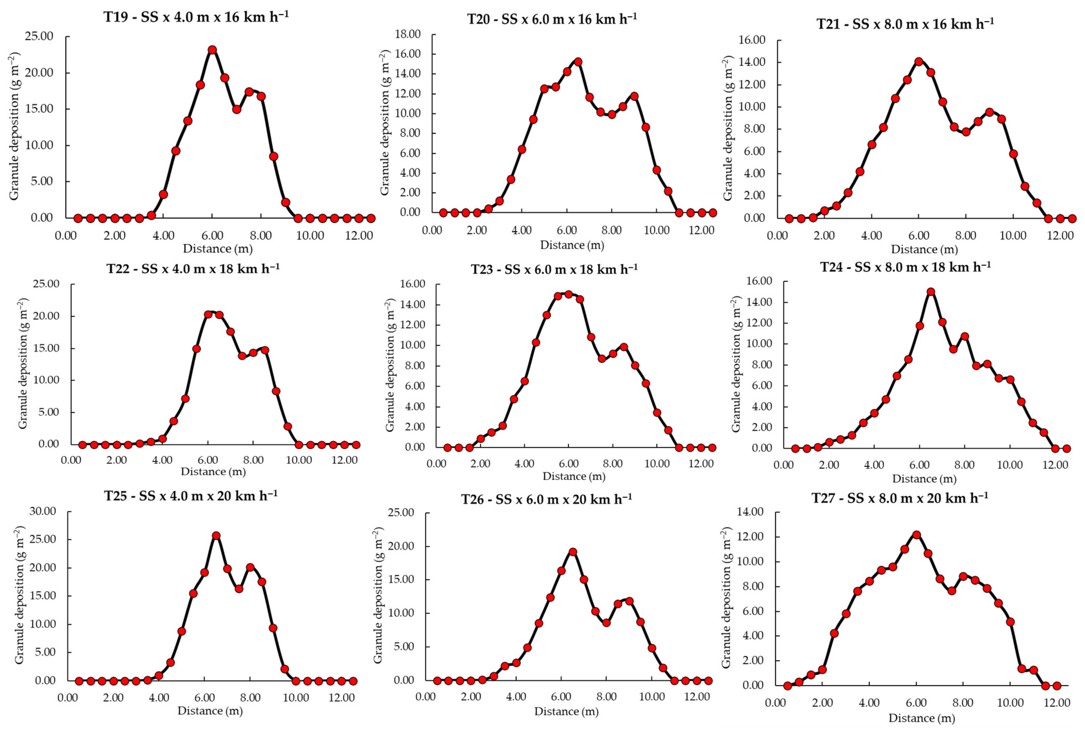
Although the total mass deposited did not vary with height or speed alone, the width of the total range of application responded strongly to the three-way interaction between the fertilizer, height and speed factors (Table 5; Appendix A.2). Urea showed the greatest total range width, regardless of the flight parameters. 16 km h−1 and 6 m high, the application range was 10.5 m (urea), 9.0 m (KCl) and 8.5 m (SS), representing differences of 14.28% in relation to KCl and 19.04% in relation to SS. This pattern was repeated in all operating combinations, showing greater lateral dispersion of the urea.
The effect of speed depended on the fertilizer and height (Table 6). For KCl, the variation between 16 and 18 km h−1, there was little change, especially at heights of 4 and 6 m, with no statistical difference. For simple superphosphate, the influence was reduced, with differences between 18 and 20 km h−1 at 4 and 6 m and no differences at 8 m. For urea, there was greater variation: at 4 m it increased between 16 and 18 km h−1, reducing at 20 km h−1; at 6 and 8 m, the differences were smaller.
In general, for all fertilizers, increasing the flight height from 4 to 8 m led to a significant increase in total range, regardless of flight speed. On the other hand, increasing the flight speed to 20 km h−1 resulted in a slight reduction in the width of the total range, especially for KCl and urea at the lowest flight heights, although this reduction was less than 1.0 m in most combinations (Table 5). The joint analysis of the granule distribution profiles along the total range (Figure 7, Figure 8 and Figure 9) confirms that flight speed acted as a secondary factor in relation to flight height, modulating the response of each mineral fertilizer, with urea being more sensitive to operational variations.

3.2. Variables Related to the Effective Application Range

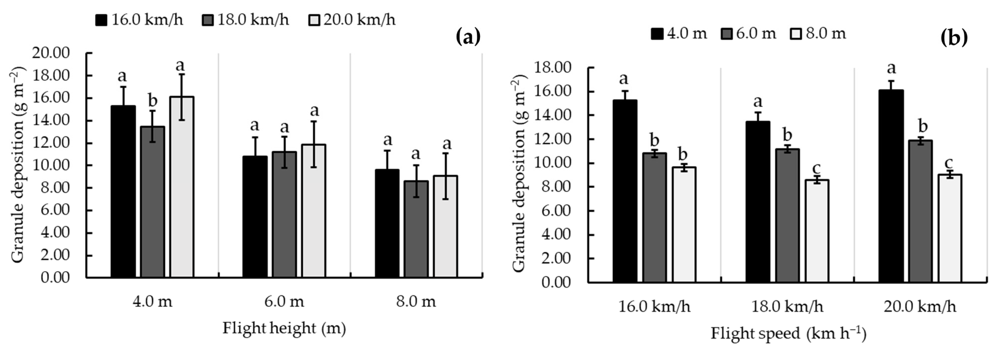
Deposition in the effective range was influenced by the interaction between height and operational flight speed (Figure 10; Appendix A.2). Speed had a less pronounced effect than height (Figure 10a). At 4 m, the greatest deposition occurred at 20 km h−1, 5% higher than at 16 km h−1 (similar) and 16.3% at 18 km h−1 (different). At 6 and 8 m there were no statistical differences between speeds, restricting the effect to the lower heights.
Deposition in the effective range decreased consistently with increasing height (Figure 10b). At 4 m, the highest values were recorded; at 6 m, an intermediate decrease; at 8 m, lower results between 8.61 and 9.63 g m−1. Raising the height from 4 to 8 m led to a reduction of more than 35% in average deposition, regardless of speed.
The average deposition of granules in the effective range differed significantly between fertilizers, regardless of height and flight speed (Figure 11). Potassium chloride (KCl) had the highest average deposition value, followed by simple superphosphate and urea. There was also greater dispersion of the data for simple superphosphate, evidenced by the greater amplitude, while KCl showed a more concentrated distribution around the average, indicating greater regularity in deposition.
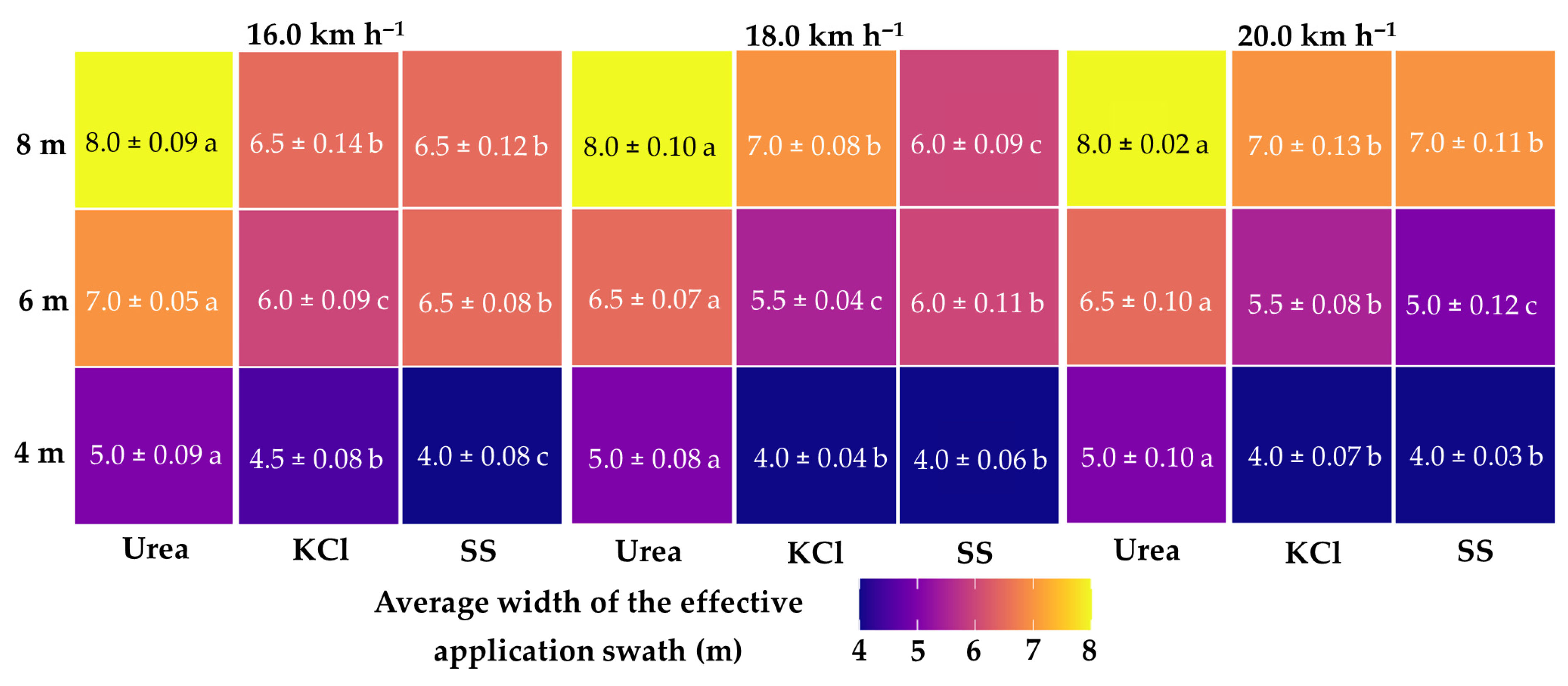
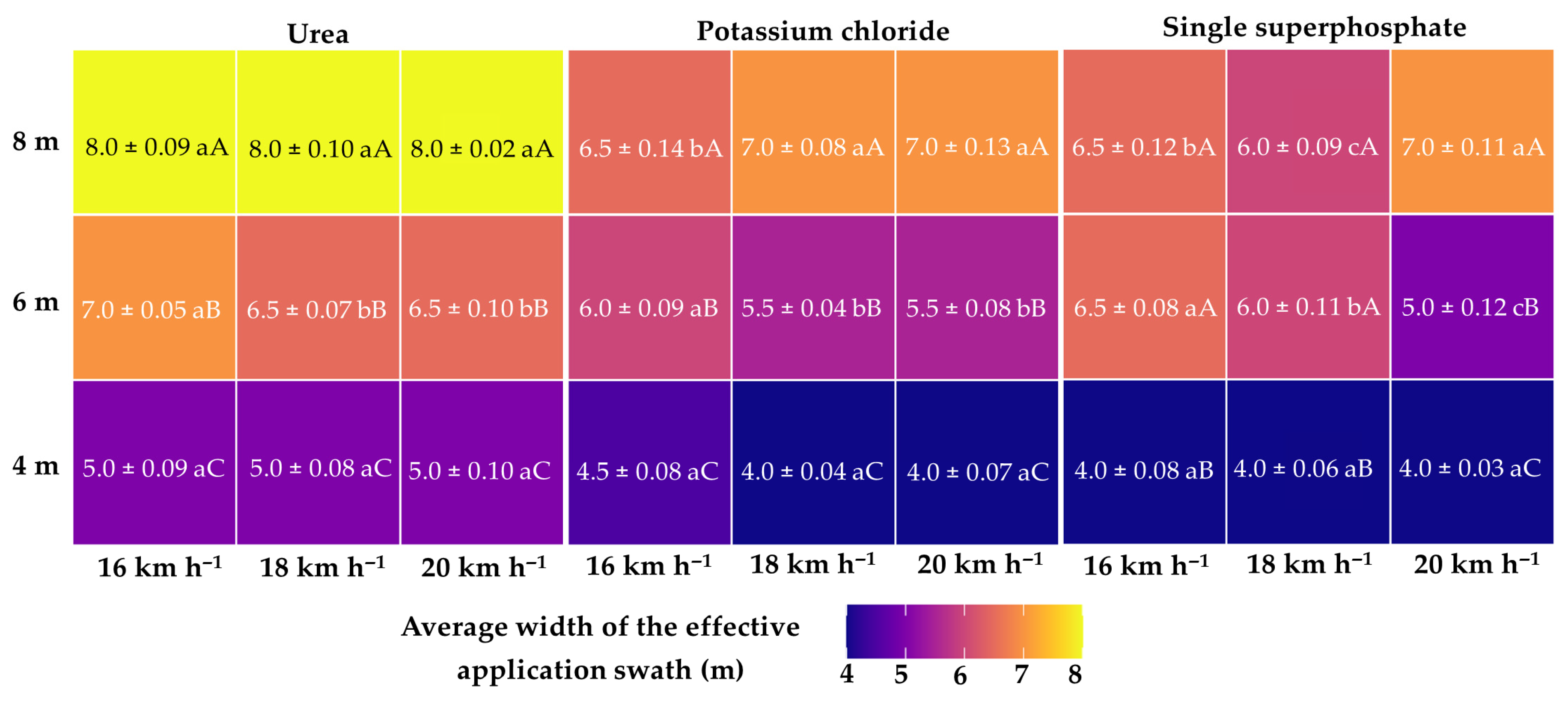
The effective range was influenced by the interaction between fertilizer, height and operational flight speed (Figure 12; Appendix A.2). Height increased significantly from 4 to 8 m in most combinations. Urea showed higher values than the other fertilizers. Speed only promoted specific variations in height, with differences restricted to specific combinations, without altering the order between fertilizers. A similar trend was observed for the width of the total application range (Table 5).
When analyzing each mineral fertilizer separately, different operational behaviors were observed (Figure 13). For urea, the width of the effective range was determined predominantly by flight height, with a significant increase of approximately 37.5% when raising the height from 4 to 8 m, while speed did not alter this pattern, with no statistical differences between 16 and 20 km h−1 within each flight height. For potassium chloride, flight height also significantly widened the range, but flight speed began to modulate the response at higher flight heights: at 6 m, increased speed significantly reduced the width, while at 8 m, the range increased with increased flight speed. Simple superphosphate, on the other hand, showed greater variability between operational combinations, with significant reductions in some conditions—such as at 6 m at 20 km h−1—indicating greater sensitivity between the operating conditions evaluated.
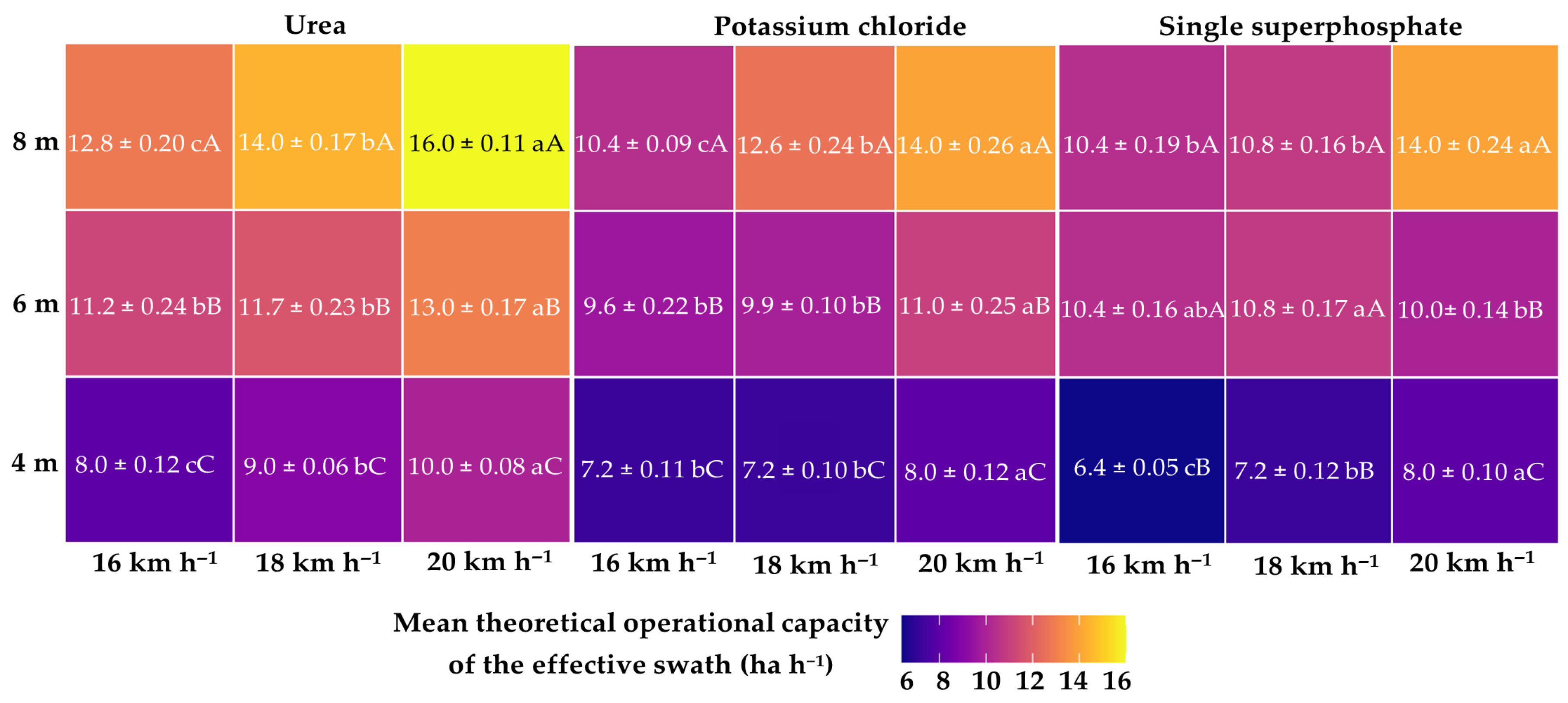
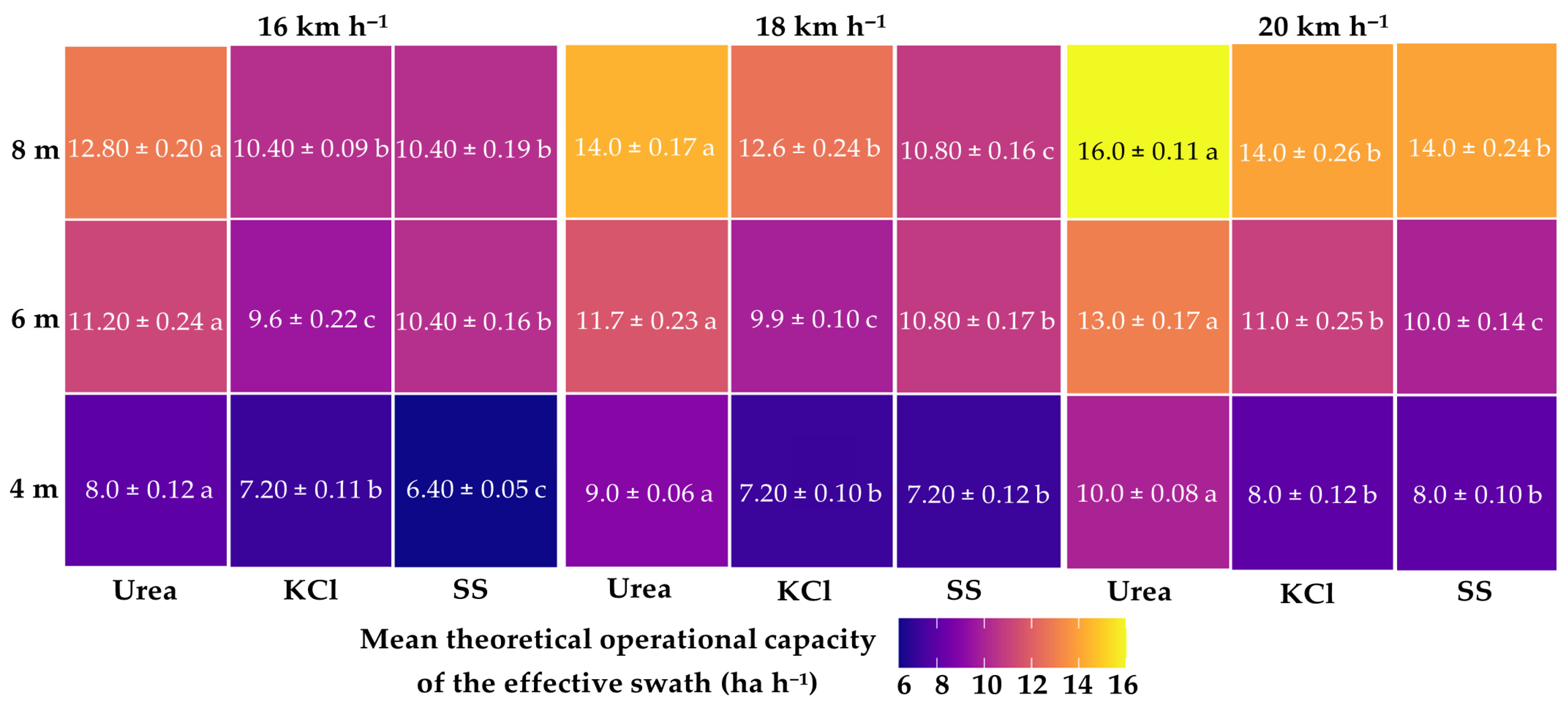
The theoretical operating capacity of the effective range was significantly affected by the interaction between mineral fertilizer, height and flight speed (Figure 14; Appendix A.2). It was observed that the lowest values were concentrated at a flight height of 4 m, while raising the height to 8 m led to a consistent increase in operational yield, reaching up to 16.0 ha h−1 for urea at 20 km h−1. The effect of speed became more evident at greater heights: at 8 m, the transition from 16 to 20 km h−1 resulted in increases of around 20% for urea and around 25.7% for simple superphosphate. In practically all operational combinations, urea had the highest capacities, followed by potassium chloride and simple superphosphate.
When analyzed separately, the fertilizers showed different responses (Figure 15). For urea, the variation in flight height was the main determinant of performance, establishing three well-defined operational levels (4 < 6 < 8 m), while flight speed only extended the values within each range. With potassium chloride, in addition to the effect of flight height, flight speed made an additional contribution, especially at 8 m, where the difference between 16 and 20 km h−1 reached approximately 3.6 ha h−1. Simple superphosphate showed the lowest performance at the lowest flight heights, but gradually increased under higher conditions, especially at 20 km h−1, confirming different responses between the fertilizers under the same operating conditions.

3.3. Variables Related to Application Efficiency and Relative Application Error

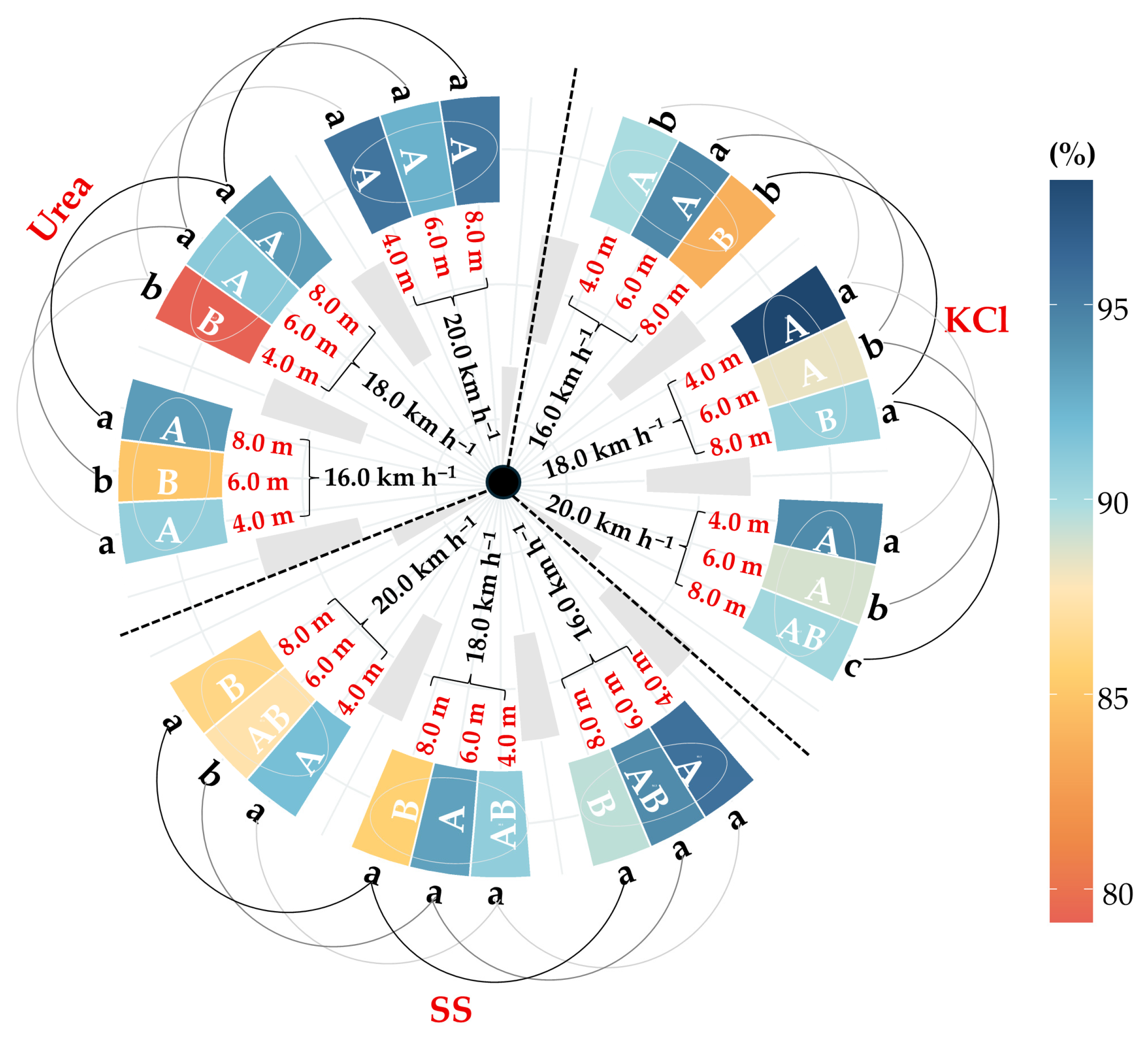
The application efficiency showed an interaction among mineral fertilizer, flight height, and flight speed (Table 7; Appendix A.2). This interaction revealed wide variability among fertilizers, with no consistent linear trend. At 16 km h−1, single superphosphate (SS) showed the highest efficiency at 4 m, with a progressive reduction as height increased. At 18 km h−1, KCl showed the best performance at 4 m, whereas urea presented increasing values with increasing height. At 20 km h−1, differences occurred only at 8 m, establishing the following order: urea > KCl > SS.
The circular heat map (Figure 16) confirms the pattern observed in the breakdown of the triple interaction (Table 7), indicating that application efficiency depends on the simultaneous adjustment of flight height and flight speed. Urea showed the highest application efficiency at 20 km h−1, regardless of flight height. Potassium chloride exhibited greater contrast among the operational combinations, with the highest efficiencies concentrated under intermediate conditions and showing an inverse relationship with flight height at 16 km h−1. For single superphosphate, greater spatial heterogeneity was observed, with a significant trend of gradual decrease in application efficiency as flight height increased, particularly at flight speeds of 16 and 20 km h−1.
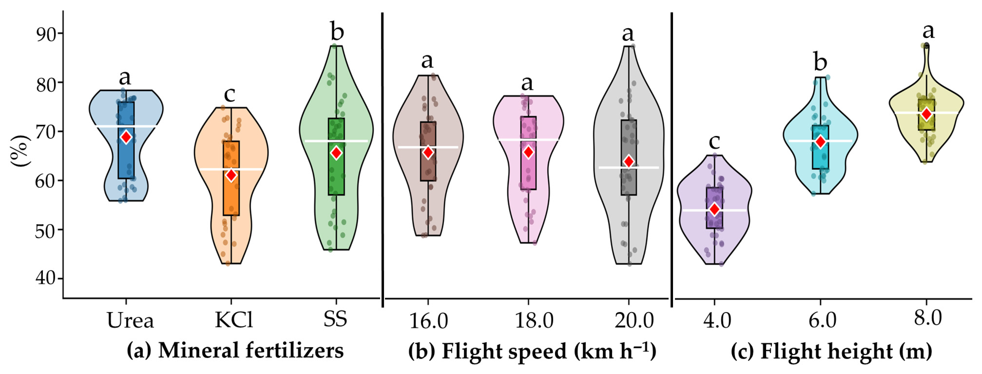
The relative error of the total mass of granule deposition showed no triple interaction among the evaluated factors (Figure 17; Appendix A.2). For fertilizers (Figure 17a), the following significant order was observed: urea > single superphosphate > KCl. For the flight speed factor (Figure 17b), no statistical differences were detected among the evaluated speeds. Flight height significantly influenced the relative error of the total mass (Figure 17c), showing a directly proportional relationship: as height increased, the error also increased. Specifically, the 4 m condition presented the lowest mean values, whereas increasing the height to 8 m resulted in an increase of approximately 19.3% compared to the lowest height.

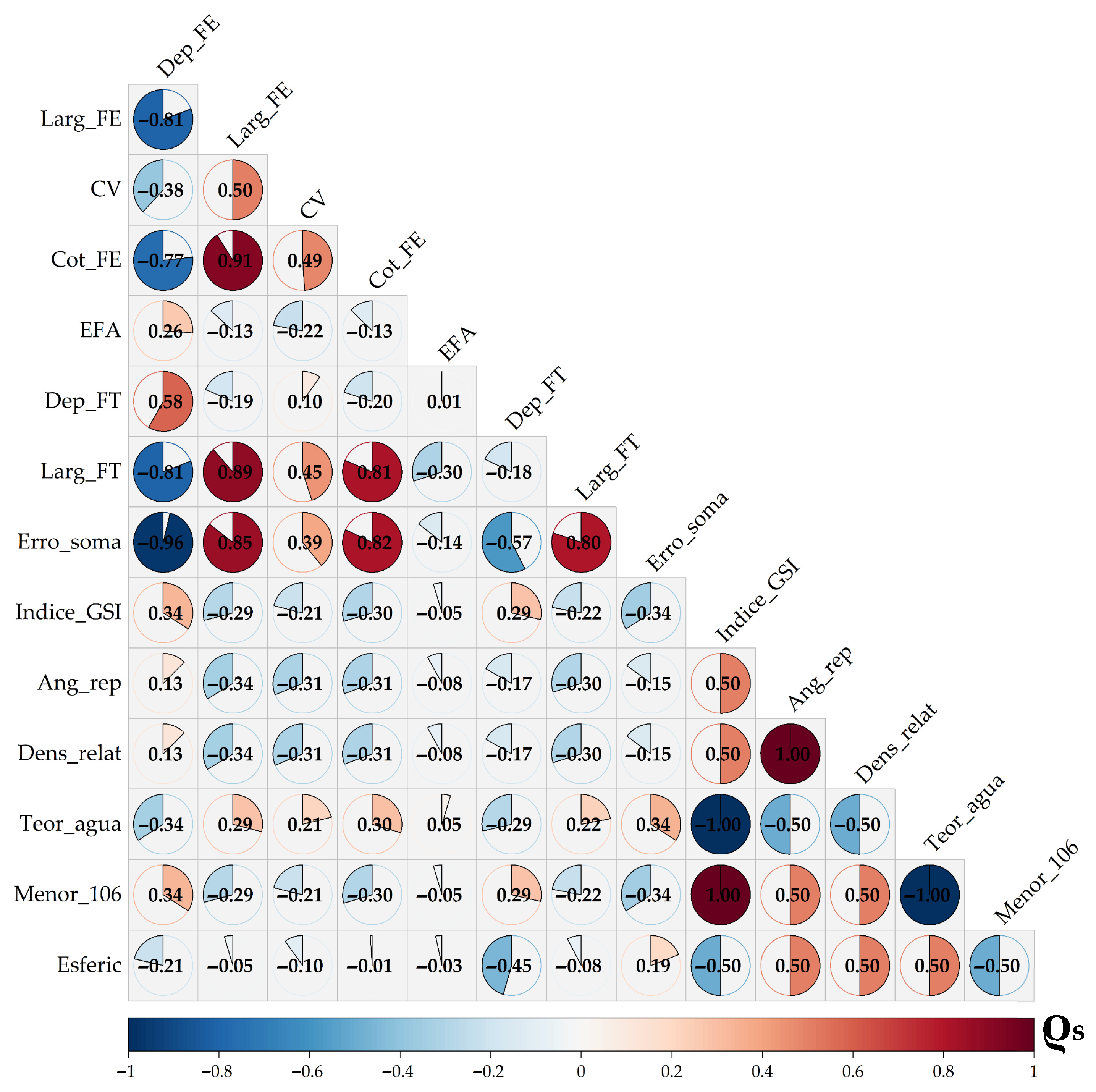
3.4. Spearman Correlation Between the Variables

The Spearman correlation analysis (Figure 18) revealed consistent relationships between the physical characteristics of fertilizers and the application quality variables associated with the total application swath, effective swath, relative error, and application efficiency. The significance levels were determined based on the critical values of ρs, as follows: *** p ≤ 0.001 (|ρs| ≥ 0.312); ** p ≤ 0.01 (|ρs| ≥ 0.247); * p ≤ 0.05 (|ρs| ≥ 0.189); and ns: not significant (|ρs| < 0.189). The classification of the magnitude of ±ρs followed the guideline proposed by Mukaka [76].
The mean granule deposition in the effective swath (Dep_FE) showed a significant, very high, and negative correlation with the relative error of the total mass (Erro_soma), indicating a consistent association between higher deposition values and lower application errors. Dep_FE also showed a significant negative correlation with the effective swath width (Larg_FE) and the total swath width (Larg_FT), whereas the theoretical operational capacity of the effective swath (Cot_FE) showed a very high and significant positive correlation with Larg_FE and a significant negative correlation with Dep_FE. These results indicate a direct association between increasing operational swath width and greater operational capacity, accompanied by a reduction in deposition per unit area.
The coefficient of variation of the effective swath (CV) showed a positive correlation with Larg_FE and Cot_FE, suggesting an increase in non-uniformity as the operational width expanded. Although of low magnitude, the granulometric dispersion index (Indice_GSI) showed a significant negative correlation with Erro_soma, indicating a partial association between the granulometric heterogeneity of the material and the magnitude of the deposition error. Although positive, the correlation with Dep_FE was weak and not significant, indicating no direct relationship with effective deposition.
Relative density (Dens_rel) showed a very high, positive, and significant correlation with the angle of repose (Ang_rep). The moisture content (Teor_agua) was negatively and significantly correlated with Dens_rel, Ang_rep, and Indice_GSI. In turn, the fraction of fine particles ≤ 106 µm (Menor_106) showed a significant positive correlation with these variables and a significant negative correlation with Teor_agua, indicating an association between a higher proportion of fines and changes in the physical properties of the material. Particle sphericity (Esferic) showed predominantly low to moderate correlations with some operational variables (EFA, Cot_FE, Larg_FE, Larg_FT, and CV), which were not significant (|ρs| < 0.189), indicating a reduced direct association between sphericity and the overall indicators of application quality. However, a significant negative correlation was observed with Dep_FT, Indice_GSI, and Menor_106, and a significant positive correlation with Dens_rel, Teor_agua, and Ang_rep.

4. Discussion

The results indicated that flight height acted as the dominant factor, while speed had a modulating effect, and that the physical properties of the fertilizers (mainly density, sphericity and GSI) had a significant influence on lateral dispersion, confirming a dynamic air-particle distribution behaviour. The quality of the aerial application of fertilizers by RPAs stems from the interaction between the aerodynamics of the flight, the physical properties of the particles and the environmental conditions [46,78,79], this interaction being consistent with the interpretation of the distribution as a two-phase system called coupled gas–solid [38], in which the trajectory of the granules is governed by the interaction between the air flow and the particulate material [48,80].
Increasing the flight height led to a consistent widening of the total application range, accompanied by a reduction in deposition per unit area in the effective range and an increase in relative error. This effect is from the longer suspension time of the particles in the air, which intensifies their interaction with the downwash of the RPA and with atmospheric turbulence during application, a behavior typical of particle launches in a turbulent regime. Zhou et al. [54] observed that greater heights reduce the central concentration of the profile and increase the area covered, but with greater spatial variability, while Song et al. [53] reported an increase in the transverse width of the urea associated with a loss of uniformity.
As the distance between the rotors and the ground increases, the speed gradients and lateral vortices generated by the multi-rotors [20,49,81], modulated by the flight speed [22,82], intensify the lateral redistribution of the particles. Thus, the expansion of the total range does not result in a proportional increase in the effective range, generating residual deposition on the margins and a higher coefficient of variation after overlapping. As highlighted by Antuniassi et al. [83] and Carvalho et al. [13], the pass spacing should be defined in the RPA remote controller based on the effective application swath, rather than on the maximum particle distribution (total application swath). Therefore, the most appropriate operational height is the one that minimizes the coefficient of variation within the effective application swath (CV ≤ 20%), ensuring acceptable uniformity after overlap.
The operational flight height had a primary effect on most of the variables evaluated, while speed acted as a secondary modulating factor. The influence of speed mainly affected the system’s longitudinal distribution and flow rate, with a significant effect on transverse distribution at lower flight heights (4 m), when the downwash remains more concentrated. The highest speed evaluated (20 km h−1) resulted in greater deposition of granules under certain conditions, due to the increase in the flow rate released by the system [84], reaching approximately 106.66 kg min−1 under the operating conditions adopted (400 kg ha−1, 20 km h−1 and theoretical range of 8 m). In addition, the speed influences the transport distance and the sedimentation pattern of the particles, since higher speeds tend to increase the horizontal displacement [80]. Although Li et al. [85] observed increased deposition and effective range at lower heights and higher speeds, Han et al. [39] point out that speed predominantly affects longitudinal distribution, while transverse distribution remains largely controlled by the rotor’s aerodynamic field.
The differences observed between the fertilizers indicate that the operational performance of aerial application depends not only on the equipment’s settings, but mainly on the aerodynamic response of the particles to the flow field generated by the aircraft. Materials with a lower relative density tend to have a lower terminal fall speed and, consequently, a longer residence time under the action of the downward flow of the rotors, making them more susceptible to aerodynamic drag and lateral transport [86,87,88]. This mechanism explains why materials such as urea with a lower relative density (0.77 g cm−3), even with a more regular sphericity (88.26%) (Appendix A.1), show greater operational sensitivity in RPA applications, while denser fertilizers—such as potassium chloride (1.06 g cm−3) and simple superphosphate (1.16 g cm−3) (Appendix A.1)—tend to concentrate the deposition of granules in the central region of the range.
Xia et al. [47] showed that fertilizers with a moisture content of less than 0.5%, a sphericity of more than 95% and a relative density of between 1.2 and 1.4 g cm−3 have superior operational performance in RPA applications, in contrast to lower quality fertilizers that exhibit greater distribution variability and uneven deposition. In the laboratory, Zhao et al. [89] observed greater flow instability for KCl due to its lower sphericity; however, under field conditions, the aerodynamic action of the rotor becomes dominant over the internal flow dynamics of the material. Song et al. [23] also reported an increase in the coefficient of variation in fertilizers with heterogeneous granulometry, due to the difference in trajectories between particles.
The granule dispersion index (GSI) was associated with application errors, indicating that granular fertilizers with greater particle size heterogeneity tend to have greater deposition variability and greater susceptibility to segregation during distribution [90]. Smaller diameter particles, because they have a higher drag coefficient, remain in suspension for longer and suffer greater lateral displacement under the action of the downward flow generated by the rotors, distorting the transverse distribution profile [55,91]. In this sense, the very high and positive correlation between the GSI index and the fraction of particles ≤ 106 µm indicates that the increase in the proportion of fines is directly associated with an increase in granulometric heterogeneity—a condition observed mainly for KCl (2.59%) and simple superphosphate (1.46%) with regard to the fraction of particles ≤ 106 µm—although the actual drift in the field of these granules was not directly measured in this study. In addition, Gimenez and Giosa [92] point out that mixtures such as urea and potassium chloride tend to segregate due to differences in particle size.
Application efficiency remained high (>83%) under different operating conditions, indicating a greater relationship with the mass recovered than with spatial distribution, justifying the fact that the sum of deposition varied only between fertilizers, with higher values for urea and potassium chloride (>155 g m−2) and lower for simple superphosphate. The negative correlation between effective deposition and relative error indicates that higher depositions reduce variability, showing that the best operating condition is the one that minimizes the error in the effective range, and not necessarily the highest operating yield [6,54].
Although the results showed the influence of the physical characteristics of fertilizers commonly used as basic sources of NPK—urea (N), potassium chloride (K2O) and simple superphosphate (P2O5)—on range widths (total and effective) and granule deposition, confirmed by Spearman’s correlation in an RPA equipped with a centrifugal distribution mechanism using a hopper-type discharge device (DJI Agras T50), further studies are still needed involving other single fertilizers and commercial formulations. In addition, evaluations related to the effectiveness of root absorption in target crops are recommended, as well as comparisons between different application methods and mechanisms.
Considering that flight height and speed are operational parameters that influence the quality of granule application, the investigation of other operational factors—such as application rate, flight path, distributor rotation and different hopper configurations in centrifugal spreading systems—is also necessary to consolidate technical recommendations. In addition, it is important to compare the performance of RPAs with that of conventional land-based fertilizer distribution methods.

5. Conclusions

The results of this study provide a comprehensive understanding of the operational factors and material properties that influence the spatial distribution of granule deposition during the application of mineral fertilizers using remotely piloted aircraft. This understanding was achieved through the integration of operational analyses and statistical approaches, allowing the identification of relationships between the physical properties of the fertilizer, flight parameters, and application quality indicators. The main conclusions are summarized below:
  • The quality of aerial fertilizer application by remotely piloted aircraft was determined by the interaction between the type of fertilizer, height and flight speed, showing that operational performance depends on the joint adjustment of flight parameters for each material applied.
  • The physical properties of the fertilizers were correlated with the application quality variables, influencing granule deposition, range widths (total and effective) and relative error.
  • Increasing the flight height led to an increase in range widths (total and effective), but this was accompanied by a reduction in deposition per unit area and an increase in application errors in the following order: 8 m > 6 m > 4 m.
  • Flight speeds of 18 and 20 km h−1, associated with flight heights of 4 and 6 m, maintained adequate average deposition in the effective range and increased the theoretical operational capacity, showing lower relative error compared to the 8 m height.
  • Fertilizers that are less dense and more susceptible to aerodynamic drag, such as urea, showed greater lateral dispersion, lower average deposition in the effective range and greater relative error, requiring greater rigour in operational adjustment.
  • Although the recommendation for the use of each mineral fertilizer depends on specific technical guidelines for each crop, based on the cross-sectional distribution profile, the effective range and the relative error observed, suggested operating intervals for application using the DJI Agras T50 RPA equipped with a centrifugal distribution system were defined for each mineral fertilizer studied:
    • Urea: operate between 4 and 6 m high and 16–18 km h−1, adopting an effective range of 5–7 m.
    • Potassium chloride: operate between 4 and 8 m and 18–20 km h−1, with an effective range of 5.5–7 m.
    • Simple superphosphate: operate at 4 m and 16–18 km h−1, with an effective range of 4–6.5 m.

Supplementary Materials

The following supporting information can be downloaded at: https://www.mdpi.com/article/10.3390/drones10040303/s1. Table S1: Meteorological conditions during the experiment and its repetitions; Table S2: Student’s t-test for two independent samples assuming equal variances for urea treatments; Table S3: Student’s t-test for two independent samples assuming equal variances for potassium chloride (KCl) treatments; Table S4: Student’s t-test for two independent samples assuming equal variances for single superphosphate (SS) treatments.

Author Contributions

Conceptualization, L.F.O.R. and E.L.d.V.; methodology, L.F.O.R. and E.L.d.V.; software, L.F.O.R.; validation L.F.O.R., E.L.d.V. and F.d.A.F.; formal analysis, L.F.O.R. and E.L.d.V.; investigation, L.F.O.R.; resources, E.L.d.V., J.V.Z. and P.A.C.; data curation, L.F.O.R., J.V.O.R., M.E.d.S.B. and E.L.d.V.; writing—original draft preparation, L.F.O.R.; writing—review and editing, L.F.O.R. and E.L.d.V.; visualization, E.L.d.V., J.V.Z., J.V.O.R., M.E.d.S.B., F.d.A.F., P.A.C. and F.B.C.S.; supervision, L.F.O.R. and E.L.d.V.; project administration, L.F.O.R.; funding acquisition, J.V.Z. All authors have read and agreed to the published version of the manuscript.

Funding

This research was funded by Emflora Forestry Services and Enterprises (São Mateus, ES, Brazil), which also provided financial support to cover the publication fees.

Data Availability Statement

The original contributions of this study are included in this article. The datasets are not publicly available, as they are part of research activities conducted in partnership with a private company. However, they can be made available upon reasonable request to the corresponding author via email: luis.f.ribeiro@edu.ufes.br or luis.felipe@emflora.com.br.

Acknowledgments

The authors would like to thank Emflora Forestry Services and Enterprises (São Mateus, ES, Brazil) for their valuable support in human resources, infrastructure, and funding, which were essential for the completion and publication of this study.

Conflicts of Interest

Authors Luis Felipe Oliveira Ribeiro, Jacimar Vieira Zanelato, João Victor Oliveira Ribeiro and Paulo Augusto Costa were employed by the company Emflora Forestry Services and Enterprises. The remaining authors declare that the research was conducted in the absence of any commercial or financial relationships that could be construed as a potential conflict of interest.

Correction Statement

This article has been republished with a minor correction to resolve spelling errors. This change does not affect the scientific content of the article.

Abbreviations

The following abbreviations are used in this manuscript:
Ang_repAngle of Repose (°)
CaCalcium (-)
Cot_FETheoretical Operational Capacity of the Effective Swath (ha h−1)
CVCoefficient of Variation (%)
Dep_FEMean Granule Deposition in the Effective Swath (g m−2)
Dep_FTSum of Granule Deposition in the Total Swath (g m−2)
Dens_relRelative Density (g cm−3)
EFAApplication Efficiency (%)
Erro_somaRelative Error of Total Deposited Mass (%)
ESALQLuiz de Queiroz Higher School of Agriculture (-)
EsfericGranule Sphericity (%)
FAOFood and Agriculture Organization of the United Nations (-)
GMAPMechanization and Precision Agriculture Group (-)
Indice_GSI or GSIGranule Dispersion Index (dimensionless)
INMETNational Institute of Meteorology (-)
K2OPotassium Oxid (-)
KClPotassium Chloride (-)
Larg_FEEffective Swath Width (m)
Larg_FTTotal Swath Width (m)
LMDALaboratory of Mechanization and Agricultural Defensives (-)
Menor_106Percentage of Particles ≤ 106 µm (%)
NNitrogen (-)
P2O5Phosphorus Pentoxide (-)
RPARemotely Piloted Aircraft (-)
SSSimple Superphosphate (-)
SSulfur (-)
Teor_aguaWater content (%)
USPUniversity of São Paulo (-)

Appendix A

Appendix A.1

Table A1. Mean values ± standard error of physical characteristics (angle of repose, water content, relative density, particle size distribution index—GSI index and percentage of granules ≤ 106 µm), mean sphericity of granules (%) of the mineral fertilizers urea, potassium chloride (KCl) single superphosphate (SS).
VariablesMineral Fertilizers
UreaKClSS
Angle of repose (°)34.20 ± 0.12 34.41 ± 0.49 36.73 ± 0.39
Water content (%)1.93 ± 0.08 0.30 ± 0.04 1.36 ± 0.06
Relative density (g cm−3)0.77 ± 0.021.06 ± 0.011.16 ± 0.04
Sphericity of granules (%)88.26 ± 0.7272.52 ± 0.9290.85 ± 0.52
GSI index43.95 ± 0.4038.69 ± 1.3643.08 ± 0.50
% ≤ 106 µm0.00 ± 0.002.59 ± 0.78 1.46 ± 0.30
For each variable, the mean values and standard error represent six repetitions.

Appendix A.2

Table A2. Summary of the analysis of variance regarding the probability associated with the F-test (Pr > Fc) as a function of the factors mineral fertilizers (urea, potassium chloride, and single superphosphate), flight speeds (16, 18, and 20 km h−1), and flight heights (4, 6, and 8 m), applied by a remotely piloted aircraft. The variables are: Sum of granule deposition in the total swath (DEP FT—g m−2); total swath application width (LARG FT—m); average deposition of granules in the effective range (DEP FE—g m−2); effective range application width (LARG FE—m); theoretical operational capacity of the effective range (CVs ≤ 20%)—(COT FE—ha h−1); application efficiency (EFA—%); and relative error of the total deposition mass (ERRO SOMA—%).
Source of VariationPr > Fc
DEP FTLARG FTDEP FELARG FE
Block0.750 ns0.483 ns0.520 ns0.720 ns
Mineral fertilizer (F)0.000 ***0.000 ***0.000 ***0.000 ***
Flight speed (S)0.200 ns0.000 ***0.002 **0.000 ***
Flight height (H)0.080 ns0.000 ***0.000 ***0.000 ***
F × S0.450 ns0.000 ***0.450 ns0.334 ns
F × H0.610 ns0.000 ***0.130 ns0.000 ***
S × H0.920 ns0.000 ***0.023 *0.000 ***
F × S × H0.990 ns0.000 ***0.990 ns0.000 ***
CV (%) =12.013.1512.883.05
Source of VariationCOT FEEFAERRO SOMA
Block0.720 ns0.590 ns0.680 ns
Mineral fertilizer (F)0.000 ***0.810 ns0.000 ***
Flight speed (S)0.000 ***0.230 ns0.080 ns
Flight height (H)0.000 ***0.020 *0.000 ***
F × S0.007 **0.000 ***0.350 ns
F × H0.000 ***0.000 ***0.570 ns
S × H0.000 ***0.020 *0.150 ns
F × S × H0.000 ***0.000 ***0.560 ns
CV (%) =3.203.446.36
p-value: * significant at the 5% level (p ≤ 0.05); ** significant at the 1% level (p ≤ 0.01); *** significant at the 0.1% level (p ≤ 0.001); ns = not significant. CV (%) = experimental coefficient of variation.

References

  1. Jahan, A.; Arunjyothi, R. Assessment of fertilizer applicator while spraying fertilizers in Warangal and Nagarkurnool District, India. Int. J. Environ. Clim. Change 2021, 11, 55–59. [Google Scholar] [CrossRef]
  2. Gerland, P.; Hertog, S.; Wheldon, M.; Kantorova, V.; Gu, D.; Gonnella, G.; Williams, I.; Zeifman, L.; Bay, G.; Castanheira, H.; et al. World Population Prospects 2022: Summary of Results; United Nations Department of Economic and Social Affairs: New York, NY, USA, 2022; Available online: https://www.un.org/development/desa/pd/sites/www.un.org.development.desa.pd/files/wpp2022_summary_of_results.pdf (accessed on 20 January 2026).
  3. Peñuelas, J.; Coello, F.; Sardans, J. A better use of fertilizers is needed for global food security and environmental sustainability. Agric. Food Secur. 2023, 12, 5. [Google Scholar] [CrossRef]
  4. Su, Y.; Zhang, Y.; Wang, X.; Zhang, X.; Zhang, E.; Zhang, Y. Assessing particle application in multi-pass overlapping scenarios with variable rate centrifugal fertilizer spreaders for precision agriculture. Artif. Intell. Agric. 2025, 15, 395–406. [Google Scholar] [CrossRef]
  5. Reynaldo, É.F.; Machado, T.M.; Taubinger, L.; De Quadros, D. Distribuição de fertilizantes a lanço em função da qualidade do insumo. Energ. Agric. 2016, 31, 24–30. [Google Scholar] [CrossRef]
  6. Su, D.; Yao, W.; Yu, F.; Liu, Y.; Zheng, Z.; Wang, Y.; Chen, C. Single-neuron PID UAV variable fertilizer application control system based on a weighted coefficient learning correction. Agriculture 2022, 12, 1019. [Google Scholar] [CrossRef]
  7. Liu, J.-J.; Wu, H.; Riaz, I. Advanced technologies for smart fertilizer management in agriculture: A review. IEEE Access 2025, 13, 139766–139790. [Google Scholar] [CrossRef]
  8. Xing, Y.; Wang, X. Precise application of water and fertilizer to crops: Challenges and opportunities. Front. Plant Sci. 2024, 15, 1444560. [Google Scholar] [CrossRef]
  9. Pawase, P.P.; Nalawade, S.M.; Walunj, A.A.; Bhanage, G.B.; Kadam, P.B.; Durgude, A.G.; Patil, M.R. Comprehensive study of on-the-go sensing and variable rate application of liquid nitrogenous fertilizer. Comput. Electron. Agric. 2024, 216, 108482. [Google Scholar] [CrossRef]
  10. Flowers, M.D.; Lal, R. Axle load and tillage effects on soil physical properties and soybean grain yield on a Mollic Ochraqualf in northwest Ohio. Soil Tillage Res. 1998, 48, 21–35. [Google Scholar] [CrossRef]
  11. Freddi, O.S.; Centurion, J.F.; Beutler, A.N.; Aratani, R.G.; Leonel, C.L. Compactação do solo no crescimento radicular e produtividade da cultura do milho. Rev. Bras. Cienc. Solo 2007, 31, 627–636. [Google Scholar] [CrossRef]
  12. Schöder, E.P. Aplicação aérea de produtos por via sólida. In Tecnologia de Aplicação para Culturas Anuais, 2nd ed.; Antuniassi, U.R., Boller, W., Eds.; Aldeia Norte: Passo Fundo, Brazil; FEPAF: Botucatu, Brazil, 2019; pp. 213–222. [Google Scholar]
  13. Carvalho, F.L.; Chechetto, R.G.; Mota, A.A.B.; Antuniassi, U.R. Entendendo a Tecnologia de Aplicação: Aviões, Helicópteros e Drones de Pulverização, 3rd ed.; FEPAF: Botucatu, Brazil, 2025; 87p. [Google Scholar]
  14. Crause, D.H.; Vitória, E.L.; Ribeiro, L.F.O.; Ferreira, F.A.; Lan, Y.; Chen, P. Droplet deposition of leaf fertilizers applied by an unmanned aerial vehicle in Coffea canephora plants. Agronomy 2023, 13, 1506. [Google Scholar] [CrossRef]
  15. Vitória, E.L.; Ferreira, F.A.; Ribeiro, L.F.O.; Crause, D.H.; Cotta, A.J.B.; Lan, Y.; Chen, P. Efficiency of fungicide application using an unmanned aerial vehicle and pneumatic sprayer for control of Hemileia vastatrix and Cercospora coffeicola in mountain coffee crops. Agronomy 2023, 13, 340. [Google Scholar] [CrossRef]
  16. Ribeiro, L.F.O.; Vitória, E.L. Impact of application rate and spray nozzle on droplet distribution on watermelon crops using an unmanned aerial vehicle. Agriculture 2024, 14, 1351. [Google Scholar] [CrossRef]
  17. Cui, Z.; Cui, L.; Yan, X.; Han, Y.; Yang, W.; Zhan, Y.; Lan, Y. Field evaluation of different unmanned aerial spraying systems applied to control Panonychus citri in mountainous citrus orchards. Agriculture 2025, 15, 1283. [Google Scholar] [CrossRef]
  18. Ribeiro, L.F.O.; Vitória, E.L.; Bastos, H.P.; Zanelato, J.V.; Martins Júnior, J.A.; Ferraz, A.V.; Chen, P. Droplet distribution and mitigation of occupational exposure risk in eucalyptus sprout eradication using a remotely piloted aircraft. Front. Plant Sci. 2025, 15, 1504608. [Google Scholar] [CrossRef]
  19. Vitória, E.L.; Ribeiro, L.F.O.; Gontijo, I.; Pires, F.R.; Cotta, A.J.B.; Ferreira, F.A.; Moreira, J.W.D.M. Spatial variability in the deposition of herbicide droplets sprayed using a remotely piloted aircraft. AgriEngineering 2025, 7, 245. [Google Scholar] [CrossRef]
  20. Modi, R.U.; Kancheti, M.; Singh, V.P.; Singh, A.K.; Singh, M.K.; Viswanathan, R.; Singh, D. Dynamics of spray deposition pattern with UAV-based herbicide application for effective weed management in sugarcane crop. Pest Manag. Sci. 2026. [Google Scholar] [CrossRef]
  21. Sun, X.Z. Japan uses unmanned helicopters for rice field management operations. Farm Mach. 2000, 22–23. [Google Scholar]
  22. Wang, X.; Zhao, Z.; Chen, B.; Zhang, J.; Feng, X.; Hewitt, A. Distribution uniformity improvement methods of a large discharge rate disc spreader for UAV fertilizer application. Comput. Electron. Agric. 2024, 220, 108928. [Google Scholar] [CrossRef]
  23. Song, C.; Wang, G.; Han, J.; Lan, Y.; Wang, H.; Zhao, J. Review of research progress on agricultural UAV spreading devices and technology. Trans. Chin. Soc. Agric. Mach. 2025, 56. Available online: https://nyjxxb.net/index.php/journal/article/view/2045 (accessed on 15 March 2025).
  24. Si, S.; Tian, L.; Yu, M.; Qu, J.; Jin, Y.; Ding, S.; Xue, X. A review of key technologies in variable-rate spreading using unmanned aerial systems (UAS). Smart Agric. Technol. 2026, 14, 101770. [Google Scholar] [CrossRef]
  25. Ma, Q.; Li, T.; Jiang, C.; Xu, D.; Zhang, X.; Wang, Q. Design and testing of a high-speed precision hole sowing seed supply device for pelletized rice seed. In Proceedings of the 2025 International Conference on Smart Agriculture and Artificial Intelligence, Xi’an, China, 13–15 June 2025; pp. 69–78. [Google Scholar] [CrossRef]
  26. Rodriguez, R.; Woller, D.A.; Martin, D.E.; Reuter, K.C.; Black, L.R.; Latheef, M.A.; Taylor, M. Granular bait applications for management of rangeland grasshoppers using a remotely piloted aerial application system. Drones 2024, 8, 535. [Google Scholar] [CrossRef]
  27. Wang, T.; Zhao, Y.; Pang, L.L.; Cheng, Q. Evaluation method and design of greenhouse pear pollination drones based on grounded theory and integrated theory. PLoS ONE 2024, 19, e0311297. [Google Scholar] [CrossRef] [PubMed]
  28. Xing, H.; Li, M.; Qin, Y.; Fan, G.; Zhao, Y.; Lv, J.; Li, J. Design of a trichogramma balls UAV delivery system and quality analysis of delivery operation. Front. Plant Sci. 2023, 14, 1247169. [Google Scholar] [CrossRef]
  29. Liu, W.; Ampatzidis, Y. Agricultural applications of spraying drones: AE611. EDIS 2025, 2025, 6. [Google Scholar] [CrossRef]
  30. Mahmud, M.S.; He, L.; Heinemann, P.; Choi, D.; Zhu, H. Unmanned aerial vehicle-based tree canopy characteristics measurement for precision spray applications. Smart Agric. Technol. 2023, 4, 100153. [Google Scholar] [CrossRef]
  31. Arakawa, T.; Kamio, S. Control efficacy of UAV-based ultra-low-volume application of pesticide in chestnut orchards. Plants 2023, 12, 2597. [Google Scholar] [CrossRef]
  32. Hudec, K.; Mihók, M. Comparison of the effectiveness of UAV and conventional sprayers in wheat disease control. Agriculture 2025, 71, 1–11. [Google Scholar] [CrossRef]
  33. Whitford, F.; Virk, S.; Young, B.; Li, S.; Helms, A.; Ozkan, E.; Adair, A.; Medenwald, H.; Butts, T.; Shanks, A. The Evolution of Spray Drones: Their Capabilities and Challenges for Pesticide Applications. 2025. Available online: https://ag.purdue.edu/department/extension/ppp/resources/ppp-publications/_docs/ppp-154.pdf (accessed on 20 January 2026).
  34. Khankandi, R.S.; Jafari, M.; Mireei, S.A.; Masoumi, A.; Eshghizadeh, H.R.; Mirzaei, D. The effect of UAV sprayer operational characteristics on spray deposition within the target area. Smart Agric. Technol. 2025, 13, 101715. [Google Scholar] [CrossRef]
  35. DJI. DJI AGRAS T100—Grandes Drones, Grandes Trabalhos. 2025. Available online: https://ag.dji.com/pt-br/t100 (accessed on 13 December 2025).
  36. XAG. P150—Agricultural Drone. 2025. Available online: https://www.xa.com/en/p150 (accessed on 22 January 2026).
  37. GTEEX. King 150. Available online: https://www.gteex.com.br/pt/drones/king-150 (accessed on 18 February 2026).
  38. Song, C.C.; Zhou, Z.Y.; Jiang, R.; Luo, X.W.; He, X.G.; Ming, R. Design and parameter optimization of pneumatic rice sowing device for unmanned aerial vehicle. Trans. Chin. Soc. Agric. Eng. 2018, 34, 80–88. [Google Scholar] [CrossRef]
  39. Han, J.; Zhang, T.; Liu, L.; Wang, G.; Song, C.; Lan, Y. Impact of variable device structural changes on particle deposition distribution in multi-rotor UAV. Drones 2024, 8, 583. [Google Scholar] [CrossRef]
  40. Avhale, V.R.; Senthil Kumar, G.; Kumaraperumal, R.; Prabukumar, G.; Bharathi, C.; Sathya Priya, R.; Pazhanivelan, S. AgriDrones: A holistic review on the integration of drones in Indian agriculture. Agric. Res. 2025, 14, 34–46. [Google Scholar] [CrossRef]
  41. Alcarde, J.C.; Malavolta, E.; Borges, A.L.; Muniz, A.S.; Veloso, C.A.; Fabrício, A.C.; Viegas, J.M. Avaliação da higroscopicidade de fertilizantes e corretivos. Sci. Agric. 1992, 49, 137–144. [Google Scholar] [CrossRef]
  42. Qi, X.Y.; Zhou, Z.Y.; Yang, C.; Luo, X.W.; Gu, X.Y.; Zang, Y.; Liu, W.L. Design and experiment of key parts of pneumatic variable-rate fertilizer applicator for rice production. Trans. Chin. Soc. Agric. Eng. 2016, 32, 20–26. [Google Scholar] [CrossRef]
  43. Song, C.C.; Zhou, Z.Y.; Luo, X.W.; Lan, Y.B.; He, X.G.; Ming, R. Design and test of centrifugal disc type sowing device for unmanned helicopter. Int. J. Agric. Biol. Eng. 2018, 11, 55–61. [Google Scholar] [CrossRef]
  44. García-Munguía, A.; Guerra-Ávila, P.L.; Islas-Ojeda, E.; Flores-Sánchez, J.L.; Vázquez-Martínez, O.; García-Munguía, A.M.; García-Munguía, O. A review of drone technology and operation processes in agricultural crop spraying. Drones 2024, 8, 674. [Google Scholar] [CrossRef]
  45. Quintão, I.R.; Valente, D.S.M.; Coelho, A.L.D.F.; Queiroz, D.M.; Ribeiro Furtado Junior, M.; Villar, F.M.D.M.; Rodrigues, P.H.D.M. Portable machine with embedded system for applying granulated fertilizers at variable rate. Agriculture 2025, 15, 361. [Google Scholar] [CrossRef]
  46. Liu, L.; Wang, G.; Lan, Y.; Xue, X.; Ding, S.; Wang, H.; Song, C. Predictive model of granular fertilizer spreading deposition distribution based on GA-GRNN neural network. Drones 2025, 9, 16. [Google Scholar] [CrossRef]
  47. Xia, X.; Zhang, R.; Ma, L.; Su, J.; Yi, T.; Zhang, L.; Chen, X. Optimization of unmanned aerial vehicle operational parameters to maximize fertilizer application efficiency in rice cultivation. J. Clean. Prod. 2025, 514, 145762. [Google Scholar] [CrossRef]
  48. Han, J.; Wang, G.; Xue, X.; Song, C.; Lan, Y. Design and optimisation of differentiated UAV-based fertiliser applicator. Biosyst. Eng. 2026, 263, 104399. [Google Scholar] [CrossRef]
  49. Ma, J.; Zhuo, H.; Wang, P.; Chen, P.; Li, X.; Tao, M.; Cui, Z. Visualization techniques for spray monitoring in unmanned aerial spraying systems: A review. Agronomy 2026, 16, 123. [Google Scholar] [CrossRef]
  50. Chen, P.; Wu, J.; Bian, Z.; Douzals, J.P.; Qin, Y.; Liu, H.; Lan, Y. Optimization of spraying quality and drift risk in unmanned aerial spraying systems (UASS) based on multi-gradient droplet size control. Comput. Electron. Agric. 2026, 244, 111481. [Google Scholar] [CrossRef]
  51. Chen, C.; He, P.; Zhang, J.; Li, X.; Ren, Z.; Zhao, J.; Kang, J. A fixed-amount and variable-rate fertilizer applicator based on pulse width modulation. Comput. Electron. Agric. 2018, 148, 330–336. [Google Scholar] [CrossRef]
  52. Song, C.; Zang, Y.; Zhou, Z.; Luo, X.; Zhao, L.; Ming, R.; Zang, Y. Test and comprehensive evaluation for the performance of UAV-based fertilizer spreaders. IEEE Access 2020, 8, 202153–202163. [Google Scholar] [CrossRef]
  53. Song, C.; Liu, L.; Wang, G.; Han, J.; Zhang, T.; Lan, Y. Particle deposition distribution of multi-rotor UAV-based fertilizer spreader under different height and speed parameters. Drones 2023, 7, 425. [Google Scholar] [CrossRef]
  54. Zhou, H.; Yao, W.; Su, D.; Guo, S.; Zheng, Z.; Yu, Z.; Chen, C. Application of a centrifugal disc fertilizer spreading system for UAVs in rice fields. Heliyon 2024, 10, e29837. [Google Scholar] [CrossRef]
  55. Wang, X.; Zhao, Z.; Chen, B.; Du, K.; Li, J. Modeling the impact of multi-rotor UAV downwash on granular fertilizer distribution in precision agriculture. Comput. Electron. Agric. 2026, 243, 111389. [Google Scholar] [CrossRef]
  56. Alvares, C.A.; Stape, J.L.; Sentelhas, P.C.; Gonçalves, J.L.M.; Sparovek, G. Köppen’s climate classification map for Brazil. Meteorol. Z. 2013, 22, 711–728. [Google Scholar] [CrossRef]
  57. DJI. T50/T25 User Manual v1.0–Manual Do Usuário; DJI: Dongguan, China, 2025; Available online: https://dl.djicdn.com/downloads/t50_t25/20250109/T50_T25_User_Manual_v1.0_PT-BR.pdf (accessed on 24 January 2026).
  58. Brasil, Ministério da Agricultura, Pecuária e Abastecimento. Manual de Métodos Analíticos Oficiais para Fertilizantes Minerais, Orgânicos, Organominerais e Corretivos; MAPA: Brasília, Brazil, 2017. Available online: https://www.gov.br/agricultura/pt-br/assuntos/insumos-agropecuarios/insumos-agricolas/fertilizantes/legislacao/manual-de-metodos_2017_isbn-978-85-7991-109-5.pdf (accessed on 24 January 2026).
  59. ISO 3944:1992; Fertilizers—Determination of Bulk Density (Loose). International Organization for Standardization: Geneva, Switzerland, 1992. Available online: https://cdn.standards.iteh.ai/samples/9591/9c0237060f2747febbbe8e5ad30c9da4/ISO-3944-1992.pdf (accessed on 29 January 2026).
  60. Reynaldo, É.F. Avaliação de Mecanismos Dosadores de Fertilizantes Sólidos Tipo Helicoidais em Diferentes Ângulos de Nivelamento Longitudinal e Transversal. Doctoral Thesis, Universidade Estadual Paulista “Júlio de Mesquita Filho”, Botucatu, Brazil, 2013. [Google Scholar]
  61. Sun, X.; Niu, L.; Cai, M.; Liu, Z.; Wang, Z.; Wang, J. Particle motion analysis and performance investigation of a fertilizer discharge device with helical staggered groove wheel. Comput. Electron. Agric. 2023, 213, 108241. [Google Scholar] [CrossRef]
  62. Zhang, Z.; Yang, L.; Ning, P. Effects of application rate and particle size on distribution uniformity of fertilizer application using unmanned aerial vehicle. Chin. Agric. Sci. Bull. 2025, 41, 63–70. [Google Scholar] [CrossRef]
  63. Biglia, A.; Grella, M.; Bloise, N.; Comba, L.; Mozzanini, E.; Sopegno, A.; Pittarello, M.; Dicembrini, E.; Alcatrão, L.E.; Guglieri, G.; et al. UAV-spray application in vineyards: Flight modes and spray system adjustment effects on canopy deposit, coverage, and off-target losses. Sci. Total Environ. 2022, 845, 157292. [Google Scholar] [CrossRef] [PubMed]
  64. Martin, D.E.; Woldt, W.E.; Latheef, M.A. Effect of application height and ground speed on spray pattern and droplet spectra from remotely piloted aerial application systems. Drones 2019, 3, 83. [Google Scholar] [CrossRef]
  65. Gelain, M.S.; Bedum, G.V.; Molin, J.P. Adulanço 4.0: Uma atualização em usabilidade para análise de distribuidores transversais. In Proceedings of the Congresso Brasileiro de Agricultura de Precisão e Digital, Ribeirão Preto, Brazil, 25–27 November 2024; AsBraAP: Ribeirão Preto, Brazil, 2024. [Google Scholar]
  66. Laboratório de Agricultura de Precisão (LAP). Adulanço 4.0: Nova Versão do Software Agora Disponível Para Desktop e Mobile; ESALQ/USP: Piracicaba, Brazil, 2025; Available online: https://www.agriculturadeprecisao.org.br/adulanco-4-0-nova-versao-do-software-agora-disponivel-para-desktop-e-mobile/ (accessed on 13 March 2025).
  67. Ritz, G.B. Determinação de Largura de Trabalho e Regularidade de Distribuição de Sólidos com o Uso de Drones. Bachelor’s Thesis, Instituto Federal do Rio Grande do Sul (IFRS), Ibirubá, Brazil, 2025. Available online: https://dspace.ifrs.edu.br/xmlui/handle/123456789/2342 (accessed on 31 December 2025).
  68. Machado, T.M.; Burrato, W.; Matos, F.B.; Chapla, M.V.; Silva, J.N.; Vale, W.G. Efeito de diferentes métodos de coleta de dados em distribuidores de fertilizantes com mecanismos de distribuição diferentes. Rev. Bras. Desenvolv. 2023, 9, 19032–19041. [Google Scholar] [CrossRef]
  69. Machado, T.M.; Bringhenti, J.; Toniolo, T.; Tavares, A.D.C.; Almeida, P.C.Z.; Verlingue, A.H.M.; Oliveira, C.B.; Rodolfo, L.J.; Fernandes, M.H. Influência da rotação dos discos em distribuidor centrífugo na uniformidade de distribuição transversal de fertilizante organomineral peletizado. Observ. Econ. Latinoam. 2025, 23, e11079. [Google Scholar] [CrossRef]
  70. Molin, J.P. Adulanço 3.0: Montagem do Teste de Campo—Manual de Uso Passo a Passo—Análise de Resultados; USP/ESALQ: Piracicaba, Brazil, 2009; Available online: http://www.ler.esalq.usp.br/download/Manual%20Adulanco3.0_antigo.pdf (accessed on 2 February 2025).
  71. Molin, J.P. Adulanço 3.1: Montagem do Teste de Campo—Manual de Uso Passo a Passo—Análise de Resultados; Laboratório de Agricultura de Precisão, USP/ESALQ: Piracicaba, Brazil, 2015; Available online: https://pt.scribd.com/document/564579416/Manual-Adulanco3-1 (accessed on 28 May 2025).
  72. Ortiz-Cañavate, J.; Hernánz, J.L. Técnica de la Mecanización Agraria; Mundi-Prensa: Madrid, Spain, 1989. [Google Scholar]
  73. Farret, I.S.; Schlosser, J.F.; Durigon, R.; Werner, V.; Knob, M. Variação da regulagem no perfil transversal de aplicação com distribuidores centrífugos. Cienc. Rural 2008, 38, 1886–1892. [Google Scholar] [CrossRef]
  74. Antuniassi, U.R.; Boller, W. Tecnologia de Aplicação para Culturas Anuais; Aldeia Norte: Passo Fundo, Brazil; FEPAF: Botucatu, Brazil, 2011. [Google Scholar]
  75. Ferreira, M.C.; Matuo, T. Tecnologia de Aplicação de Produtos Fitossanitários—Fundamentos, 1st ed.; Cultura Acadêmica: São Paulo, Brazil, 2024. [Google Scholar]
  76. Mukaka, M.M. A guide to appropriate use of correlation coefficient in medical research. Malawi Med. J. 2012, 24, 69. [Google Scholar]
  77. R Core Team. R: A Language and Environment for Statistical Computing; R Foundation for Statistical Computing: Vienna, Austria, 2025; Available online: https://www.R-project.org/ (accessed on 20 October 2025).
  78. Bi, Y.; Zhang, L.; Bai, X. Study on parameters optimization of unmanned aerial vehicle and ecological remediation of buckwheat stained with DSE. J. Min. Sci. Technol. 2023, 8, 695–703. [Google Scholar] [CrossRef]
  79. Wang, J.; Chen, H.; Li, Q.; Huo, S.; Wang, Q.; Tang, H.; Zhou, W. Study on rice sprout damage in UAV direct seeding with auger mechanisms. Comput. Electron. Agric. 2025, 229, 109809. [Google Scholar] [CrossRef]
  80. Nalla, S.S.; Parray, R.A.; Khura, T.K.; Shukla, L.; Kumar, A.; Nasreen, S.; Dhanger, P. Seed encapsulation with pelleting formulations to enhance germination and enable precision drone-assisted planting of direct seeded rice. Results Eng. 2026, 29, 109308. [Google Scholar] [CrossRef]
  81. Wang, J.; Gao, Z.; Wang, S.; Lin, S.; Wu, H.; Fang, Z.; Zhang, Y. Quantitative assessment of banana canopy porosity based on a three-dimensional canopy model and its impact on spray droplet penetration within the canopy from unmanned aerial vehicle spraying systems. Crop Prot. 2025, 197, 107360. [Google Scholar] [CrossRef]
  82. Zhu, Y.; Huang, X.; Yin, C.; Zhu, Q.; Shi, Y.; Li, W. Key parameters determination based on seed movement process simulation for rice strip aerial seeding via UAV. Comput. Electron. Agric. 2025, 237, 110596. [Google Scholar] [CrossRef]
  83. Antuniassi, U.R.; Carvalho, K.F.; Chechetto, R.G.; Mota, A.A.B. Entendendo a Tecnologia de Aplicação: Aeronaves Remotamente Pilotadas (ARPs); FEPAF: Botucatu, Brazil, 2025. [Google Scholar]
  84. Yuan, P.; Yang, Y.; Wei, Y.; Zhang, W.; Ji, Y. Design and experimentation of rice seedling throwing apparatus mounted on unmanned aerial vehicle. Agriculture 2024, 14, 847. [Google Scholar] [CrossRef]
  85. Li, W.; Li, C.; Huang, X.; Zhu, Y.; Wang, W. Operation quality control of rapeseed strip aerial seeding system via under-constrained seeding technique. Comput. Electron. Agric. 2023, 206, 107693. [Google Scholar] [CrossRef]
  86. Fulton, J.; Port, K. Physical Properties of Granular Fertilizers and Impact on Spreading; Ohio State University: Columbus, OH, USA, 2016; Available online: https://ohioline.osu.edu/factsheet/fabe-5501 (accessed on 15 October 2025).
  87. Krishna, K.V.; Shivaji, K.P. Physical and engineering properties of fertilizers and their combination for the design of hopper. Curr. J. Appl. Sci. Technol. 2021, 40, 29–35. [Google Scholar] [CrossRef]
  88. Liu, W.; Zou, S.; Xu, X.; Gu, Q.; He, W.; Huang, J.; Huang, J.; Lyu, Z.; Lin, J.; Zhou, Z.; et al. Development of UAV-based shot seeding device for rice planting. Int. J. Agric. Biol. Eng. 2022, 15, 1–7. [Google Scholar] [CrossRef]
  89. Zhao, L.; Zhou, H.; Xu, L.; Yuan, W.; Shi, M.; Zhang, J.; Xue, Z. Parameter optimization of the spiral fertiliser discharger for mango orchards based on the discrete element method and genetic algorithm. Front. Plant Sci. 2023, 14, 1169091. [Google Scholar] [CrossRef]
  90. Le, T.; Piron, E.; Miclet, D.; Villette, S. Simulation-based study of the influence of particle physical properties on fertilizer spreading ability. Comput. Electron. Agric. 2025, 198, 107134. [Google Scholar] [CrossRef]
  91. Cool, S.R.; Pieters, J.G.; Van Acker, J.; Van Den Bulcke, J.; Mertens, K.C.; Nuyttens, D.R.; Vangeyte, J. Determining the effect of wind on the ballistic flight of fertiliser particles. Biosyst. Eng. 2016, 151, 425–434. [Google Scholar] [CrossRef]
  92. Gimenez, L.M.; Giosa, L.C. Interactive effects of fertilizer particle-size distribution and spreader settings on application uniformity and particle segregation. Eng. Agríc. 2026, 46, e20250116. [Google Scholar] [CrossRef]
Figure 1. Schematic to elucidate the selection of the hopper output in the calibration process, together with the screenshot of the DJI AGRAS RPA T50 model control.
Drones 10 00303 g001
Figure 2. Mineral fertilizers used: (a) Granulated urea, (b) Potassium chloride (KCl) and (c) Single superphosphate.
Drones 10 00303 g002
Figure 3. Galvanized metal structures, with the positioning of the polyethylene collectors used in the experiment.
Drones 10 00303 g003
Figure 4. (a) Measuring the experimental area to position the rows of structures and collectors, (b) Measuring and positioning the collector structures, (c,d) Side view of the experimental area with the stand and collectors positioned.
Drones 10 00303 g004
Figure 5. (a) Screenshot of the mapped area of the experiment; (b) RPA traveling through the mapped area during the dispersions; (c) Experimental scheme with the arrangement of the structures equipped with collectors distributed at points (left side: −12–0; right side: 0 to +12), as well as the central route taken by the RPA; it is important to note that this distance represents sampling point positions rather than a 1 m spacing, as collectors were arranged at 0.50 m intervals, resulting in a total length of 12 m per line.
Drones 10 00303 g005
Figure 6. Violin boxplot of the sum of granule deposition in the total range (g m−2), by factor analyzed in isolation: (a) mineral fertilizers (urea, potassium chloride—KCl, and simple superphosphate—SS); (b) flight speeds (16, 18 and 20 km h−1); and (c) flight heights (4, 6 and 8 m). Distinct lowercase letters above the violins indicate that the means show significant differences between treatments, according to Tukey’s test, at the 5% significance level (p ≤ 0.05). The violin plots depict the data distribution density, while the embedded boxplots represent the interquartile range (25th and 75th percentiles). The central white line indicates the median (50th percentile), the whiskers extend to the minimum and maximum values, and the red symbol denotes the mean.
Drones 10 00303 g006
Figure 7. Granule distribution profiles in the total application range (g m−2) for the experimental treatments with the mineral fertilizer urea, evaluated at different flight heights (4, 6 and 8 m) and flight speeds (16, 18 and 20 km h−1). The treatments correspond to: T1—urea × 4.0 m × 16 km h−1; T2—urea × 6.0 m × 16 km h−1; T3—urea × 8.0 m × 16 km h−1; T4—urea × 4.0 m × 18 km h−1; T5—urea × 6.0 m × 18 km h−1; T6—urea × 8.0 m × 18 km h−1; T7—urea × 4.0 m × 20 km h−1; T8—urea × 6.0 m × 20 km h−1; and T9—urea × 8.0 m × 20 km h−1.
Drones 10 00303 g007
Figure 8. Granule distribution profiles in the total application range (g m−2) for the experimental treatments with the mineral fertilizer potassium chloride (KCl), evaluated at different flight heights (4, 6 and 8 m) and flight speeds (16, 18 and 20 km h−1). The treatments correspond to: T10—KCl × 4.0 m × 16 km h−1; T11—KCl × 6.0 m × 16 km h−1; T12—KCl × 8.0 m × 16 km h−1; T13—KCl × 4.0 m × 18 km h−1; T14—KCl × 6.0 m × 18 km h−1; T15—KCl × 8.0 m × 18 km h−1; T16—KCl × 4.0 m × 20 km h−1; T17—KCl × 6.0 m × 20 km h−1; and T18—KCl × 8.0 m × 20 km h−1.
Drones 10 00303 g008
Figure 9. Granule distribution profiles in the total application range (g m−2) for the experimental treatments with the mineral fertilizer simple superphosphate (SS), evaluated at different flight heights (4, 6 and 8 m) and flight speeds (16, 18 and 20 km h−1). The treatments correspond to: T19—SS × 4.0 m × 16 km h−1; T20—SS × 6.0 m × 16 km h−1; T21—SS × 8.0 m × 16 km h−1; T22—SS × 4.0 m × 18 km h−1; T23—SS × 6.0 m × 18 km h−1; T24—SS × 8.0 m × 18 km h−1; T25—SS × 4.0 m × 20 km h−1; T26—SS × 6.0 m × 20 km h−1; and T27—SS × 8.0 m × 20 km h−1.
Drones 10 00303 g009
Figure 10. Average deposition of granules in the effective range (g m−2) as a function of the interaction between operational flight speed (a) and operational flight height (b) of a remotely piloted aircraft. Distinct lowercase letters above the bars indicate a significant difference between treatments, according to the Tukey test, at a 5% significance level (p ≤ 0.05).
Drones 10 00303 g010
Figure 11. Violin Boxplot of the average deposition of granules in the effective range (g m−2) per type of mineral fertilizer (urea, potassium chloride—KCl and simple superphosphate—SS). Distinct lowercase letters above the violins indicate that the means differ significantly according to Tukey’s test, at the 5% significance level (p ≤ 0.05). The violin plots depict the data distribution density, while the embedded boxplots represent the interquartile range (25th and 75th percentiles). The central white line indicates the median (50th percentile), the whiskers extend to the minimum and maximum values, and the red symbol denotes the mean.
Drones 10 00303 g011
Figure 12. Heat map of the effective range application width (m). The panel shows the breakdown of the three-way interaction between the flight speed factors (16, 18 and 20 km h−1), flight height (4, 6 and 8 m) and type of mineral fertilizer (urea, potassium chloride—KCl, and simple superphosphate—SS). Color intensity, ranging from blue to yellow, reflects the magnitude of the mean values (lower to higher, respectively). Data are presented as mean ± standard error, and different lowercase letters within rows indicate significant differences according to Tukey’s test at the 5% significance level (p ≤ 0.05).
Drones 10 00303 g012
Figure 13. Heat map of the effective range application width (m). The panel shows the breakdown of flight speeds (16, 18 and 20 km h−1) within each level of mineral fertilizer (urea, potassium chloride—KCl, and simple superphosphate—SS) and flight height (4, 6 and 8 m). Color intensity, ranging from blue to yellow, reflects the magnitude of the mean values (lower to higher, respectively). Means ± standard error, followed by different lowercase letters in the row and uppercase letters in the column, indicate significant differences using the Tukey test at a 5% significance level (p ≤ 0.05).
Drones 10 00303 g013
Figure 14. Heat map of the theoretical operating capacity of the effective range (ha h−1). The panel shows the breakdown of the three-way interaction between the flight speed factors (16, 18 and 20 km h−1), flight height (4, 6 and 8 m) and type of mineral fertilizer (urea, potassium chloride—KCl, and simple superphosphate—SS). Color intensity, ranging from blue to yellow, reflects the magnitude of the mean values (lower to higher, respectively). Data are presented as mean ± standard error, and different lowercase letters within rows indicate significant differences according to Tukey’s test at the 5% significance level (p ≤ 0.05).
Drones 10 00303 g014
Figure 15. Heat map of the theoretical operating capacity of the effective range (ha h−1). The panel shows the breakdown of the three-way interaction between the flight speed factors (16, 18 and 20 km h−1), flight height (4, 6 and 8 m) and type of mineral fertilizer (urea, potassium chloride—KCl, and simple superphosphate—SS). Color intensity, ranging from blue to yellow, reflects the magnitude of the mean values (lower to higher, respectively). Means ± standard error, followed by different lowercase letters in the row and uppercase letters in the column, indicate significant differences by Tukey’s test at the 5% significance level (p ≤ 0.05).
Drones 10 00303 g015
Figure 16. Circular heatmap of application efficiency (%). The panel presents the breakdown of flight speeds (16, 18, and 20 km h−1) for each combination of mineral fertilizer (urea, potassium chloride—KCl, and single superphosphate—SS) and flight height (4, 6, and 8 m). The inner squares with uppercase letters indicate comparisons among flight speeds within each flight height level for each mineral fertilizer. The lowercase letters, arranged on the outer portion of the diagram, indicate comparisons among flight heights within each flight speed level, for each mineral fertilizer. Different letters indicate that the means differ significantly according to the Tukey test at the 5% significance level (p ≤ 0.05). Color intensity, ranging from blue to red, reflects the magnitude of the mean values (lower to higher, respectively).
Drones 10 00303 g016
Figure 17. Violin boxplot of the relative error of the total deposition mass (%), by factor analyzed individually: (a) mineral fertilizers (urea, potassium chloride—KCl, and single superphosphate—SS); (b) flight speeds (16, 18, and 20 km h−1); and (c) flight heights (4, 6, and 8 m). Different lowercase letters above the violins indicate that the means show significant differences among treatments, according to the Tukey test, at the 5% significance level (p ≤ 0.05). The violin plots depict the data distribution density, while the embedded boxplots represent the interquartile range (25th and 75th percentiles). The central white line indicates the median (50th percentile), the whiskers extend to the minimum and maximum values, and the red symbol denotes the mean.
Drones 10 00303 g017
Figure 18. Spearman correlation matrix, represented by the Spearman correlation coefficients (Spearman’s rho—ρs) among the following variables studied, regardless of the evaluated factors: average deposition of granules in the effective range—Dep_FE (g m−2); effective range application width—Larg_FE (m); coefficient of variation of the effective swath—CV (%); theoretical operational capacity of the effective range (CVs ≤ 20%)—Cot_FE (ha h−1); application efficiency—EFA (%); sum of the deposition of granules in the total range—Dep_FT (g m−2); total range application width—Larg_FT (m); relative error of the total mass—Erro_soma; granulometric dispersion index—Índice_GSI; angle of repose—Ang_rep (°); relative density—Dens_relat (g cm−3); moisture content—Teor_agua (%); percentage of particles ≤ 106 µm—Menor_106; and granule sphericity—Esferic (%). Significance levels were determined based on the critical values of ρs, as follows: *** p ≤ 0.001 (|ρs| ≥ 0.312); ** p ≤ 0.01 (|ρs| ≥ 0.247); * p ≤ 0.05 (|ρs| ≥ 0.189); and ns: not significant (|ρs| < 0.189). Sample size = 108. The color scale indicates the magnitude and direction of the correlations, ranging from negative correlation (blue) to positive correlation (red).
Drones 10 00303 g018
Table 1. Physical variables of mineral fertilizers, citations and equations used in the calculations and definition of the terms used.
Variable/ReferenceFormula UsedDescription of Terms
Granule dispersion index (GSI) [58]GSI = ((D16 − D84)/(2 × D50)) × 100D16, D84 and D50 = diameter of the sieve corresponding to 16, 84 and 50% of the accumulated mass, respectively.
Granules ≤ 106 µm (%)% ≤ 106 µm = (m≤106/mtotal) × 100m≤106 = mass of the material that has passed through the 106 µm sieve; mtotal = total mass of the sample (100 g).
Water content (%)
[41]
T = [((mu − ms))/ms] × 100T is the water content in the fertilizer (%); mu is the weight of the fertilizer’s wet mass (g); ms is the weight of the fertilizer’s dry mass (g).
Relative density (g cm−3)
[59]
ρ = m/Vm = sample mass (g); V = volume occupied in the cylinder (cm3).
Angle of repose (°)
[60]
θ = arctan (Co/Ca)θ = angle of repose (°); Co = height of the pile (opposite side, cm); Ca = horizontal distance from the base to the center of the pile (adjacent side, cm).
Sphericity (%)
[61]
De = ( C × L × E ) 3 C = granule length (mm); L = width (mm); E = thickness (mm); De = equivalent diameter (mm).
φ = (De/C) × 100φ = sphericity (%); De = equivalent diameter (mm); C = granule length (mm).
Table 2. Variables related to the total application range; equations used in the calculations and definition of the terms adopted.
VariableFormula UsedDescription of Terms
Sum of granule deposition of granules in the total range D E P F T = i = 1 n Q g , i A c DEPFT is the sum of the deposition of granules in the total range (g m−2); Qg,i corresponds to the mass of granules collected in the ii-collector (g); Ac is the collector area, a constant value of 0.180 m−2, and n is the total number of collectors evaluated.
Total range application width L A R G F T = n d × e LARGFT is the total range application width (m); nd refers to the number of collectors that showed granule deposition (DFi > 0.0); and corresponds to the spacing between the collectors, a constant value of 0.50 m.
Table 3. Variables related to the effective application range, citations and equations used in the calculations and definition of the terms adopted.
Variable/ReferenceFormula UsedDescription of Terms
Average deposition of granules in the effective range
[53]
D E P F E = 1 n e i = 1 n e Q g , i A c DEPFE is the average deposition of granules in the effective range (g m−2); Qg,i corresponds to the mass of granules collected in the ii-ac is the area of the collector, a constant value of 0.180 m−2, and ne is the number of collectors included in the effective range.
Effective range application width L A R G F E = n d × e LARGFE is the application width of the effective range (m); ne refers to the number of collectors included within the limits of the effective range (CV ≤ 20%); and corresponds to the spacing between the collectors, a constant value of 0.50 m.
Theoretical operating capacity of the effective range
[74]
C O T F E = L F E × V 10 COTFE is the theoretical operational capacity of the effective range (ha h−1); LFE is the width of the effective application range (m); V is the operational flight speed of each experimental treatment (km h−1).
Table 4. Variables related to application efficiency and relative error, equations used in the calculations and definition of the terms adopted.
VariableFormula UsedDescription of Terms
Application efficiency E F A = i f a i x a   e f e t i v a D i i = n n D i × 100 EFA = application efficiency (%); is the fertilizer deposition on the ii-ism collector (g m−2); n is the total number of collectors distributed along the total application range; i f a i x a   e f e t i v a D i = sum of the fertilizer deposition on the collectors located within the limits of the effective range; i = 1 n D i = sum of the total fertilizer deposition on all the collectors.
Relative error of total deposition mass E R R O S O M A = Q o b s ( G × L ) G × L × 100 E R R O S O M A = relative error of the total deposition mass (%); Qobs = total amount of fertilizer observed in the effective range (g); G = programmed theoretical dose (g m−2), with a constant value of 40 g m−2 (corresponding to 400 kg ha−1); L = width of the effective application range (m).
Table 5. Mean values ± standard error of total range application width (m). Breakdown of the three-way interaction between the flight speed factors (16, 18 and 20 km h−1), flight height (4, 6 and 8 m) and type of mineral fertilizer (urea, potassium chloride—KCl, and simple superphosphate—SS).
Fertilizers16.0 km h−1
4 m6 m8 m
Urea8.50 ± 0.08 a10.5 ± 0.15 a11.50 ± 0.21 a
Potassium chloride7.50 ± 0.07 b9.0 ± 0.14 b10.50 ± 0.15 b
Simple superphosphate6.0 ± 0.09 c8.50 ± 0.16 c10.0 ± 0.22 c
Fertilizers18.0 km h−1
4 m6 m8 m
Urea9.0 ± 0.10 a9.0 ± 0.14 a11.0 ± 0.13 a
Potassium chloride7.50 ± 0.15 b9.0 ± 0.15 a11.0 ± 0.17 a
Simple superphosphate7.0 ± 0.11 c9.0 ± 0.08 a10.5 ± 0.17 b
Fertilizers20.0 km h−1
4 m6 m8 m
Urea7.5 ± 0.13 a9.50 ± 0.16 a10.5 ± 0.04 a
Potassium chloride6.50 ± 0.12 b8.5 ± 0.15 b10.0 ± 0.13 b
Simple superphosphate6.50 ± 0.09 b8.50 ± 0.13 b10.5 ± 0.22 a
Means ± standard error, followed by distinct lowercase letters in the column, indicate significant differences according to Tukey’s test at the 5% significance level (p ≤ 0.05).
Table 6. Mean values ± standard error of total range application width (m). Breakdown of flight speeds (16, 18 and 20 km h−1) within each level of mineral fertilizer (urea, potassium chloride—KCl, and simple superphosphate—SS) and flight height (4, 6 and 8 m).
Flight Speed (km h−1)Potassium Chloride
4 m6 m8 m
16.07.50 ± 0.07 aC 9.0 ± 0.14 aB 10.5 ± 0.15 bA
18.07.50 ± 0.15 aC 9.0 ± 0.15 aB 11.0 ± 0.17 aA
20.06.50 ± 0.12 bC 8.50 ± 0.15 bB 10.0 ± 0.13 cA
Flight Speed (km h−1)Simple Superphosphate
4 m6 m8 m
16.06.0 ± 0.09 cC 8.50 ± 0.16 bB 10.0 ± 0.22 bA
18.07.0 ± 0.11 aC 9.0 ± 0.08 aB 10.50 ± 0.17 aA
20.06.5 ± 0.09 bC 8.50 ± 0.13 bB 10.50 ± 0.22 aA
Flight Speed (km h−1)Urea
4 m6 m8 m
16.08.5 ± 0.08 bC 10.5 ± 0.15 aB 11.50 ± 0.21 aA
18.09.0 ± 0.10 aC 9.0 ± 0.14 cB 11.0 ± 0.13 bA
20.07.5 ± 0.13 cC 9.5 ± 0.16 bB 10.5 ± 0.04 cA
Means ± standard error, followed by different lowercase letters in the column and uppercase letters in the row, indicate significant differences using the Tukey test at a 5% significance level (p ≤ 0.05).
Table 7. Mean values ± standard error of application efficiency (%). Breakdown of the triple interaction among the factors flight speed (16, 18, and 20 km h−1), flight height (4, 6, and 8 m), and type of mineral fertilizer (urea, potassium chloride—KCl, and single superphosphate—SS).
Fertilizers16.0 km h−1
4 m6 m8 m
Urea90.7 ± 3.19 ab85.00 ± 2.28 b93.47 ± 0.75 a
Potassium chloride89.86 ± 2.58 b94.48 ± 0.48 a83.79 ± 0.63 b
Simple superphosphate95.69 ± 1.43 a94.30 ± 0.44 a89.41 ± 0.72 a
Fertilizers18.0 km h−1
4 m6 m8 m
Urea79.16 ± 2.72 c91.07 ± 0.92 a93.45 ± 1.07 a
Potassium chloride98.40 ± 0.52 a88.31 ± 0.44 a90.51 ± 0.90 ab
Simple superphosphate90.81 ± 0.88 b93.21 ± 2.18 a85.65 ± 1.42 b
Fertilizers20.0 km h−1
4 m6 m8 m
Urea95.47 ± 0.41 a92.45 ± 1.05 a95.31 ± 1.68 a
Potassium chloride94.34 ± 0.79 a88.89 ± 1.23 a90.17 ± 0.94 ab
Simple superphosphate91.79 ± 2.09 a87.37 ± 1.33 a86.21 ± 2.70 b
Means ± standard error, followed by distinct lowercase letters in the column, indicate significant differences according to Tukey’s test at the 5% significance level (p ≤ 0.05).
Disclaimer/Publisher’s Note: The statements, opinions and data contained in all publications are solely those of the individual author(s) and contributor(s) and not of MDPI and/or the editor(s). MDPI and/or the editor(s) disclaim responsibility for any injury to people or property resulting from any ideas, methods, instructions or products referred to in the content.