Hybrid Geometric Computed Torque Control of a Quadrotor with an Attached 2-DOF Robotic Arm

Highlights

What are the main findings?

• A hybrid geometric-computed torque controller that preserves the full and coupled 8-DOF Euler–Lagrange dynamics and reduces end-effector tracking error by 46% and joint tracking error by up to 66% compared to decoupled PD control.
• The hybrid architecture resolves the underactuation problem without requiring mass matrix approximations by leveraging the geometric controller for desired attitude computation and the computed torque controller for coupled dynamics compensation.

What are the implications of the main findings?

• Accounting for inertial coupling between the quadrotor base and manipulator is essential for precise aerial manipulation, particularly during simultaneous base and arm motion.
• The proposed hybrid framework provides a practical control architecture that can be integrated with existing geometric flight controllers, enabling improved manipulation accuracy for real-world aerial manipulation platforms.

Abstract

This research presents a hybrid geometric computed torque control method for an aerial manipulation system composed of a quadrotor UAV and a 2-DOF planar manipulator. The fully coupled system’s dynamic model is derived following the Euler–Lagrange (E-L) formulation. The proposed control architecture leverages the geometric controller provided by the RotorS simulator as a high-level quadrotor trajectory tracking module. Tracking reference commands are generated using the geometric SE(3) position controller, which computes desired translational and angular accelerations from position/velocity and attitude/angular rate errors, respectively, serving as input to the low-level computed torque controller that explicitly accounts for the coupled 8-DoF aerial manipulator system dynamics. The desired generalized acceleration vector ${\ddot{\mathbf{q}}}_{\mathrm{des}}$ combines quadrotor translational and rotational acceleration commands with a PD-based joint acceleration command for the attached manipulator. The computed torque controller produces generalized forces for the coupled system, which are subsequently separated into quadrotor forces and moments and manipulator joint torques. The resulting quadrotor forces and moments are mapped to rotor speeds using the standard RotorS control allocation matrix, while the manipulator joints are controlled at the torque level via ROS built-in effort controllers. Extensive simulated experiments demonstrate the effectiveness of the coupled hybrid approach compared to decoupled control strategies, showing significant improvements in tracking accuracy and dynamic response.

1. Introduction

Unmanned Aerial Vehicle (UAV) research and development has expanded significantly in the last two decades. Passive applications include, for example, search and rescue [1] and fire monitoring [2], among many others. However, a multitude of more advanced applications require active environmental interaction, such as transmission line inspection [3] and assembly operations [4], which include precise manipulation capabilities beyond traditional navigation and control.

Aerial manipulation [5] addresses these challenges, utilizing multirotor UAVs equipped with robotic arms for autonomous, semi-autonomous, or teleoperated tasks that are hazardous or impractical for humans. Aerial manipulation presents significant control challenges, as attached manipulators generate external forces and torques that destabilize multirotor (quadrotor) flight dynamics. The combined system exhibits complex nonlinear behavior due to underactuation and strict weight constraints [6], requiring real-time control solutions that are at least capable of managing coupled dynamics.

Relevant control strategies that consider different levels of coupling between the multirotor and the manipulator have been thoroughly analyzed in the literature [7]. This analysis reveals that fully coupled control techniques achieve high precision at the expense of significant implementation complexity due to their underlying interdependent dynamics. To address computational challenges, partially decoupled dynamics, low-DOF manipulator designs, and hybrid control methods are considered [7], including recent approaches that explicitly model and compensate for coupling disturbances during highly dynamic arm motion through variable inertia parameters and feedforward compensation [8], as well as learning-based methods that estimate manipulator-induced disturbances through offline trained neural networks without requiring prior knowledge of arm inertia [9]. The obtained results, mostly through simulations, consider partially coupled and decoupled approaches as trade-offs, where decoupled methods offer simplicity but often result in limited precision in dynamic tasks due to ignoring coupling effects. On the other hand, nonlinear [10] and model-based controllers [5,11] consider coupled control schemes because of their ability to handle complex dynamic interactions; for example, MPC-based approaches achieve position errors below 2 cm in contact tasks but require quasi-static assumptions and known environment parameters [10]. Geometric control methods have shown promise in outdoor experiments [12], with center of inertia modeling on SE(3) enabling successful object retrieval under external disturbances, though at the cost of avoiding rather than compensating coupling through kinematic restructuring, resulting in position errors of approximately 50 cm under dynamic conditions. Meanwhile, pure computed torque control has proven effective for aerial manipulation systems [13], albeit using simplified mass matrix formulations that decouple translation–attitude interactions to overcome computational complexity.

In this research, a hybrid control strategy is presented for an aerial manipulation system composed of a quadrotor and a 2-DOF planar manipulator. The proposed approach combines geometric control [14] with model-based computed torque control to explicitly address the dynamic coupling between the quadrotor UAV and the attached manipulator. The control architecture leverages the well-established geometric SE(3) controller provided by the RotorS simulation framework as a high-level trajectory tracking module for quadrotor translational and rotational motion. At the low level, a fully coupled model-based computed torque controller is derived and implemented using an 8-DOF E-L formulation of the full quadrotor–manipulator system. The derived dynamic model explicitly accounts for translational–rotational coupling of the quadrotor, quadrotor–arm coupling, and manipulator inter-joint dynamics. The computed torque controller uses the desired translational and angular accelerations generated by the geometric controller together with PD-based joint acceleration commands for the manipulator to generate dynamically consistent generalized forces for the fully coupled system.

Three simulated experiments are conducted as case studies using the following: (i) the proposed hybrid controller of the fully coupled aerial–manipulator system and (ii) a standard RotorS geometric controller [14] with the same 2-DOF manipulator, controlled using a decoupled PD strategy with gravity compensation. The results show the benefits of the hybrid approach in handling dynamic coupling effects and in reducing aerial platform disturbances during aerial manipulation. Wind disturbance is considered in Case 2 and Case 3 to also evaluate robustness to aerodynamic disturbances. To the best of the authors’ knowledge, this represents the first implementation of a hybrid geometric-computed torque controller for fully coupled model-based aerial manipulation systems.

The rest of this paper is organized as follows. Section 2 describes the system configuration and the kinematic model of the quadrotor and the 2-DOF planar arm. Section 3 presents the system dynamics. Section 4 discusses the control architecture, while Section 5 presents the obtained results. Section 6 concludes this paper.

2. Kinematics Model

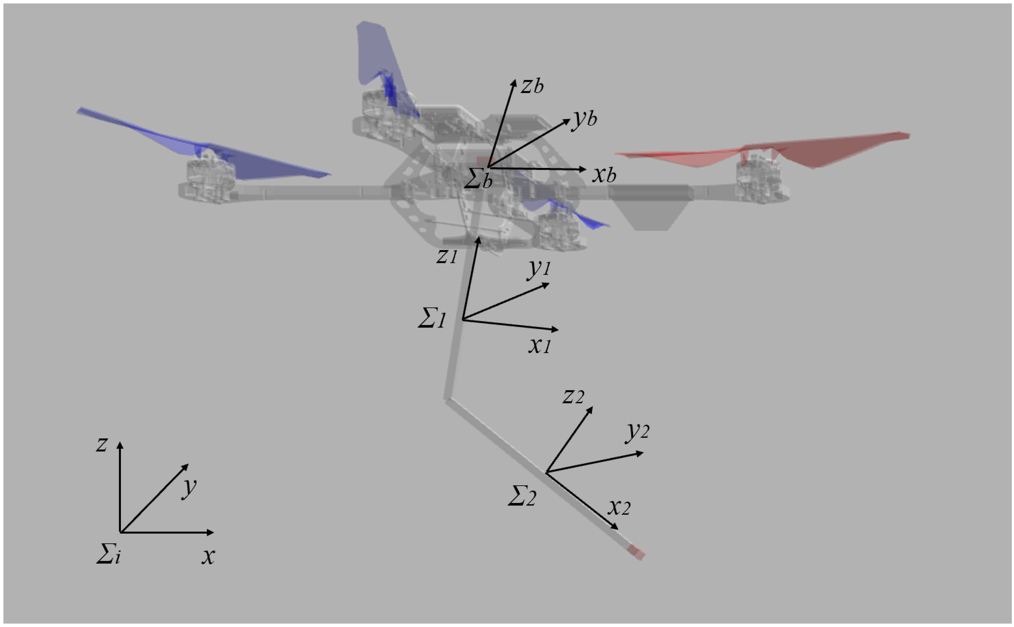
The aerial manipulation system consists of a quadrotor UAV with an attached 2-DOF planar manipulator. As shown in Figure 1, the following coordinate frame convention is adopted:

• Inertial frame Σ_I: This is the world-fixed reference frame;
• Body frame Σ_b: The quadrotor body-fixed frame with its origin at the center of mass and the Y-axis pointing into the paper (⊗);
• End-effector frame Σ_ee: This is located at the manipulator distal end.

Figure 1. System configuration with reference frames.

Figure 1. System configuration with reference frames.

The attached manipulator consists of two revolute joints; both joint axes are parallel to the quadrotor’s lateral axis (y_b-direction), enabling planar motion in the sagittal plane (x_b-z_b plane). It is considered that the position of the link’s center of mass and the end-effector are computed via forward kinematics expressed in the body-fixed frame, and these are obtained geometrically, as seen in Figure 1.

The complete system configuration is described by the following generalized coordinate vector:

$$\mathbf{q}={[x,y,z,\varphi ,\theta ,\psi ,{\theta }_1,{\theta }_2]}^T\in {\mathbb{R}}^8$$

(1)

where

• p = [x, y, z]^T represents the quadrotor center of mass position expressed in the inertial frame Σ_I;
• Φ = [ϕ, θ, ψ]^T denotes the Euler angles (roll, pitch, yaw) describing the orientation of the body-fixed frame Σ_b relative to the inertial frame Σ_I;
• η = [θ₁, θ₂]^T contains the manipulator joint angles defined in the body-fixed frame Σ_b.

The positive/negative sign convention results from the specific configuration, as presented next.

• Y-axis rotation joints: The Y-axis points into the paper (⊗);
• Positive angles are clockwise when viewed from the front and are consistent with the right-hand rule;
• Vertical reference: θ₁ = 0° corresponds to the arm hanging straight down;
• Motion direction: Positive angles rotate clockwise → movement toward negative (-)x_b direction.

2.1. Quadrotor Kinematics

The quadrotor kinematic equations are as follows:

$$\begin{array}{}\mathrm{(2)}& \hfill \dot{\mathbf{p}}& ={\mathbf{R}}_t{\dot{\mathbf{p}}}^b,\hfill \mathrm{(3)}& \hfill {\mathit{\omega }}_b& =\mathbf{Q}(\varphi ,\theta )\dot{\mathbf{\Phi }}\hfill \end{array}$$

where

$$\mathbf{Q}(\varphi ,\theta )=\left[\begin{array}{ccc}1& 0& -sin\theta \\ 0& cos\varphi & sin\varphi cos\theta \\ 0& -sin\varphi & cos\varphi cos\theta \end{array}\right]$$

(4)

R_t ∈ SO(3) is the rotation matrix from the body-fixed to the inertial frame. The body-fixed frame’s angular velocity ${\mathit{\omega }}_b\in {\mathbb{R}}^3$ is related to the Euler-rate vector $\dot{\mathbf{\Phi }}$. ${\dot{\mathbf{p}}}^b$ defines the linear velocity expressed in the body-fixed frame.

2.2. Manipulator Kinematics

Following the clockwise-positive convention with the Y-axis pointing inwards, the forward kinematics of the manipulator are derived using systematic kinematic chain analysis. Joint1 (θ₁) is attached at the quadrotor body-fixed frame origin Σ_b (quadrotor COM). Joint2 (θ₂) is located at the elbow between the two links. Link1 of length L₁ and Link2 of length L₂ are connected to Joint1 and Joint2, respectively.

Specifically, the center-of-mass position of Link1, given in (5), is obtained by extending halfway along Link1 from Joint1, as follows:

$${\mathbf{p}}_{1,COM}^b=\left[\begin{array}{c}-{\displaystyle \frac{L_1}{2}}sin({\theta }_1)\\ 0\\ -{\displaystyle \frac{L_1}{2}}cos({\theta }_1)\end{array}\right]$$

(5)

The center-of-mass position of Link2 is obtained by starting from the elbow (Joint2) position and adding a displacement of length L₂/2 along the direction of Link2, expressed in the quadrotor body-fixed frame.

The position of Joint2 is

$${\mathbf{p}}_{J2}^b=\left[\begin{array}{c}-L_{1}sin({\theta }_1)\\ 0\\ -L_{1}cos({\theta }_1)\end{array}\right]$$

(6)

The unit direction vector of Link2 is

$${\widehat{e}}_{L2}=\left[\begin{array}{c}-sin({\theta }_1+{\theta }_2)\\ 0\\ -cos({\theta }_1+{\theta }_2)\end{array}\right].$$

(7)

The center-of-mass position of Link2 is computed as [15]

$${\mathbf{p}}_{2,\mathrm{COM}}^b={\mathbf{p}}_{J2}^b+{\displaystyle \frac{L_2}{2}}{\widehat{e}}_{L2}$$

(8)

Substituting (6) and (7) into (8) leads to

$${\mathbf{p}}_{2,\mathrm{COM}}^b=\left[\begin{array}{c}-L_{1}sin({\theta }_1)-{\displaystyle \frac{L_2}{2}}sin({\theta }_1+{\theta }_2)\\ 0\\ -L_{1}cos({\theta }_1)-{\displaystyle \frac{L_2}{2}}cos({\theta }_1+{\theta }_2)\end{array}\right]$$

(9)

The position of the end-effector, given in (10), is defined as a point-mass located at the distal end of Link2 at a distance L₂ from Joint2 along the direction of the second link, as follows:

$${\mathbf{p}}_{ee}^b=\left[\begin{array}{c}-L_{1}sin({\theta }_1)-L_{2}sin({\theta }_1+{\theta }_2)\\ 0\\ -L_{1}cos({\theta }_1)-L_{2}cos({\theta }_1+{\theta }_2)\end{array}\right]$$

(10)

The linear velocities of the link centers of mass and end-effector, expressed in the quadrotor body-fixed frame, are obtained via the Jacobians of their position vectors with respect to the joint coordinates [15], expressed as follows:

$${\dot{\mathbf{p}}}_i^b(\mathit{\eta })={\mathbf{J}}_{p_i}(\mathit{\eta })\dot{\mathit{\eta }},\mathit{\eta }={[{\theta }_1,{\theta }_2]}^T,$$

(11)

where ${\mathbf{J}}_{p_i}(\mathit{\eta })\in {\mathbb{R}}^{3\times 2}$ is formed by obtaining the partial derivatives as

$${\mathbf{J}}_{p_i}(\mathit{\eta })=\left[\begin{array}{cc}{\displaystyle \frac{\partial {\mathbf{p}}_i^b}{\partial {\theta }_1}}& {\displaystyle \frac{\partial {\mathbf{p}}_i^b}{\partial {\theta }_2}}\end{array}\right]$$

(12)

The Jacobian terms are obtained by differentiating the corresponding position expressions for the link centers of mass and the end-effector given in (5), (9), and (10). Specifically, the Link1 velocity Jacobian terms are

$$\begin{array}{}\mathrm{(13)}& \hfill {\displaystyle \frac{\partial {\mathbf{p}}_{1,COM}^b}{\partial {\theta }_1}}& =\left[\begin{array}{c}-{\displaystyle \frac{L_1}{2}}cos({\theta }_1)\\ 0\\ {\displaystyle \frac{L_1}{2}}sin({\theta }_1)\end{array}\right]\hfill \mathrm{(14)}& \hfill {\displaystyle \frac{\partial {\mathbf{p}}_{1,COM}^b}{\partial {\theta }_2}}& =0_{3\times 1}\hfill \end{array}$$

The Link2 velocity Jacobian terms are

$$\begin{array}{}\mathrm{(15)}& \hfill {\displaystyle \frac{\partial {\mathbf{p}}_{2,COM}^b}{\partial {\theta }_1}}& =\left[\begin{array}{c}-L_{1}cos({\theta }_1)-{\displaystyle \frac{L_2}{2}}cos({\theta }_1+{\theta }_2)\\ 0\\ L_{1}sin({\theta }_1)+{\displaystyle \frac{L_2}{2}}sin({\theta }_1+{\theta }_2)\end{array}\right]\hfill \mathrm{(16)}& \hfill {\displaystyle \frac{\partial {\mathbf{p}}_{2,COM}^b}{\partial {\theta }_2}}& =\left[\begin{array}{c}-{\displaystyle \frac{L_2}{2}}cos({\theta }_1+{\theta }_2)\\ 0\\ {\displaystyle \frac{L_2}{2}}sin({\theta }_1+{\theta }_2)\end{array}\right]\hfill \end{array}$$

The end-effector velocity Jacobian terms are

$$\begin{array}{}\mathrm{(17)}& \hfill {\displaystyle \frac{\partial {\mathbf{p}}_{ee}^b}{\partial {\theta }_1}}& =\left[\begin{array}{c}-L_{1}cos({\theta }_1)-L_{2}cos({\theta }_1+{\theta }_2)\\ 0\\ L_{1}sin({\theta }_1)+L_{2}sin({\theta }_1+{\theta }_2)\end{array}\right]\hfill \mathrm{(18)}& \hfill {\displaystyle \frac{\partial {\mathbf{p}}_{ee}^b}{\partial {\theta }_2}}& =\left[\begin{array}{c}-L_{2}cos({\theta }_1+{\theta }_2)\\ 0\\ L_{2}sin({\theta }_1+{\theta }_2)\end{array}\right]\hfill \end{array}$$

2.3. Combined System Kinematics

World Frame Positions: The position of each term in the world frame is given by the following general transformation [15]:

$${\mathbf{p}}_{i,COM}^W=\mathbf{p}+{\mathbf{R}}_t{\mathbf{p}}_{i,COM}^b$$

(19)

The Link1 COM expressed in the world frame is

$${\mathbf{p}}_{1,COM}^W=\left[\begin{array}{c}x\\ y\\ z\end{array}\right]+{\mathbf{R}}_t\left[\begin{array}{c}-{\displaystyle \frac{L_1}{2}}sin({\theta }_1)\\ 0\\ -{\displaystyle \frac{L_1}{2}}cos({\theta }_1)\end{array}\right]$$

(20)

The Link2 COM expressed in the world frame is

$${\mathbf{p}}_{2,COM}^W=\left[\begin{array}{c}x\\ y\\ z\end{array}\right]+{\mathbf{R}}_t\left[\begin{array}{c}-L_{1}sin({\theta }_1)-{\displaystyle \frac{L_2}{2}}sin({\theta }_1+{\theta }_2)\\ 0\\ -L_{1}cos({\theta }_1)-{\displaystyle \frac{L_2}{2}}cos({\theta }_1+{\theta }_2)\end{array}\right]$$

(21)

The end-effector COM expressed in the world frame is

$${\mathbf{p}}_{ee}^W=\left[\begin{array}{c}x\\ y\\ z\end{array}\right]+{\mathbf{R}}_t\left[\begin{array}{c}-L_{1}sin({\theta }_1)-L_{2}sin({\theta }_1+{\theta }_2)\\ 0\\ -L_{1}cos({\theta }_1)-L_{2}cos({\theta }_1+{\theta }_2)\end{array}\right]$$

(22)

Velocity Relationships: The velocity of each term expressed in the world frame is obtained by taking the following time derivative [15]:

$${\dot{\mathbf{p}}}_{i,COM}^W=\dot{\mathbf{p}}+{\dot{\mathbf{R}}}_t{\mathbf{p}}_{i,COM}^b+{\mathbf{R}}_t{\dot{\mathbf{p}}}_{i,COM}^b$$

(23)

Using the rotation matrix ${\dot{\mathbf{R}}}_t={\mathbf{R}}_{t}S({\mathit{\omega }}_b)$, where ω_b denotes the angular velocity expressed in the body-fixed frame, the following is obtained:

$${\dot{\mathbf{p}}}_{i,COM}^W=\dot{\mathbf{p}}+{\mathbf{R}}_t({\mathit{\omega }}_b \times {\mathbf{p}}_{i,COM}^b+{\dot{\mathbf{p}}}_{i,COM}^b)$$

(24)

Unified System Velocity: The complete system velocity relationships can be expressed in matrix form as [15]

$${\dot{\mathbf{p}}}_{i,COM}^W={\mathbf{J}}_{i,v}\dot{\mathbf{q}}$$

(25)

where ${\mathbf{J}}_{i,v}\in {\mathbb{R}}^{3\times 8}$ is the velocity Jacobian matrix for term i, mapping the system velocity $\dot{\mathbf{q}}$ (generalized velocity vector) to the component’s linear velocity in the world frame.

The velocity Jacobian for component i may be written as

$${\mathbf{J}}_{i,v}=\left[\begin{array}{cccc}{\mathbb{I}}_3& -{\mathbf{R}}_{t}S({\mathbf{p}}_{i,COM}^b)\mathbf{Q}& {\mathbf{R}}_t{\displaystyle \frac{\partial {\mathbf{p}}_{i,COM}^b}{\partial {\theta }_1}}& {\mathbf{R}}_t{\displaystyle \frac{\partial {\mathbf{p}}_{i,COM}^b}{\partial {\theta }_2}}\end{array}\right],$$

(26)

where S(·) denotes the skew-symmetric matrix associated with the cross product.

3. Dynamic Model

The E-L formulation is followed. The Lagrangian is derived as

$$\mathcal{L}(\mathbf{q},\dot{\mathbf{q}})=T(\mathbf{q},\dot{\mathbf{q}})-\mathcal{U}(\mathbf{q})$$

(27)

where T is the total kinetic energy and $\mathcal{U}$ is the total potential energy of the combined system. All manipulator kinematics are expressed in the quadrotor body-fixed frame Σ_b and mapped to the inertial frame via R_t. Angular velocities are expressed in the body-fixed frame.

3.1. Kinetic Energy Analysis

Following [15], the total kinetic energy is

$$T=T_{quad}+T_{link1}+T_{link2}+T_{ee}$$

(28)

The quadrotor kinetic energy is

$$T_{quad}={\displaystyle \frac{1}{2}}{m}_b{\dot{\mathbf{p}}}^T\dot{\mathbf{p}}+{\displaystyle \frac{1}{2}}{\mathit{\omega }}_b^T{\mathbf{I}}_b{\mathit{\omega }}_b$$

(29)

where m_b is the quadrotor mass, $\dot{\mathbf{p}}={[\dot{x},\dot{y},\dot{z}]}^T$ is the quadrotor linear velocity, ω_b is the quadrotor angular velocity in the body-fixed frame, and I_b = diag(I_xx, I_yy, I_zz) is the quadrotor inertia tensor. Using the kinematic relationship of the quadrotor (3), the following is obtained:

$${\mathit{\omega }}_b=\mathbf{Q}\dot{\mathbf{\Phi }}=\mathbf{Q}{[\dot{\varphi },\dot{\theta },\dot{\psi }]}^T$$

(30)

The Link1 kinetic energy is

$$T_{link1}={\displaystyle \frac{1}{2}}{m}_1{\dot{\mathbf{p}}}_{1,COM}^{W^T}{\dot{\mathbf{p}}}_{1,COM}^W+{\displaystyle \frac{1}{2}}{\mathit{\omega }}_1^T{\mathbf{I}}_1{\mathit{\omega }}_1$$

(31)

Using the expression (24) from the kinematic analysis, the Link1 COM velocity in the world frame is

$${\dot{\mathbf{p}}}_{1,COM}^W=\dot{\mathbf{p}}+{\mathbf{R}}_t({\mathit{\omega }}_b\times {\mathbf{p}}_{1,COM}^b+{\dot{\mathbf{p}}}_{1,COM}^b)$$

(32)

Using the Link1 velocity Jacobian (13), the following is obtained:

$${\dot{\mathbf{p}}}_{1,COM}^b={\displaystyle \frac{\partial {\mathbf{p}}_{1,COM}^b}{\partial {\theta }_1}}{\dot{\theta }}_1=\left[\begin{array}{c}-{\displaystyle \frac{L_1}{2}}cos({\theta }_1)\\ 0\\ {\displaystyle \frac{L_1}{2}}sin({\theta }_1)\end{array}\right]{\dot{\theta }}_1$$

(33)

Likewise, the Link1 angular velocity consists of the quadrotor rotation plus the joint rotation, as follows:

$${\mathit{\omega }}_1={\mathit{\omega }}_b+{\dot{\theta }}_1{\mathbf{e}}_y$$

(34)

where e_y = [0, 1, 0]^T is the unit vector of the joint axis y_b, expressed in Σ_b. Thus, ω₁ and ω₂ are expressed in Σ_b.

The Link2 kinetic energy is

$$T_{link2}={\displaystyle \frac{1}{2}}{m}_2{\dot{\mathbf{p}}}_{2,COM}^{W^T}{\dot{\mathbf{p}}}_{2,COM}^W+{\displaystyle \frac{1}{2}}{\mathit{\omega }}_2^T{\mathbf{I}}_2{\mathit{\omega }}_2$$

(35)

Using the expression (24) from the kinematic analysis, the Link2 COM velocity in the world frame is

$${\dot{\mathbf{p}}}_{2,COM}^W=\dot{\mathbf{p}}+{\mathbf{R}}_t({\mathit{\omega }}_b\times {\mathbf{p}}_{2,COM}^b+{\dot{\mathbf{p}}}_{2,COM}^b)$$

(36)

Using the Link2 velocity Jacobians (15) and (16), the following is obtained:

$${\dot{\mathbf{p}}}_{2,COM}^b={\displaystyle \frac{\partial {\mathbf{p}}_{2,COM}^b}{\partial {\theta }_1}}{\dot{\theta }}_1+{\displaystyle \frac{\partial {\mathbf{p}}_{2,COM}^b}{\partial {\theta }_2}}{\dot{\theta }}_2$$

(37)

The Link2 angular velocity includes both joint rotations, as follows:

$${\mathit{\omega }}_2={\mathit{\omega }}_b+{\dot{\theta }}_1{\mathbf{e}}_y+{\dot{\theta }}_2{\mathbf{e}}_y$$

(38)

The manipulator link rotational kinetic energy is computed about the body-fixed y_b-axis. Since the manipulator is planar and both joints rotate about the same axis, each link’s angular velocity is parallel to y_b. Consequently, only the principal moment of inertia about this axis, I_yy, contributes to the link rotational kinetic energy.

For the point mass end-effector, the following is obtained:

$$T_{ee}={\displaystyle \frac{1}{2}}{m}_{ee}{\dot{\mathbf{p}}}_{ee}^{W^T}{\dot{\mathbf{p}}}_{ee}^W$$

(39)

where

$${\dot{\mathbf{p}}}_{ee}^W=\dot{\mathbf{p}}+{\mathbf{R}}_t({\mathit{\omega }}_b\times {\mathbf{p}}_{ee}^b+{\dot{\mathbf{p}}}_{ee}^b)$$

(40)

3.2. Potential Energy Analysis

The total potential energy consists of the gravitational potential energy of all masses, as follows [15]:

$$\mathcal{U}={\mathcal{U}}_{quad}+{\mathcal{U}}_{link1}+{\mathcal{U}}_{link2}+{\mathcal{U}}_{ee}$$

(41)

Gravitational Potential Energy: The quadrotor potential energy is

$${\mathcal{U}}_{quad}=m_{b}g{\mathbf{e}}_z^T\mathbf{p}$$

(42)

Each link and end-effector potential energy is expressed as [16]

$${\mathcal{U}}_{linki}=m_{i}g{\mathbf{e}}_z^T{\mathbf{p}}_{i,COM}^W$$

(43)

where e_z = [0, 0, 1]^T extracts the Z-component (height).

Substituting the world frame positions from the kinematic analysis, namely (20), (21), and (22), into (43), the following is obtained:

$${\mathcal{U}}_{link1}=m_{1}g\left(z+{\mathbf{e}}_z^T{\mathbf{R}}_t\left[\begin{array}{c}-{\displaystyle \frac{L_1}{2}}sin({\theta }_1)\\ 0\\ -{\displaystyle \frac{L_1}{2}}cos({\theta }_1)\end{array}\right]\right)$$

(44)

$${\mathcal{U}}_{link2}=m_{2}g\left(z+{\mathbf{e}}_z^T{\mathbf{R}}_t\left[\begin{array}{c}-L_{1}sin({\theta }_1)-{\displaystyle \frac{L_2}{2}}sin({\theta }_1+{\theta }_2)\\ 0\\ -L_{1}cos({\theta }_1)-{\displaystyle \frac{L_2}{2}}cos({\theta }_1+{\theta }_2)\end{array}\right]\right)$$

(45)

$${\mathcal{U}}_{ee}=m_{ee}g\left(z+{\mathbf{e}}_z^T{\mathbf{R}}_t\left[\begin{array}{c}-L_{1}sin({\theta }_1)-L_{2}sin({\theta }_1+{\theta }_2)\\ 0\\ -L_{1}cos({\theta }_1)-L_{2}cos({\theta }_1+{\theta }_2)\end{array}\right]\right)$$

(46)

3.3. Lagrangian Formulation

The complete system dynamics are described by [15]

$${\displaystyle \frac{d}{dt}}\left({\displaystyle \frac{\partial \mathcal{L}}{\partial \dot{\mathbf{q}}}}\right)-{\displaystyle \frac{\partial \mathcal{L}}{\partial \mathbf{q}}}=\mathit{\tau }$$

(47)

where $\mathcal{L}=T-\mathcal{U}$ is the Lagrangian, with T representing total kinetic energy and $\mathcal{U}$, total potential energy.

Substituting the calculated kinetic and potential energies, the complete Lagrangian is

$$\begin{array}{}& \hfill \mathcal{L}& =T_{quad}+T_{link1}+T_{link2}+T_{ee}\hfill \mathrm{(48)}& & -{\mathcal{U}}_{quad}-{\mathcal{U}}_{link1}-{\mathcal{U}}_{link2}-{\mathcal{U}}_{ee}\hfill \end{array}$$

This leads to the following standard robotic equation of motion [17]:

$$\mathbf{M}(\mathbf{q})\ddot{\mathbf{q}}+\mathbf{C}(\mathbf{q},\dot{\mathbf{q}})\dot{\mathbf{q}}+\mathbf{G}(\mathbf{q})=\mathit{\tau }$$

(49)

where M(q) is the symmetric positive-definite mass matrix, $\mathbf{C}(\mathbf{q},\dot{\mathbf{q}})$ gives Coriolis and centrifugal terms, and G(q) represents gravitational effects.

3.4. Kinetic Energy Matrix Derivation

The total kinetic energy of the system can be written in the quadratic form [16]

$$T={\displaystyle \frac{1}{2}}{\dot{\mathbf{q}}}^T\mathbf{M}(\mathbf{q})\dot{\mathbf{q}}$$

(50)

where $\mathbf{M}(\mathbf{q})\in {\mathbb{R}}^{8\times 8}$ is the symmetric positive-definite mass matrix.

Due to the coupling between translational, rotational, and manipulator dynamics, the mass matrix has the block structure of a floating-based system, as follows [18]:

$$\mathbf{M}(\mathbf{q})=\left[\begin{array}{cc}{\mathbf{M}}_{qq}& {\mathbf{M}}_{q\eta }\\ {\mathbf{M}}_{\eta q}& {\mathbf{M}}_{\eta \eta }\end{array}\right]$$

(51)

where ${\mathbf{M}}_{qq}\in {\mathbb{R}}^{6\times 6}$ represents quadrotor–quadrotor inertial coupling, ${\mathbf{M}}_{q\eta }\in {\mathbb{R}}^{6\times 2}$ holds the quadrotor–manipulator coupling, ${\mathbf{M}}_{\eta q}={\mathbf{M}}_{q\eta }^T\in {\mathbb{R}}^{2\times 6}$ represents manipulator–quadrotor coupling, and ${\mathbf{M}}_{\eta \eta }\in {\mathbb{R}}^{2\times 2}$ is the manipulator–manipulator coupling.

Quadrotor–Quadrotor Block: The quadrotor block M_qq is obtained by collecting the terms of the kinetic energy associated with the quadrotor generalized velocities ${[\dot{x},\dot{y},\dot{z},\dot{\varphi },\dot{\theta },\dot{\psi }]}^T$. Using the component velocity relationship in (24), the kinetic energy expansion yields translational, rotational, and translation–rotation coupling terms. The ${\mathbf{M}}_{qq}\in {\mathbb{R}}^{6\times 6}$ block has the form

$${\mathbf{M}}_{qq}=\left[\begin{array}{cc}{\mathbf{M}}_{tt}& {\mathbf{M}}_{tr}\\ {\mathbf{M}}_{rt}& {\mathbf{M}}_{rr}\end{array}\right]$$

(52)

where M_tt is the translational inertia block, M_rr is the rotational inertia block, and M_tr captures translation–rotation coupling with ${\mathbf{M}}_{rt}={\mathbf{M}}_{tr}^T$.

The translational inertia block M_tt contains kinetic energy terms associated with the translational velocity ${\dot{\mathbf{p}}}_b={[\dot{x},\dot{y},\dot{z}]}^T$. From the velocity expression in (24), the translational velocity ${\dot{\mathbf{p}}}_b$ appears identically in the kinetic energy of the quadrotor, both links, and the end-effector. As a result, each mass contributes additively to the translational inertia. Therefore, the translational block is given by

$${\mathbf{M}}_{tt}=(m_b+m_1+m_2+m_{ee}){\mathbb{I}}_{3\times 3}$$

(53)

The translation–rotation coupling block arises from the rotational term ${\mathbf{R}}_t({\mathit{\omega }}_b\times {\mathbf{p}}_{i,COM}^b)$ in the velocity expression (24). This term represents the linear velocity induced at each link and the end-effector center of mass due to the rotational motion of the quadrotor base about an offset position ${\mathbf{p}}_{i,COM}^b$. When expanding the kinetic energy, cross terms between the translational velocity ${\dot{\mathbf{p}}}_b$ and the rotation-induced velocity ${\mathit{\omega }}_b\times {\mathbf{p}}_{i,COM}^b$ produce translation–rotation coupling terms in the mass matrix. Using the cross product identity a × b = − S(b)a [15] and the relation ${\mathit{\omega }}_b=\mathbf{Q}\dot{\mathbf{\Phi }}$, the translation–rotation block becomes

$$\begin{array}{}\mathrm{(54)}& \hfill {\mathbf{M}}_{tr}& =-(m_{1}S({\mathbf{R}}_t{\mathbf{p}}_{1,COM}^b)+m_{2}S({\mathbf{R}}_t{\mathbf{p}}_{2,COM}^b)\hfill \mathrm{(55)}& & +m_{ee}S({\mathbf{R}}_t{\mathbf{p}}_{ee}^b)){\mathbf{R}}_t\mathbf{Q}\hfill \end{array}$$

where the skew-symmetric operator is defined as

$$S(a)=\left[\begin{array}{ccc}0& -a_z& a_y\\ a_z& 0& -a_x\\ -a_y& a_x& 0\end{array}\right]$$

(56)

By symmetry of the inertia matrix, ${\mathbf{M}}_{rt}={\mathbf{M}}_{tr}^T$.

The rotational inertia block M_rr is obtained by expressing the rotational kinetic energy of the quadrotor, links, and end-effector in terms of the Euler-rate vector $\dot{\mathbf{\Phi }}$. Using the relation ${\mathit{\omega }}_b=\mathbf{Q}\dot{\mathbf{\Phi }}$, the inertia terms can be grouped to form the rotational block of the mass matrix, as follows:

$$\begin{array}{cc}\hfill {\mathbf{M}}_{rr}& ={\mathbf{Q}}^T({\mathbf{I}}_b+I_{1,yy}{\mathbf{e}}_y{\mathbf{e}}_y^T+I_{2,yy}{\mathbf{e}}_y{\mathbf{e}}_y^T\hfill \\ & +m_{1}S{({\mathbf{p}}_{1,COM}^b)}^{T}S({\mathbf{p}}_{1,COM}^b)\hfill \\ & +m_{2}S{({\mathbf{p}}_{2,COM}^b)}^{T}S({\mathbf{p}}_{2,COM}^b)\hfill \\ & +m_{ee}S{({\mathbf{p}}_{ee}^b)}^{T}S({\mathbf{p}}_{ee}^b))\mathbf{Q}\hfill \end{array}$$

(57)

The first term represents the rotational inertia of the quadrotor body. The second and third terms account for the planar rotational inertia of the two manipulator links about the y_b axis. The remaining terms arise from the parallel-axis effect due to the offset of each mass from the quadrotor center, captured using the skew-symmetric formulation [15].

Quadrotor–Manipulator Coupling Block: The quadrotor–manipulator block ${\mathbf{M}}_{q\eta }\in {\mathbb{R}}^{6\times 2}$ has the following form:

$${\mathbf{M}}_{q\eta }=\left[\begin{array}{c}{\mathbf{M}}_{t\eta }\\ {\mathbf{M}}_{r\eta }\end{array}\right]$$

(58)

where ${\mathbf{M}}_{t\eta }\in {\mathbb{R}}^{3\times 2}$ represents the translational coupling between the quadrotor linear motion and manipulator joint velocities, and ${\mathbf{M}}_{r\eta }\in {\mathbb{R}}^{3\times 2}$ represents the rotational coupling between quadrotor attitude dynamics and joint motion.

The translation–joint coupling block M_tη emerges from the cross terms between the quadrotor translational velocity ${\dot{\mathbf{p}}}_b$ and the joint velocities of the link and end-effector centers of mass. Specifically, when expanding the kinetic energy $T_i={\displaystyle \frac{1}{2}}{m}_i|{\dot{\mathbf{p}}}_b$$+{\mathbf{R}}_t({\mathit{\omega }}_b\times {\mathbf{p}}_i^b+{\dot{\mathbf{p}}}_i^b){|}^2$, the cross term ($2{\dot{\mathbf{p}}}_b·{\mathbf{R}}_t{\dot{\mathbf{p}}}_i^b$) creates coupling between the quadrotor translation and joint velocities. Taking the second derivatives ${\displaystyle \frac{{\partial }^{2}T}{\partial {\dot{\mathbf{p}}}_b\partial {\dot{\theta }}_j}}$ leads to

$$\begin{array}{}& \hfill {\mathbf{M}}_{t\eta }& =m_1{\mathbf{R}}_t\left[\begin{array}{cc}{\displaystyle \frac{\partial {\mathbf{p}}_{1,COM}^b}{\partial {\theta }_1}}& 0\end{array}\right]+m_2{\mathbf{R}}_t\left[\begin{array}{cc}{\displaystyle \frac{\partial {\mathbf{p}}_{2,COM}^b}{\partial {\theta }_1}}& {\displaystyle \frac{\partial {\mathbf{p}}_{2,COM}^b}{\partial {\theta }_2}}\end{array}\right]\hfill \mathrm{(59)}& & +m_{ee}{\mathbf{R}}_t\left[\begin{array}{cc}{\displaystyle \frac{\partial {\mathbf{p}}_{ee}^b}{\partial {\theta }_1}}& {\displaystyle \frac{\partial {\mathbf{p}}_{ee}^b}{\partial {\theta }_2}}\end{array}\right]\hfill \end{array}$$

The rotation–joint coupling block M_rη arises from two distinct sources in the kinetic energy expansion. The first source emerges from the cross term $2({\mathit{\omega }}_b\times {\mathbf{p}}_i^b)·{\dot{\mathbf{p}}}_i^b$, where the quadrotor angular velocities ${\mathit{\omega }}_b=\mathbf{Q}\dot{\mathbf{\Phi }}$ interact with joint-induced motions of displaced masses. Taking the mixed derivatives $\frac{{\partial }^{2}T}{\partial \dot{\mathbf{\Phi }}\partial {\dot{\theta }}_j}$ yields the skew-symmetric coupling terms. The second source comes from the rotational inertia coupling between the quadrotor angular motion and joint angular velocities through the link inertias I_j,yy. This results in

$$\begin{array}{}& \hfill {\mathbf{M}}_{r\eta }& =m_1{\mathbf{Q}}^{T}S({\mathbf{p}}_{1,COM}^b)\left[\begin{array}{cc}{\displaystyle \frac{\partial {\mathbf{p}}_{1,COM}^b}{\partial {\theta }_1}}& 0\end{array}\right]\hfill & & +m_2{\mathbf{Q}}^{T}S({\mathbf{p}}_{2,COM}^b)\left[\begin{array}{cc}{\displaystyle \frac{\partial {\mathbf{p}}_{2,COM}^b}{\partial {\theta }_1}}& {\displaystyle \frac{\partial {\mathbf{p}}_{2,COM}^b}{\partial {\theta }_2}}\end{array}\right]\hfill & & +m_{ee}{\mathbf{Q}}^{T}S({\mathbf{p}}_{ee}^b)\left[\begin{array}{cc}{\displaystyle \frac{\partial {\mathbf{p}}_{ee}^b}{\partial {\theta }_1}}& {\displaystyle \frac{\partial {\mathbf{p}}_{ee}^b}{\partial {\theta }_2}}\end{array}\right]\hfill \mathrm{(60)}& & +I_{1,yy}{\mathbf{Q}}^T{\mathbf{e}}_y\left[\begin{array}{cc}1& 0\end{array}\right]+I_{2,yy}{\mathbf{Q}}^T{\mathbf{e}}_y\left[\begin{array}{cc}1& 1\end{array}\right]\hfill \end{array}$$

Manipulator–Manipulator Block: The manipulator–manipulator block emerges from the joint motion terms in the kinetic energy expansion. From the velocity relationship (24), the joint motion contribution $({\mathbf{R}}_t{\dot{\mathbf{p}}}_i^b)$ creates kinetic energy terms of the form ${\displaystyle \frac{1}{2}}{m}_i{\left|{\mathbf{R}}_t{\dot{\mathbf{p}}}_i^b\right|}^2$. Expanding the joint velocities ${\dot{\mathbf{p}}}_i^b={\displaystyle \frac{\partial {\mathbf{p}}_i^b}{\partial {\theta }_1}}{\dot{\theta }}_1+{\displaystyle \frac{\partial {\mathbf{p}}_i^b}{\partial {\theta }_2}}{\dot{\theta }}_2$ and taking the second derivatives ${\displaystyle \frac{{\partial }^{2}T}{\partial {\dot{\theta }}_i\partial {\dot{\theta }}_j}}$, the mass matrix elements become the products of velocity Jacobians. Additionally, the rotational kinetic energy of each link about its joint axis contributes the inertia terms I_j,yy.

The manipulator–manipulator block ${\mathbf{M}}_{\eta \eta }\in {\mathbb{R}}^{2\times 2}$ has the following form:

$$\begin{array}{cc}\hfill {\mathbf{M}}_{\eta \eta }& =m_1{\mathbf{J}}_1^T{\mathbf{J}}_1+m_2{\mathbf{J}}_2^T{\mathbf{J}}_2+m_{ee}{\mathbf{J}}_{ee}^T{\mathbf{J}}_{ee}\hfill \\ & +\left[\begin{array}{cc}{I}_{1,yy}+I_{2,yy}& I_{2,yy}\\ I_{2,yy}& I_{2,yy}\end{array}\right].\hfill \end{array}$$

(61)

$$\begin{array}{cc}\hfill {\mathbf{J}}_1& =\left[\begin{array}{cc}{\displaystyle \frac{\partial {\mathbf{p}}_{1,COM}^b}{\partial {\theta }_1}}& 0\end{array}\right],{\mathbf{J}}_2=\left[\begin{array}{cc}{\displaystyle \frac{\partial {\mathbf{p}}_{2,COM}^b}{\partial {\theta }_1}}& {\displaystyle \frac{\partial {\mathbf{p}}_{2,COM}^b}{\partial {\theta }_2}}\end{array}\right],\hfill \\ \hfill {\mathbf{J}}_{ee}& =\left[\begin{array}{cc}{\displaystyle \frac{\partial {\mathbf{p}}_{ee}^b}{\partial {\theta }_1}}& {\displaystyle \frac{\partial {\mathbf{p}}_{ee}^b}{\partial {\theta }_2}}\end{array}\right].\hfill \end{array}$$

(62)

Computing the dot products analytically results in

$$\begin{array}{}& \hfill M_{\eta \eta ,11}& ={\displaystyle \frac{m_1{L}_1^2}{4}}+m_2{L}_1^2+{\displaystyle \frac{m_2{L}_2^2}{4}}+m_2{L}_1{L}_{2}cos({\theta }_2)\hfill \mathrm{(63)}& & +m_{ee}{L}_1^2+m_{ee}{L}_2^2+2m_{ee}{L}_1{L}_{2}cos({\theta }_2)\hfill \mathrm{(64)}& & +I_{1,yy}+I_{2,yy}\hfill \end{array}$$

$$\begin{array}{}& \hfill M_{\eta \eta ,12}=M_{\eta \eta ,21}& ={\displaystyle \frac{m_2{L}_2^2}{4}}+{\displaystyle \frac{m_2{L}_1{L}_2}{2}}cos({\theta }_2)\hfill \mathrm{(65)}& & +m_{ee}{L}_2^2+m_{ee}{L}_1{L}_{2}cos({\theta }_2)\hfill \mathrm{(66)}& & +I_{2,yy}\hfill \end{array}$$

$$M_{\eta \eta ,22}={\displaystyle \frac{m_2{L}_2^2}{4}}+m_{ee}{L}_2^2+I_{2,yy}$$

(67)

3.5. Coriolis Matrix Computation

The Coriolis matrix $\mathbf{C}(\mathbf{q},\dot{\mathbf{q}})\in {\mathbb{R}}^{8\times 8}$ is computed using Christoffel symbols as follows [17]:

$$C_{ij}=\sum _{k=1}^8{\mathrm{\Gamma }}_{ij}^k{\dot{\mathbf{q}}}_k$$

(68)

where ${\dot{\mathbf{q}}}_k$ denotes the velocity associated with the k-th generalized coordinate.

Christoffel symbols are defined as

$${\mathrm{\Gamma }}_{ij}^k={\displaystyle \frac{1}{2}}\left({\displaystyle \frac{\partial M_{ij}}{\partial {\mathbf{q}}_k}}+{\displaystyle \frac{\partial M_{ik}}{\partial {\mathbf{q}}_j}}-{\displaystyle \frac{\partial M_{kj}}{\partial {\mathbf{q}}_i}}\right)$$

(69)

where M_ij indicates the (i, j)-th element of the mass matrix M(q) [11].

Coriolis Matrix Structure: Due to the coupled aerial–manipulator system, the Coriolis matrix contains velocity-dependent terms arising from quadrotor motion, manipulator motion, and their interactions. The Coriolis matrix can be written as

$$\mathbf{C}(\mathbf{q},\dot{\mathbf{q}})=\left[\begin{array}{cc}{\mathbf{C}}_{qq}& {\mathbf{C}}_{q\eta }\\ {\mathbf{C}}_{\eta q}& {\mathbf{C}}_{\eta \eta }\end{array}\right]$$

(70)

where ${\mathbf{C}}_{qq}\in {\mathbb{R}}^{6\times 6}$ contains velocity-dependent terms acting on the quadrotor base due to base motion, ${\mathbf{C}}_{q\eta }\in {\mathbb{R}}^{6\times 2}$ represents coupling effects induced by manipulator joint velocities on the quadrotor dynamics, ${\mathbf{C}}_{\eta q}\in {\mathbb{R}}^{2\times 6}$ captures velocity-dependent torques on the manipulator joints caused by quadrotor motion, and ${\mathbf{C}}_{\eta \eta }\in {\mathbb{R}}^{2\times 2}$ corresponds to the Coriolis and centrifugal effects of the manipulator subsystem.

The C_ηη coupling terms are substituted with partial derivatives from the mass matrix in Appendix C. The remaining Coriolis terms arise from the configuration dependence of the coupled mass matrix blocks. In particular, attitude-dependent coupling terms in both C_qη and C_ηq originate from ∂M_qη/∂Φ, derivatives of the base inertia block M_qq with respect to Φ and η, and contribute to C_qq, and since M_ηη is independent of θ₁ and depends only on θ₂, the C_ηη block is derived from the partial derivatives of M_ηη [15]. The complete partial derivative expressions for all blocks are provided in Appendix C.

3.6. Gravity Vector Derivation

The gravity vector $\mathbf{G}(\mathbf{q})\in {\mathbb{R}}^8$ is obtained from partial derivatives of the following expression [15]:

$$G_i={\displaystyle \frac{\partial \mathcal{U}}{\partial {\mathbf{q}}_i}}$$

(71)

where q_i denotes the i-th generalized coordinate of the system state vector q.

Although the full gravity vector of the coupled system is derived via the E-L formulation for completeness, in the implementation, the quadrotor weight is compensated by the RotorS geometric position controller [14]. In particular, gravity appears through the term $-g{\mathbf{e}}_3$ (where ${\mathbf{e}}_3={[001]}^T$ denotes the unit vector along the world-frame z-axis) in the commanded translational acceleration and is converted to thrust by projecting the commanded force onto the body-fixed z-axis. To avoid double counting, the base gravity terms are therefore not injected through G(q) in the computed torque law. The system operates near hover, and the manipulator gravity depends primarily on the joint configuration; hence, for the planar arm, the joint gravity terms are evaluated using a reduced model under the small-roll-and-pitch assumption [11].

Quadrotor Gravity Terms: The quadrotor gravity terms for translation are

$${\displaystyle \frac{\partial \mathcal{U}}{\partial x}}=0,{\displaystyle \frac{\partial \mathcal{U}}{\partial y}}=0,{\displaystyle \frac{\partial \mathcal{U}}{\partial z}}=(m_b+m_1+m_2+m_{ee})g$$

(72)

The gravity terms associated with quadrotor attitude are retained in symbolic form for simplicity as follows:

$${\displaystyle \frac{\partial \mathcal{U}}{\partial \varphi }}=g\sum _{i=1,2,ee}{m}_i{\displaystyle \frac{\partial }{\partial \varphi }}\left({\mathbf{e}}_z^T{\mathbf{R}}_t{\mathbf{p}}_{i,COM}^b\right)$$

(73)

$${\displaystyle \frac{\partial \mathcal{U}}{\partial \theta }}=g\sum _{i=1,2,ee}{m}_i{\displaystyle \frac{\partial }{\partial \theta }}\left({\mathbf{e}}_z^T{\mathbf{R}}_t{\mathbf{p}}_{i,COM}^b\right)$$

(74)

$${\displaystyle \frac{\partial \mathcal{U}}{\partial \psi }}=g\sum _{i=1,2,ee}{m}_i{\displaystyle \frac{\partial }{\partial \psi }}\left({\mathbf{e}}_z^T{\mathbf{R}}_t{\mathbf{p}}_{i,COM}^b\right)$$

(75)

Joint Gravity Terms: Using the general form (75), the joint gravity terms for each joint lead to

$$\begin{array}{cc}\hfill G_{{\theta }_1}& ={\displaystyle \frac{\partial \mathcal{U}}{\partial {\theta }_1}}=g[m_1{\displaystyle \frac{\partial }{\partial {\theta }_1}}\left({\mathbf{e}}_z^T{\mathbf{R}}_t{\mathbf{p}}_{1,\mathrm{COM}}^b\right)\hfill \\ & +m_2{\displaystyle \frac{\partial }{\partial {\theta }_1}}\left({\mathbf{e}}_z^T{\mathbf{R}}_t{\mathbf{p}}_{2,\mathrm{COM}}^b\right)+m_{ee}{\displaystyle \frac{\partial }{\partial {\theta }_1}}\left({\mathbf{e}}_z^T{\mathbf{R}}_t{\mathbf{p}}_{ee}^b\right)]\hfill \end{array}$$

(76)

$$\begin{array}{cc}\hfill G_{{\theta }_2}& ={\displaystyle \frac{\partial \mathcal{U}}{\partial {\theta }_2}}=g[m_2{\displaystyle \frac{\partial }{\partial {\theta }_2}}\left({\mathbf{e}}_z^T{\mathbf{R}}_t{\mathbf{p}}_{2,\mathrm{COM}}^b\right)\hfill \\ & +m_{ee}{\displaystyle \frac{\partial }{\partial {\theta }_2}}\left({\mathbf{e}}_z^T{\mathbf{R}}_t{\mathbf{p}}_{ee}^b\right)]\hfill \end{array}$$

(77)

Under the small-roll-and-pitch-angle assumption, where the quadrotor maintains approximately level flight [11] (${\mathbf{R}}_t\approx \mathbb{I}$), the joint gravity terms reduce to

$$\begin{array}{cc}\hfill G_{{\theta }_1}=& g[{\displaystyle \frac{m_1{L}_1}{2}}sin({\theta }_1)+m_2{L}_{1}sin({\theta }_1)\hfill \\ & +{\displaystyle \frac{m_2{L}_2}{2}}sin({\theta }_1+{\theta }_2)+m_{ee}{L}_{1}sin({\theta }_1)\hfill \\ & +m_{ee}{L}_{2}sin({\theta }_1+{\theta }_2)]\hfill \end{array}$$

(78)

$$G_{{\theta }_2}=g\left[{\displaystyle \frac{m_2{L}_2}{2}}sin({\theta }_1+{\theta }_2)+m_{ee}{L}_{2}sin({\theta }_1+{\theta }_2)\right]$$

(79)

4. Control Design

4.1. Control Architecture Overview

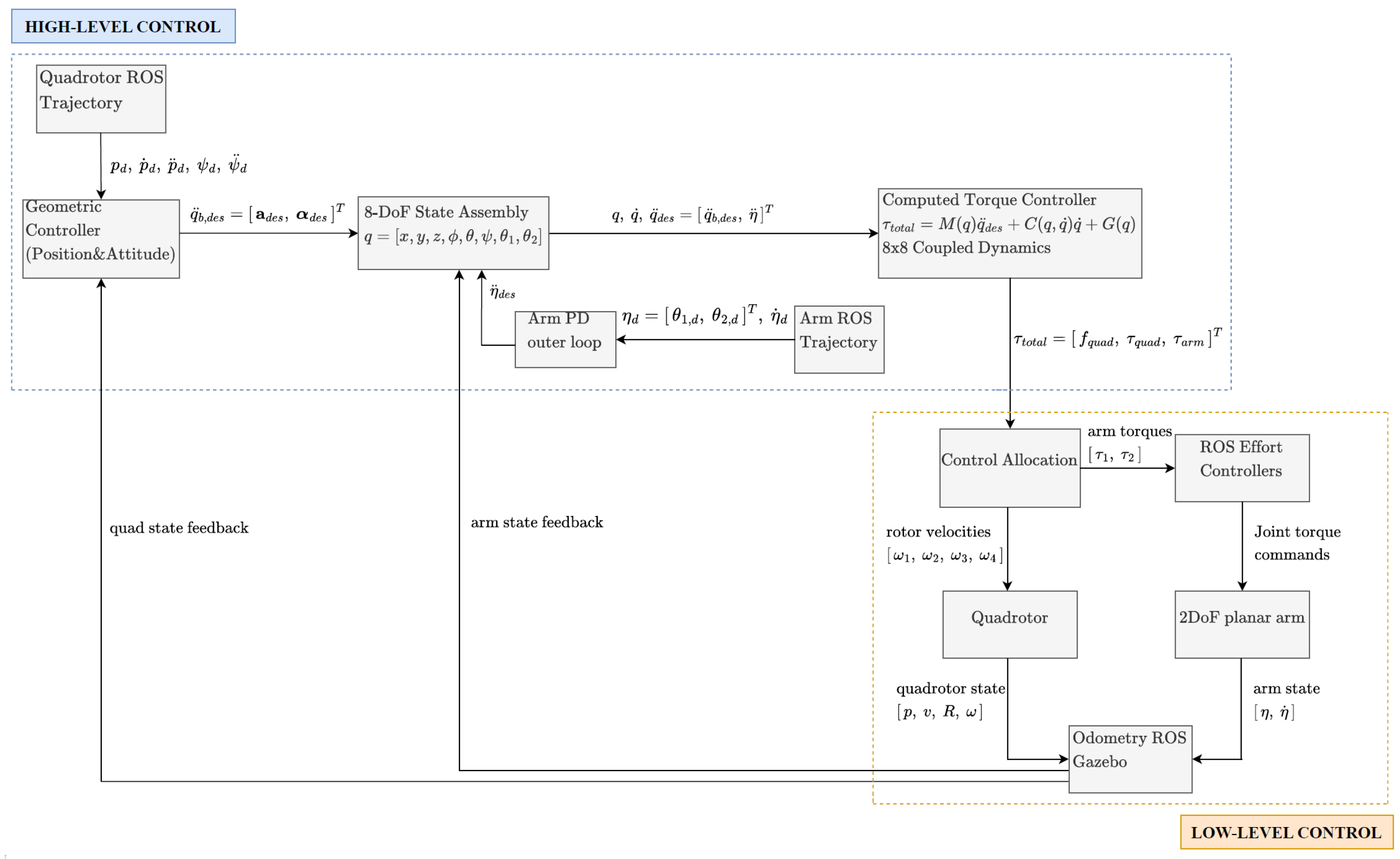
The aerial manipulation system employs a hybrid control strategy that combines the stability of geometric control [14,19] with the fully coupled computed torque control method. The architecture is designed to leverage geometric control error calculation, while computed torque control captures the complete 8-DOF E-L dynamics model between the quadrotor and the planar 2-DOF robotic arm. The geometric controller receives position and attitude references from the trajectory planner and computes desired accelerations ${\ddot{\mathbf{x}}}_{\mathrm{des}}$ and desired angular accelerations ω_acc,des using position errors e_p = x − x_d, velocity errors ${\mathbf{e}}_v=\dot{\mathbf{x}}-{\dot{\mathbf{x}}}_d$, and attitude errors derived from the SE(3) manifold. Additionally, a separate PD control law generates desired joint accelerations for the manipulator using joint position errors e_θ = θ_d − θ and joint velocity errors ${\mathbf{e}}_{\dot{\theta }}={\dot{\mathbf{\theta }}}_d-\dot{\mathbf{\theta }}$, computed as ${\ddot{\theta }}_{i,\mathrm{des}}=k_{p,i}{e}_{\theta ,i}+k_{d,i}{e}_{\dot{\theta },i}$ for each joint. The computed torque method then utilizes these combined outputs—geometric accelerations for the quadrotor and PD accelerations for the manipulator—as desired acceleration inputs ${\ddot{\mathbf{q}}}_{\mathrm{des}}$ for the full 8-DOF system, computing the required generalized forces through (49). This creates a hierarchical structure where geometric control provides reference trajectory tracking through error formulations, while the computed torque ensures proper handling of the system’s coupled dynamics through complete mass matrix, Coriolis, and gravity compensation.

In addition, a challenge encountered in pure computed torque implementations, as demonstrated in [13], is the requirement for desired roll and pitch angles in the quadrotor translational control law in the mass matrix computation, leading to approximations that compromise the unified dynamics model. The hybrid approach resolves this limitation by leveraging the geometric controller’s generation of desired attitude commands; the controller computes the required roll and pitch angles to achieve desired translational motion through thrust vectoring, eliminating the need for mass matrix approximations. The overall control architecture of the system is shown in Figure 2.

4.2. Geometric Controller

The geometric controller in RotorS [14] follows the approach of [19] for quadrotor control on SE(3), which provides singularity-free attitude representation and almost global stability guarantees. The term almost global refers to the fact that asymptotic stability holds for all initial attitude errors less than 180° [19].

Position Control: Translational dynamics control is based on position and velocity tracking errors defined in the world frame. The position error is computed as

$${\mathbf{e}}_p=\mathbf{p}-{\mathbf{p}}_d$$

(80)

where $\mathbf{p}\in {\mathbb{R}}^3$ represents the current quadrotor position and ${\mathbf{p}}_d\in {\mathbb{R}}^3$ is the desired position trajectory.

The velocity error requires transformation from the body-fixed frame to the world frame:

$${\mathbf{e}}_v=\mathbf{R}\mathbf{v}-{\mathbf{v}}_d$$

(81)

where R ∈ SO(3) is the rotation matrix from the body-fixed frame to the world frame, $\mathbf{v}\in {\mathbb{R}}^3$ is the body-fixed frame velocity, and ${\mathbf{v}}_d\in {\mathbb{R}}^3$ is the desired world frame velocity.

The desired acceleration is computed through a PD control law with gravity compensation as follows [14]:

$${\mathbf{a}}_d={\displaystyle \frac{1}{m}}({\mathbf{K}}_p{\mathbf{e}}_p+{\mathbf{K}}_v{\mathbf{e}}_v)-g{\mathbf{e}}_3-{\ddot{\mathbf{p}}}_d$$

(82)

where ${\mathbf{K}}_p,{\mathbf{K}}_v\in {\mathbb{R}}^{3\times 3}$ are positive definite gain matrices, g is gravitational acceleration, e₃ = [0, 0, 1]^T is the unit vector in the z-direction, and ${\ddot{\mathbf{p}}}_d$ is the desired acceleration feedforward term.

Attitude Control: The attitude control follows a geometric approach on SO(3), avoiding singularities inherent in Euler angle representations. The desired rotation matrix R_d ∈ SO(3) is constructed from the desired thrust direction and heading. A detailed derivation of the complete desired rotation matrix R_d can be found in [19].

The attitude error is computed using the following matrix-based error function that ensures almost global convergence:

$${\mathbf{E}}_R={\displaystyle \frac{1}{2}}({\mathbf{R}}_d^T\mathbf{R}-{\mathbf{R}}^T{\mathbf{R}}_d)$$

(83)

The attitude error vector ${\mathbf{e}}_R\in {\mathbb{R}}^3$ is extracted from the skew-symmetric matrix E_R using the vee operator.

The angular velocity error accounts for the desired angular velocity in the body-fixed frame, as follows:

$${\mathbf{e}}_{\omega }=\mathit{\omega }-{\mathbf{R}}^T{\mathbf{R}}_d{\mathit{\omega }}_d$$

(84)

where ${\mathit{\omega }}_d\in {\mathbb{R}}^3$ represents the desired angular velocity, containing the desired yaw rate.

The angular acceleration command is computed using proportional derivative control with an additional nonlinear term, as follows:

$${\mathbf{\alpha }}_d=-{\mathbf{K}}_R^{\mathrm{norm}}{\mathbf{e}}_R-{\mathbf{K}}_{\omega }^{\mathrm{norm}}{\mathbf{e}}_{\omega }$$

(85)

where ${\mathbf{K}}_R^{\mathrm{norm}}={\mathbf{K}}_R^T{\mathbf{I}}_b^{-1}$ and ${\mathbf{K}}_{\omega }^{\mathrm{norm}}={\mathbf{K}}_{\omega }^T{\mathbf{I}}_b^{-1}$ are normalized gains that make the tuning independent of the inertia matrix, and ${\mathbf{I}}_b\in {\mathbb{R}}^{3\times 3}$ is the quadrotor inertia matrix.

The RotorS implementation includes an additional term of the form ω × ω in the angular-acceleration command. Since ω × ω ≡ 0, this term does not affect the command and is omitted in (85) for clarity.

The geometric controller outputs a_d and α_d serve as the reference accelerations for the computed torque controller.

4.3. Computed Torque Controller

The computed torque controller implements the unified 8-DOF E-L dynamics of the coupled quadrotor–manipulator system to generate model-consistent control inputs for trajectory tracking. While the control allocation follows the RotorS framework, the generalized forces supplied to the allocator are computed from the full coupled dynamics model derived in Section 3.

Control Law Formulation: For the unified system dynamics expressed in Equation (49) and no external disturbances, the general computed torque control law is [13]

$$\mathit{\tau }=\mathbf{M}(\mathbf{q})\mathbf{v}+\mathbf{C}(\mathbf{q},\dot{\mathbf{q}})\dot{\mathbf{q}}+\mathbf{G}(\mathbf{q})$$

(86)

where v is the auxiliary control input defined as

$$\mathbf{v}={\ddot{\mathbf{q}}}_d+{\mathbf{K}}_d\dot{\mathbf{e}}+{\mathbf{K}}_p\mathbf{e}$$

(87)

In this equation, e = q_d − q is the tracking error, and K_p, K_d are positive definite gain matrices.

Hybrid Control Strategy: In the proposed hybrid architecture, the auxiliary control input v is not constructed explicitly using joint-space error feedback. Instead, the desired acceleration vector ${\ddot{\mathbf{q}}}_{\mathrm{des}}$ is generated externally by combining the geometric controller for the quadrotor and PD control laws for the manipulator joints. These accelerations are then injected directly into the inverse dynamics model. This approach preserves the model-based feedforward compensation properties of computed torque control while allowing the use of well-established geometric error formulations for quadrotor motion. This substitution yields the following proposed control law:

$${\mathit{\tau }}_{\mathrm{total}}=\mathbf{M}(\mathbf{q}){\ddot{\mathbf{q}}}_{\mathrm{des}}+\mathbf{C}(\mathbf{q},\dot{\mathbf{q}})\dot{\mathbf{q}}+\mathbf{G}(\mathbf{q})$$

(88)

where ${\ddot{\mathbf{q}}}_{\mathrm{des}}\in {\mathbb{R}}^8$ is the desired acceleration vector for the coupled system.

The generalized coordinate vector is partitioned as

$$\mathbf{q}=\left[\begin{array}{c}{\mathbf{q}}_b\\ \mathit{\eta }\end{array}\right],{\mathbf{q}}_b=\left[\begin{array}{c}\mathbf{p}\\ \mathbf{\Phi }\end{array}\right]$$

(89)

where p = [x, y, z]^T is the quadrotor position expressed in the inertial frame, Φ = [ϕ, θ, ψ]^T are the quadrotor Euler angles, and η = [θ₁, θ₂]^T are the manipulator joint angles.

The desired acceleration vector ${\ddot{\mathbf{q}}}_{\mathrm{des}}$ is constructed by combining quadrotor and manipulator reference accelerations, as follows:

$${\ddot{\mathbf{q}}}_{\mathrm{des}}=\left[\begin{array}{c}{\ddot{\mathbf{q}}}_{b,\mathrm{des}}\\ {\ddot{\mathit{\eta }}}_{\mathrm{des}}\end{array}\right]$$

(90)

The quadrotor desired accelerations are generated by the geometric controller as

$${\ddot{\mathbf{q}}}_{b,\mathrm{des}}=\left[\begin{array}{c}{\mathbf{a}}_{d,\mathrm{geo}}\\ {\mathit{\alpha }}_{d,\mathrm{geo}}\end{array}\right]$$

(91)

where a_d,geo and α_d,geo are computed using Equations (82) and (85), respectively. These accelerations encode position, velocity, and attitude tracking errors expressed directly on the SE(3) manifold.

Desired joint accelerations for the planar 2-DoF manipulator are generated using independent PD control laws, as follows:

$${\ddot{\mathit{\eta }}}_{\mathrm{des}}=\left[\begin{array}{c}{k}_{p,1}({\theta }_{1,d}-{\theta }_1)+k_{d,1}({\dot{\theta }}_{1,d}-{\dot{\theta }}_1)\\ k_{p,2}({\theta }_{2,d}-{\theta }_2)+k_{d,2}({\dot{\theta }}_{2,d}-{\dot{\theta }}_2)\end{array}\right]$$

(92)

The generalized control input computed from the inverse dynamics, ${\mathit{\tau }}_{\mathrm{total}}\in {\mathbb{R}}^8$, is partitioned according to the base and arm coordinates $\mathbf{q}={[{\mathbf{q}}_b^T,{\mathit{\eta }}^T]}^T$, where ${\mathbf{q}}_b\in {\mathbb{R}}^6$ and $\mathit{\eta }\in {\mathbb{R}}^2$, as follows:

$${\mathit{\tau }}_{\mathrm{total}}=\left[\begin{array}{c}{\mathbf{u}}_b\\ {\mathit{\tau }}_{\mathrm{arm}}\end{array}\right],{\mathbf{u}}_b=\left[\begin{array}{c}{\mathbf{f}}_{\mathrm{W}}\\ {\mathit{\tau }}_{\mathrm{\Phi }}\end{array}\right]$$

(93)

Here, ${\mathbf{f}}_{\mathrm{W}}\in {\mathbb{R}}^3$ is a virtual inertial-frame force and ${\mathit{\tau }}_{\mathrm{\Phi }}\in {\mathbb{R}}^3$ is the generalized rotational force to the Euler-rate vector $\dot{\mathbf{\Phi }}$. Since the quadrotor is underactuated, only the thrust component along the body-fixed z-axis is realizable; therefore, the commanded thrust is obtained by projecting f_b onto the body-fixed z-axis, while the corresponding body-frame torque τ_quad = Q^−Tτ_Φ is allocated to the rotors. The arm torque command is ${\mathit{\tau }}_{\mathrm{arm}}={[{\tau }_{{\theta }_1},{\tau }_{{\theta }_2}]}^T$.

The unified E-L model is written in generalized coordinates as $\mathbf{q}={[{\mathbf{p}}^T,{\mathbf{\Phi }}^T,{\mathit{\eta }}^T]}^T$; hence, the rotational generalized forces ${\mathit{\tau }}_{\mathrm{\Phi }}\in {\mathbb{R}}^3$ are connected to the Euler-rate vector $\dot{\mathbf{\Phi }}$. However, the multirotor rotational dynamics and control allocation are naturally expressed in the body-fixed frame in terms of the body torque τ_quad and body angular acceleration ${\dot{\mathit{\omega }}}_b$. Using (3), the virtual moment yields:

$${\mathit{\tau }}_{\mathrm{\Phi }}=\mathbf{Q}{(\varphi ,\theta )}^T{\mathit{\tau }}_{\mathrm{quad}},{\mathit{\tau }}_{\mathrm{quad}}=\mathbf{Q}{(\varphi ,\theta )}^{-T}{\mathit{\tau }}_{\mathrm{\Phi }}$$

(94)

Similarly, differentiating (3) gives the acceleration mapping

$$\begin{array}{cc}\hfill {\dot{\mathit{\omega }}}_b& =\mathbf{Q}(\varphi ,\theta )\ddot{\mathbf{\Phi }}+\dot{\mathbf{Q}}(\varphi ,\theta )\dot{\mathbf{\Phi }},\hfill \\ \hfill \ddot{\mathbf{\Phi }}& =\mathbf{Q}{(\varphi ,\theta )}^{-1}\left({\dot{\mathit{\omega }}}_b-\dot{\mathbf{Q}}(\varphi ,\theta )\dot{\mathbf{\Phi }}\right)\hfill \end{array}$$

(95)

Equations (94) and (95) are used to interface the Euler-angle inverse dynamics model with the RotorS allocation, which expects body moments.

Note that the RotorS mixer is parameterized by a matrix that maps the vector ${[{\mathit{\alpha }}_b^T,f_z]}^T$ to squared rotor speeds, where α_b is an inertia-normalized moment command (units of rad/s²). In our implementation, the inverse dynamics model yields the generalized Euler torque τ_Φ, which is converted to the body torque τ_quad = Q^−Tτ_Φ and then normalized as ${\mathit{\alpha }}_b={\mathbf{I}}_b^{-1}{\mathit{\tau }}_{\mathrm{quad}}$ before being passed to the mixer.

4.4. Control Allocation

The control allocation translates the computed generalized forces from the coupled dynamics equations into actuator commands for the 8-DOF system. This implementation takes the total system forces and torques computed by the computed torque controller and distributes them between the quadrotor rotors (four actuator outputs) and manipulator joints (two actuator outputs). This creates six independent control inputs for an 8-DOF system, resulting in an underactuated configuration where the quadrotor’s lateral forces f_x and f_y must be generated indirectly through attitude control rather than direct actuation.

Quadrotor Allocation: The quadrotor allocation follows the RotorS framework implementation [14], which builds upon Lee’s geometric control foundation [19]. The allocation matrix maps desired body torques and total thrust to individual rotor velocities through the following dynamically generated configuration matrix:

$$\left[\begin{array}{c}{\tau }_x\\ {\tau }_y\\ {\tau }_z\\ f_z\end{array}\right]={\mathbf{A}}_m\left[\begin{array}{c}{\omega }_1^2\\ {\omega }_2^2\\ {\omega }_3^2\\ {\omega }_4^2\end{array}\right]$$

(96)

where f_z represents the total thrust generated by the system, τ denotes the torques acting on the center of gravity, and ω_i are the individual rotor angular velocities. The allocation matrix ${\mathbf{A}}_m\in {\mathbb{R}}^{4\times 4}$ is constructed from the following quadrotor configuration:

$${\mathbf{A}}_m=\left[\begin{array}{cccc}{c}_T& c_T& c_T& c_T\\ 0& d{c}_T& 0& -d{c}_T\\ -d{c}_T& 0& d{c}_T& 0\\ -c_T{c}_M& c_T{c}_M& -c_T{c}_M& c_T{c}_M\end{array}\right]$$

(97)

where c_T is the rotor thrust coefficient, c_M is the rotor moment coefficient relating the thrust to drag moment, and d is the distance from the vehicle center of mass to each rotor.

The rotor velocities are computed using the Moore–Penrose pseudo-inverse

$$\left[\begin{array}{c}{\omega }_1^2\\ {\omega }_2^2\\ {\omega }_3^2\\ {\omega }_4^2\end{array}\right]={\mathbf{A}}_m^{†}\left[\begin{array}{c}{\tau }_x\\ {\tau }_y\\ {\tau }_z\\ f_z\end{array}\right]$$

(98)

The rotor speed mapping in RotorS is implemented at the acceleration level as

$$\left[\begin{array}{c}\mathit{\tau }\\ f_z\end{array}\right]=\left({\mathbf{A}}_m^{†}\mathrm{diag}(\mathbb{I},1)\right)\left[\begin{array}{c}\mathbf{\alpha }\\ f_z\end{array}\right]$$

(99)

Thus, the RotorS allocator expects commanded angular acceleration and thrust, while the inverse dynamics model outputs generalized base wrench components (f_W, τ_quad). Therefore, the computed base wrench is converted into

$$\begin{array}{cc}\hfill {\mathit{\omega }}_{\mathrm{acc}}& ={\mathbf{I}}_b^{-1}{\mathit{\tau }}_{\mathrm{quad}}\hfill \end{array}$$

(100)

$$\begin{array}{cc}\hfill f_z& =-{\mathbf{f}}_{\mathrm{W}}·{\widehat{\mathbf{z}}}_{\mathrm{body}}\hfill \end{array}$$

(101)

where I_b is the quadrotor inertia matrix, τ_quad are the quadrotor torques from the computed torque, and f_W are the quadrotor forces projected onto the body-fixed z-axis to obtain thrust.

Manipulator Allocation: The computed joint torques from the unified dynamics are directly commanded to the joint motors (i.e., direct torque control) using ROS effort controllers. The manipulator joint torques are extracted from the total control vector from Equation (93).

The extracted torques are directly commanded to the joint motors with the following safety limits:

$${\tau }_{1,cmd}={\tau }_{{\theta }_1}$$

(102)

$${\tau }_{2,cmd}={\tau }_{{\theta }_2}$$

(103)

with actuator saturation applied to ensure $|{\tau }_{i,cmd}| \le 0.5$ Nm for safety. This limit is physically justified by the system parameters; given the link masses m₁ = m₂ = 0.04 kg, link lengths L₁ = L₂ = 0.15 m, and end-effector mass m_ee = 0.01 kg, the maximum static gravity torque at Joint 1 with both links fully extended horizontally is approximately τ_max ≈ (m₁L₁/2 + m₂L₁ + m_eeL₁)g ≈ 0.11 Nm, giving a safety margin of 4.5× over the maximum expected static load, consistent with lightweight servo actuator specifications for manipulators of this scale. When saturation becomes active in more aggressive trajectory scenarios, standard anti-windup strategies such as command scaling and torque prioritization would be required to prevent integrator windup and maintain stability.

It is worth noting that torque-level joint control, as implemented here via ROS effort controllers, is practically realizable using modern servo actuators such as the Dynamixel series operating in the current control mode.

5. Simulated Experiments

This section evaluates the influence of dynamic coupling between a quadrotor and a 2-DoF planar manipulator on tracking performance. The aerial manipulation platform consists of a Hummingbird quadrotor rigidly attached to a two-link planar arm (rod geometry), as illustrated in Figure 1. All simulated experiments are conducted in the RotorS simulator [14] using the Gazebo physics engine.

Table 1. System parameters.

Parameter	Symbol	Value
Quadrotor
Quadrotor mass	mb	0.716 kg
Quadrotor inertia (x, y)	Ixx, Iyy	7.0 × 10−3 kg·m2
Quadrotor inertia (z)	Izz	1.2 × 10−2 kg·m2
Rotor thrust coefficient	cT	8.549 × 10−6 N·s2/rad2
Rotor moment coefficient	cM	1.6 × 10−2 m
Rotor-to-CoM distance	d	0.17 m
Rotor drag coefficient	cD	8.064 × 10−5
Manipulator
Link 1 mass	m1	0.04 kg
Link 2 mass	m2	0.04 kg
End-effector mass	mee	0.01 kg
Link 1 length	L1	0.15 m
Link 2 length	L2	0.15 m
Link 1 CoM distance	lc1	0.075 m
Link 2 CoM distance	lc2	0.075 m
Link 1 moment of inertia	I1,yy	7.5 × 10−5 kg·m2
Link 2 moment of inertia	I2,yy	7.5 × 10−5 kg·m2

presents the system parameters used in all simulated experiments. It should be noted that the results presented in this work are specific to the 2-DOF planar manipulator configuration with the parameters given in Table 1.

To evaluate the effectiveness of the proposed control strategy, three simulation test cases of increasing complexity are conducted. The objective is to assess the impact of dynamic coupling between the quadrotor and the manipulator by comparing the fully coupled E-L model with the hybrid controller to the geometric controller with a decoupled PD controller with gravity compensation for the arm. Both platforms share identical physical parameters. The quadrotor geometric controller gains (K_p, K_v, K_R, K_ω) are the default pre-tuned gains provided by the RotorS simulator for the Hummingbird platform [14], kept identical for both controllers to ensure a fair comparison. The manipulator joint gains k_p,i and k_d,i were tuned independently for each controller following Appendix A. Both controllers run at 200 Hz; reference commands are published at 50 Hz.

Table 2. Expanded metric comparison between all test cases. Steady-state metrics computed over t ∈ [10, 20] s; transient metrics computed over t ∈ [0, 8] s; IAE computed over full run. Bold indicates better-performing controller.

	Case 1: Ramp		Case 2: Trajectory		Case 3: Aerial
Metric	CT	PD	CT	PD	CT	PD
Steady-state metrics
Joint error mean [rad]	0.019	0.057	0.036	0.049	0.012	0.031
Joint error max [rad]	0.265	0.300	0.105	0.073	0.025	0.039
Drone pos mean [m]	0.040	0.083	0.031	0.065	0.035	0.053
Drone pos max [m]	0.076	0.140	0.034	0.089	0.038	0.083
EE error mean [m]	–	–	–	–	0.036	0.066
EE error max [m]	–	–	–	–	0.041	0.113
Pitch RMS [rad]	0.026	0.012	0.010	0.056	0.010	0.039
Roll RMS [rad]	0.0002	0.0001	0.0001	0.0007	0.006	0.007
τ1 RMS [Nm]	0.036	0.041	0.045	0.056	0.030	0.033
τ2 RMS [Nm]	0.012	0.010	0.010	0.009	0.006	0.006
Transient and integrated metrics
Peak pitch trans. [rad]	0.130	0.012	0.227	0.003	0.245	0.012
Peak pos trans. [m]	0.088	0.035	0.099	0.037	0.302	0.303
Settling time [s]	<10	<10	10	23.5	10	24.5
IAE pos [m·s]	1.17	2.33	0.94	1.47	2.94	3.89
IAE joint [rad·s]	2.17	3.68	2.42	2.62	1.26	1.99

presents the quantitative results. Bold values indicate the better-performing controller for each metric. Metrics are computed over the steady-state interval (t ∈ [10, 20] s), excluding the initial transients. Throughout this section and in all figures and tables, CT refers to the proposed hybrid geometric computed torque controller derived in Section 4, and PD refers to the baseline decoupled controller consisting of the standard RotorS geometric controller for the quadrotor base and independent PD control with gravity compensation for the manipulator joints. The CT controller receives position, velocity, and acceleration feedforward references for both the quadrotor and manipulator joints, while the PD controller receives only position and velocity references, as acceleration feedforward cannot be meaningfully utilized within a decoupled direct-torque architecture.

Both controllers receive identical trajectory commands at t = 0.01 s from identical initial conditions (θ₁ = θ₂ = 0 rad), verified from the recorded bag files. The delay observed in the PD controller response across all cases reflects the decoupled architecture’s limitation. When arm motion begins, inertial coupling forces a disturbance in the quadrotor attitude, and since the PD controller has no knowledge of this coupling, the quadrotor attitude loop must reactively settle before accurate joint tracking is possible. The CT controller avoids this by generating anticipatory attitude adjustments through M_qη, pre-compensating the coupling forces.

All three case studies are conducted under nominal conditions with no external disturbances, consistent with the assumptions under which the CT controller is derived (Section 4.3). To assess the effect of disturbances on both controllers, two additional wind robustness experiments are conducted at the end of Case 2 and Case 3, in which a lateral wind gust is applied during the arm trajectory execution and a constant wind is applied during the aerial manipulation case. These experiments are not intended to demonstrate robustness of the CT controller but to characterize the comparative performance degradation of the coupled versus decoupled architectures when the no-disturbance assumption is violated.

5.1. Case 1: Hovering Quadrotor with Arm Ramp Response

As an initial validation experiment, a joint-space ramp trajectory is applied to the first arm joint while the second joint is held fixed at zero. This experiment is designed to evaluate joint-level tracking performance and showcase coupling effects between the manipulator and the quadrotor base under static flight conditions.

Joint1 is commanded to move between symmetric angular limits using smooth ramp transitions, while Joint2 remains fixed throughout the experiment. The quadrotor hovers at a fixed position p_d = (0, 0, 1), while the arm executes a sequence of ramp commands in θ₁. Starting from the equilibrium configuration (θ₁, θ₂) = (0, 0), Joint1 is ramped (over 1 s) to its positive limit θ₁ = +0.3 rad and held for 5 s, returned to center, then ramped to θ₁ = −0.3 rad and held for 5 s before returning to center. Joint2 remains at θ₂ = 0 throughout. This sequence is executed once.

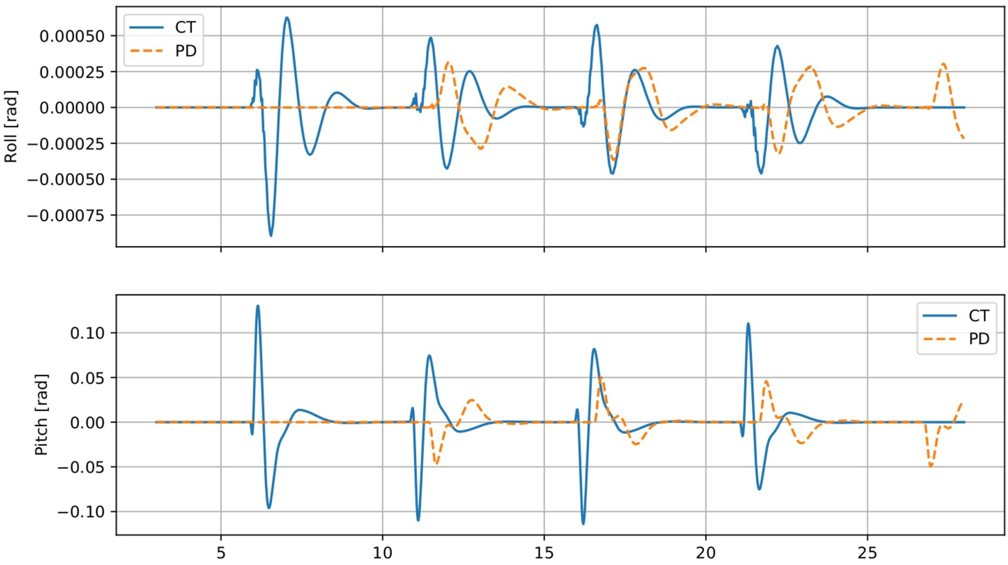
Figure 3 shows the quadrotor orientation during Case 1. The CT controller exhibits larger transient pitch excursions (±0.13 rad) during the ramp transitions, compared to ±0.03 rad for the PD controller. This behavior arises from the coupled system dynamics; the CT controller generates anticipatory attitude adjustments through the off-diagonal terms of the mass matrix to accelerate the arm joint toward the commanded set point, resulting in a 66% reduction in the mean joint tracking error (Table 2). Between transitions, the CT controller returns to near-zero pitch more rapidly than the PD controller. This trade-off between transient attitude deviations and improved joint tracking accuracy is inherent to the coupled control strategy.

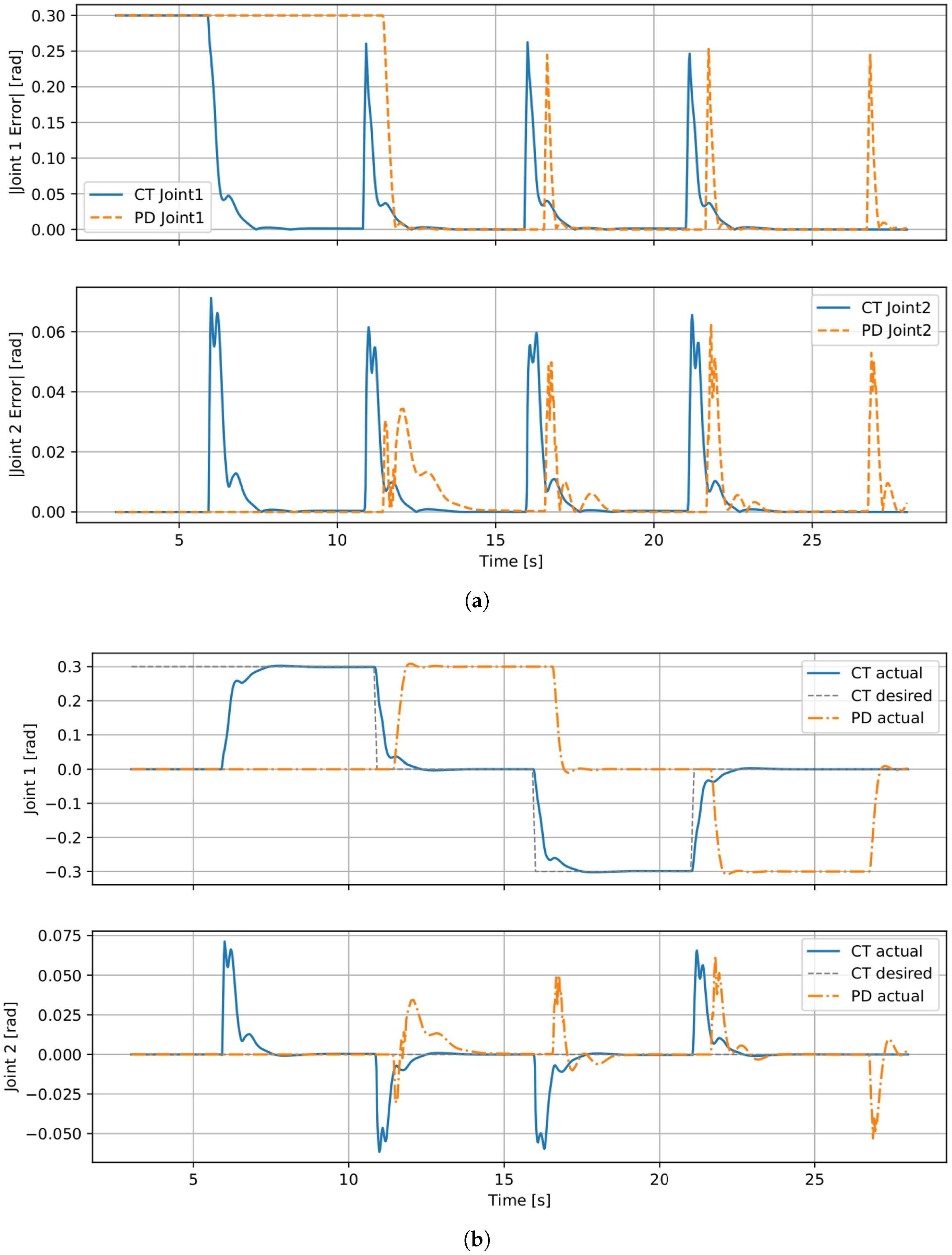
Figure 4b shows the joint angle response during Case 1. The CT controller tracks the ramp reference with minimal delay, reaching the commanded ±0.3 rad within approximately 2 s of ramp completion, whereas the PD controller requires approximately 5 s to converge to each set point. Joint2, which is commanded to remain at zero, exhibits transient coupling disturbances during each Joint1 transition for both controllers. However, the CT controller recovers more rapidly due to the cross-coupling compensation incorporated in the mass matrix. Figure 4a confirms these observations, demonstrating that the CT controller achieves near-zero steady-state error between transitions, while the PD controller exhibits prolonged settling.

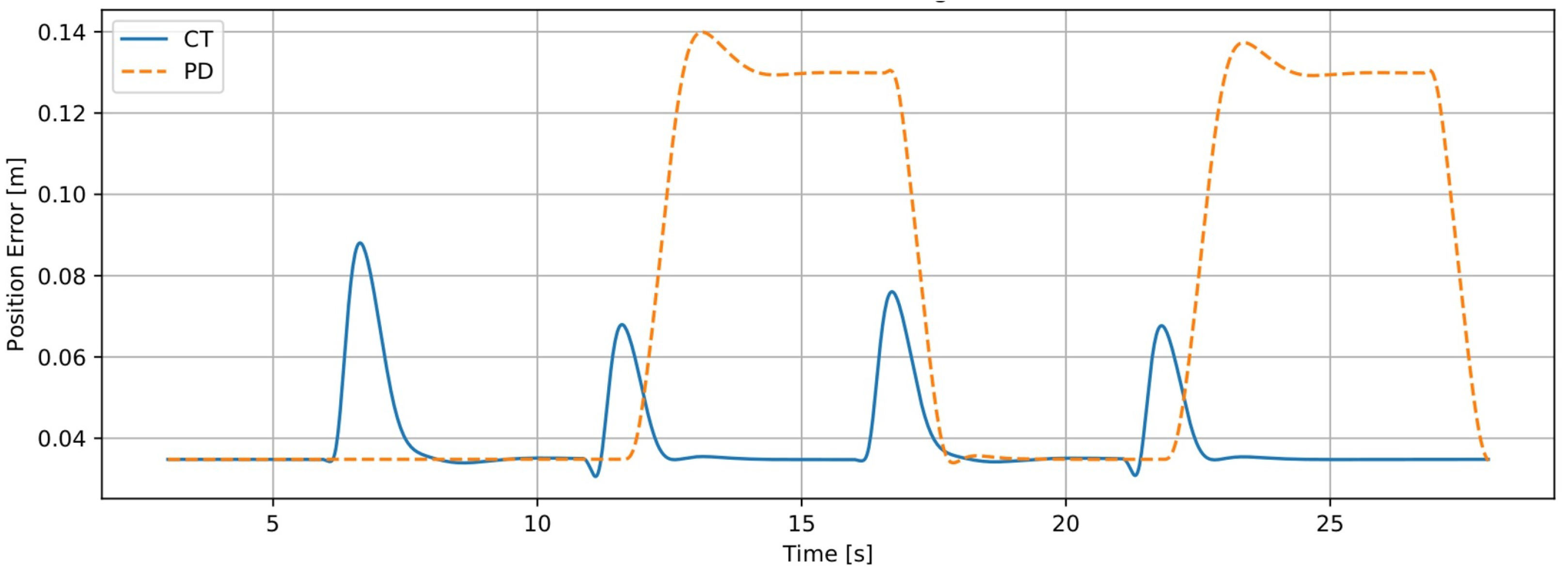
Figure 5 shows the quadrotor position tracking error during Case 1. The CT controller exhibits brief transient peaks in the range of 0.07–0.09 m during the ramp transitions, returning to the baseline hovering error of approximately 0.035 m within 2 s. In contrast, the PD controller accumulates a sustained position error of 0.13–0.14 m while the arm is held at ±0.3 rad. This error arises from the shifted center of mass, which the decoupled position controller cannot compensate.

5.2. Case 2: Hovering Quadrotor with Arm Trajectory Tracking

In the second experiment, the quadrotor again hovers at p_d = (0, 0, 1) m while both arm joints simultaneously track the smooth sinusoidal references

$$\begin{array}{cc}\hfill {\theta }_{1,d}(t)& =0.3sin(2\pi ·0.5t),\hfill \end{array}$$

(104)

$$\begin{array}{cc}\hfill {\theta }_{2,d}(t)& =0.2sin(2\pi ·0.5t+\frac{\pi }{2}),\hfill \end{array}$$

(105)

with velocity and acceleration feedforward supplied to the CT controller. The PD method receives only the position and velocity references. The trajectory lasts 15 s, after which both joints return to zero. This scenario excites the full Coriolis and centrifugal coupling between the arm’s degrees of freedom and the quadrotor attitude at a frequency (0.5 Hz). The phase offset between the two joints ensures that the combined center-of-mass motion is not purely planar, stressing the cross-coupling compensation.

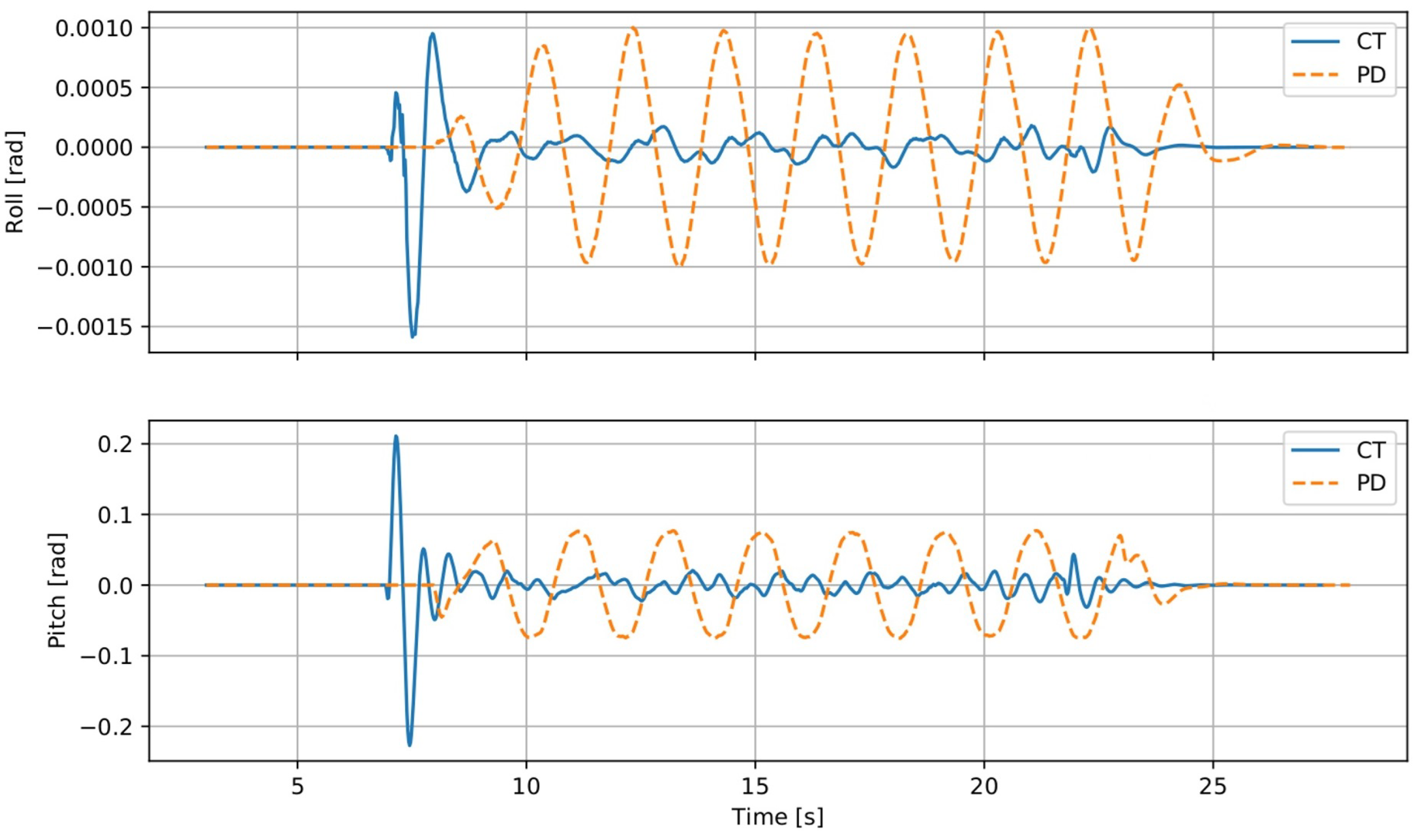
Figure 6 shows the quadrotor orientation. The pitch axis, which is directly coupled to the arm motion through the planar kinematic chain, exhibits the most significant difference between the two controllers. During steady-state tracking (t ∈ [10, 25] s), the CT controller maintains pitch oscillations below 0.02 rad, whereas the PD controller exhibits sustained oscillations of approximately ±0.07 rad at the arm trajectory frequency. Roll disturbances remain negligible for both controllers (on the order of 10⁻³ rad), consistent with the planar geometry of the manipulator.

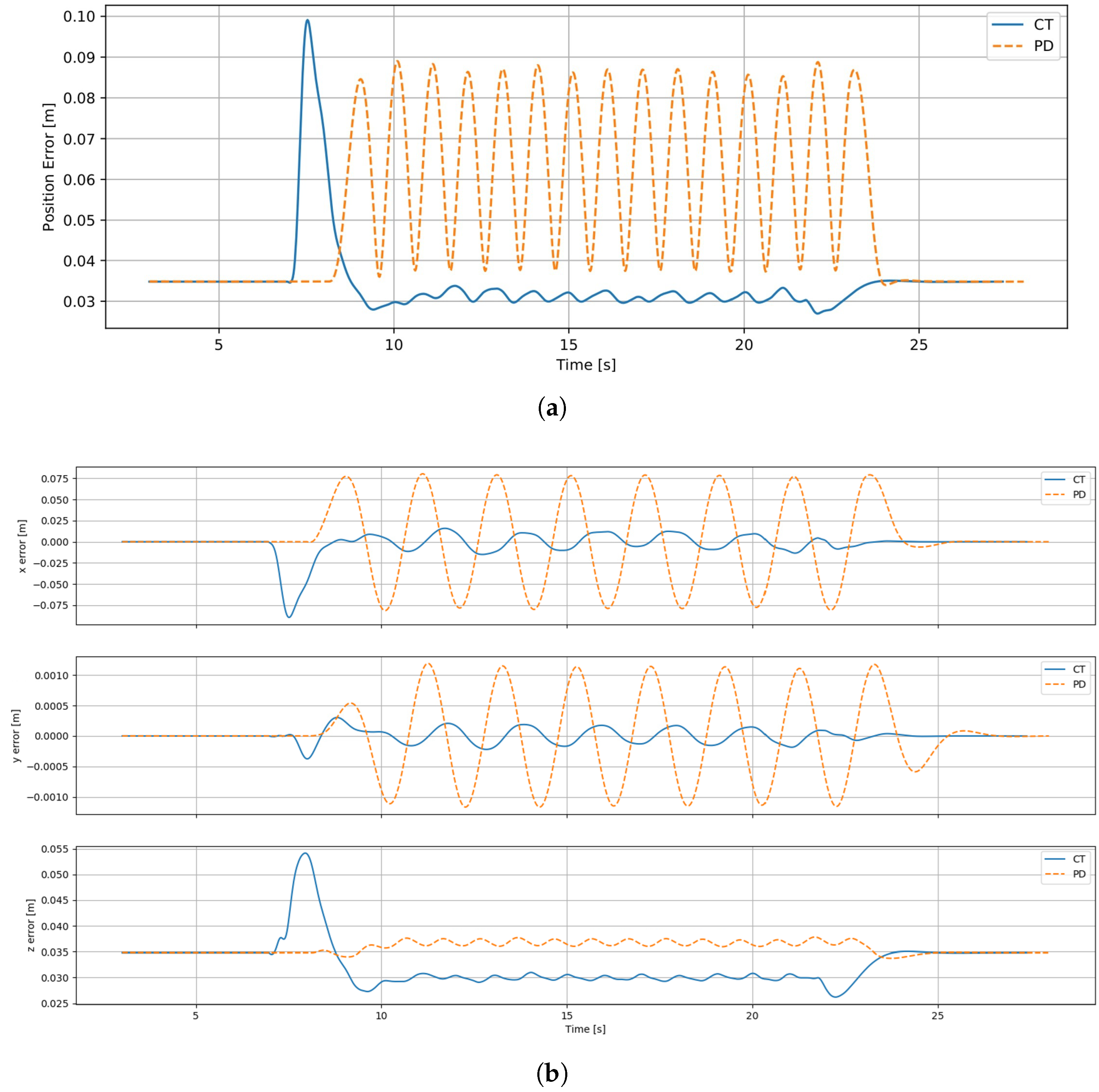
Figure 7a shows the quadrotor position tracking error norm and Figure 7b shows the quadrotor position tracking error per axis (x, y, z) with CT and PD overlaid during Case 2. Prior to the arm trajectory (t < 6 s), both controllers maintain comparable hovering accuracy of approximately 0.035 m, attributable to a steady-state altitude offset induced by the additional manipulator weight. Once the arm motion begins, the PD controller exhibits oscillations in the range of 0.04–0.09 m at the arm trajectory frequency (0.5 Hz) mostly along the x-axis, consistent with the pitch coupling induced by the planar arm motion: the uncompensated arm swing produces periodic pitch disturbances that drive translational drift in x. The CT controller maintains near-zero x and y errors during the steady state, while the z-axis offset remains comparable between both controllers.

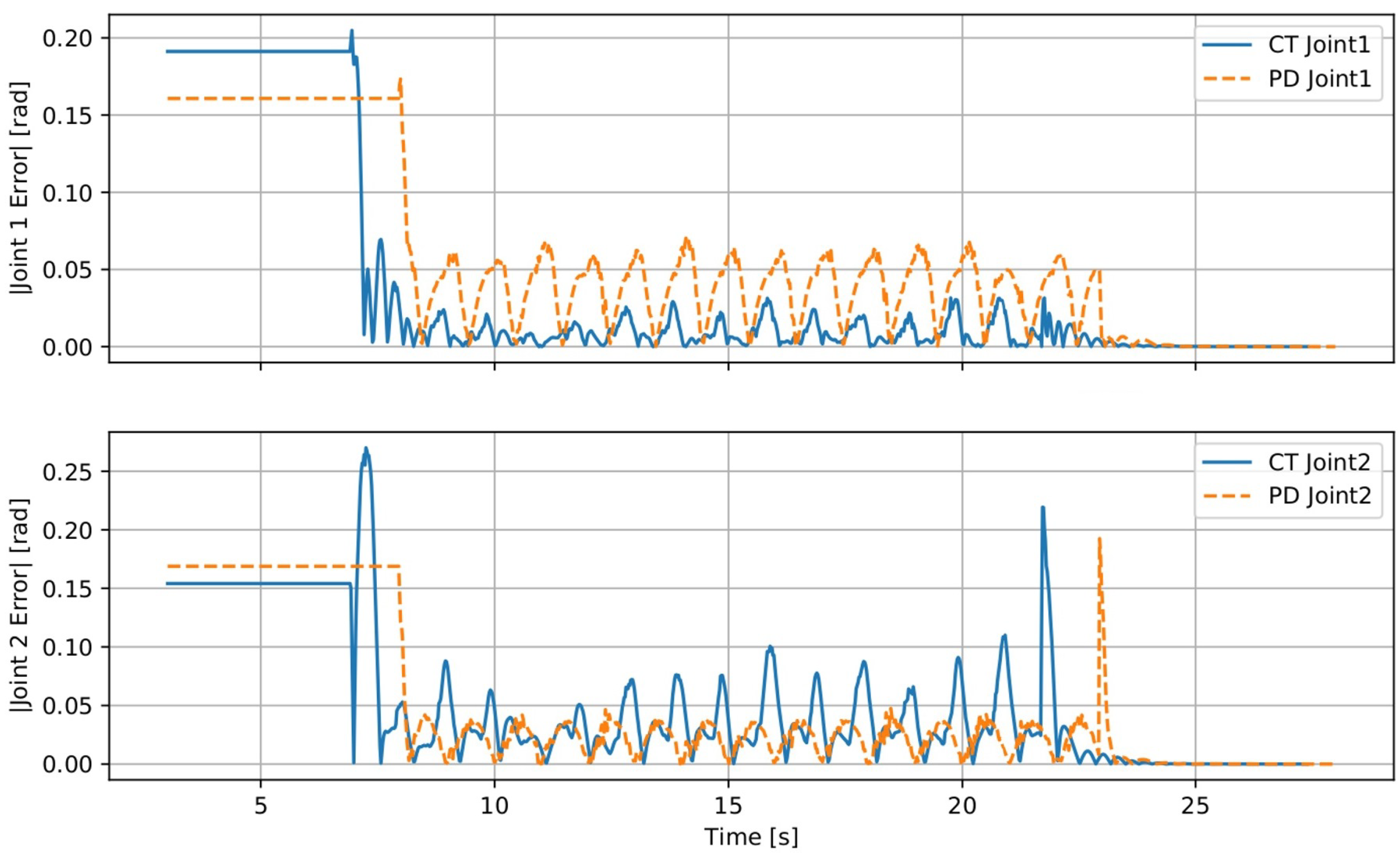
Figure 8 shows the joint tracking errors during Case 2. Joint1 exhibits a noticeable difference between the two controllers, with the CT controller maintaining errors below 0.02 rad, whereas the PD controller displays persistent oscillations within the range of 0.04–0.06 rad. Case 2 employs larger arm trajectory amplitudes (0.3 rad and 0.2 rad) compared to Case 3 (0.2 rad and 0.15 rad), resulting in higher peak joint velocities and, consequently, stronger Coriolis coupling forces. This increase in dynamic coupling accounts for the larger Joint2 tracking errors observed in this scenario. The 82% reduction in pitch RMS (Table 2) is directly attributable to the Coriolis coupling block C_qη, which captures the periodic disturbance torques induced by the 0.5 Hz sinusoidal arm trajectory and preemptively compensates them before they propagate to the quadrotor attitude loop. The PD controller, lacking this term, cannot anticipate these disturbances and exhibits sustained pitch oscillations at the arm trajectory frequency.

Robustness to Wind Disturbance

To assess robustness to external aerodynamic disturbances, the Case 2 scenario is repeated under a simulated lateral wind gust of 2 m/s applied along the world-frame x-axis for a duration of 3 s, injected at t = 7.5 s during the sinusoidal arm trajectory execution. The gust is generated using the RotorS Gazebo wind plugin applied to the quadrotor base link, with identical conditions for both controllers. No disturbance observer or wind feedforward term is present in either controller; the comparison therefore isolates the inherent disturbance rejection arising from the coupled versus decoupled dynamic compensation architectures. Both controllers experience performance degradation under the disturbance, as expected since the CT controller is derived under the assumption of no external disturbances (Section 4.3).

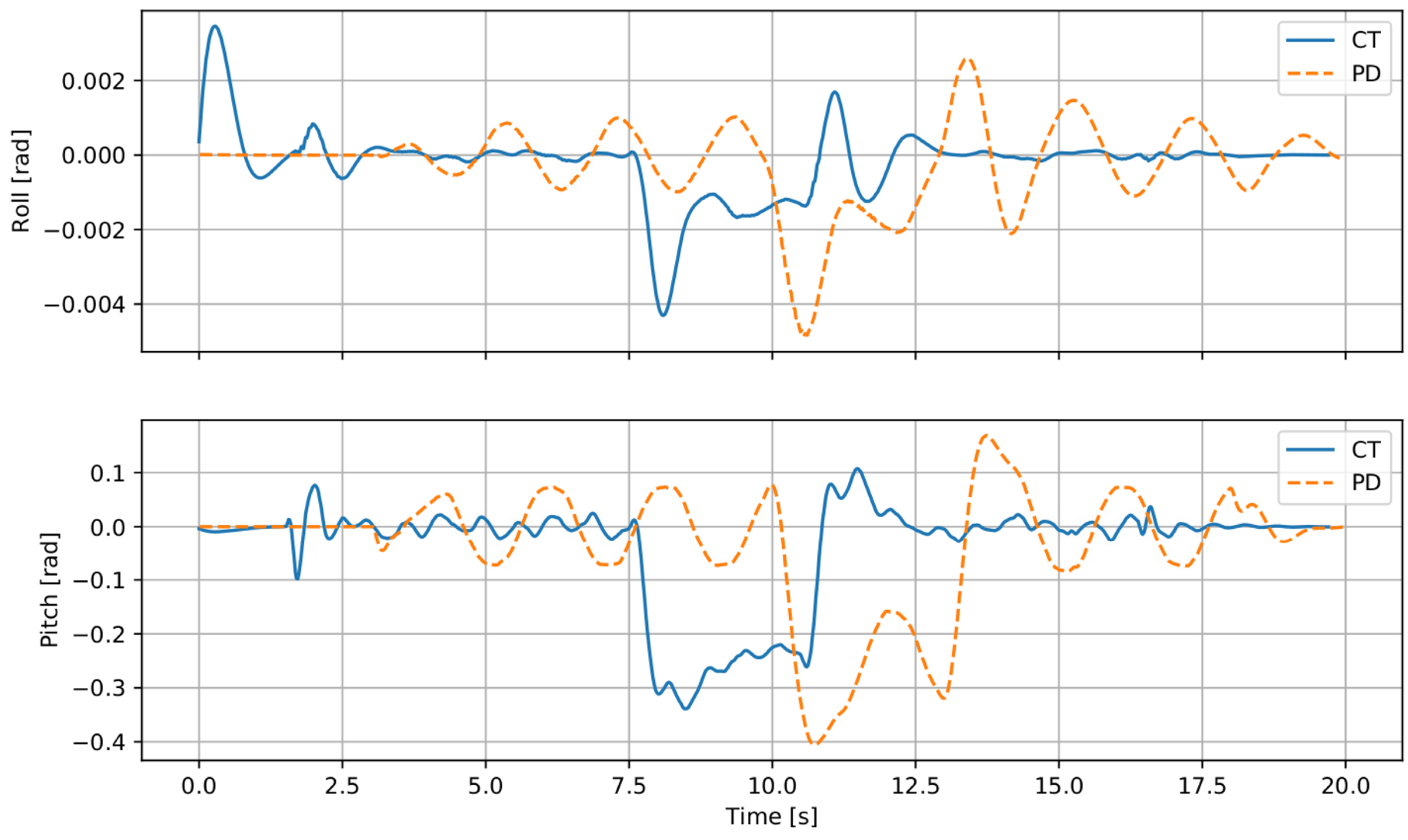
Figure 9 shows the quadrotor pitch during the wind experiment. At gust onset, the CT controller generates an immediate corrective pitch response through the coupled inverse dynamics, producing a transient peak of −0.32 rad that resolves within approximately 3 s of gust termination. The PD controller responds reactively through the geometric attitude loop alone, reaching a larger peak of −0.40 rad and sustaining oscillations for a further 5 s as the uncompensated arm coupling continuously re-excites the pitch channel at the arm trajectory frequency (0.5 Hz).

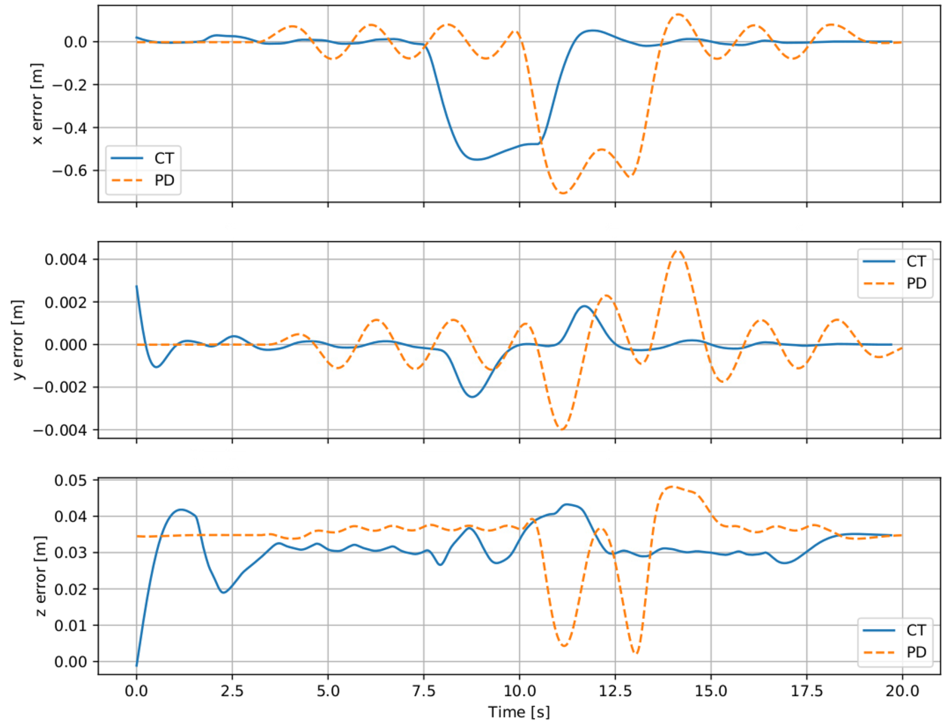
Figure 10 decomposes the position error by axis. CT reduces the peak x-axis error from 0.71 m (PD) to 0.55 m and achieves a 23% reduction in mean position error over the post-gust interval. The PD controller cannot suppress the x-axis oscillations because the uncompensated periodic arm swing continuously regenerates pitch coupling disturbances that drive x-axis drift—an interaction captured by C_qη in the CT formulation but absent from the decoupled PD architecture.

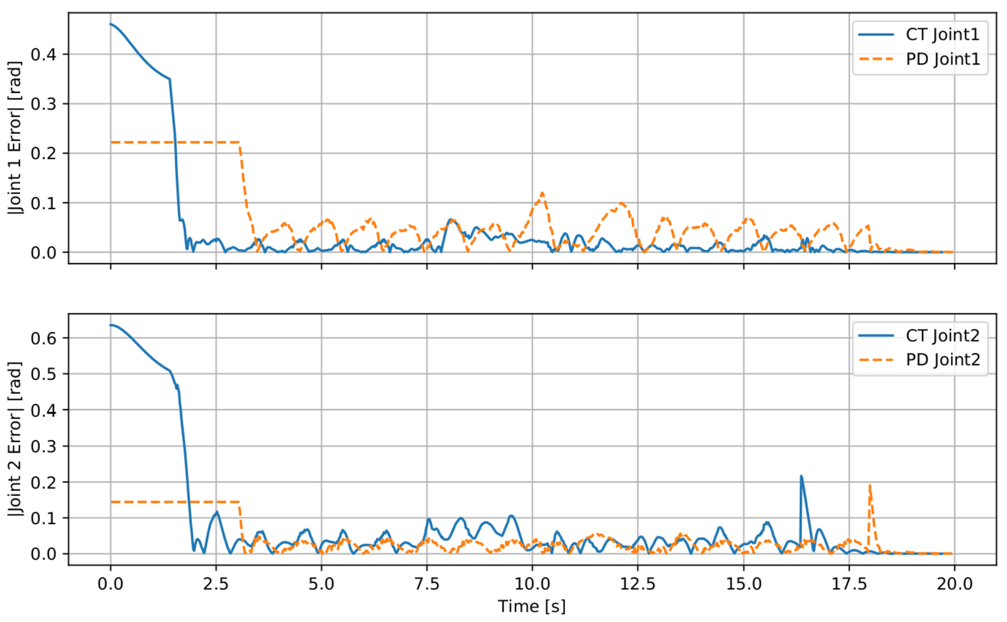
Figure 11 shows the joint tracking errors. Joint 1 under CT converges rapidly after the startup transient and remains near zero throughout the gust and recovery, while PD exhibits persistent oscillations driven by uncompensated coupling between arm motion and post-gust attitude transients. The CT startup transient on Joint 1 arises from the coupled inverse dynamics generating large initial torque commands as the full 8-DOF system accelerates from rest and is unrelated to the wind disturbance injected at t = 7.5 s. Joint 2 presents the inherent trade-off of the coupled architecture discussed in the caption; future work will address this through disturbance observer integration and selective joint decoupling strategies. Although both controllers experience performance degradation under the disturbance, the CT controller consistently demonstrates lower peak position error (0.55 m vs. 0.71 m), lower mean position error (0.13 m vs. 0.17 m), better pitch rejection (RMS 0.121 rad vs. 0.138 rad), and lower accumulated error (IAE 2.04 vs. 2.80 m·s), confirming that the coupling compensation terms remain effective under external aerodynamic disturbances even though the controller is derived under nominal no-disturbance conditions.

5.3. Case 3: Quadrotor Trajectory with Simultaneous Arm Trajectory

In the last experiment, the quadrotor tracks a circular trajectory in the horizontal plane while the arm simultaneously executes sinusoidal joint trajectories. The quadrotor reference is

$$\begin{array}{}\mathrm{(106)}& \hfill x_d(t)& =0.3cos(2\pi ·0.08t),\hfill \mathrm{(107)}& \hfill y_d(t)& =0.3sin(2\pi ·0.08t),\hfill \mathrm{(108)}& \hfill z_d& =1.0\mathrm{m},{\psi }_d=0,\hfill \end{array}$$

corresponding to a circle of radius R = 0.3 m at a frequency of 0.08 Hz, with the velocity and acceleration feedforward. The arm references are

$$\begin{array}{}\mathrm{(109)}& \hfill {\theta }_{1,d}(t)& =0.2sin(2\pi ·0.5t),\hfill \mathrm{(110)}& \hfill {\theta }_{2,d}(t)& =0.15sin(2\pi ·0.5t+\frac{\pi }{2}),\hfill \end{array}$$

again with velocity and acceleration feedforward. The combined motion lasts 15 s.

Because the quadrotor is accelerating laterally while the arm moves, the inertial coupling terms in the E-L model are time-varying and non-negligible. The primary metric is the end-effector tracking error in the world frame, $e_{\mathrm{ee}}=p_{ee}^d-p_{\mathrm{ee}}$, where the desired end-effector position is obtained by composing the desired quadrotor pose with the forward kinematics evaluated at the desired joint angles. This metric captures the combined effect of quadrotor position/attitude errors and arm joint tracking errors on the task space accuracy of the manipulator.

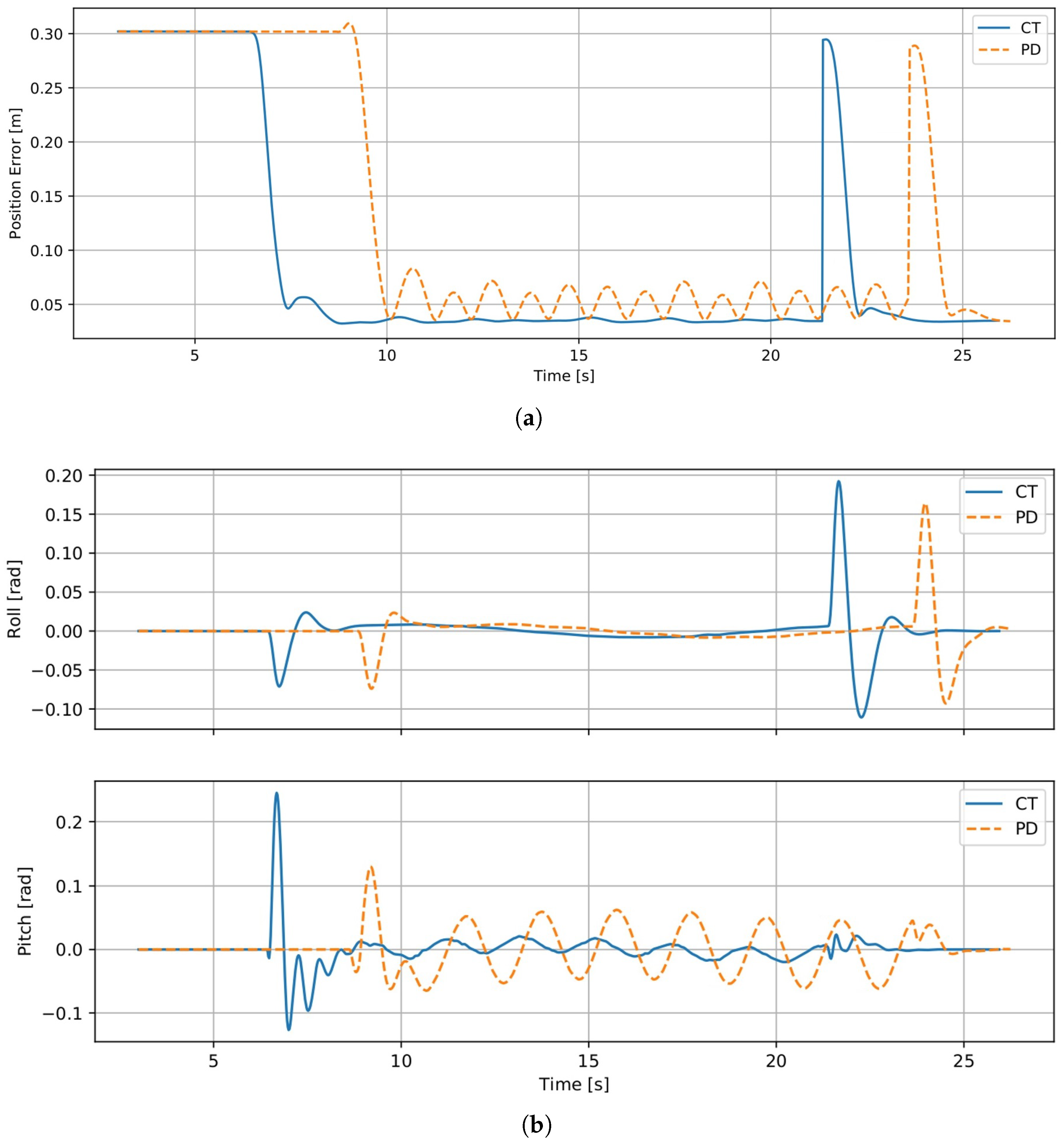
As shown in Figure 12, and specifically in Figure 12a, the CT controller demonstrates significantly faster convergence compared to the PD controller. Specifically, CT reaches steady state in approximately 3 s, whereas PD requires approximately 7 s and exhibits more oscillatory behavior. During steady-state operation (t ∈ [10, 20] s), the CT controller maintains a position tracking error of approximately 0.035 m, while the PD controller oscillates within the range of 0.04–0.08 m. At t ≈ 21 s, both controllers exhibit a transient spike corresponding to the termination of the circular trajectory and the subsequent return-to-origin maneuver (a 0.3 m step change in reference). Notably, the CT controller recovers more rapidly from this disturbance.

Figure 12b shows the drone orientation during Case 3. During steady-state tracking (t ∈ [10, 20] s), pitch deviations remain below 0.02 rad under CT control, whereas the PD controller exhibits sustained oscillations of approximately 0.05 rad at the arm trajectory frequency (0.5 Hz). These oscillations can be attributed to uncompensated inertial coupling between the manipulator motion and the quadrotor attitude dynamics. By incorporating cross-coupling terms derived from the mass and Coriolis matrices, the CT controller effectively compensates for these interactions and produces anticipatory attitude corrections. Both controllers display larger transient responses during the initial convergence (t ≈ 7 s) and at trajectory termination (t ≈ 21 s), with the CT controller recovering faster in both cases.

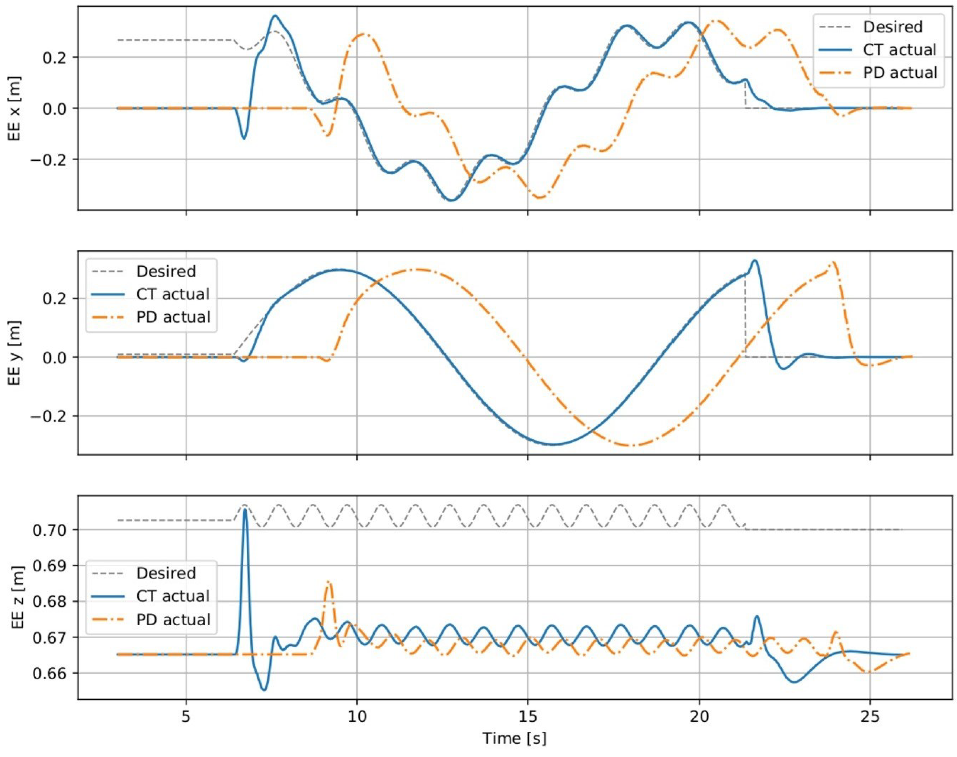
Figure 13, presents the end-effector position in the world frame for both controllers compared against the desired trajectory. In the x- and y-axes, the CT controller tracks the desired end-effector path with smaller deviations, whereas the PD controller exhibits larger deviations due to the slower convergence of the quadrotor base. During steady-state operation (t ∈ [10, 20] s), the CT end-effector position closely follows the desired reference in both horizontal axes, while the PD controller shows persistent offsets and delayed response.

In the vertical axis (z), both controllers maintain the end-effector near the desired height of approximately 0.70 m. However, the CT controller exhibits slightly larger oscillations (±0.005 m), attributable to its active coupling compensation that induces small pitch variations. Overall, the mean end-effector tracking error is reduced from 0.066 m (PD) to 0.036 m (CT), corresponding to a 46% improvement, as seen in Table 2.

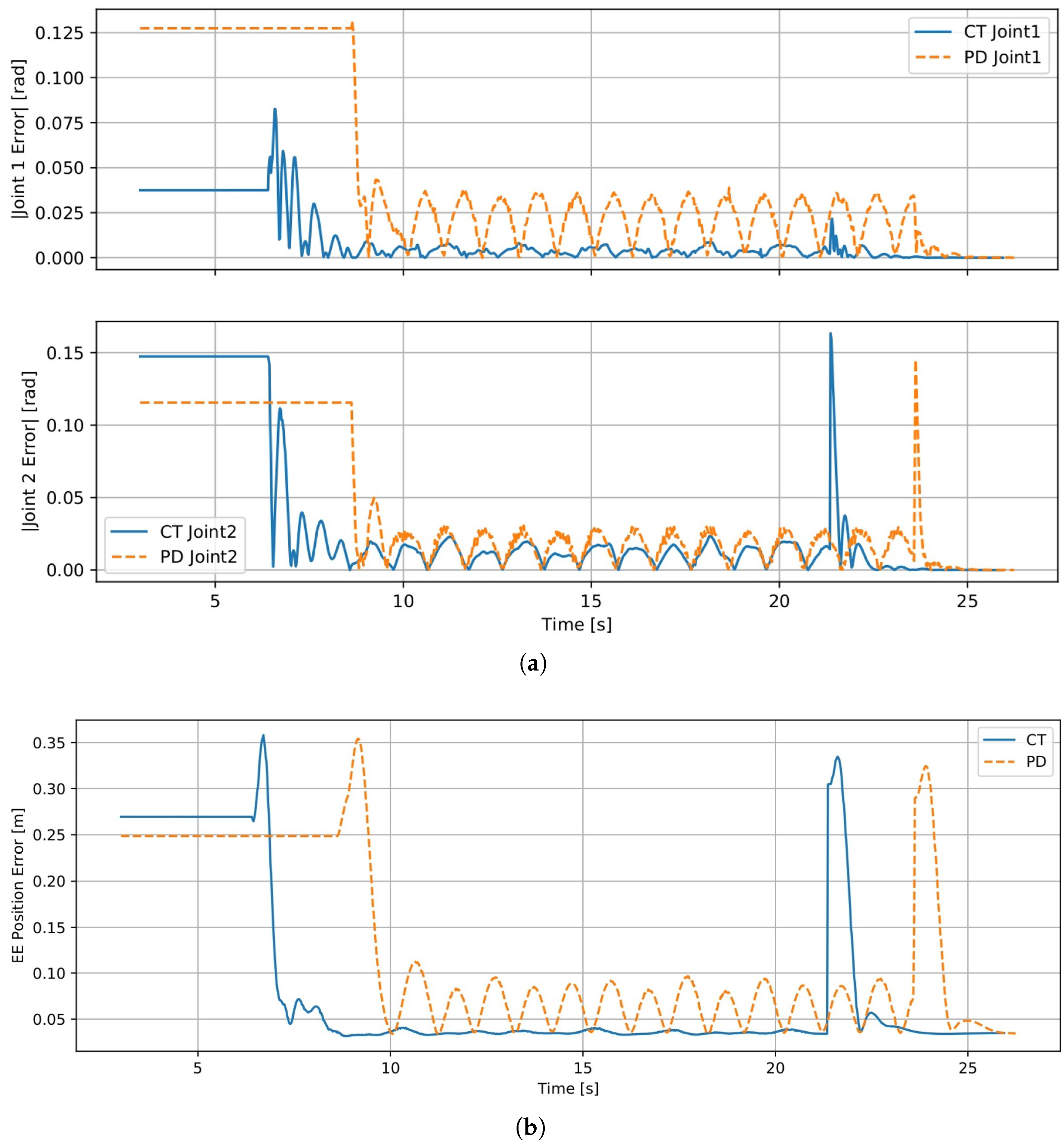
Figure 14a shows the absolute joint tracking error for both controllers. During steady-state operation (t ∈ [10, 20] s), the CT controller achieves Joint1 errors below 0.005 rad, compared to persistent oscillations of 0.02–0.04 rad for the PD controller. Joint2 exhibits similar behavior, with the CT controller maintaining errors of approximately 0.01 rad, whereas the PD controller oscillates within the range of 0.01–0.02 rad. The periodic oscillations observed in the PD joint errors at the trajectory frequency further confirm that the decoupled controller cannot adequately reject the coupling disturbances induced by the simultaneous quadrotor and arm motion. In contrast, the CT controller suppresses these disturbances through the feedforward acceleration term and the coupled mass matrix, which appropriately distributes the required torques.

Figure 14b presents the end-effector tracking error norm in the world frame. During steady-state operation (t ∈ [10, 20] s), the CT controller maintains an end-effector error of approximately 0.035 m, whereas the PD controller oscillates within the range of 0.04–0.10 m at the arm trajectory frequency.

The sustained oscillations observed in the PD error reflect the combined effect of uncompensated coupling on both the quadrotor base position and the arm joint tracking. In contrast, by accounting for the full coupled dynamics, the CT controller effectively suppresses these oscillations and achieves a 46% reduction in the mean end-effector tracking error (Table 2).

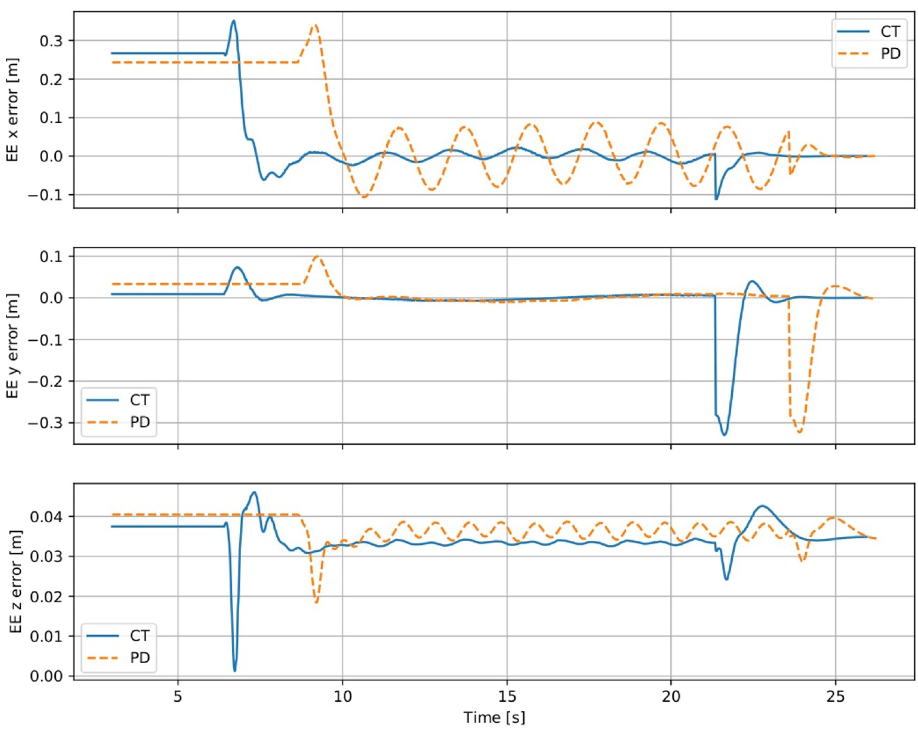
Figure 15 shows the end-effector tracking error by axis. The x and y components confirm that the PD controller exhibits persistent oscillations in the horizontal plane, with amplitudes ranging approximately from ±0.05 to ±0.10 m, whereas the CT controller maintains errors close to zero during steady-state operation. The z-axis error shows a consistent offset of approximately 0.03–0.04 m for both controllers, which can be attributed to a steady-state altitude tracking error caused by the additional weight of the manipulator on the quadrotor base.

The 46% reduction in mean end-effector tracking error (Table 2) reflects the combined effect of the time-varying coupling terms M_qη, C_qη, and C_ηq during simultaneous quadrotor lateral acceleration and arm motion. In this scenario, the inertial coupling terms are most significant, as the lateral acceleration of the quadrotor base generates time-varying reaction forces on the arm joints that the CT controller compensates through the off-diagonal mass matrix blocks, while the PD controller cannot account for these interactions.

Robustness to Wind Disturbance

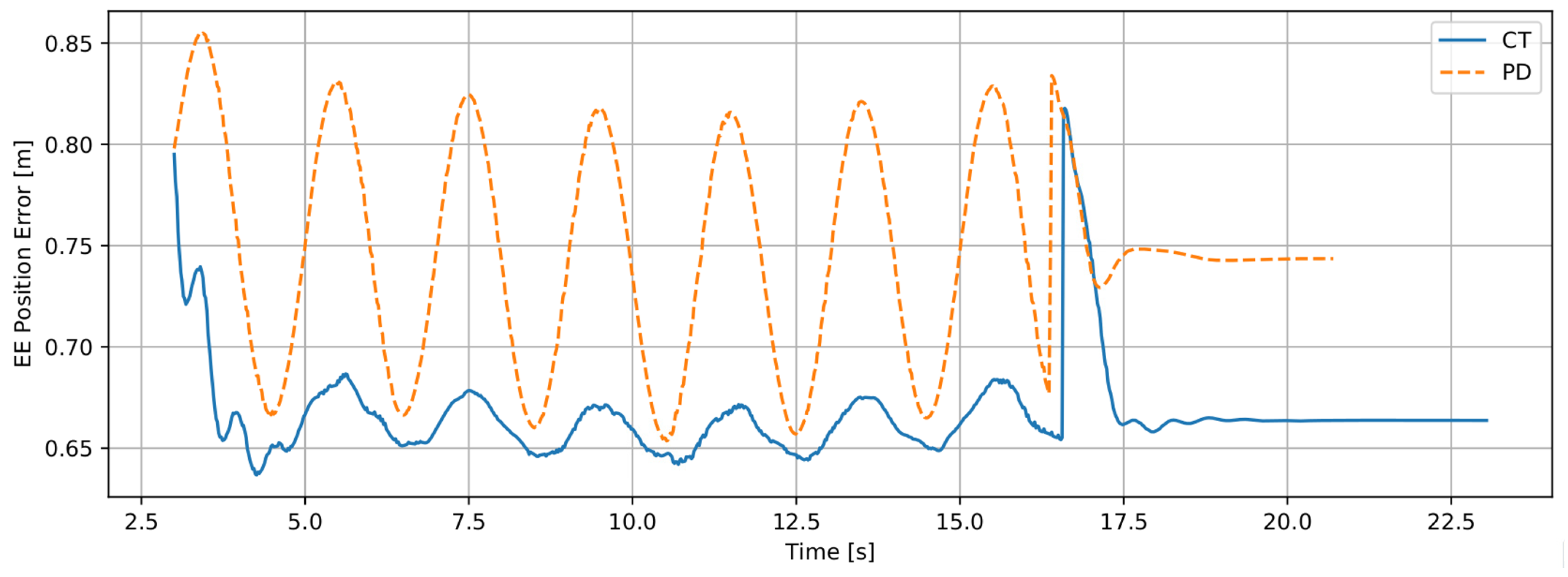
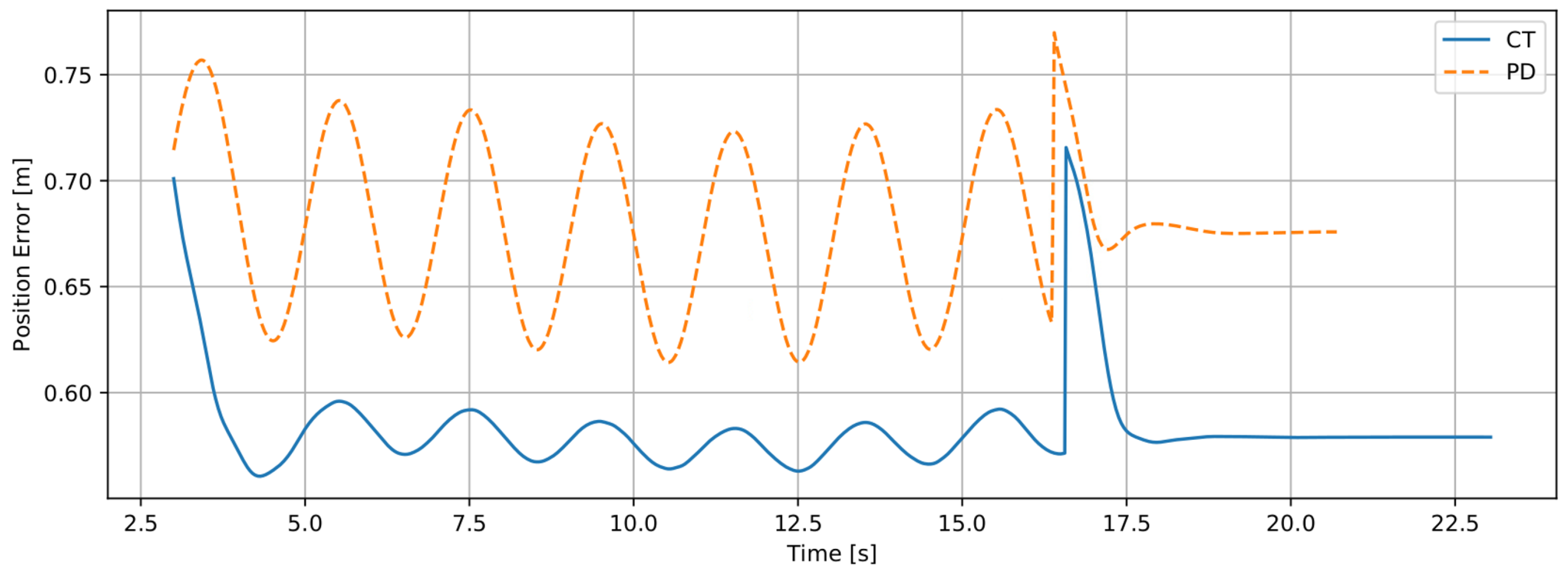
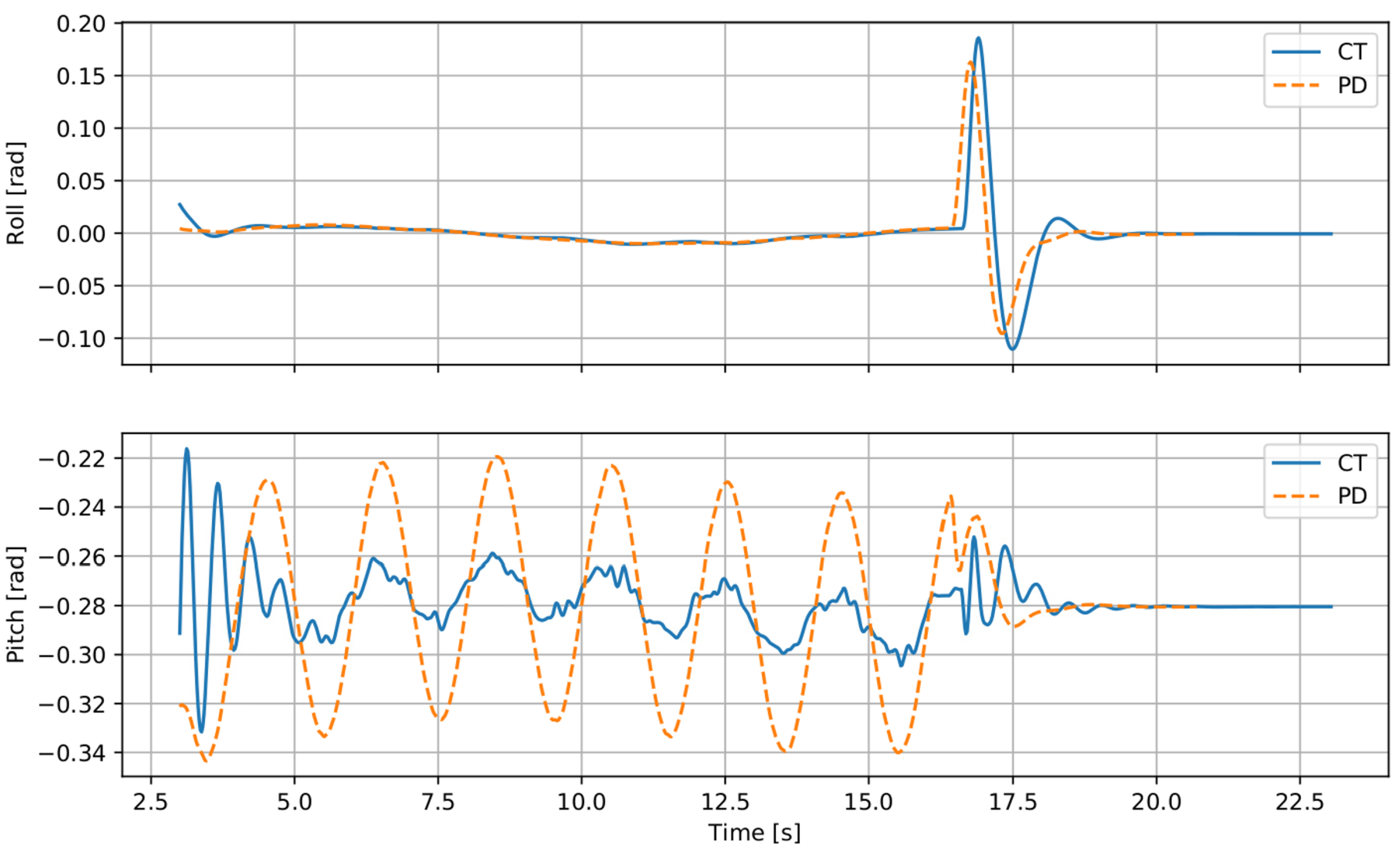
To assess robustness under persistent aerodynamic loading during the most demanding scenario, the Case 3 experiment (circular quadrotor trajectory with simultaneous sinusoidal arm motion) is repeated under a constant lateral wind of 2 m/s, applied along the world-frame x-axis using the RotorS Gazebo wind plugin, with identical conditions for both controllers. Neither controller incorporates a disturbance observer or integral action; consequently, both exhibit a steady-state position bias along the wind direction of approximately 0.58–0.67 m, attributable to the unrejected constant aerodynamic force. The comparison therefore evaluates relative disturbance rejection performance within this constrained operating regime, focusing on whether the coupled dynamics compensation of CT retains its advantage over the decoupled PD architecture under persistent wind. Metrics are computed over the steady-state window t ∈ [6, 16] s, excluding initial transients.

Figure 16 shows the quadrotor position tracking error norm during the Case 3 wind experiment. The CT controller reaches a stable steady-state level by t ≈ 6 s, with a small ripple (±0.01 m) at the arm trajectory frequency (0.5 Hz), consistent with the residual Coriolis coupling oscillation observed in the no-wind Case 3 scenario. The PD controller exhibits persistent oscillations of amplitude ±0.05–±0.07 m throughout the steady-state window, driven by the uncompensated interaction between the constant aerodynamic disturbance, the arm inertial coupling, and the quadrotor attitude loop. These oscillations are not present in the no-wind Case 3 results, confirming that wind disturbance amplifies the coupling-induced position errors that the CT controller suppresses through M_qη and C_qη but that the PD controller cannot compensate.

Figure 17 shows the quadrotor orientation during the Case 3 wind experiment. The steady-state pitch bias of −0.28 rad is common to both controllers and represents the geometric attitude required to partially resist the 2 m/s aerodynamic force through thrust vectoring in the absence of integral compensation. Within this biased operating point, CT suppresses the coupling-induced pitch oscillations to ±0.02 rad, compared to ±0.06 rad for PD—a threefold reduction in oscillation amplitude attributable to the C_qη Coriolis compensation block, which captures the periodic torques generated by simultaneous arm motion and quadrotor lateral acceleration. The CT transient pitch excursion at onset (0.647 rad) is larger than for PD (0.381 rad) due to the aggressive coupled inverse dynamics response to the simultaneous disturbances; both controllers reach comparable steady-state pitch levels by t ≈ 6 s.

Figure 18 shows the end-effector tracking error norm in the world frame, which is the primary performance metric for Case 3. During steady-state operation (t ∈ [6, 16] s), the CT controller maintains a near-constant EE error of approximately 0.66 m with minimal oscillation, while the PD controller exhibits persistent oscillations between 0.65 and 0.83 m at the arm trajectory frequency. The low-amplitude ripple observed in the CT end-effector error (±0.01 m) reflects the continuous coupled torque adjustments generated by the inverse dynamics model as it actively compensates the interaction between the constant aerodynamic bias, the circular quadrotor acceleration, and the arm joint motion—a characteristic of model-based coupled control that is distinct from instability. The oscillatory component in the PD EE error arises from the compounding of uncompensated coupling effects: the arm motion generates periodic inertial forces that disturb the quadrotor attitude, which in turn displaces the EE base position in the world frame, producing oscillations that the decoupled architecture cannot anticipate or suppress. The CT controller eliminates this oscillatory component through the time-varying coupling terms M_qη, C_qη, and C_ηq, consistent with the 46% EE error reduction reported for the no-wind Case 3 scenario (Table 2). Under 2 m/s constant wind, the relative improvement narrows to 11% mean and 17% peak EE error reduction, as the dominant error source shifts from coupling-induced oscillations to the unrejected aerodynamic bias—confirming that disturbance observer integration is the key next step for deployment under persistent wind conditions.

6. Conclusions and Discussion

This research presents a fully coupled hybrid geometric computed torque control approach for a quadrotor equipped with a 2-DOF planar robotic arm. Following the systematic E-L modeling methodology, the full 8-DOF dynamics equations capturing all coupling effects between the aerial vehicle and manipulator are derived. The proposed hybrid control architecture combines geometric control [14] for quadrotor translational and rotational motion with a low-level computed torque controller that explicitly exploits the complete coupled dynamics of the aerial–manipulator system. Case studies between the fully coupled and decoupled system demonstrate that the proposed hybrid controller achieves improved trajectory tracking performance in all test cases over decoupled control approaches. During quasi-static arm positioning (Case 1), the mean joint tracking error is reduced by 66% (from 0.057 rad to 0.019 rad), and the quadrotor position error by 52% (from 0.083 m to 0.040 m), at the expense of slightly larger transient pitch excursions due to the anticipatory coupling torques from the aggressive ramp transition. The integrated absolute error over the full run is reduced by 50% (from 2.33 to 1.17 m·s), confirming that the CT controller accumulates a lower total error despite the larger initial transient pitch excursions.

During continuous arm trajectory tracking in hover (Case 2), the pitch disturbance RMS is reduced by 82% (from 0.056 rad to 0.010 rad), and the quadrotor position error by 52% (from 0.065 m to 0.031 m). The PD controller requires 23.5 s to reach steady-state position accuracy, compared to 10 s for CT, indicating that the uncompensated coupling forces prevent the PD controller from settling within the standard experiment duration.

In the simultaneous quadrotor and arm trajectory tracking (Case 3) scenario, the coupled controller achieves a 46% reduction in mean end-effector tracking error (from 0.066 m to 0.036 m), a 61% reduction in mean joint tracking error, and a 74% reduction in pitch RMS, while maintaining comparable actuator effort (Table 2). These results validate the effectiveness of considering dynamic coupling in aerial manipulation systems and highlight the importance of accounting for inertial coupling, Coriolis, and centrifugal effects in the control design of aerial manipulation platforms, particularly during simultaneous base and manipulator motion. The CT controller reaches steady state at 10 s compared to 24.5 s for PD, a 2.4× improvement in convergence speed attributable to the anticipatory coupling compensation in M_qη.

Additional wind disturbance experiments on Case 2 (2 m/s lateral gust, 3 s) and Case 3 (2 m/s constant lateral wind) confirm that the CT controller retains its advantage over the decoupled PD baseline under aerodynamic disturbances, achieving up to 23% reduction in position error and 17% reduction in end-effector error. This relative improvement narrows under constant wind as the unrejected aerodynamic bias dominates over the coupling-induced oscillations that CT suppresses, motivating disturbance observer integration and adaptive compensation as primary directions for future work.

Future research directions include the integration of adaptive control terms to handle system uncertainties, experimental validation of the proposed work, and extension to cooperative manipulation tasks, building upon our previous research [20,21,22]. A dedicated parameter identification study will further support the hardware implementation of the proposed CT controller, which relies on accurate system model knowledge. Regarding the small-roll-and-pitch assumption (${\mathbf{R}}_t\approx \mathbb{I}$) used in the joint gravity evaluation (Section 3.6), the attitude ranges observed across all simulation cases confirm its validity during steady-state operation. Roll remains below ±0.001 rad in Cases 1 and 2 and below ±0.010 rad in Case 3. Pitch remains below ±0.03 rad during steady state across all cases, with larger transient excursions of up to ±0.25 rad occurring only during the initial arm motion phase. At these steady-state attitude ranges and given the lightweight manipulator links (m₁ = m₂ = 0.04 kg), the resulting approximation error in joint gravity torques is bounded by approximately 0.004 Nm, which is negligible compared to the commanded torque range of 0.03–0.05 Nm RMS. Full gravity compensation without this assumption is planned for the hardware implementation. These developments will enhance the robustness and practical applicability of the proposed hybrid control framework for real-world aerial manipulation scenarios.

References

1. Almurib, H.; Nathan, P.; Kumar, T. Control and path planning of quadrotor aerial vehicles for search and rescue. In Proceedings of the SICE Annual Conference, Tokyo, Japan, 13–18 September 2011; pp. 700–705. [Google Scholar]
2. Wu, Y.; Wu, S.; Hu, X. Multi-constrained cooperative path planning of multiple drones for persistent surveillance in urban environments. Complex Intell. Syst. 2021, 7, 1633–1647. [Google Scholar] [CrossRef] [Scilit]
3. Ruggiero, F.; Lippiello, V.; Ollero, A. Aerial Manipulation: A Literature Review. IEEE Robot. Autom. Lett. 2018, 3, 1957–1964. [Google Scholar] [CrossRef] [Scilit]
4. Aerial Robotics Cooperative Assembly System. EU Research. 2011–2015. Available online: https://cordis.europa.eu/project/id/287617 (accessed on 7 April 2026).
5. Korpela, C.; Orsag, M.; Danko, T.; Oh, P. Insertion tasks using an aerial manipulator. In Proceedings of the IEEE International Conference on Technologies for Practical Robot Applications (TePRA), Woburn, MA, USA, 14–15 April 2014. [Google Scholar]
6. Khamseh, H.B.; Janabi-Sharifi, F.; Abdessameud, A. Aerial manipulation—A literature survey. Robot. Auton. Syst. 2018, 107, 221–235. [Google Scholar] [CrossRef] [Scilit]
7. Barakou, S.C.; Tzafestas, C.S.; Valavanis, K.P. Control Strategies for Real-Time Aerial Manipulation with Multi-Dof Arms: A Survey. In Proceedings of the 2025 International Conference on Unmanned Aircraft Systems (ICUAS), Charlotte, NC, USA, 14–17 May 2025. [Google Scholar]
8. Li, Z.; Li, H.; Xu, Q.; Yu, X.; Basin, M.V. Coupling Disturbance Modeling and Compensation for Aerial Manipulator in Highly Dynamic Motion. IEEE Trans. Cybern. 2024, 55, 124–135. [Google Scholar] [CrossRef] [Scilit] [PubMed]
9. Wu, Y.; Zhou, Z.; Wei, M.; Cheng, H. Robust and Energy-Efficient Control for Multi-task Aerial Manipulation with Automatic Arm-switching. In Proceedings of the IEEE International Conference on Robotics and Automation (ICRA), Yokohama, Japan, 13–17 May 2024. [Google Scholar]
10. Lee, D.; Seo, H.; Kim, D.; Kim, H.J. Aerial Manipulation using Model Predictive Control for Opening a Hinged Door. In Proceedings of the IEEE International Conference on Robotics and Automation (ICRA), Paris, France, 31 May–31 August 2020. [Google Scholar]
11. Kim, S.; Choi, S.; Kim, H.J. Aerial Manipulation Using a Quadrotor with a Two DOF Robotic Arm. In Proceedings of the IEEE/RSJ International Conference on Intelligent Robots and Systems (IROS), Tokyo, Japan, 3–7 November 2013. [Google Scholar]
12. Guo, P.; Xu, K.; Deng, H.; Liu, H.; Ding, X. Modeling and control for aerial manipulation based on center of inertia on SE(3). Nonlinear Dyn. 2023, 111, 369–389. [Google Scholar] [CrossRef] [Scilit]
13. Bulut, N.; Turgut, A.; Arikan, K.B. Computed Torque Control of an Aerial Manipulation System with a Quadrotor and a 2-DOF Robotic Arm. In Proceedings of the 16th International Conference on Informatics in Control, Automation and Robotics, Prague, Czech Republic, 29–31 July 2019. [Google Scholar]
14. Furrer, F.; Burri, M.; Achtelik, M.; Siegwart, R. RotorS—A Modular Gazebo MAV Simulator Framework. In Robot Operating System (ROS); Springer: Cham, Switzerland, 2016; Volume 1, pp. 595–625. [Google Scholar]
15. Siciliano, B.; Sciavicco, L.; Villani, L.; Oriolo, G. Robotics: Modelling, Planning and Control; Springer: London, UK, 2009. [Google Scholar]
16. Spong, M.W.; Hutchinson, S.; Vidyasagar, M. Robot Modeling and Control; John Wiley & Sons, Inc.: Hoboken, NJ, USA, 2005. [Google Scholar]
17. Murray, R.M.; Li, Z.; Sastry, S.S. A Mathematical Introduction to Robotic Manipulation; CRC Press: Boca Raton, FL, USA, 1994. [Google Scholar]
18. Featherstone, R. Rigid Body Dynamics Algorithms; Springer: New York, NY, USA, 2008. [Google Scholar]
19. Lee, T.; McClamroch, M.L.N.H. Geometric tracking control of a quadrotor UAV on SE(3). In Proceedings of the 49th IEEE Conference on Decision and Control (CDC), Atlanta, GA, USA, 15–17 December 2010. [Google Scholar]
20. Barakou, S.C.; Tzafestas, C.S.; Valavanis, K.P. Real-Time Applicable Cooperative Aerial Manipulation: A Survey. In Proceedings of the International Conference on Unmanned Aircraft Systems (ICUAS), Warsaw, Poland, 6–9 June 2023. [Google Scholar]
21. Barakou, S.C.; Tzafestas, C.S.; Valavanis, K.P. A Survey of Modeling and Control Approaches for Cooperative Aerial Manipulation. In Proceedings of the International Conference on Unmanned Aircraft Systems (ICUAS), Chania-Crete, Greece, 4–7 June 2024. [Google Scholar]
22. Barakou, S.C.; Tzafestas, C.S.; Valavanis, K.P. A Review of Real-Time Implementable Cooperative Aerial Manipulation Systems. Drones 2024, 8, 196. [Google Scholar] [CrossRef] [Scilit]
Figure 2. Control architecture.
Drones 10 00274 g002
Figure 3. Quadrotor roll and pitch during Case 1 (hovering with arm ramp). CT exhibits larger transient pitch excursions (±0.13 rad) due to anticipatory coupling compensation via M, while PD shows smaller but sustained pitch deviations. Both controllers maintain near-zero roll, consistent with the planar arm geometry.
Drones 10 00274 g003
Figure 4. Arm ramp experiment. (a) Joint tracking error during Case 1. CT achieves near-zero steady-state error between transitions while PD exhibits prolonged settling of approximately 5 s per set point. (b) Joint angles (desired vs. actual) during Case 1. CT tracks the ±0.3 rad ramp within ≈2 s while PD requires ≈5 s to converge to each set point due to uncompensated inertial coupling.
Drones 10 00274 g004
Figure 5. Quadrotor position tracking error norm during Case 1. CT shows brief transient peaks of 0.07–0.09 m returning to baseline within 2 s, while PD accumulates a sustained error of 0.13–0.14 m when the arm is held at ±0.3 rad due to the uncompensated shift in the system center of mass.
Drones 10 00274 g005
Figure 6. Quadrotor roll and pitch during Case 2 (hovering with sinusoidal arm trajectory at 0.5 Hz). CT maintains pitch below 0.02 rad while PD exhibits sustained oscillations of ±0.07 rad at arm trajectory frequency, attributed to uncompensated Coriolis coupling block C.
Drones 10 00274 g006
Figure 7. Arm trajectory experiment. (a) Quadrotor position tracking error norm during Case 2. CT maintains ≈0.031 m steady-state error while PD oscillates between 0.04–0.09 m at arm trajectory frequency. (b) Quadrotor position tracking error per axis during Case 2 with CT and PD overlaid. PD oscillations are concentrated along x-axis, consistent with pitch–translation coupling from planar arm motion.
Drones 10 00274 g007
Figure 8. Arm joint tracking errors during Case 2. CT maintains Joint 1 error below 0.02 rad while PD exhibits persistent oscillations of 0.04–0.06 rad due to uncompensated Coriolis coupling at 0.5 Hz arm trajectory frequency.
Drones 10 00274 g008
Figure 9. Quadrotor pitch during the Case 2 wind disturbance experiment (2 m/s lateral gust, 3 s duration, injected at t = 7.5 s). CT exhibits a peak of −0.32 rad resolving by t ≈ 11 s. PD reaches −0.40 rad and sustains oscillations for ≈5 s post-gust. Post-gust pitch RMS: CT 0.121 rad vs. PD 0.138 rad.
Drones 10 00274 g009
Figure 10. Quadrotor position tracking error per axis during the Case 2 wind disturbance experiment. The x-axis (gust direction) shows CT peaking at 0.55 m and PD at 0.71 m. Over t ∈ [5, 20] s, CT achieves 23% reduction in mean position error (0.13 m vs. 0.17 m) and 27% reduction in IAE (2.04 vs. 2.80 m·s). The y- and z-axes remain comparable between both controllers.
Drones 10 00274 g010
Figure 11. Arm joint tracking errors during the Case 2 wind disturbance experiment. Joint 1 (top): CT stays below 0.03 rad after startup transient; PD oscillates 0.02–0.11 rad throughout. Joint 2 (bottom): CT exhibits marginally larger oscillations than PD, attributable to pitch corrections propagating through M—an inherent trade-off of the coupled architecture. IAE joint: CT 1.14 rad·s vs. PD 1.34 rad·s.
Drones 10 00274 g011
Figure 12. Aerial manipulation experiment. (a) Quadrotor position tracking error during Case 3 (circular trajectory with simultaneous arm motion). CT reaches steady state in ≈3 s while PD requires ≈7 s. Both controllers show transient spike at t ≈ 21 s, corresponding to trajectory termination. (b) Quadrotor orientation during Case 3. CT maintains pitch below 0.02 rad during steady state while PD exhibits sustained oscillations of ≈0.05 rad at arm trajectory frequency (0.5 Hz).
Drones 10 00274 g012
Figure 13. End-effector position in the world frame (desired vs. actual) during Case 3. CT tracks the desired trajectory with smaller deviations in all axes, achieving a 46% reduction in mean end-effector error compared to PD (0.036 m vs. 0.066 m).
Drones 10 00274 g013
Figure 14. Aerial manipulation experiment. (a) Arm joint tracking errors during Case 3. CT achieves Joint 1 errors below 0.005 rad during steady state compared to persistent oscillations of 0.02–0.04 rad for PD. (b) End-effector tracking error norm in world frame during Case 3. CT maintains ≈0.035 m while PD oscillates between 0.04–0.10 m at arm trajectory frequency.
Drones 10 00274 g014
Figure 15. End-effector tracking error per axis during Case 3. PD exhibits persistent oscillations of ±0.05–±0.10 m in the horizontal plane (x, y), while CT maintains near-zero errors during steady-state operation. The z-axis offset of ≈0.03–0.04 m is present in both controllers and is attributed to the steady-state altitude error induced by the manipulator weight.
Drones 10 00274 g015
Figure 16. Quadrotor position tracking error norm during Case 3 under 2 m/s constant lateral wind (t ∈ [6, 16] s). CT maintains a steady mean error of 0.577 m with ±0.01 m ripple, while PD oscillates between 0.62 and 0.73 m. CT achieves a 14% reduction in mean and 19% reduction in peak position error.
Drones 10 00274 g016
Figure 17. Quadrotor orientation during Case 3 under 2 m/s constant lateral wind (t ∈ [6, 16] s). Both controllers share a steady-state pitch bias of −0.28 rad from thrust vectoring against the wind; CT suppresses coupling-induced pitch oscillations to ±0.02 rad vs. ±0.06 rad for PD.
Drones 10 00274 g017
Figure 18. End-effector tracking error norm during Case 3 under 2 m/s constant lateral wind (t ∈ [6, 16] s). CT maintains 0.661 m mean EE error with ±0.01 m oscillation, while PD oscillates between 0.65 and 0.83 m. CT achieves 11% reduction in mean EE error (0.661 m vs. 0.741 m) and 17% reduction in peak (0.684 m vs. 0.829 m).
Drones 10 00274 g018