Optimal Path Planning for High-Altitude Low-Speed Aerostats Under Complex Constraints

Highlights

What are the main findings?

• Proposes a Markov decision process (MDP)-based path planning method that effectively handles uncertainties in forecasted wind fields for high-altitude low-speed aerostats.
• Enables optimal 2D and 3D global path planning and quantitative regional reachability analysis under complex constraints like limited propulsion and flight time.

What are the implications of the main findings?

• Provides a practical theoretical basis and strategic guidance for the rapid emergency deployment and operational planning of aerostats.
• Offers quantitative assessment for selecting optimal launch points and formulating flight strategies by evaluating the impact of wind resistance on reachability.

Abstract

High-altitude low-speed aerostats are ideal unmanned platforms for communication coverage, remote sensing, environmental monitoring, aviation support, and other applications. To address practical operational needs such as rapid emergency deployment, this paper proposes a path planning method for low-speed aerostats based on the Markov decision process (MDP). The method is optimized to minimize deployment time while accounting for discrepancies between forecasted and actual wind fields. An uncertain wind field model is established to incorporate wind-related uncertainties into the MDP framework, with key parameters—including the state space, action set, immediate reward, and transition probability—designed accordingly. A mathematical model is formulated to address the global path planning problem under complex constraints, such as horizontal wind resistance capability, altitude control capacity, and flight time requirements. Simulation results demonstrate that the proposed method enables aerostats to achieve optimal 2D and 3D path planning under complex constraints. Furthermore, regional reachability is quantitatively analyzed, providing technical support for the rapid deployment of aerostats to target areas in practical applications. The core innovations of this work lie in the integration of a probabilistic wind uncertainty model with a constraint-aware MDP framework, enabling optimal 3D path planning and quantitative reachability analysis for high-altitude low-speed aerostats.

1. Introduction

High-altitude low-speed aerostats are unmanned buoyant vehicles that have emerged as transformative platforms for persistent Earth observation, communication relay, and environmental monitoring, owing to their exceptional endurance, wide coverage, and cost-effectiveness [1]. Realizing their full operational potential hinges on a critical capability: reliable and time-efficient path planning from a launch site to a distant target area [2].

The path planning problem for aerostats is uniquely challenging and distinct from that of highly maneuverable unmanned aerial vehicles (UAVs). Aerostats are characterized by their low dynamics, large size, and fundamental coupling with atmospheric winds, making their trajectories predominantly wind-driven [3]. Crucially, their operational envelope is bounded by stringent physical constraints. These include severely limited on-board propulsion for wind counteraction, a finite altitude adjustment range that is typically managed through ballonet systems or gas venting [4,5], and the overarching scarcity of electrical energy for both propulsion and station-keeping [6]. Therefore, the core problem transcends conventional obstacle avoidance; it requires computing a time-optimal trajectory under probabilistic wind uncertainty while strictly adhering to these platform-specific actuation and energy limits.

Classical path planning methods (e.g., graph-search, potential fields) often lack explicit mechanisms to handle environmental uncertainty and hard physical constraints [7,8]. The Markov decision process (MDP) provides a rigorous, model-based framework for sequential decision-making under uncertainty, with proven applications in related domains like planetary balloon navigation [9]. Concurrently, the field is being advanced by data-driven paradigms. Deep reinforcement learning (DRL) has shown remarkable success in learning complex control policies, as evidenced by the recent work on stratospheric airship planning in complex environments [10]. Furthermore, the integration of large AI models is envisioned to orchestrate future intelligent aerial ecosystems [11]. However, while being promising in their adaptability, these data-intensive methods often face significant challenges in guaranteeing hard constraint satisfaction and ensuring operational safety—paramount concerns for aerostat applications with scarce real-world flight data [12].

To bridge this gap, this paper proposes a novel, model-based MDP framework that is explicitly designed for aerostat path planning. Our approach integrates a probabilistic wind uncertainty model and encodes the key physical constraints of aerostats directly into the MDP’s core structure. This design ensures that all generated paths are physically feasible by construction, offering a high degree of interpretability and safety assurance. The primary contributions of this work are:

• An integrated MDP formulation that jointly addresses probabilistic wind fields and the complex physical constraints that are inherent to high-altitude low-speed aerostats.
• A 3D optimal path planning algorithm that enables strategic altitude-layer selection to exploit wind shear, coupled with a quantitative regional reachability analysis tool for mission pre-assessment.
• Comprehensive simulation studies validating the method’s efficacy in generating time-optimal 2D/3D paths under uncertainty and constraints, demonstrating its practical utility.

2. Related Work

2.1. Planning Characteristics and Physical Constraints of Aerostats

Path planning requirements vary fundamentally across robotic platforms.

Table 1. Comparison of path planning characteristics.

Platform	Core Characteristics	Primary Env. Factor	Key Physical and Operational Constraints
High-Altitude Aerostat	Low dynamics, large size, wind-coupled	Wind field	Limited thrust [15], bounded altitude range [4,5], scarce on-board energy [6], coupled dynamics [16]
UAV	High maneuverability	Obstacles, other agents	Dynamics, sensor/comm. range, battery life
AUV	High maneuverability	Obstacles, other agents	Dynamics, sensor/comm. range, battery life

contrasts aerostats with unmanned aerial vehicles (UAVs) and autonomous underwater vehicles (AUVs). While UAV planning focuses on obstacle avoidance [13] and AUVs on current utilization [14], aerostat planning is dominated by wind interaction and hard system limits [3].

Aerostat-specific constraints are well-documented in the literature: a primary challenge is altitude control, which is often managed via ballonets. Research has modeled the dynamics of such systems and their energy consumption, highlighting the trade-offs involved in maintaining altitude [4,5]. Furthermore, their propulsion capability is inherently limited. Studies on multi-vectored thrust aerostats detail the constraints of actuator positioning, slew rates, and saturation, which directly dictate the feasible set of horizontal forces [15]. The coupled dynamics between the envelope and the suspended gondola also influence stability and controllability, imposing further restrictions on feasible trajectories [16]. These works collectively underscore that any practical path planner must treat these physical limits as first-order design constraints, not merely as post hoc feasibility checks.

2.2. Evolution of Path Planning Methodologies

Classical and optimization-based methods: Deterministic algorithms (A*, Dijkstra) lack mechanisms for uncertainty [7]. Sampling-based methods (RRTs) offer no optimality guarantees [17]. The artificial potential field method is prone to local minima [8]. Population-based optimizers (genetic algorithms) are often too computationally intensive for the sequential decision-making required in dynamic wind fields [18].

Learning-based and data-driven methods: Reinforcement learning (RL) and DRL learn policies through interaction [19]. For stratospheric vehicles, recent work by Wang et al. [10] represents a state-of-the-art DRL-based path planner. The emerging paradigm of large AI models, as discussed by Li et al. [11], envisions high-level orchestration of aerial networks. While powerful for adaptation, these methods face inherent challenges in sample efficiency, safety verification, and hard constraint satisfaction—critical limitations for safety-sensitive, data-scarce aerostat operations [12].

2.3. Markov Decision Processes in Stochastic Planning for Constrained Systems

The MDP framework provides a principled foundation for planning under uncertainty [20]. In aerospace, seminal work by Wolf et al. (2010) applied MDPs to global path planning for balloons under strong, uncertain winds [9]. The key strength of the model-based MDP approach in the context of constrained systems like aerostats is its ability to explicitly encode physical limits into the model. This allows for the direct computation of policies that are feasible and optimal within the defined constraint set, offering transparency and rigorous safety guarantees that are complementary to data-driven methods.

2.4. Identified Research Gap and Our Contribution

Synthesizing the literature reveals a clear gap. Advanced data-driven methods (e.g., [10]) excel in adaptability but face hurdles in guaranteeing hard physical constraints derived from aerostat design (e.g., [4,5,15]). Conversely, while model-based MDP methods [9] provide robustness and interpretability, their application has not been fully extended to solve the integrated 3D path planning problem for aerostats, where altitude selection and thrust limits are core, optimized strategic actions.

This work bridges this gap. We extend the rigorous, model-based MDP methodology to develop a novel 3D planning framework that explicitly incorporates the dominant physical constraints of aerostats. By integrating insights from aerostat dynamics and the control literature [4,5,15,16] into our MDP formulation, we ensure that feasibility and safety are inherent properties of the solution. Our approach is complementary to DRL; it provides a verifiable, constraint-guaranteed, and data-efficient solution for the critical mission planning phase of aerostat operations.

3. Models

3.1. Overview of the MDP

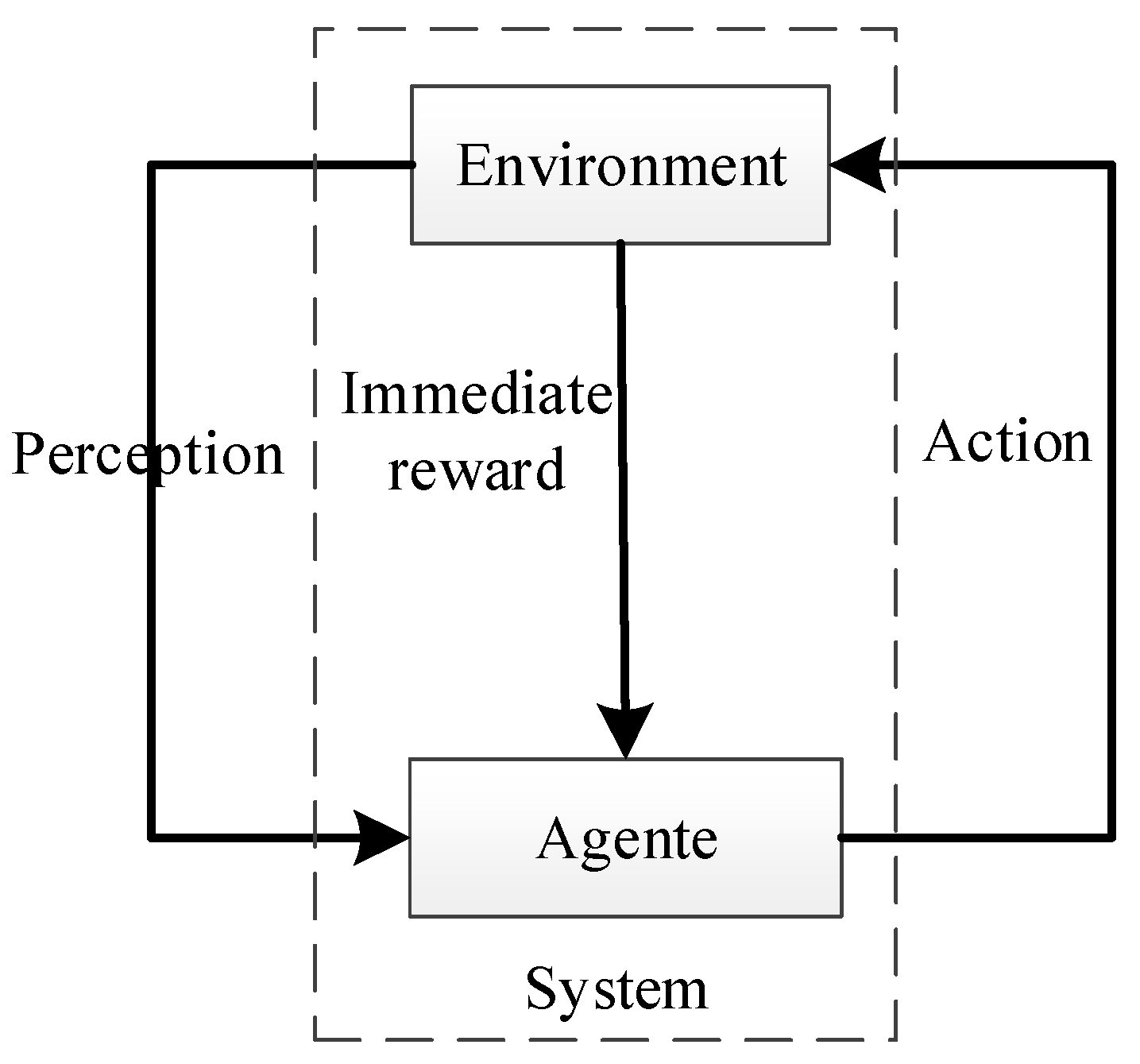
The MDP model is a framework that describes the interaction between an agent and its external environment, as shown in Figure 1. The system states encompass both the agent’s own state and the environmental state. The agent’s perception of the external environment serves as input, allowing it to execute actions from the action set, which alters the states of both the agent and the environment. During state transitions, the agent receives immediate rewards. Actions are selected to maximize the immediate reward over time. The core problem of the MDP model is to determine the optimal policy—i.e., the sequence of actions to choose at each decision point—such that the agent maximizes the immediate reward over its entire operational trajectory while achieving a predefined objective [21].

The MDP model is formally represented by $M=(S,A,R,P,\gamma )$. $S$ denotes the set of system states, encompassing both the agent’s internal state and environmental conditions. $A$ represents the set of all actions that are available (horizontal/vertical actuation) to the agent. $R_a(s_i,s_j)$ specifies the immediate reward received when the agent transitions from state $s_i$ to state $s_j$. $P_a(s_i,s_j)$ defines the transition probability of moving to state $s_j$ from state $s_i$ under action $a$. $\gamma$ represents the discount factor, the range of value is $[0,1)$, the greater, the greater the impact of subsequent rewards on the current reward.

When modeling sequential decision problems with MDP, the solution to the problem is a policy of $\pi :S\to A$, which is a mapping from the state space $S$ to the set of actions $A$. The solving process of MDP can be expressed as the problem of solving the optimal strategy ${\pi }^{\ast }$ that maximizes the cumulative reward. The cumulative reward is formally captured by the state-value function $V^{\pi }(s)$, representing the expected sum of discounted rewards from state $s$under policy $\pi$. This is expressed mathematically as follows:

$$V^{\pi }(s)=E^{\pi }({\displaystyle \sum _{t=0}^{\infty }{\gamma }^t{R}_t\left|s_0=s\right.}) ,$$

(1)

where $s_0$ is the start state, $R_t$ means the immediate reward at time $t$, and $\gamma$ means the discount factor.

The optimal value of $V^{\pi }(s)$ can be calculated in any state which satisfies $V^{{\pi }^{\ast }}(s)\ge V^{\pi }(s)$. The search strategy adopts the dynamic programming method, which corresponds to the start state and expands. The formula is the Bellman Equation, which is a necessary and sufficient condition for making the state value function optimal:

$$V^{{\pi }^{\ast }}(s_i)=\underset{a}{\max }(R_a(s_i,s_j)+\gamma {\displaystyle \sum _{s\prime \in S}{P}_a^{\pi (s)}}(s_i,s_j)V^{{\pi }^{\ast }}(s_j)),$$

(2)

The strategy corresponding to the optimal state value function is the optimal strategy, which can be expressed as follows:

$${\pi }^{\ast }(s_i)=\arg \underset{a}{\max }(R_a(s_i,s_j)+\gamma {\displaystyle \sum _{s\prime \in S}{P}_a^{\pi (s)}}(s_i,s_j)V^{{\pi }^{\ast }}(s_j)),$$

(3)

Common methods for solving optimal policies include policy iteration and value iteration [19]. The policy iteration method requires waiting for the value of each state to converge before performing a policy improvement step. This process is iteratively repeated until the policy itself converges. In contrast, the value iteration method updates the state-value function once and then immediately performs a policy improvement step. This cycle of updating the state-value function and improving the policy is repeated until the state-value function ultimately converges. In this paper, the value iteration method is adopted to solve for the optimal state-value function.

3.2. Modeling Wind Uncertainty

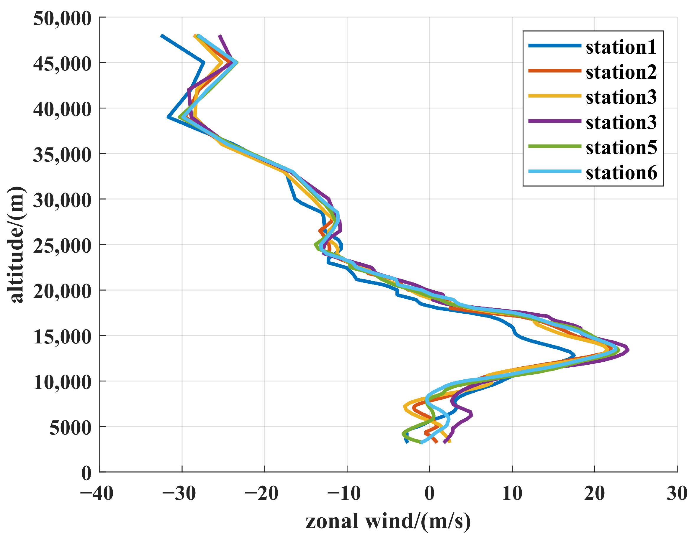
The actual wind vector varies in space and time. However, wind field characteristics above and below the quasi-zero-wind layer exhibit minimal temporal variation. Therefore, the spatial wind distribution must be prioritized in aerostat path planning. This study utilizes data from six meteorological stations, with Figure 2 illustrating the vertical profiles of east–west wind components at these sites. During high-altitude low-speed aerostats operations, wind information (velocity and direction at specific altitudes) used for navigation is derived from meteorological prediction models. However, discrepancies between real wind conditions and model predictions introduce uncertainties in path planning, necessitating the development of an uncertain wind field model [9].

3.2.1. Spatial Distribution of Wind Fields

We first use data from several meteorological stations to describe the 3D spatial distribution of wind fields. The steps are as follows:

1. Altitude interpolation

Meteorological stations can provide wind field data (velocity and direction) at specific altitudes. Linear interpolation is employed, using known altitude measurements to estimate wind conditions at goal altitudes, as demonstrated in Equation (4):

$$H={\displaystyle \frac{(H-H_2)}{(H_1-H_2)}}{H}_2-{\displaystyle \frac{(H-H_1)}{(H_2-H_1)}}{H}_1,$$

(4)

where $H_1$ and $H_2$ are known altitudes with wind data at station 1 and station 2, and $H$ is the target altitude.

2. 2D spatial distribution of wind fields

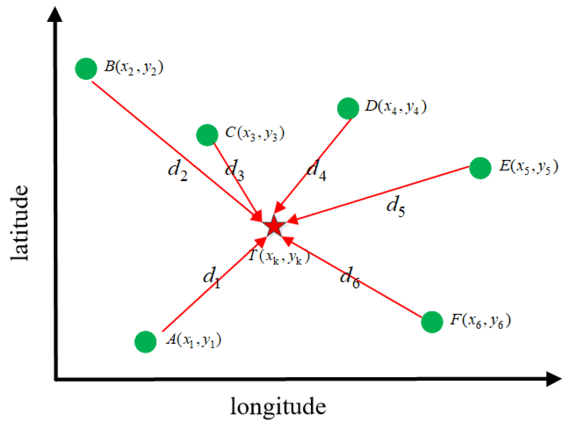
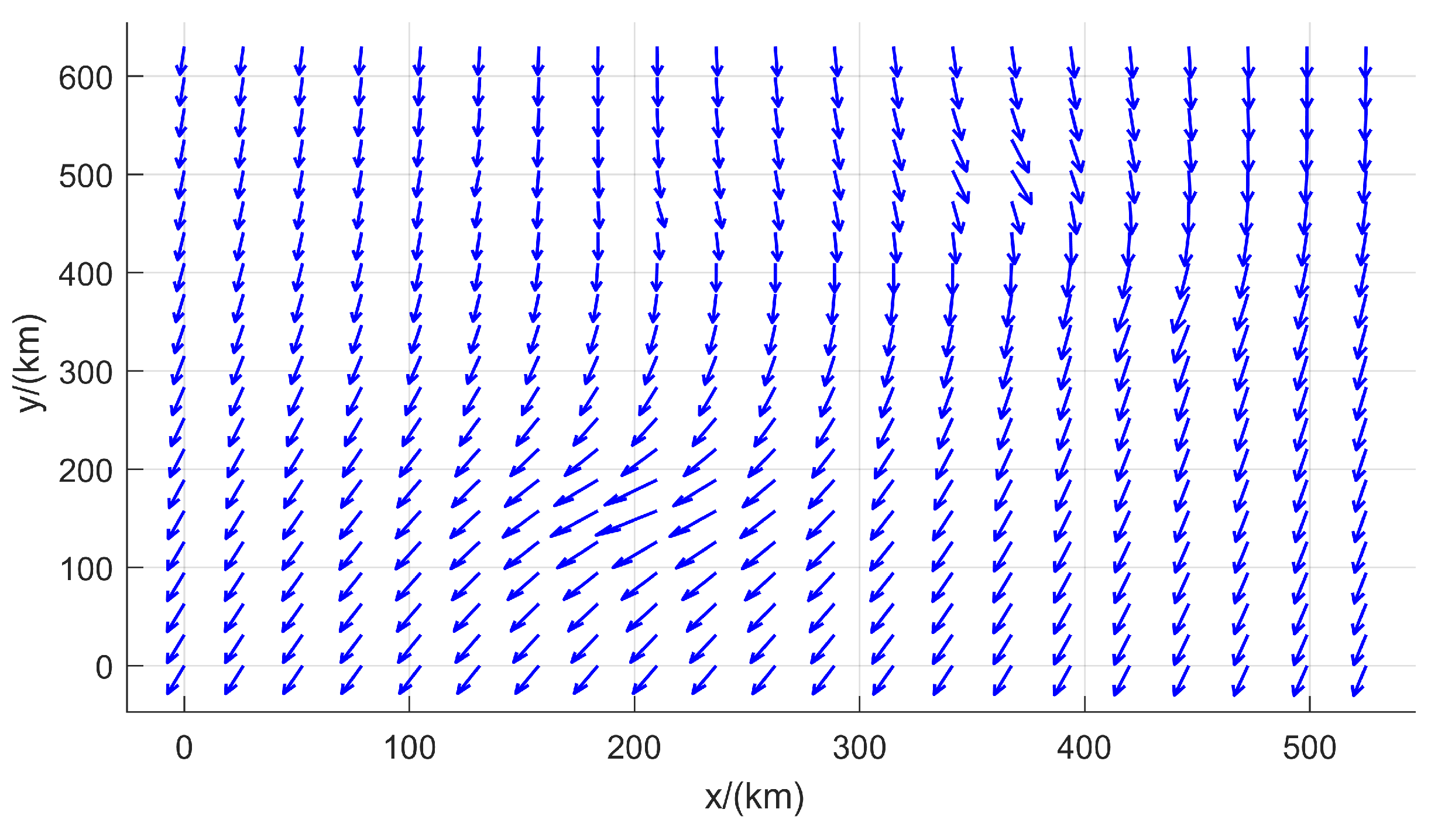
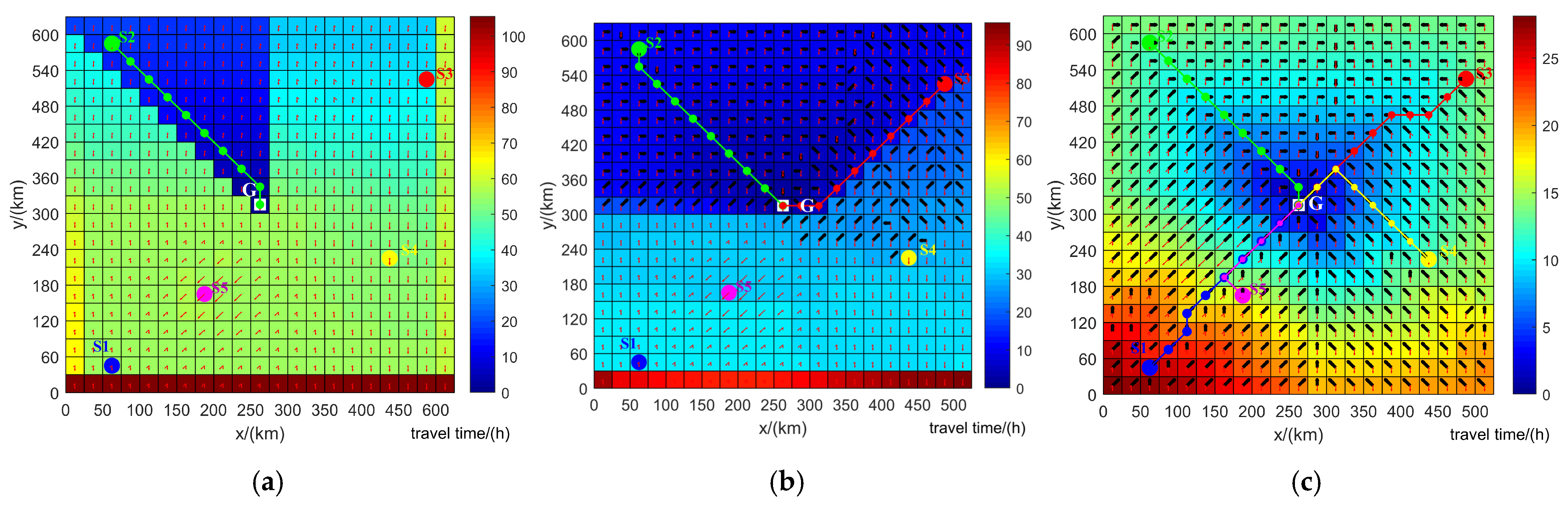
Within the flight airspace, multiple meteorological stations are present. Weight values are determined based on the distances to each station, as demonstrated in Equation (5), enabling the derivation of the 2D wind field distribution at a specific altitude within the flight area. The accuracy of the wind field distribution improves with an increased number of meteorological stations, as illustrated in Figure 3, which shows a schematic of weight determination when six stations are present in the flight area. Figure 4 depicts the 2D wind field distribution obtained using this method. In the figure, the arrow length corresponds to the wind speed magnitude (shorter arrows indicate weaker winds), while the arrow direction represents the wind direction. At this altitude, the prevailing wind is generally northerly, with notable spatial variations in the wind field.

$$\left\{\begin{array}{l}{x}_k={\displaystyle \sum _{j=1}^N{\alpha }_j{x}_j}={\alpha }_1{x}_1+{\alpha }_2{x}_2+\dots +{\alpha }_N{x}_N\\ y_k={\displaystyle \sum _{j=1}^N{\alpha }_j{y}_j}={\alpha }_1{y}_1+{\alpha }_2{y}_2+\dots +{\alpha }_N{y}_N\\ {\displaystyle \frac{{\alpha }_i}{{\alpha }_j}}=({\displaystyle \frac{d_j}{d_i}})i,j\le N\\ d_i=\sqrt{{(x_k-x_i)}^2+{(y_k-y_i)}^2}\\ {\displaystyle \sum _{j=1}^N{\alpha }_j}={\alpha }_1+{\alpha }_2\dots +{\alpha }_N=1\end{array}\right.,$$

(5)

where ${\alpha }_j$ represents the weight, $\left(x_k,y_k\right)$ denotes the coordinates of the goal location, and $d_i$ indicates the distance between the goal location and the known point.

3. 3D spatial distribution of wind fields

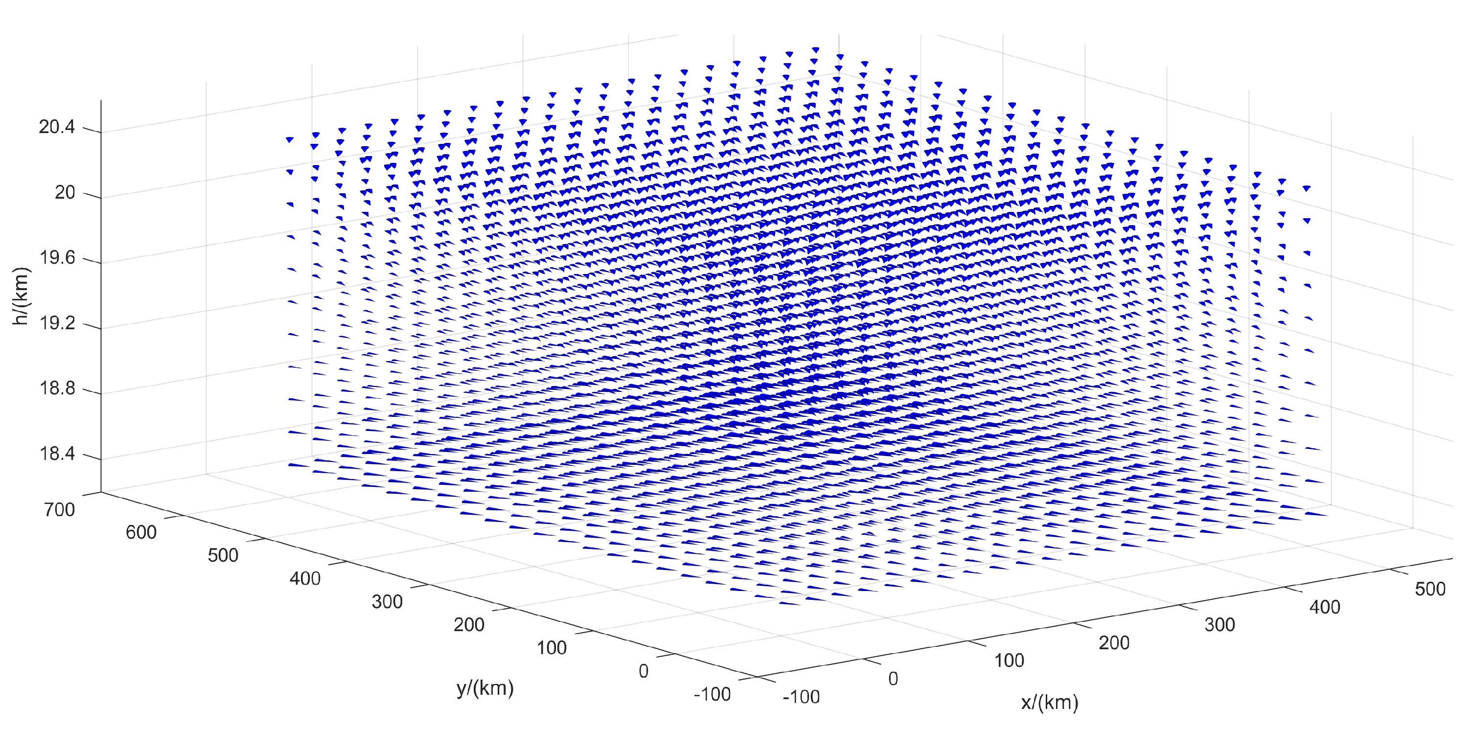
Vertical interpolation precision can be adjusted to obtain 3D wind field distributions with different numbers of wind layers. Figure 5 illustrates the distribution with 11 layers.

3.2.2. Establishing the Uncertain Wind Fields

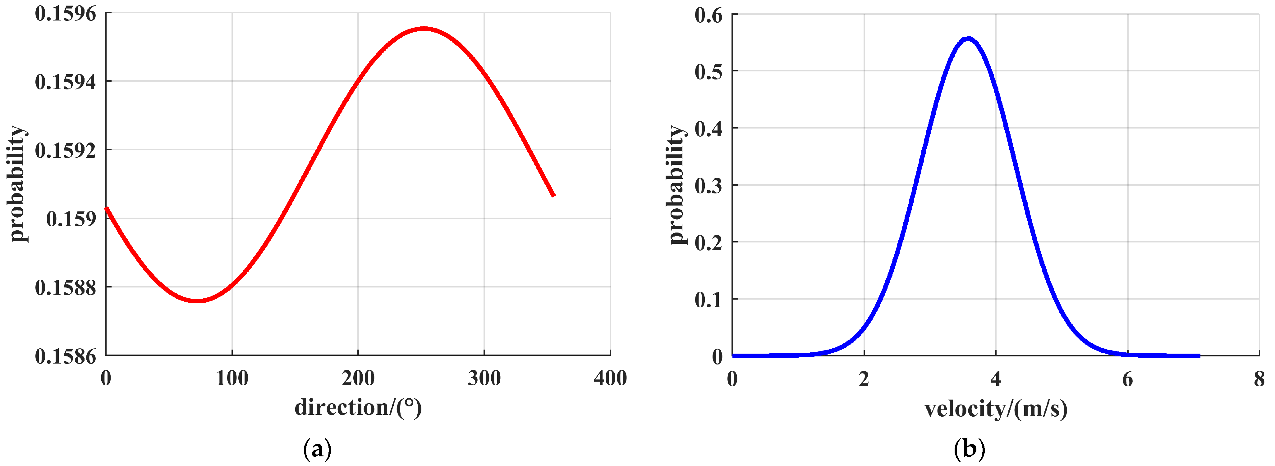
The wind field information $w({\mathit{r}}_i)$ includes wind direction and magnitude, respectively denoted by ${\theta }_i$ and $w_i$. These two variables exhibit mutually independent probability distributions. The wind direction probability follows a Von Mises distribution, with its probability density function given by Equation (6), while the wind speed probability adheres to a Gaussian distribution, as described by Equation (7).

$$f_{VM}({\theta }_i\left|\overline{{\theta }_i}\right.,\kappa )={\displaystyle \frac{\exp (\kappa \cos ({\theta }_i-\overline{{\theta }_i}))}{2\pi I_0(\kappa )}},$$

(6)

where $\overline{{\theta }_i}=\angle w({\mathit{r}}_i)$ denotes the actual wind direction, defined within the range $[0^{\circ },{360}^{\circ }]$. The parameter $\kappa (\kappa >0)$ represents the concentration parameter of the wind direction distribution, such that $\kappa \to 0$ indicates a more dispersed distribution, while $\kappa \to \infty$ corresponds to a more concentrated distribution. $I_0(\kappa )$ denotes the modified Bessel function of order 0.

$$f_{GS}(w_i\left|\overline{w_i}\right.,{\sigma }_i)={\displaystyle \frac{1}{{\sigma }_i\sqrt{2\pi }}}\exp (-{\displaystyle \frac{{\left(w_i-\overline{w_i}\right)}^2}{2{\sigma }_i^2}}),$$

(7)

where $\overline{w_i}=‖w({\mathit{r}}_i)‖$ denotes the mean wind, and the standard deviation is proportional to the magnitude ${\sigma }_i=\rho \overline{w_i}$ ($\rho$ is chosen by the user).

According to the predicted wind, at position $\mathit{r}={[\mathrm{0\; 0\; 19.4}]}^{\mathrm{T}}$, the direction is $\overline{{\theta }_i}={251.916}^{\circ }$, the magnitude is $\overline{w_i}=3.5756$, i.e., $\kappa =1/400$, $\rho =0.2$. The distribution of $\overline{{\theta }_i}$ and $\overline{w_i}$ are shown in Figure 6.

4. Approach

4.1. Research Object

The research object of this paper is an aerostat with weak horizontal propulsion and robust altitude regulation capabilities, which comprises eight subsystems: envelope structure, flight control, telemetry and control, altitude regulation, energy system, propulsion, environmental measurement, and recovery systems. The aerostat utilizes a photovoltaic–lithium battery hybrid energy system to provide sustained power for prolonged wind resistance and flight control operations. Critical components such as payloads, lithium batteries, flight controllers, and telemetry systems are housed within the pod, enabling recovery via parachute deployment or helium release through valves.

The horizontal propulsion capability is provided by the propulsion subsystem, which consists of four thrust units. Each unit delivers a maximum wind resistance capability of 5 m/s. The altitude regulation subsystem enables vertical maneuvering: air is pumped into ballast airbags via fans to increase the weight and descend, while releasing air through the valves reduces the weight to ascend. This subsystem allows for altitude adjustments within a range of ±1000 m around the stationary altitude.

4.2. Problem Setup

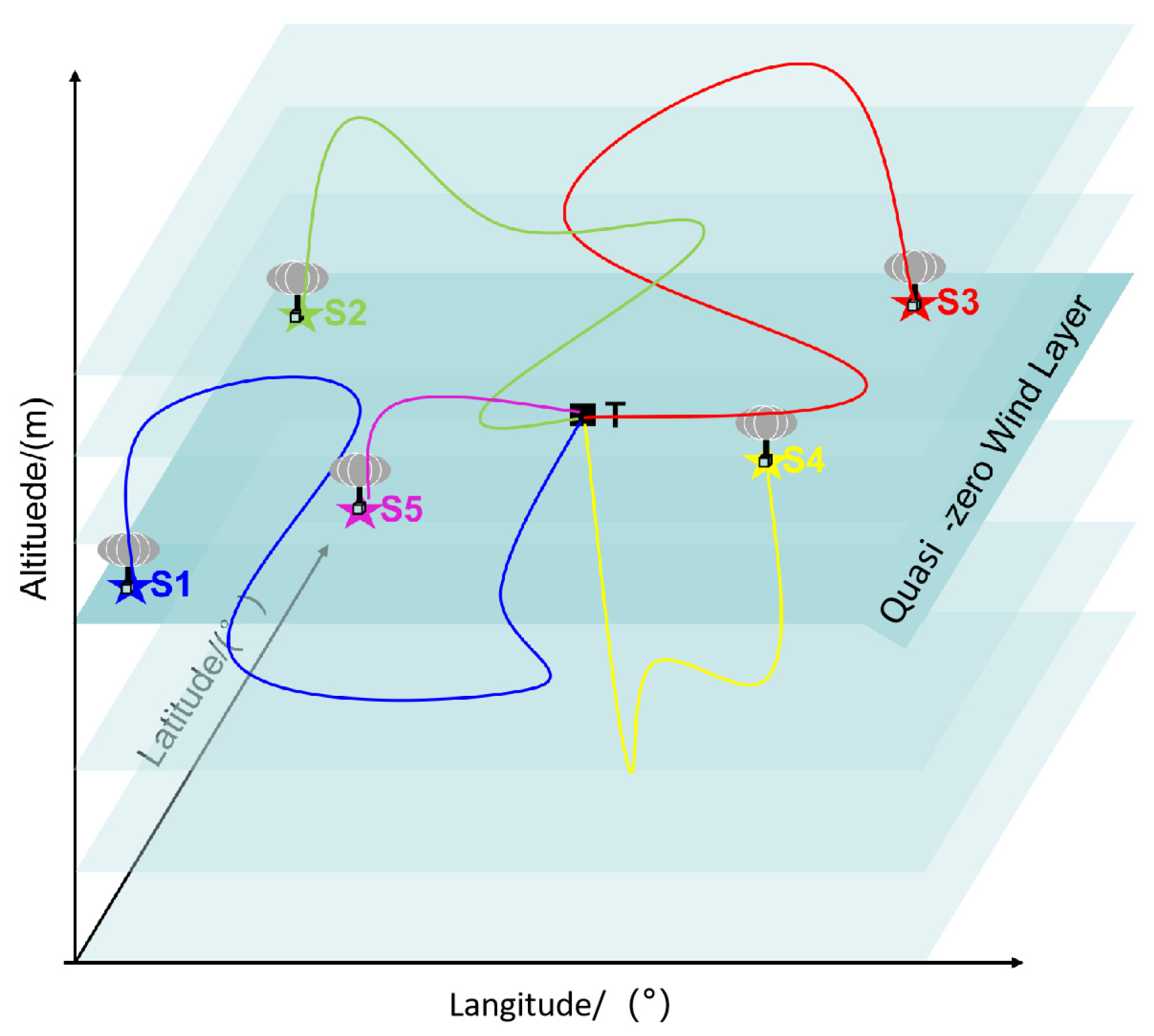
The aerostat is significantly influenced by wind fields, which exhibit marked variations with altitude and geographical location. Within the near-space, a quasi-zero-wind layer (typically below 5 m/s) often exists, flanked by opposing zonal winds at its upper and lower boundaries: a westerly belt beneath and an easterly belt above. In optimal path planning, the aerostat leverages these near-space wind characteristics to rationally select flight altitude and horizontal velocity, thereby enhancing flight efficiency, as illustrated in Figure 7.

The aerostat’s positional information is denoted by $\mathit{r}\triangleq {[x y z]}^{\mathrm{T}}$, where $x$ represents the east–west distance from the origin coordinate, $y$ denotes the north–south distance, and $z$ indicates altitude. Wind field data are represented by $w(\mathit{r})={[w(\mathit{r})\theta (\mathit{r}) w_z(\mathit{r})]}^{\mathrm{T}}$, with $w(\mathit{r})$ being the horizontal wind speed, $\theta (\mathit{r})$ being the horizontal wind direction (measured clockwise from the north), and $w_z(\mathit{r})$ being the vertical wind velocity. The aerostat’s velocity, relative to the air mass, is expressed as $u(\mathit{r})\triangleq {[u_x(\mathit{r}) u_y(\mathit{r})u_z(\mathit{r})]}^{\mathrm{T}}$, where $u_x(\mathit{r})$ and $u_y(\mathit{r})$ are the east–west and north–south thrust components provided by its propulsion subsystem, and $u_z(\mathit{r})$ is the altitude control velocity driven by its ballast system. The aerostat’s ground-relative velocity under wind influence is denoted by $\mathit{v}(\mathit{r})=\mathit{w}(\mathit{r})+\mathit{u}(s)$.

To concentrate on the core problem of optimal path planning for the aerostat, the following assumptions are made for the system:

(1) The aerostat is treated as a controllable point mass.

(2) When drifting horizontally without propulsion, its velocity aligns with the wind speed, and aerodynamic forces in the horizontal direction are neglected.

(3) Four independent propulsion units (motors and propellers) are mounted around the gondola to provide horizontal thrust. Each unit can generate a maximum counter-wind force, $u_{hor,\max }$, and the aerostat is constrained to operate two units simultaneously at most.

(4) The vertical wind speed in the near-space wind field is 0, and the wind field can be represented as $\mathit{w}(\mathit{r})\triangleq {[w(\mathit{r}) \theta (\mathit{r})]}^{\mathrm{T}}$.

(5) The altitude of the aerostat is controlled within the standing altitude ± 1000 m, denoted $v_{\mathit{r}ise}$ and $v_{sink}$.

The point-mass assumption (Assumption 1) is a standard simplification in trajectory planning when the focus is on center-of-mass motion. This is justified for the studied aerostat, due to its relatively low speed and control inputs primarily governing translational movement. For large-scale aerostats, the model can be extended to a 6-DOF formulation if needed.

The assumption of negligible vertical wind (Assumption 4) is based on characteristic meteorological conditions in the stratosphere [1,21]. Vertical winds are typically orders of magnitude smaller than horizontal winds, allowing for decoupling of horizontal planning from vertical dynamics. In scenarios with non-negligible vertical winds, the wind vector can be extended without altering the fundamental MDP framework.

Under these assumptions, the optimal path planning problem for the aerostat can be formulated as follows. The aerostat is modeled as an intelligent agent that is capable of sensing environmental states and making action decisions. The problem requires designing appropriate state spaces $S$, the set of actions $A$, and immediate reward $R$. Through iterative learning, the aerostat learns an optimal state-value function, enabling it to select optimal actions that minimize path-planning time. The objective is to achieve the shortest-time optimal trajectory and regional reachability analysis under complex constraints, including a predefined goal point, maximum counter-wind capacity, altitude control limits, and uncertain wind fields.

4.3. The Key Parameters of the MDP

4.3.1. Spatial Discretization and Transition

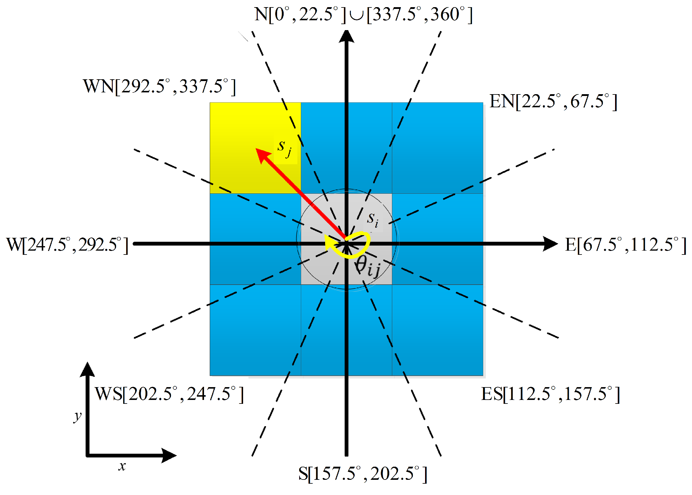
The spatial states are discretized using a grid-based method, where each grid cell represents the state information of the aerostat. The grid dimensions (denoted by $\Delta x$, $\Delta y$, $\Delta z$) correspond to the discretization resolutions in the east–west, north–south, and vertical directions, respectively. Spatial states encompass both the horizontal and vertical components. Initially, horizontal spatial discretization is performed, as illustrated in Figure 8. The gray grid signifies the aerostat’s current state, encoding its positional coordinates. Under the combined influence of wind fields and its inherent weak horizontal propulsion, the aerostat can transition horizontally to any of the eight adjacent states.

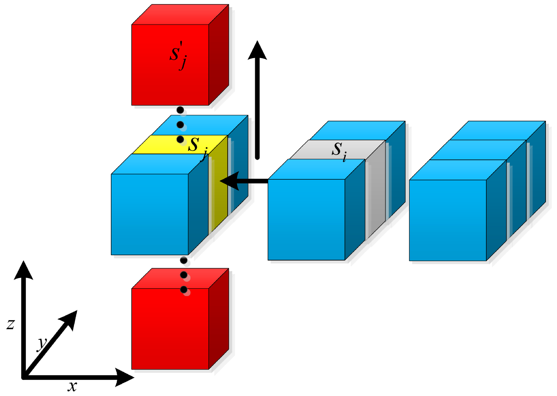
The aerostat adjusts its climbing/descending velocity by inflating or deflating auxiliary gas bags through fans and valves. During horizontal grid transitions, the vertical spatial states that are attainable by the aerostat are constrained by its maximum climbing/descending velocity, as illustrated in Figure 9. The limited vertical spatial states are discretized into an odd number $M$ of discrete states to represent height adjustments under different climbing/descending rates, thereby enabling discretization of the aerostat’s hovering altitude. A larger $M$ enhances altitude control precision but increases the number of grids generated and prolongs planning time. In practical path planning, it is essential to rationally determine the grid dimensions to balance the discretization accuracy and computational efficiency.

The aerostat is in its current state $s_i$, which allows for horizontal transitions to any of the eight adjacent grids $s_j$ with a transition time $\delta t$. For every state $s_i$, the local wind $\mathit{w}({\mathit{r}}_i)$ is selected at each visit from a probability distribution (the uncertain wind model is discussed above). After selecting the desired horizontal actuation, the aerostat velocity from $s_i$ can be written as follows:

$${\mathit{v}}_i=\mathit{w}({\mathit{r}}_i)+\left[u_x(s_i)u_y(s_i)\right],$$

(8)

where $u_x(s_i)$, $u_y(s_i)$ are the selected horizontal actuation components at state $s_i$ in the eastward and northward directions. The wind $\mathit{w}({\mathit{r}}_i)$ is constant in the interval until the next cell is reached. The time taken to travel from $s_i$ to $s_j$ is given by the following:

$$\delta t_i={\displaystyle \frac{dist({\mathit{r}}_i,{\mathit{r}}_j)}{{\mathit{v}}_i}},$$

(9)

where $dist(\cdot ,\cdot )$ is a function that returns the Cartesian distance between two states.

During the transfer period, the aerostat adjusts its vertical position to reach state ${s^{\prime }}_j$ within the vertical direction. The aerostat must satisfy specific constraints when in state ${s^{\prime }}_j$.

$$\left\{\begin{array}{l}x({s^{\prime }}_j)=x(s_j)\\ y({s^{\prime }}_j)=y(s_j)\\ z({s^{\prime }}_j)=u_z(s_i)·\delta t_i\\ z_0-1000\le z({s^{\prime }}_j)\le z_0-1000\end{array}\right.,$$

(10)

where $u_z(s_i)$ is the rise and sink rate at state.

The environmental state is characterized by wind field information, represented by wind direction and wind speed. The wind direction is discretized at 45° intervals, yielding eight discrete directions:

North (N): $[0^{\circ },{22.5}^{\circ }]\cup [{337.5}^{\circ },{360}^{\circ }]$

Northeast (EN): $[{22.5}^{\circ },{67.5}^{\circ }]$

East (E): $[{67.5}^{\circ },{112.5}^{\circ }]$

Southeast (ES): $[{112.5}^{\circ },{157.5}^{\circ }]$

South (S): $[{157.5}^{\circ },{202.5}^{\circ }]$

Southwest (WS): $[{202.5}^{\circ },{247.5}^{\circ }]$

West (W): $[{247.5}^{\circ },{292.5}^{\circ }]$

Northwest (WN): $[{292.5}^{\circ },{337.5}^{\circ }]$

During unpowered gliding, the transfer direction and drift speed of the aerostat are determined by the wind field information $w({\mathit{r}}_i)$. The wind field parameters remain constant during the transition from the current state $s_i$ to the next state ${s^{\prime }}_j$ and are updated $w({{\mathit{r}}^{\prime }}_j)$ upon reaching the destination state.

4.3.2. The Set of Actions

In the 3D path planning for aerostat, the set of actions includes horizontal actions and vertical actions. The horizontal actions are chosen from the following:

$$A_h=\left\{\mathbf{0},{\mathit{u}}_{h\max }{\widehat{\mathit{u}}}_1,{\mathit{u}}_{h\max }{\widehat{\mathit{u}}}_2,\dots ,u_{h\max }{\widehat{u}}_M\right\},$$

(11)

where $u_{h\max }$ is the maximum achievable horizontal actuation and ${\widehat{\mathit{u}}}_m$ is the unit vector pointing in each of the $M$ directions allowed. $M$ and ${\widehat{\mathit{u}}}_m$ are chosen by the users as part of the problem setup. We typically allow actuation in the direction of each horizontally adjacent cell and thus, $M=8$.

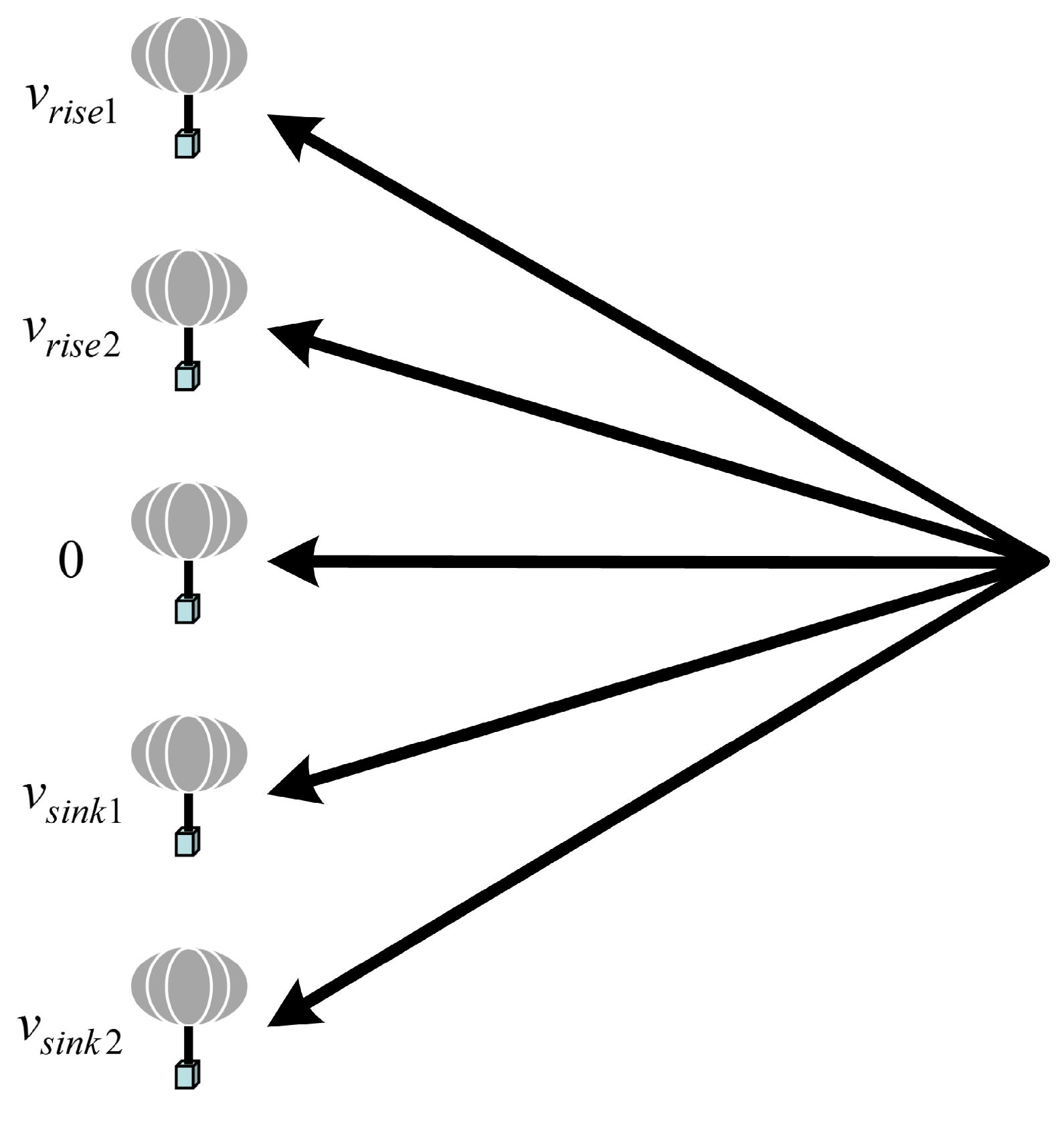
Vertical actions are discretized into five categories based on vertical space state discretization: level flight, climb/descent, and rapid climb/descent, as shown in Figure 10. The vertical actions are chosen from the following:

$$A_v=\left\{v_{rise1},v_{rise2},0,v_{sink1},v_{sink2}\right\},$$

(12)

where $v_{rise1}$ is the maximum rise rate, $v_{rise2}$ is the normal rise rate, $0$ is the horizontal flight, $v_{sink1}$ is the normal sink rate, and $v_{sink2}$ is the maximum sink rate.

4.3.3. Transition Probabilities

The transition probability function, denoted by $P_{a_{hor},a_{ver}}(s_i,{s^{\prime }}_j)$, represents the probability that the aerostat transitions from state $s_i$ to state ${s^{\prime }}_j$ after executing horizontal action $a_{hor}$ and vertical action $a_{ver}$. For horizontal transitions, the aerostat moves under the combined effects of uncertain wind fields and limited propulsion capability, leading to a probabilistic distribution of state $s_j$ from the current state $s_i$. In contrast, for vertical transitions, vertical winds are neglected; thus, the vertical movement from state $s_j$ to state ${s^{\prime }}_j$ is deterministic. However, the overall transition probability $P_{a_{hor},a_{ver}}(s_i,{s^{\prime }}_j)$ is governed by the uncertainty in wind fields, as horizontal dynamics dominate the probabilistic behavior:

$$P_{a_{hor},a_{ver}}(s_i,{s^{\prime }}_j)=P_{a_{hor}}(s_i,s_j)={\displaystyle \underset{{\theta }_{ij}}{\overset{{\theta }_{ij+4/\pi }}{\int }}{f}_{VM}(\theta \left|\overline{{\theta }_i}\right.,\kappa )}d\theta ,$$

(13)

where ${\theta }_{ij}$ represents the small boundary angle dividing the space into eight regions when transitioning from state $s_i$ to adjacent state $s_j$, as shown in Figure 10.

When the aerostat has wind resistance capability, the actual velocity during horizontal transitions is vactual ${\mathit{v}}_{i,a}=\mathit{w}({\mathit{r}}_i)+{\left[u_x(s_i)u_y(s_i)\right]}^{\mathrm{T}}$. The transition probabilities $P$ after executing each horizontal action are calculated using the Monte Carlo method, with the following steps:

Step 1: Wind field analysis. Using predicted wind field data, obtain the mean wind direction $\overline{{\theta }_i}$ and mean wind speed $\overline{w_i}$ for the current state $s_i$. Wind direction and wind speed probability distributions are then derived using the Von Mises distribution $f_{VM}(\theta \left|0\right.,\kappa )$ and Gaussian distribution $f_{GS}(w_i\left|0\right.,{\sigma }_i)$, respectively.

Step 2: Sample selection. Select sample points from the wind direction distribution ${\Theta }_i={\left\{{\theta }_i^n\right\}}_{n=1}^N$ and wind speed distribution $W_i={\left\{w_i^n\right\}}_{n=1}^N$.

Step 3: Velocity calculation. Based on the sampled wind direction, wind speed, and the horizontal action parameters, compute the aerostat’s actual velocity $V_{i,a_{hor}}={\left\{v_{i,a_{hor}}^n\right\}}_{n=1}^N$

$$V_{i,a_{hor}}=W_i{\left[\cos {\Theta }_i \sin {\Theta }_i\right]}^{\mathrm{T}}+{\left[u_x(s_i)u_y(s_i)\right]}^{\mathrm{T}},$$

(14)

Step 4: Transition probability estimation. Using the set of actual velocities $V_{i,a_{hor}}={\left\{v_{i,a_{hor}}^n\right\}}_{n=1}^N$, compute the transition probabilities $P_{a_{hor}}(s_i,s_j)$ for transitioning to the adjacent state $s_j$ from the current state $s_i$ after executing the horizontal action. $P_{a_{hor}}(s_i,s_j)$ is estimated by counting the samples whose resultant direction falls into the angular sector corresponding to $s_j$:

$$P_{a_{hor},a_{ver}}(s_i,{s^{\prime }}_j)=P_{a_{hor}}(s_i,s_j)={\displaystyle \frac{1}{N}}\left|V_{ij,a_{hor}}\right|,$$

(15)

where $\left| · \right|$ represents cardinality and $V_{ij,a_{hor}}=\left\{v_{i,a_{hor}}^n\left|\angle v_{i,a_{hor}}^n\in \left[{\theta }_{ij},{\theta }_{ij}+{\displaystyle \frac{\pi }{4}}\right]\right.\right\}$ is the angular sector for the adjacent cell.

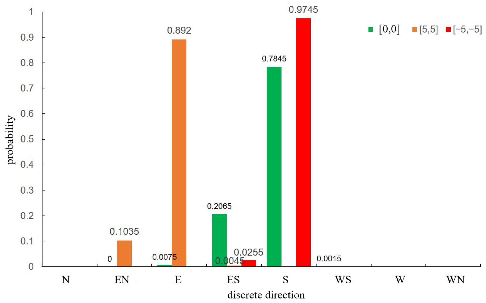
Based on the established uncertain wind field model, the probability distributions of wind direction $\overline{{\theta }_i}={251.916}^{\circ }$ and wind speed $\overline{w_i}=3.5756$ at position $\mathit{r}={[37° 86° 19000 \mathrm{m}]}^{\mathrm{T}}$ can be derived. The state transition probabilities of the aerostat under different horizontal actions (e.g., no propulsion, ${[5 5 0]}^{\mathrm{T}}$ and ${[-5 -5 0]}^{\mathrm{T}}$) are then calculated, as shown in Figure 11.

4.3.4. Immediate Reward

The immediate reward function $R_{a_{hor},a_{ver}}(s_i,{s^{\prime }}_j)$ represents the reward obtained by the aerostat when transitioning from state $s_i$ to state ${s^{\prime }}_j$ after executing horizontal action $a_{hor}$ and vertical action $a_{ver}$. This immediate reward consists of horizontal and vertical components: the horizontal reward is related to the transition time $\widehat{\delta t_{i,a_{hor}}}$, while the vertical reward depends on the wind field information $\mathit{w}({\mathit{r}}_i)$ of the selected wind layer. The specific steps are as follows:

Step 1: Compute the horizontal immediate reward $R_{a_{hor}}(s_i,s_j)$. Due to the probabilistic distribution of the aerostat’s actual speed caused by the uncertain wind field, the expected transition time is calculated using the mean velocity. The horizontal immediate reward is determined based on this expected transition time, which can be expressed as follows:

$$R_{a_{hor}}(s_i,s_j)=\left\{\begin{array}{ll}0,& \hfill \mathrm{reaching} \mathrm{goal} \mathrm{location}\\ -\widehat{\delta t_{i,a_{hor}}},& \hfill \mathrm{lose} \mathrm{to} \mathrm{goal} \mathrm{location}\\ -2\widehat{\delta t_{i,a_{hor}}},& \hfill \mathrm{away} \mathrm{from} \mathrm{goal} \mathrm{location}\\ -200,& \hfill \mathrm{out} \mathrm{of} \mathrm{boundary}\end{array}\right.,$$

(16)

where $\widehat{\delta t_{i,a_{hor}}}$ is the expected transition time from $s_i$ to $s_j$ under action $a_{hor}$, which can be calculated:

$$\left\{\begin{array}{l}〈v_{i,a_{hor}}〉={\displaystyle \frac{1}{N}}{\displaystyle \sum _{n=1}^N‖v_{i,a_{hor}}^n‖}\\ \delta t_{i,a_{hor}}={\displaystyle \frac{dist({\mathit{r}}_i,{\mathit{r}}_j)}{〈v_{i,a_{hor}}〉}}\\ \widehat{\delta t_{i,a_{hor}}}={\displaystyle \sum _{j\in S_i}{P}_{a_{hor}}(s_i,s_j)·}\delta t_{i,a_{hor}}\end{array}\right.,$$

(17)

Step 2: Determine the optimal wind layer. In the 3D wind field, wind characteristics vary significantly across different altitudes. After executing a vertical action $a_{ver}$, the aerostat reaches a specific wind layer. To identify the optimal wind layer, we rank the vertical actions based on the alignment of the wind at the resulting altitude with the direction to the goal:

$$x_{goal}-{x^{\prime }}_j\left\{\begin{array}{l}>0,w_x({{\mathit{r}}^{\prime }}_j)=max(w_x({{\mathit{r}}^{\prime }}_{jn}))\\ =0,w_x({{\mathit{r}}^{\prime }}_j)=min(|w_x({{\mathit{r}}^{\prime }}_{jn})|)\\ <0,w_x({{\mathit{r}}^{\prime }}_j)=min(w_x({{\mathit{r}}^{\prime }}_{jn}))\end{array}\right.,$$

(18)

$$y_{goal}-{y^{\prime }}_j\left\{\begin{array}{l}>0,w_y({{\mathit{r}}^{\prime }}_j)=max(w_y({{\mathit{r}}^{\prime }}_{jn}))\\ =0,w_y({{\mathit{r}}^{\prime }}_j)=min(|w_y({{\mathit{r}}^{\prime }}_{jn})|)\\ <0,w_y({{\mathit{r}}^{\prime }}_j)=min(w_y({{\mathit{r}}^{\prime }}_{jn}))\end{array}\right.,$$

(19)

where $n=1,2,\dots ,5$, which is the number of discretized vertical actions. $w_x({{\mathit{r}}^{\prime }}_{jn})$ and $w_y({{\mathit{r}}^{\prime }}_{jn})$ are east–west and north–south wind velocity components at the altitude reached after taking vertical action $a_{ver}$. $w_x({{\mathit{r}}^{\prime }}_j)$ and $w_y({{\mathit{r}}^{\prime }}_j)$ are the optimal east–west and north–south wind velocity.

Step 3: Calculate the vertical immediate reward. The vertical immediate reward is computed according to the ranking rules defined in Equations (18) and (19). This reward satisfies the criteria for both the east–west and north–south directions:

$$R_{a_{verx}}(s_i,{s^{\prime }}_j)/R_{a_{very}}(s_i,{s^{\prime }}_j)=\left\{\begin{array}{ll}0,& \hfill \mathrm{position} \mathrm{number} 1\\ -5,& \hfill \mathrm{position} \mathrm{number} 2\\ -10,& \hfill \mathrm{position} \mathrm{number} 3\\ -15,& \hfill \mathrm{position} \mathrm{number} 4\\ -20,& \hfill \mathrm{position} \mathrm{number} 5\end{array}\right.,$$

(20)

where a lower rank number (closer to one) indicates a more favorable wind layer

Step 4: Compute the vertical immediate reward weights ${\zeta }_x,{\zeta }_y$. Each wind layer has distinct east–west and north–south wind components. The weights for the vertical immediate reward in the east–west and north–south directions are determined based on the relative distance between the current position and the goal point:

$$\left\{\begin{array}{l}\Delta x=\left|x({\mathrm{s}}_{goal})-x(s_j)\right|\\ \Delta y=\left|y({\mathrm{s}}_{goal})-y(s_j)\right|\\ {\zeta }_x={\displaystyle \frac{\Delta x}{\Delta x+\Delta y}}\\ {\zeta }_y={\displaystyle \frac{\Delta y}{\Delta x+\Delta y}}\end{array}\right.,$$

(21)

where $\Delta x$ and $\Delta y$ denote the relative distances in the east–west and north–south directions between the current position and the target point, respectively.

Step 5: Calculate the immediate reward $R(s_i,{s^{\prime }}_j)$.

$$R(s_i,{s^{\prime }}_j)=R_{a_{hor}}(s_i,s_j)+{\zeta }_x{R}_{a_{verx}}(s_j,{s^{\prime }}_j)+{\zeta }_y{R}_{a_{very}}(s_j,{s^{\prime }}_j),$$

(22)

where $\zeta$ is a scaling factor to balance the two reward components.

4.3.5. Discount Factor

The global path planning problem is inherently a multi-step decision problem, where the optimality of the planning performance depends on long-term action sequences. The discount factor $\gamma$ quantifies the influence of future rewards on the cumulative reward. A larger discount factor emphasizes the impact of subsequent action selections on the state-value function, potentially altering the optimal path planning by prioritizing long-term rewards over immediate gains. In this work, we set $\gamma =0.95$.

4.4. The Flow of Optimal Path Planning

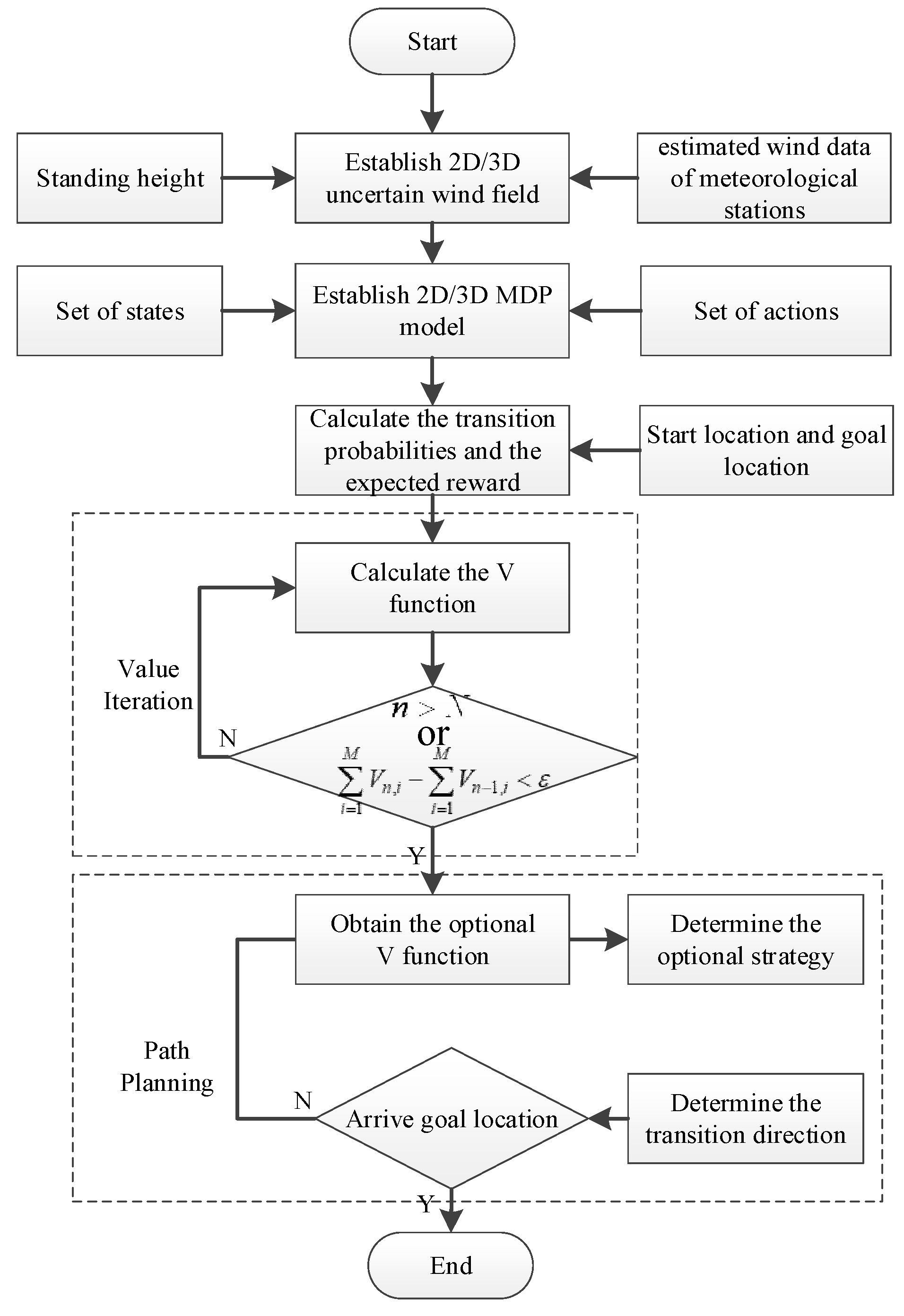
The optimal path planning algorithm for the high-altitude low-speed aerostat, which is based on MDP, primarily utilizes value iteration methods to compute the optimal state-value function. The policy corresponding to this function represents the optimal action sequence. The aerostat prioritizes transitions to the next states that minimize time consumption during state transitions by selecting actions in its current state. This approach enables the derivation of the shortest-time path for the aerostat. The algorithmic flow is depicted in Figure 12 and is outlined as follows:

Step 1: Input predicted meteorological data and station-keeping altitude. Establish an uncertain wind field model to characterize environmental dynamics.

Step 2: Define critical MDP model parameters, including the state space, action space, and transition probabilities.

Step 3: Input the coordinates of the start point and goal point. Calculate the immediate rewards and state transition probabilities.

Step 4: Calculate and iteratively update the state-value function using the value iteration algorithm.

Step 5: Terminate the iteration when either of the following conditions is met. The difference between two successive iterations of the state-value function falls below a convergence threshold $\epsilon$, or the maximum iteration count $n$ is reached. The resulting function is the optimal state-value function $V^{\ast }$.

Step 6: Derive the optimal policy ${\pi }^{\ast }$ for the current state, determine the transfer direction based on the policy, and execute the corresponding action. This action is ‘optimal,’ as it maximizes the expected cumulative reward from this state.

Step 7: Assess whether the transferred state has reached the goal point. If yes, terminate the process. If no, return to Step 6 to continue path planning.

5. Results

The study configures one goal point and five distinct start points, with five vertical actions (rapid descent, descent, level flight, ascent, rapid ascent) denoted as $[0,0,-0.1]$, $[0,0,-0.05]$, $[0,0,0]$, $[0,0,0.05]$, and $[0,0,0.1]$. The key parameters are set as follows: maximum wind resistance capability of a single propulsion system: 5 m/s; value iteration convergence threshold: $\epsilon =0.01$; maximum iteration count: $N=300$; and discount factor: $\gamma =0.95$. The proposed model and algorithm are applied to 2D and 3D optimal path planning for the high-altitude low-speed aerostat. By varying critical parameters, the effectiveness and engineering practicality of the path planning design parameters and procedures are validated.

5.1. 2D Optimal Path Planning

In practical missions, aerostats primarily operate in 2D horizontal planes at fixed altitudes (e.g., 19,400 m). The discretization precision is set to $nrow\times ncol=21\times 21$. Figure 13 illustrates the results under an uncertain wind field model for three scenarios:

No propulsion ($u_{\max }=0 \mathrm{m}/\mathrm{s}$);

Single propulsion system with 2 m/s wind resistance capability ($u_{\max }=2 \mathrm{m}/\mathrm{s}$);

Single propulsion system with 5 m/s wind resistance capability ($u_{\max }=5 \mathrm{m}/\mathrm{s}$).

The figure depicts the expected flight time, optimal action sequences, and optimal paths for all positions within the flight area to reach the goal point. The “optimal velocity direction” at each grid (indicated by black arrows) refers to the horizontal actuation prescribed by the optimal policy of the solved Markov decision process. It is the action that maximizes the cumulative reward (minimizes the expected time to the goal) from that state, given the uncertain wind field and system constraints. Thus, optimality is demonstrated by the policy extraction from the converged state-value function $V^{\ast }$ computed via value iteration. Key elements include the following:

White box: Goal point location.

Grid colors: Indicate expected flight time (bluer = shorter time; redder = longer time). Note the different color scales across subplots.

Red arrows: Wind direction and magnitude (arrow length corresponds to wind probability in that direction).

Black arrows: Optimal velocity direction for the aerostat at each grid position, derived from the optimal policy ${\pi }^{\ast }$.

Figure 13. 2D expected flight time distribution and optimal path planning: (a) $u_{\max }=0 \mathrm{m}/\mathrm{s}$; (b) $u_{\max }=2 \mathrm{m}/\mathrm{s}$; and (c) $u_{\max }=5 \mathrm{m}/\mathrm{s}$. (Black arrows represent the optimal resultant ground velocity direction derived from the converged optimal policy ${\pi }^{\ast }$).

Figure 13. 2D expected flight time distribution and optimal path planning: (a) $u_{\max }=0 \mathrm{m}/\mathrm{s}$; (b) $u_{\max }=2 \mathrm{m}/\mathrm{s}$; and (c) $u_{\max }=5 \mathrm{m}/\mathrm{s}$. (Black arrows represent the optimal resultant ground velocity direction derived from the converged optimal policy ${\pi }^{\ast }$).

5.1.1. Regional Reachability Analysis

By comparing the information in Figure 13, we can obtain:

Without propulsion (Figure 13a): The aerostat can only drift with wind. Only a few positions northwest of the goal point can reach the goal quickly.

With $u_{\max }=2 \mathrm{m}/\mathrm{s}$ (Figure 13b): The aerostat can reach the target within 20 h from nearly all northern positions relative to the target.

With $u_{\max }=5 \mathrm{m}/\mathrm{s}$ (Figure 13c): The aerostat achieves universal reachability (expected flight time within 20 h from nearly all positions in the flight area).

Regional reachability is defined as the ratio of reachable positions to total positions.

Table 2. Regional reachability under different horizontal actuation.

Max. Horizontal Actuation	Number of Reachable Cells	Regional Reachability
$u_{\max }=0 \mathrm{m}/\mathrm{s}$	56	12.7%
$u_{\max }=2 \mathrm{m}/\mathrm{s}$	251	56.9%
$u_{\max }=5 \mathrm{m}/\mathrm{s}$	441	100%

summarizes the regional reachability under different wind resistance capabilities, demonstrating that enhanced wind resistance significantly improves reachability in uncertain wind fields.

5.1.2. The Optimal Path and Strategy Planning

The aerostat’s optimal strategy (i.e., optimal action sequences) executed from different positions yields the optimal path, as shown in Figure 13. The aerostat’s wind resistance capability, start point locations, and other factors influence the planning of optimal strategies and paths.

Table 3. Comparison of the planned 2D optimal paths under different conditions.

Start Point	Max. Horizontal Actuation	Numbers of Optimal Path Notes	Flight Time (h)
Start Point 1	$u_{\max }=5 \mathrm{m}/\mathrm{s}$	9	24.9
Start Point 2	$u_{\max }=0 \mathrm{m}/\mathrm{s}$	9	21.33
	$u_{\max }=2 \mathrm{m}/\mathrm{s}$	9	15.79
	$u_{\max }=5 \mathrm{m}/\mathrm{s}$	9	16.08
Start Point 3	$u_{\max }=2 \mathrm{m}/\mathrm{s}$	9	17.84
	$u_{\max }=5 \mathrm{m}/\mathrm{s}$	9	16.45
Start Point 4	$u_{\max }=5 \mathrm{m}/\mathrm{s}$	7	11.62
Start Point 5	$u_{\max }=5 \mathrm{m}/\mathrm{s}$	5	20.91

summarizes the number of path nodes and flight time for optimal paths under different conditions. Taking Start Point 2 as an example, Figure 13 shows that optimal paths and strategies for the same start point differ under varying conditions (e.g., wind resistance capabilities). However, as shown in Table 3, increasing wind resistance capability drastically reduces the flight time to the goal point for the same start point.

5.2. 3D Optimal Path Planning

5.2.1. Regional Reachability Analysis

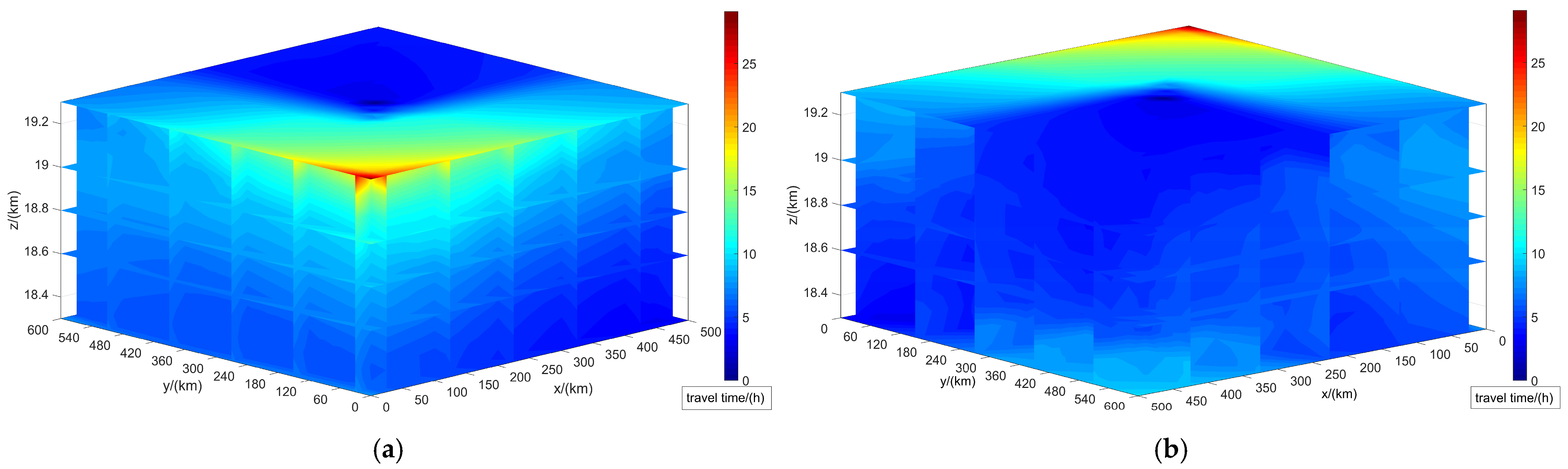
The aerostat ascends and stabilizes at its designed station-keeping altitude, then employs the aforementioned model and method to reach the goal position in the shortest possible time without specifying the final altitude. Figure 14 illustrates the distribution of the expected flight time to the goal point under a maximum wind resistance capability of 5 m/s, with different start points. The redder the color in the figure, the longer the expected flight time to the goal point at that location.

As shown in Figure 6 and Figure 14, the eastward wind component increases with an altitude above 19,400 m. Consequently, the aerostat must counteract adverse wind effects more significantly at altitudes exceeding 20,000 m, leading to a longer expected flight time. Notably, the aerostat achieves global reachability throughout the 3D area under these conditions.

5.2.2. The Optimal Path and Strategy Planning

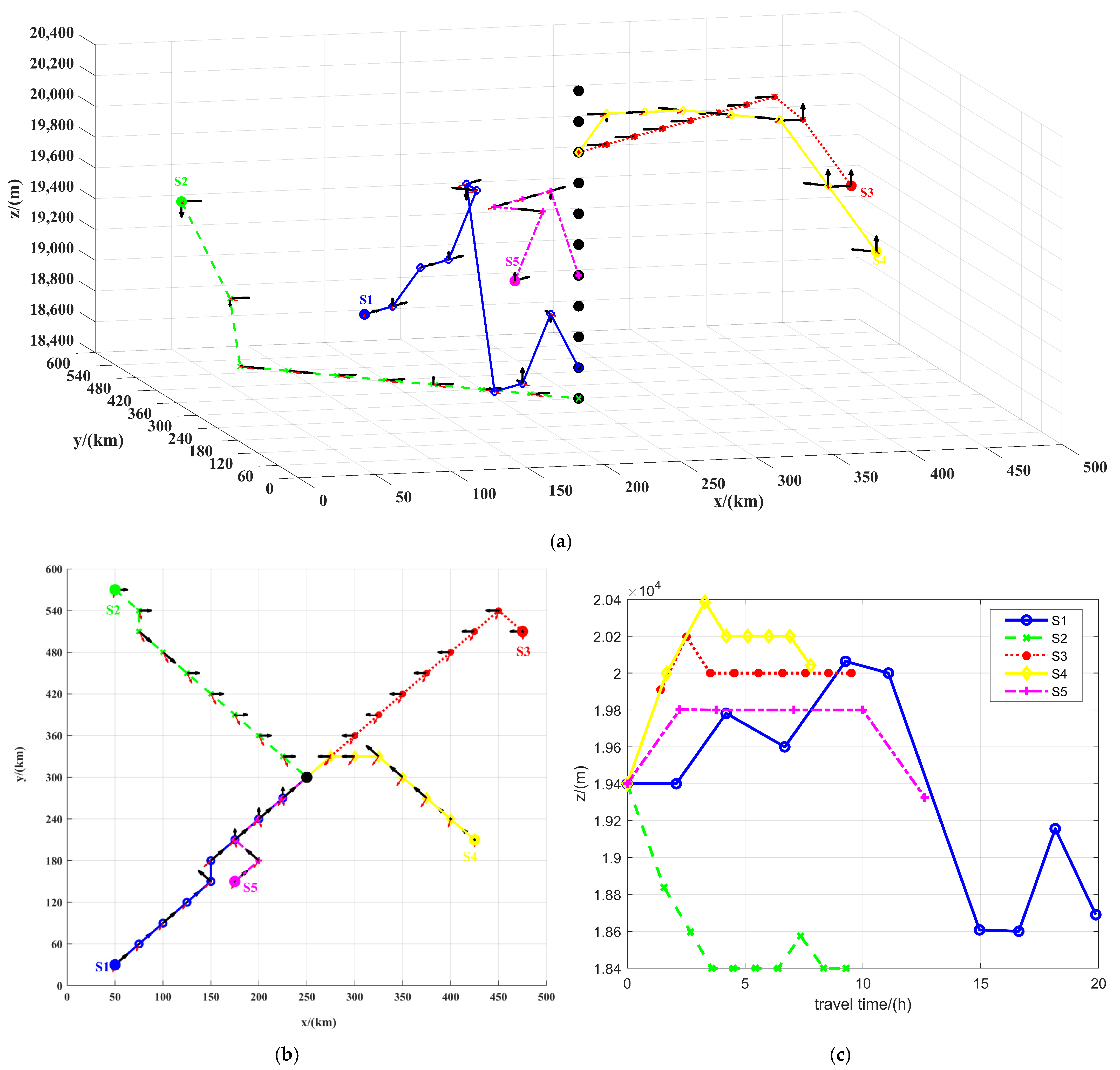
The 3D optimal path planning and strategy depend on factors such as wind field distribution, maximum wind resistance capability, altitude adjustment ability, and start point location. Figure 15 depicts the optimal paths and strategies, as well as the altitude variations over time for paths planned from the five start points.

Table 4. Comparison of the planned 3D optimal paths.

Start Point	Number of Altitude Controls	Numbers of Path Notes	Flight Time (h)
Start Point 1	7	9	19.88
Start Point 2	5	9	9.29
Start Point 3	2	9	9.51
Start Point 4	3	7	7.78
Start Point 5	2	5	12.62

compares 3D optimal paths under different conditions.

Black arrows indicate the aerostat’s executed actions at specific locations. Horizontal arrows denote selected horizontal movement directions. Vertical arrows indicate vertical altitude adjustments, with a length that is proportional to the adjustment speed. The absence of vertical arrows signifies a level flight (no altitude change).

Red arrows represent the wind field information at each location, with direction indicating wind direction and length proportional to wind speed.

From Figure 15 and Table 4, we can obtain the following.

• Start Points 1 and 2: Both are west of the goal, but Start Point 1 is north and Start Point 2 is south. To better exploit the 3D wind field, their optimal paths exhibit distinct altitude variations: From Start Point 1, the altitude increases, then decreases, and increases again. From Start Point 2, the altitude first decreases, then remains stable, then increases.
• Start Points 3 and 4: Their paths show similar altitude changes because both are east of the goal and require locating optimal eastward wind layers to minimize flight time.
• Start Points 1 and 5: Both are southwest of the goal but at different distances. Their strategies for locating favorable wind layers differ, leading to disparate altitude adjustments.
• Start Point 4 achieves the shortest flight time for the simulated conditions, making it the most favorable among the evaluated deployment options in this scenario. 3D paths from the same start point consistently outperform 2D paths in terms of flight time, demonstrating the aerostat’s capability to leverage vertical wind layers for rapid deployment.
• Start Point 2 is closest to the goal, yet its expected flight time is not the shortest, underscoring the dominant influence of wind fields on path efficiency. The aerostat’s altitude adjustment capability significantly enhances deployment efficiency by enabling adaptive navigation through vertical wind layers.

To determine the optimal launch point among the five candidates, the proposed MDP-based optimization framework was applied to each start point independently under identical environmental and constraint settings. The resulting flight times (presented in Table 4) were then compared systematically. Start Point 4 yielded the shortest planned flight time (7.78 h), thereby identifying it as the optimal choice for mission deployment under the given conditions. This conclusion is a direct output of the comparative optimization process, not a post hoc observation.

The aerostat’s wind resistance capability critically impacts the regional reachability and path planning. With altitude adjustment ability, the aerostat can further optimize flight time by exploiting 3D wind field variations, achieving rapid and reliable deployment to target locations.

5.3. Comparative Analysis and Performance Evaluation

5.3.1. Baseline Methods

Two distinct baseline planners were implemented to contextualize the performance of our proposed 3D-MDP method:

• Fixed-altitude MDP (2D-MDP): This method utilizes the same MDP core (state transition, reward) as our proposed framework but is constrained to operate at a single, fixed altitude (the initial flight level of 19,400 m). The vertical action set is disabled. This baseline serves to isolate and quantify the performance gain that is solely attributable to the strategic 3D altitude selection capability of our full method.
• Greedy Heuristic algorithm: At each decision step, this reactive planner selects the combination of allowable horizontal and vertical actions that immediately minimizes the Euclidean distance to the goal position, given the current local wind estimate and propulsion limits. It performs no long-term value iteration or planning. This baseline represents a myopic, locally optimal strategy and highlights the value of global, foresighted planning under uncertainty that is offered by the MDP framework.

5.3.2. Evaluation Metrics

Three key performance indicators (KPIs) were employed for a multi-faceted evaluation:

Average flight time (AFT) [hours]: The mean time taken to successfully reach the goal point across all successful Monte Carlo simulation runs. A lower value indicates higher efficiency.

Success rate (SR) [%]: The percentage of simulation runs (out of 100 Monte Carlo trials per start point) that reached the goal within a maximum allowed mission time (set to 30 h for this study). A higher value indicates greater reliability.

Temporal robustness (σ) [hours]: The standard deviation of the flight time across successful runs. A lower standard deviation signifies less variability and greater predictability in the planned path’s duration when facing the same wind uncertainty, which is critical for mission scheduling.

5.3.3. Comparative Results and Discussion

All three methods were evaluated under identical conditions: the same five start points (SP1-SP5), the identical probabilistic wind field model, and the same platform constraints (e.g., maximum thrust of 5 m/s).

Table 5. Performance comparison of the proposed 3D-MDP method against baseline planners.

Start Point	Method	Avg. Flight Time (h) ↓	Std. Dev. (h) ↓	Success Rate (%) ↑
Start Point 1	3D-MDP (Proposed)	19.88	2.1	92
	2D-MDP (Fixed-Altitude)	25.34	3.3	85
	Greedy Heuristic	28.91	5.8	70
Start Point 2	3D-MDP (Proposed)	9.29	1.2	98
	2D-MDP (Fixed-Altitude)	12.15	2.8	90
	Greedy Heuristic	15.40	4.5	75
Start Point 3	3D-MDP (Proposed)	9.51	1.5	97
	2D-MDP (Fixed-Altitude)	11.92	2.9	88
	Greedy Heuristic	17.84	5.2	72
Start Point 4	3D-MDP (Proposed)	7.78	0.9	99
	2D-MDP (Fixed-Altitude)	10.23	2.0	93
	Greedy Heuristic	13.57	3.8	80
Start Point 5	3D-MDP (Proposed)	12.62	1.8	95
	2D-MDP (Fixed-Altitude)	16.45	3.2	87
	Greedy Heuristic	20.91	4.7	78

Note: Arrows indicate the desirable direction for each metric (↓ lower is better, ↑ higher is better). Bold values denote the best performance for a given start point.

summarizes the aggregated results from 100 Monte Carlo trials per method per start point.

The results in Table 5 lead to several unambiguous conclusions regarding the clear effect of the proposed research:

• Superiority in deployment efficiency and reliability: The proposed 3D-MDP method consistently outperforms both baselines across all start points and all metrics. It achieves the shortest average flight times (AFT) and the highest success rates (SR). For instance, at SP1, 3D-MDP reduces the AFT by 21.5% compared to the 2D-MDP and by 31.2% compared to the Greedy algorithm, while simultaneously improving SR by 7 and 22 percentage points, respectively. This conclusively demonstrates that integrating strategic altitude control into a global MDP planner is highly effective for minimizing deployment time and ensuring mission success under uncertainty.
• Enhanced robustness and predictability: A key, clear finding is the superior temporal robustness of the 3D-MDP method, evidenced by its consistently lowest standard deviation (σ) in flight time. This indicates that our method not only plans faster paths but also plans more consistent and predictable ones. The lower variance means the actual flight time is less susceptible to the specific instantiations of wind uncertainty, providing mission planners with more reliable time estimates—a critical practical advantage.
• Disentangling the contributions of planning foresight and altitude control:

  (1)

  Global planning vs. myopic reaction: The substantial performance gap between 3D-MDP and the Greedy Heuristic (e.g., ~50% longer flight times and ~20% lower success rates for Greedy at SP3) provides direct evidence that a foresighted, global optimization strategy is fundamentally superior to a reactive, locally optimal one in a stochastic, wind-dominated environment.

  (2)

  Value of 3D altitude optimization: The consistent and significant advantage of 3D-MDP over the 2D-MDP baseline directly quantifies the value of active altitude selection. By dynamically choosing flight levels to exploit favorable wind layers (as visualized in Section 4.2), the 3D-MDP method achieves faster and more reliable paths even than what is possible with an optimal planner restricted to a fixed altitude.

6. Discussion

This article investigates aerostats equipped with limited horizontal propulsion and altitude adjustment capability, addressing uncertainties in wind data caused by factors such as the prediction accuracy of wind field models. An MDP-based optimal path planning method is proposed to address these challenges. The method formulates path planning as identifying the optimal path with the shortest flight time from the current position to the goal point under given environmental conditions and reward–punishment criteria. By designing critical parameters and algorithmic workflows—including the set of actions, immediate reward function, and state transition probability function—the method enables 2D/3D regional reachability analysis and global path planning from the starting point to the goal point under complex constraints such as uncertain wind fields, horizontal wind resistance capability, altitude adjustment capability and flight time.

The proposed methodology yields three critical insights:

• Effective handling of uncertain wind fields. The method effectively addresses the optimal path planning problem for high-altitude low-speed aerostats under uncertain wind fields, providing a more practically relevant environmental foundation for path planning.
• Quantitative assessment of wind resistance impact. It quantitatively evaluates the impact of factors such as wind resistance capability on regional reachability, offering guidance for selecting optimal starting points for aerostats.
• Comprehensive path and strategy generation. The method generates optimal paths and strategies for all positions within a given flight area, providing a theoretical basis for the practical deployment and actuation strategies of aerostats.

7. Conclusions

This paper addressed the optimal path planning problem for high-altitude low-speed aerostats under complex constraints. A novel MDP-based method was proposed, integrating a probabilistic wind uncertainty model with the aerostat’s physical constraints into a unified framework.

The core contributions are: (1) development of a probabilistic wind field model capturing forecast errors, (2) formulation of a constraint-aware MDP incorporating propulsion and altitude limits, and (3) implementation of a 3D altitude-aware planning algorithm enabling quantitative reachability analysis.

Simulation results demonstrated method effectiveness. In 2D planning, increased wind resistance improved reachability. In 3D planning, dynamic altitude selection reduced deployment time. The method successfully generated time-optimal paths from multiple start points.

Future work could focus on: integrating real-time wind forecast updates, optimizing energy consumption, validating with high-fidelity models or real data, and extending to a POMDP framework for imperfect state information.

References

1. Belmont, A.D.; Dartt, D.G.; Nastrom, G.D. Variations of stratospheric zonal winds, 20–65 km, 1961–1971. J. Appl. Meterology 2010, 14, 585–594. [Google Scholar] [CrossRef]
2. Hong, Y.J. Aircraft Technology of Near Space; National Defense Industry Press: Beijing, China, 2012. [Google Scholar]
3. Zhai, J.Q.; Yang, X.X.; Dend, X.L. Global path planning of stratospheric aerostat in uncertain wind field. Beijing Univ. Aeronaut. Astronaut. 2023, 49, 1116–1126. [Google Scholar] [CrossRef]
4. Lin, K.; Ma, Y.P.; Zheng, Z.W.; Wu, Z. Height control of stratospheric aerostat based on secondary airbag. Beijing Univ. Aeronaut. Astronaut. 2022, 48, 762–770. [Google Scholar]
5. Yang, Y.C.; Cao, H.S.; Zhao, R.; Zhu, R.C.; Song, L. Modeling and numerical simulation of constant-height flight by air-lifting gas mixing for aerostats. J. Natl. Univ. Def. Technol. 2023, 45, 196–204. [Google Scholar]
6. Deng, X.; Yang, X.; Zhu, B.; Ma, Z.; Hou, Z. Simulation research and key technologies analysis of intelligent stratospheric aerostat Loon. ACTA Aeronaut. Astronaut. Sin. 2023, 44, 127412. [Google Scholar]
7. Huang, D.J.; Jiang, C.F.; Han, K.L. 3D Path Planning Algorithm Based on Deep Reinforcement Learning. Comput. Eng. Appl. 2020, 56, 30–36. [Google Scholar]
8. Khatib, O. Real-time obstacle avoidance for manipulators and mobile robots. Int. J. Robot. Res. 1986, 5, 90–98. [Google Scholar] [CrossRef]
9. Wolf, M.T.; Blackmore, L.; Kuwata, Y. Probabilistic motion planning of balloons in strong, uncertain wind fields. In Proceedings of the 2010 IEEE International Conference on Robotics and Automation, Anchorage, AK, USA, 3–7 May 2010; IEEE: Piscataway, NJ, USA, 2010; pp. 1123–1129. [Google Scholar]
10. Zheng, B.J.; Guo, X.; Wang, Y.F.; Ou, J.J.; Lou, W.J. Deep-Reinforcement-Learning-Based Path Planning Method for Stratospheric Airships in Spatiotemporally Complex Environments. IEEE Trans. Aerosp. Electron. Syst. 2025, 61, 17843–17857. [Google Scholar] [CrossRef]
11. Lyu, Z.; Gao, Y.; Chen, J.; Du, H.; Xu, H.; Huang, K.; Kim, D.I. Empowering Intelligent Low-Altitude Economy With Large AI Model Deployment. IEEE Wirel. Commun. 2026. early access. [Google Scholar] [CrossRef]
12. Zhao, W.Y.; He, T.R.; Chen, R.; Wei, T.H.; Liu, C.L. State-wise Safe Reinforcement Learning: A Survey. In Proceedings of the 32nd International Joint Conference on Artificial Intelligence (IJCAI), Macao, China, 19–25 August 2023; pp. 6814–6822. [Google Scholar]
13. Yu, X.; Zhou, X.; Zhang, Y. Collision-free trajectory generation and tracking for UAVs using Markov decision process in a cluttered environment. J. Intell. Robot. Syst. 2019, 93, 17–32. [Google Scholar] [CrossRef]
14. Sun, Y.; Wang, L.; Wu, J. A general overview of path planning methods for autonomous underwater vehicle. Ship Sci. Technol. 2020, 4, 1–7. [Google Scholar]
15. Chen, L.; Duan, D.P.; Sun, D.S. Design of a multi-vectored thrust aerostat with a reconfigurable control system. Aerosp. Sci. Technol. 2016, 53, 95–102. [Google Scholar] [CrossRef]
16. Zhao, M.; Xiao, C.; Zhou, P.F.; Duan, D.P. Dynamics modeling and simulation of a saucer-shaped stratospheric aerostat with an under-slung nacelle. J. Cent. South Univ. 2017, 24, 1288–1298. [Google Scholar] [CrossRef]
17. Bordalba, R.; Ros, L.; Porta, J.M. Randomized Kinodynamic Planning for Constrained Systems. In Proceedings of the 2018 IEEE International Conference on Robotics and Automation (ICRA), Brisbane, QLD, Australia, 21–25 May 2018; IEEE: Piscataway, NJ, USA, 2018; pp. 7079–7086. [Google Scholar]
18. Goldberg, D.E. Genetic Algorithms in Search, Optimization and Machine Learning; Addison-Wesley: Boston, MA, USA, 1989. [Google Scholar]
19. Sutton, R.S.; Barto, A.G. Reinforcement Learning: An Introduction; MIT Press: Cambridge, MA, USA, 2018; pp. 10–87. [Google Scholar]
20. Ruan, X.; Ren, D.; Zhu, X. Mobile robot navigation based on deep reinforcement learning. In Proceedings of the 2019 Chinese Control and Decision Conference (CCDC); IEEE: Piscataway, NJ, USA, 2019; pp. 6174–6178. [Google Scholar]
21. Liu, K. Practical Markov Decision Making Process; University of Tsinghua Press: Beijing, China, 2012; pp. 9–12. [Google Scholar]
Figure 1. Model of MDP.
Drones 10 00128 g001
Figure 2. Profiles for the zonal wind with the altitude at six stations.
Drones 10 00128 g002
Figure 3. Diagram of determining weights in a 2D plane. (Star system: Target position; Red arrow: Straight-line distance between the weather station and target; Green circle: Weather station.).
Drones 10 00128 g003
Figure 4. 2D spatial distribution of wind fields at a specific altitude. (The arrow direction indicates the wind direction.).
Drones 10 00128 g004
Figure 5. 3D spatial distribution of wind fields (11 layers). (The direction of the blue arrows represents the wind direction, and the length of the arrows indicates the wind speed.).
Drones 10 00128 g005
Figure 6. Distribution of wind direction and velocity under uncertain model: (a) wind direction distribution and (b) wind velocity distribution.
Drones 10 00128 g006
Figure 7. Schematic of 3D path planning leveraging wind layers. (The pentagram represents different starting positions, the black square represents the target position, and different curves represent the paths from the starting points to the target point.).
Drones 10 00128 g007
Figure 8. Schematic of horizontal state discretization and possible transitions under wind and propulsion. (The gray grid represents the current position s i , the yellow grid represents the next position s j to be transferred, the blue grid represents other possible transfer positions, the red arrow indicates the transfer direction, and the yellow arrow represents the transfer angle θ i j ).
Drones 10 00128 g008
Figure 9. Schematic of horizontal and vertical state discretization and possible transitions under wind and propulsion. (The gray grid represents the current position s i , the yellow grid represents the next position s j for horizontal transfer, the red grid represents the next position s j for vertical transfer, and the blue grid represents other possible transfer positions).
Drones 10 00128 g009
Figure 10. Vertical state discretization and altitude transition constraints under maximum climb/sink rates. (The black arrows indicate the possible positions that the aerostat can reach from the current position with different vertical velocities.).
Drones 10 00128 g010
Figure 11. Transition probability distributions under different horizontal actuation levels.
Drones 10 00128 g011
Figure 12. Flowchart of the proposed MDP-based path planning method.
Drones 10 00128 g012
Figure 14. 3D expected flight time distribution under u max = 5   m / s : (a) view from the increasing altitude side and (b) view from the decreasing altitude side.
Drones 10 00128 g014
Figure 15. 3D optimal path planning results: (a) planned 3D optimal paths and strategies; (b) planform of the 3D optimal paths and strategies; and (c) altitude variations in the planned 3D optimal paths over time.
Drones 10 00128 g015