Adaptive Backstepping Sliding Mode Control for Direct Driven Hydraulics ^†

Abstract

Due to the advantages of high energy efficiency and environmental friendliness, the electro-hydraulic actuator (EHA) plays a vital role in fluid power control. One variant of EHA, double pump direct driven hydraulics (DDH), is proposed, which consists of double fixed-displacement pumps, a servo motor, an asymmetric cylinder and auxiliary components. This paper proposes an adaptive backstepping sliding mode control (ABSMC) strategy for DDH to eliminate the adverse effect produced by parametric uncertainty, nonlinear characteristics and the uncertain external disturbance. Based on theoretical analysis, the nonlinear system model is built and transformed. Furthermore, by defining the sliding manifold and selecting a proper Lyapunov function, the nesting problems (of the designed variable and adaptive law) caused by uncertain coefficients are solved. Moreover, the adaptive backstepping control and the sliding mode control are combined to boost system robustness. At the same time, the controller parameter adaptive law is derived from Lyapunov analysis to guarantee the stability of the system. Simulations of the DDH are performed with the proposed control strategy and proportional–integral–differential (PID), respectively. The results show that the proposed control strategy can achieve better position tracking and stronger robustness under parameter changing compared with PID.

1. Introduction

The hydraulic system is widely used in robots, automobiles, aerospace and defence industries due to its advantages, such as fast response, high force and power density, reliability and robustness [1]. The system can be divided into two categories: the valve-controlled system and the pump-controlled system. Owing to the high accuracy and low-cost, the valve-controlled system is adopted more. However, with the energy crisis and pollution issue, the pump-controlled system has attracted rising attention because of its higher energy efficiency. In terms of energy, the pump-controlled system eliminates significant throttling loss, which accounts for 44% of the energy loss of the valve-controlled system [2,3].

One division of pump-controlled system, the electro-hydraulic actuator (EHA), is usually referred to a compact and reliable self-contained unit composed of the electric motor, pump/motors, hydraulic cylinder and auxiliary components. EHA can be divided into three classifications: (1) fixed displacement pump and variable speed electric motor, (2) variable displacement pump and fixed speed electric motor and (3) variable displacement pump and variable speed electric motor. The third configuration can provide the highest energy efficiency, but it costs more and requires more complex control systems to achieve maximum efficiency [4,5]. Compared to the other two classifications, the first scheme has the slowest dynamic response, but it has the properties of low-cost, simplicity and high-efficiency [5,6,7,8]. Hence, it attracts increasing attention. However, there are strong nonlinearities and uncertainties in EHA, such as nonlinear friction, parameter uncertainty and unknown external disturbances. Therefore, the controller design of the EHA faces significant challenges [9].

Due to the uncertainty and disturbance in the whole system, the control performance cannot be guaranteed by applying the proportional–integral–derivative (PID) control method [10]. Hence, many studies related to the position control of the EHA are conducted. Among them, some control strategies have achieved high-performance in position control, including adaptive control [11,12], sliding mode variable structure control [13,14], fuzzy control [15] and neural network PID [16]. Furthermore, in order to solve the problem of load disturbance, nonlinear and parameter uncertainty in the position control of the closed pump control system, the design of a fuzzy logic controller [17], the design of robust model predictive controller [18] and sliding mode control [19] are studied. In summary, although the sliding mode control can reduce the negagive effects of parameter changes on the system, the sliding mode control has significant jitter, and the design process of the control system is relatively complex. Sliding mode variable structure control requires higher switching gain and has stronger chattering. Adaptive backstepping control can improve the control performance of nonlinear systems. Therefore, they can be combined to obtain a better performance controller, thereby improving the control performance of the system.

The pump-controlled cylinder system can also be divided into a pump-controlled symmetric cylinder and pump-controlled asymmetric cylinder. Among them, the pump-controlled symmetric cylinder technology started earlier and has made considerable progress. However, the asymmetry of the flow between the two chambers of the differential cylinder becomes the primary problem that must be solved to realize the pump controlled differential cylinder technology. In [5,20], an evolutionary form of EHA, double-pump direct driven hydraulics (DDH), was proposed which can solve the flow mismatch problem of asymmetric cylinder. In order to improve the position control accuracy of the double-pump DDH, an adaptive backstepping sliding mode control (ABSMC) method is proposed. The proposed method uses the backstepping to design a sliding mode controller which can guarantees the stability of the control system and the controller requires neither the accurate system model parameters nor uncertainty boundary of the uncertain parameters.

In this paper, Section 2 introduces the DDH system, Section 2 creates the linear mathematical model, Section 3 gives the design procedure of the ABSMC controller and proves the stability of it, Section 4 gives the simulation and analysis, and Section 5 draws the conclusions.

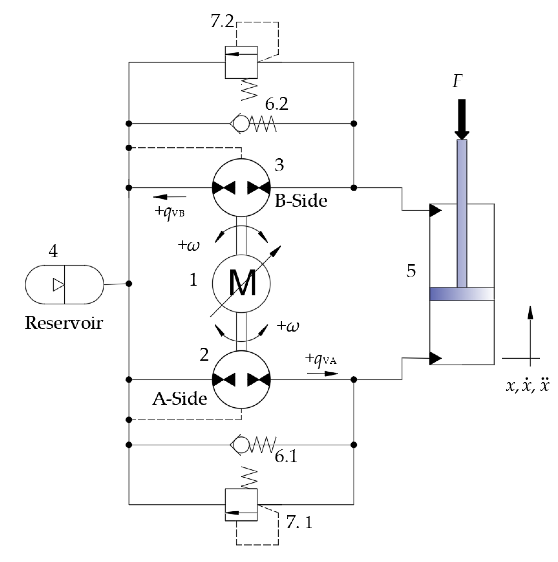
2. DDH and Modelling

2.1. DDH

Double-pump DDH uses a double fixed displacement pump driven by one variable speed electric motor to control a differential cylinder [5]. The schematics of the DDH system is shown in Figure 1. Parameters of the main components in the simulation are shown in

Table 1. Main parameters of the components.

No.	Component	Parameters	Value
1	Synchronous Torque Motor	Rated Torque [Nm]	4.5
		Rated Speed [rpm]	2500
2	A-Side Pump	Volumetric Displacement (DA) [cm3/rev]	13.03
3	B-Side Pump	Volumetric Displacement (DB) [cm3/rev]	9.35
4	Hydraulic Accumulator	Volume [L]	0.7
5	Cylinder	Dimensions [mm]	60/30*400

[5].

2.2. Modelling of DDH

This section describes the mathematical model of DDH. Compared to the pump-controlled system, the frequency of the electric motor is much higher. Hence, the dynamics of the electric motor are omitted.

The hydraulic cylinder flow continuity equation can be expressed by:

$$q_{\mathrm{A}}=A_{\mathrm{A}}\dot{x}+c_{\mathrm{i}}\left(p_{\mathrm{A}}-p_{\mathrm{B}}\right)+c_{\mathrm{e}}{p}_{\mathrm{A}}+\frac{V_{\mathrm{A}}}{{\beta }_e}{\dot{p}}_{\mathrm{A}},$$

(1)

$$q_{\mathrm{B}}=-A_{\mathrm{B}}\dot{x}+c_{\mathrm{i}}\left(p_{\mathrm{A}}-p_{\mathrm{B}}\right)-c_{\mathrm{e}}{p}_{\mathrm{B}}-\frac{V_{\mathrm{B}}}{{\beta }_e}{\dot{p}}_{\mathrm{B}},$$

(2)

$$V_{\mathrm{A}}=V_{0\mathrm{A}}+A_{\mathrm{A}}x,$$

(3)

$$V_{\mathrm{B}}=V_{0\mathrm{B}}-A_{\mathrm{B}}x,$$

(4)

where q_A and q_B are the flow rates into A and B chambers, A_A and A_B the effective cross-section areas of piston side and rod side, x the current position, c_i and c_e the internal and external leakage coefficients, V_A and V_B are the total volumes of the chamber A and chamber B, p_A and p_B are the pressures of the chamber A and chamber B and β_e is the effective bulk modulus. V_0A and V_0B are the dead volumes of A and B chambers.

The output flow of the pump is

$$q_{\mathrm{VA}}=n{D}_{\mathrm{A}}{\eta }_{\mathrm{A}},$$

(5)

$$q_{\mathrm{VB}}=n{D}_{\mathrm{B}}{\eta }_{\mathrm{B}},$$

(6)

where q_VA and q_VB are the flow rates of pump A and B, n is the motor speed; D_A and D_B are the flow rates of A-side and B-side pumps; η_A and η_B represent the volumetric efficiency of pump A and B.

The force balance equation of the piston is

$$p_{\mathrm{A}}{A}_{\mathrm{A}}-p_{\mathrm{B}}{A}_{\mathrm{B}}=M\ddot{x}+B\dot{x}+kx+F,$$

(7)

where M is the total mass of piston and load; F is the load force and disturbance acting on the piston; B viscous damping coefficient of the piston; k is the spring stiffness coefficient.

For simplification, the leakage part of the hydraulic cylinder is classified as disturbance and k = 0, and the state vector is defined as $x_0={\left[x_1,x_2,x_3\right]}^T={\left[x,\dot{x},\ddot{x}\right]}^T$.

The state space equation can be obtained from the double-pump DDH model:

$$\{\begin{array}{l}{\dot{x}}_1=x_2\hfill \\ {\dot{x}}_2=x_3\hfill \\ {\dot{x}}_3=r_1{x}_3+r_2{x}_2+b_{0}u+f\hfill \end{array}$$

(8)

$$r_1=-\frac{B}{M}, r_2=-\frac{{\beta }_e}{M}\left(\frac{A_{\mathrm{A}}{}^2}{V_{\mathrm{A}}}-\frac{A_{\mathrm{B}}{}^2}{V_{\mathrm{B}}}\right), b_0=\frac{{\beta }_e}{M}\left(\frac{A_{\mathrm{A}}{D}_{\mathrm{A}}{\eta }_{\mathrm{A}}}{V_{\mathrm{A}}}-\frac{A_{\mathrm{B}}{D}_{\mathrm{B}}{\eta }_{\mathrm{B}}}{V_{\mathrm{B}}}\right), f=-\frac{\dot{F}}{M},$$

where u is the DDH system input, η_A = η_B = 85%.

According to [5], mechanical parameters are shown as follows: M = 100 kg, β_e = 1.4 × 10⁹ (Pa), B = 100 N·s/m, hydraulic cylinder parameters V_0A = 55.8 × 10⁻⁶ m³, V_0B = 18.2 × 10⁻⁶ m³.

In actual conditions, there may be certain uncertainties in the load mass, leakage coefficient, bulk modulus, spring elastic coefficient, external load force, etc. The aim of this study is to design a controller to obtain an accurate position tracking under the condition of uncertain parameters being constant or time-varying.

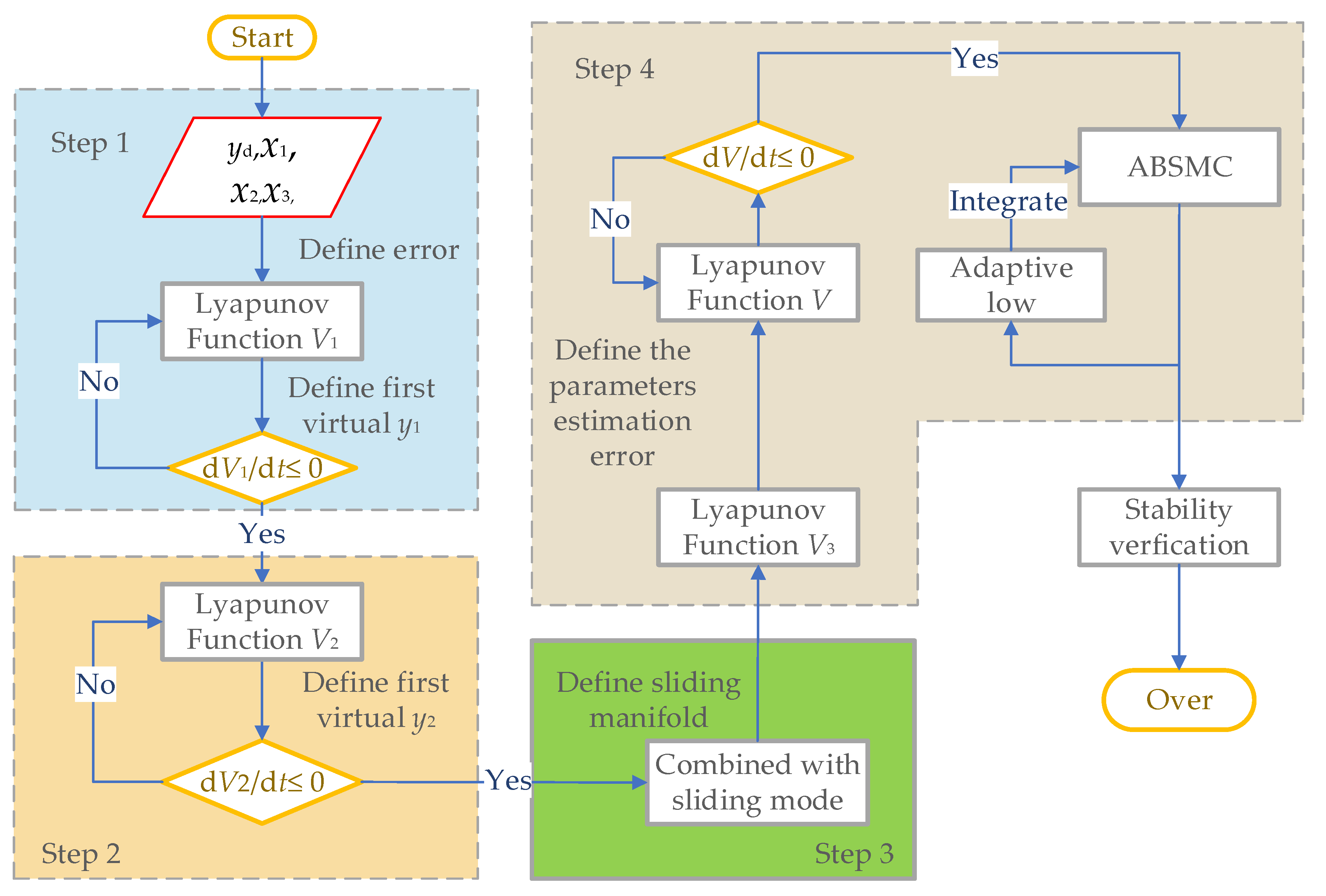
3. Design of ABSMC Controller

The backstepping design method, usually combined with Lyapunov-type adaptive law, comprehensively considers control law and adaptive law, so that the entire closed-loop system meets the expected dynamic and static performance requirements.

The backstepping control law requires accurate modelling information of the controlled object, and can not overcome the disturbance. However, the ABSMC requires neither the exact system model parameters nor certainty boundary of the uncertain parameters. The flowchart of the ABSMC is shown in Figure 2.

According to the simplified system model in Section 3, the DDH system can be expressed as a third-order linear system.

$$\{\begin{array}{l}{\dot{x}}_1=x_2\hfill \\ {\dot{x}}_2=x_3\hfill \\ {\dot{x}}_3=a_1{x}_1+a_2{x}_2+a_3{x}_3+bu+d\hfill \end{array} ,$$

(9)

where, a₁, a₂, a₃ and b are the unknown parameters, and d is an unknown disturbance.

3.1. Design of ABSMC and the Adaptive Law of Unknown Parameters

The ABSMC is designed for the system. In the controller, the adaptive law of unknown parameters is given by Lyapunov stability theorem, including the following steps.

Step 1: define the position tracking error.

All errors are defined as

$$\{\begin{array}{c}{e}_1=x_1-y_{\mathrm{d}}\\ e_2=x_2-y_1\\ e_3=x_3-y_2\end{array}.$$

(10)

where, y_d is the desired position, y₁ and y₂ are virtual control variables.

The derivative of Equation (10) gives

$$\{\begin{array}{l}{\dot{e}}_1=e_2+y_1-{\dot{y}}_{\mathrm{d}}\hfill \\ {\dot{e}}_2=e_2+y_2-{\dot{y}}_1\hfill \\ {\dot{e}}_3=a_1{x}_1+a_2{x}_2+a_3{x}_3+bu+d-{\dot{y}}_2\hfill \end{array}.$$

(11)

The Lyapunov function is chosen as

$$V_1=\frac{1}{2}{e}_1{}^2.$$

(12)

The derivative of Equation (12) gives

$${\dot{V}}_1=e_1{\dot{e}}_1=e_1\left(e_2+y_1-{\dot{y}}_{\mathrm{d}}\right).$$

(13)

The first virtual control is as follows

$$y_1=-k_1{e}_1+{\dot{y}}_{\mathrm{d}},$$

(14)

where k₁ > 0 is a design parameter.

Substituting Equation (14) into Equation (13) obtains

$${\dot{V}}_1=-k_1{e}_1{}^2+e_1{e}_2.$$

(15)

If $e_2=0$, then ${\dot{V}}_1\le 0$. Therefore, the backstepping algorithm is used again for the next step design.

Step 2: the Lyapunov function is chosen as

$$V_2=V_1+\frac{1}{2}{e}_2{}^2.$$

(16)

The derivative of Equation (16) gives

$${\dot{V}}_2={\dot{V}}_1+e_2{\dot{e}}_2=-k_1{e}_1{}^2+e_1{e}_2+e_2\left(e_3+y_2-{\dot{y}}_1\right).$$

(17)

The second virtual control is as follows

$$y_2=-k_2{e}_2+{\dot{y}}_1-e_1,$$

(18)

where k₁ > 0 is a design parameter.

Substituting Equation (18) into Equation (17) obtains

$${\dot{V}}_2=-k_1{e}_1{}^2-k_2{e}_2{}^2+e_2{e}_3.$$

(19)

If $e_3=0$, then we have ${\dot{V}}_2\le 0$. Therefore, the first two subsystems are stable.

Step 3: Combined with sliding model control.

Sliding mode control is used and the sliding manifold is defined as

$$s=c_1{e}_1+c_2{e}_2+e_3,$$

(20)

where c₁ and c₂ are the normal number.

The derivative of Equation (20) gives

$${\dot{s}}_2=c_1{\dot{e}}_1+c_2{\dot{e}}_2+{\dot{e}}_3=c_1\left(x_2-{\dot{y}}_d\right)+c_2\left(x_3-{\dot{y}}_1\right)+a_1{x}_1+a_2{x}_2+a_3{x}_3+bu+d-{\dot{y}}_2$$

(21)

Step 4: In order to avoid including the control variable u in the parameter adaptive law ${\widehat{\tau }}_4$ designed below—that is, to avoid loop nesting—the Lyapunov function is chosen as

$$V_3=V_2+\frac{1}{2b}{s}^2\ge 0.$$

(22)

The derivative of Equation (22) gives

$${\dot{V}}_3=-k_1{e}_1{}^2-k_2{e}_2{}^2+e_2{e}_3+s\left[\frac{c_1}{b}\left(x_2-{\dot{y}}_{\mathrm{d}}\right)+\frac{c_2}{b}\left(x_3-{\dot{y}}_1\right)\right]+s\left[\frac{a_1}{b}{x}_1+\frac{c_2}{b}{x}_2+\frac{c_2}{b}{x}_3+u+\frac{d}{b}-\frac{1}{b}{\dot{y}}_2\right].$$

(23)

Define ${\tau }_1=\frac{a_1}{,},{\tau }_2=\frac{a_2}{b},{\tau }_3=\frac{a_3}{b},{\tau }_4=\frac{d}{b}$, Equation (23) can be simplified as

$${\dot{V}}_3=-k_1{e}_1{}^2-k_2{e}_2{}^2+e_2{e}_3+s\left[\frac{c_1}{b}\left(x_2-{\dot{y}}_{\mathrm{d}}\right)+\frac{c_2}{b}\left(x_3-{\dot{y}}_1\right)+{\tau }_1{x}_1+{\tau }_2{x}_2+{\tau }_3{x}_3+u+{\tau }_4-\frac{1}{b}{\dot{y}}_2\right]$$

(24)

Define ${\tilde{\tau }}_1={\tau }_1-{\widehat{\tau }}_1,{\tilde{\tau }}_2={\tau }_2-{\widehat{\tau }}_2,{\tilde{\tau }}_3={\tau }_3-{\widehat{\tau }}_3,{\tilde{\tau }}_4={\tau }_4-{\widehat{\tau }}_4,{\tilde{a}}_4=a_4-{\widehat{a}}_4$ where, ${\widehat{\tau }}_1, {\widehat{\tau }}_2,{\widehat{\tau }}_3,{\widehat{\tau }}_4$ and ${\widehat{a}}_4$ are the estimated values of ${\tau }_1,{\tau }_2,{\tau }_3,{\tau }_4$ and $a_4$. ${\tilde{\tau }}_1,{\tilde{\tau }}_2,{\tilde{\tau }}_3,{\tilde{\tau }}_4$ and ${\tilde{a}}_4$ are the parameter estimation errors.

The Lyapunov function is chosen as

$$V=V_3+\frac{1}{2}{\lambda }_1{\tilde{\tau }}_1{}^2+\frac{1}{2}{\lambda }_2{\tilde{\tau }}_2{}^2+\frac{1}{2}{\lambda }_3{\tilde{\tau }}_3{}^2+\frac{1}{2}{\lambda }_4{\tilde{\tau }}_4{}^2+\frac{1}{2}{\lambda }_5{\tilde{a}}_4{}^2\ge 0,$$

(25)

where ${\lambda }_{\mathrm{i}}>0\left(i=1, 2, 3, 4, 5\right)$ is adaptive gain.

The derivative of Equation (25) gives

$$\begin{gathered} \dot{V}=-k_1{e}_1{}^2-k_2{e}_2{}^2+e_2{e}_3+s[c_1{a}_4(x_2-{\dot{y}}_d)+c_2{a}_4(x_3-{\dot{y}}_1)]+s[{\tau }_1{x}_1+{\tau }_2{x}_2+{\tau }_3{x}_3+ \\ u+{\tau }_4-a_4{\dot{y}}_2]+{\lambda }_1{\tilde{\tau }}_1(-{\dot{\hat{\tau }}}_1)+{\lambda }_2{\tilde{\tau }}_2(-{\dot{\hat{\tau }}}_2)+{\lambda }_3{\tilde{\tau }}_3(-{\dot{\hat{\tau }}}_3)+{\lambda }_4{\tilde{\tau }}_4(-{\dot{\hat{\tau }}}_4)+{\lambda }_5{\tilde{a}}_4(-{\dot{\hat{a}}}_4). \end{gathered}$$

(26)

The ABSMC is designed as follows

$$u=-c_1{\widehat{a}}_4\left(x_2-{\dot{y}}_{\mathrm{d}}\right)-c_2{\widehat{a}}_4\left(x_3-{\dot{y}}_1\right)-{\widehat{\tau }}_1{x}_1-{\widehat{\tau }}_2{x}_2-{\widehat{\tau }}_3{x}_3-{\widehat{\tau }}_4+{\widehat{a}}_4{\dot{y}}_2-h_{1}s-h_2\mathrm{sgn}\left(s\right),$$

(27)

where h₁ and h₂ are design parameters.

Substituting Equation (27) into Equation (26) obtains

$$\begin{gathered} \dot{V}=-k_1{e}_1{}^2-k_2{e}_2{}^2+e_2{e}_3-h_2{s}^2-h_{2}sgn(s)s+{\tilde{\tau }}_1(s{x}_1-{\lambda }_1{\dot{\hat{\tau }}}_1)+{\tilde{\tau }}_2(s{x}_2-{\lambda }_2{\dot{\hat{\tau }}}_2)+ \\ {\tilde{\tau }}_3(s{x}_3-{\lambda }_3{\dot{\hat{\tau }}}_3)+{\tilde{\tau }}_4(s{x}_4-{\lambda }_4{\dot{\hat{\tau }}}_4)+{\tilde{a}}_4[c_{1}s(x_2-{\dot{y}}_d)+c_{3}s(x_3-{\dot{y}}_1)-s{\dot{y}}_2-{\lambda }_5{\dot{\hat{a}}}_4]. \end{gathered}$$

(28)

The adaptive law of parameter variation is

$$\{\begin{array}{l}{\dot{\hat{\tau }}}_1=\frac{1}{{\lambda }_1}s{x}_1,{\dot{\hat{\tau }}}_2=\frac{1}{{\lambda }_2}s{x}_2,{\dot{\hat{\tau }}}_3=\frac{1}{{\lambda }_3}s{x}_3,{\dot{\hat{\tau }}}_4=\frac{1}{{\lambda }_4}s\hfill \\ {\dot{\hat{a}}}_4=\frac{1}{{\lambda }_5}s\left(c_1\left(x_2-{\dot{y}}_d\right)+c_2\left(x_3-{\dot{y}}_1\right)-{\dot{y}}_2\right)\hfill \end{array}$$

(29)

.

3.2. Stability Verification

The stability condition of the system can be obtained by analyzing the Lyapunov function.

The derivative of the Lapunov function of the system.

$$\dot{V}=-k_1{e}_1^2-k_2{e}_2^2+e_2{e}_3-h_1{s}^2-h_2\left|s\right|=-{\mathit{E}}^{\mathit{T}}\mathit{Q}\mathit{E}-h_2\left|s\right|,$$

(30)

where $\mathit{E}={\left[\begin{array}{ccc}{e}_1& e_2& e_3\end{array}\right]}^T,\mathit{Q}=\left[\begin{array}{ccc}{h}_1{c}_1^2+k_1& h_1{c}_1{c}_2& h_1{c}_1\\ h_1{c}_1{c}_2& h_1{c}_2^2+k_2& h_1{c}_2-\frac{1}{2}\\ h_1{c}_1& h_1{c}_2-\frac{1}{2}& h_1\end{array}\right]$.

For the DDH system, the controller (27) is designed, and its parameter adaptive law (29) is obtained. If appropriate controller parameters are selected, which should satisfy the following inequality

$$\{\begin{array}{l}{k}_1>0,k_2>0,h_1>0,h_2>0,c_1>0,c_2>0\hfill \\ k_1{k}_2+k_1{h}_1{c}_2{}^2+k_2{h}_1{c}_1{}^2>0\hfill \\ k_1{k}_2{h}_1+k_1{h}_1{c}_2-\left(k_1+h_1{c}_1{}^2\right)/4>0\hfill \end{array}.$$

(31)

Then, Q is a positive definite matrix, and then

$$\dot{V}=-{\mathit{E}}^{\mathit{T}}\mathit{Q}\mathit{E}-h_2\left|s\right|\le 0$$

(32)

.

Define $\mathit{G}={\mathit{E}}^T\mathit{Q}\mathit{E}$, and thus,

$$\dot{V}=-{\mathit{E}}^T\mathit{Q}\mathit{E}-h_2\left|s\right|\le -G,$$

(33)

$$\underset{t\to \infty }{\lim }\underset{0}{\overset{t}{{\displaystyle \int }}}Gdt\le \left[V\left(e_1\left(0\right),e_2\left(0\right),e_3\left(0\right)\right)-V\left(e_1(\infty ),e_2(\infty ),e_3(\infty )\right)\right].$$

(34)

Then, the position tracking error of the system is convergent, and the whole system is asymptotically stable.

According to Barbalat’s theorem,

$$\underset{t\to \infty }{\lim }G=0$$

(35)

.

Thus, it can be obtained that:

$$\underset{t\to \infty }{\lim }{e}_{\mathrm{i}}=0\left(i=1,2,3\right).$$

(36)

The position tracking error of the system is convergent. Similarly, it can be obtained that

$$\underset{t\to \infty }{\lim }s=0$$

(37)

.

Therefore, it can be concluded that the entire hydraulic position servo system is asymptotically stable, tends to the sliding surface within a limited period and moves along the desired trajectory.

4. Simulation and Analysis

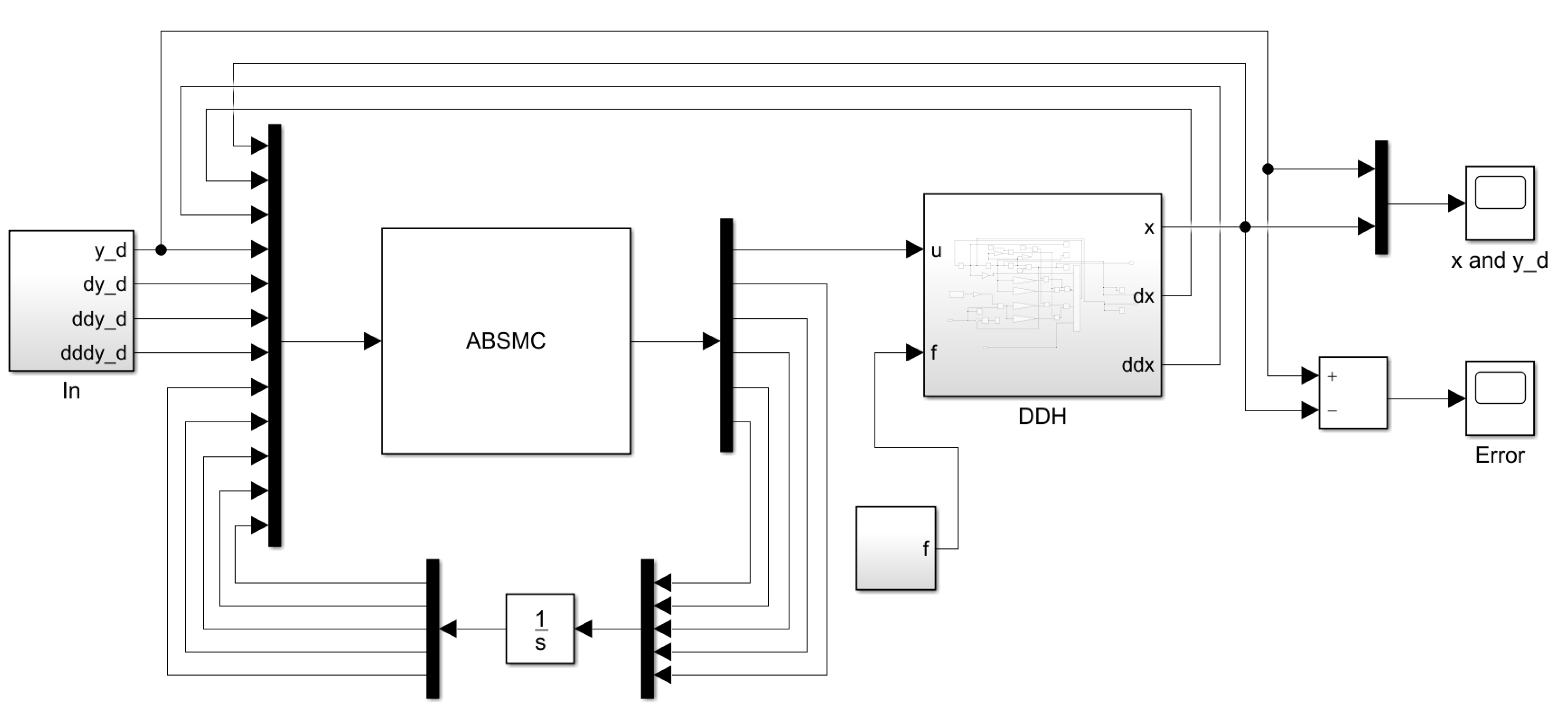
4.1. Simulation Model

The mathematic model of DDH in Section 2 and the control method in Section 3 were combined and used to create a Matlab/Simulink model of DDH system, as shown in Figure 3.

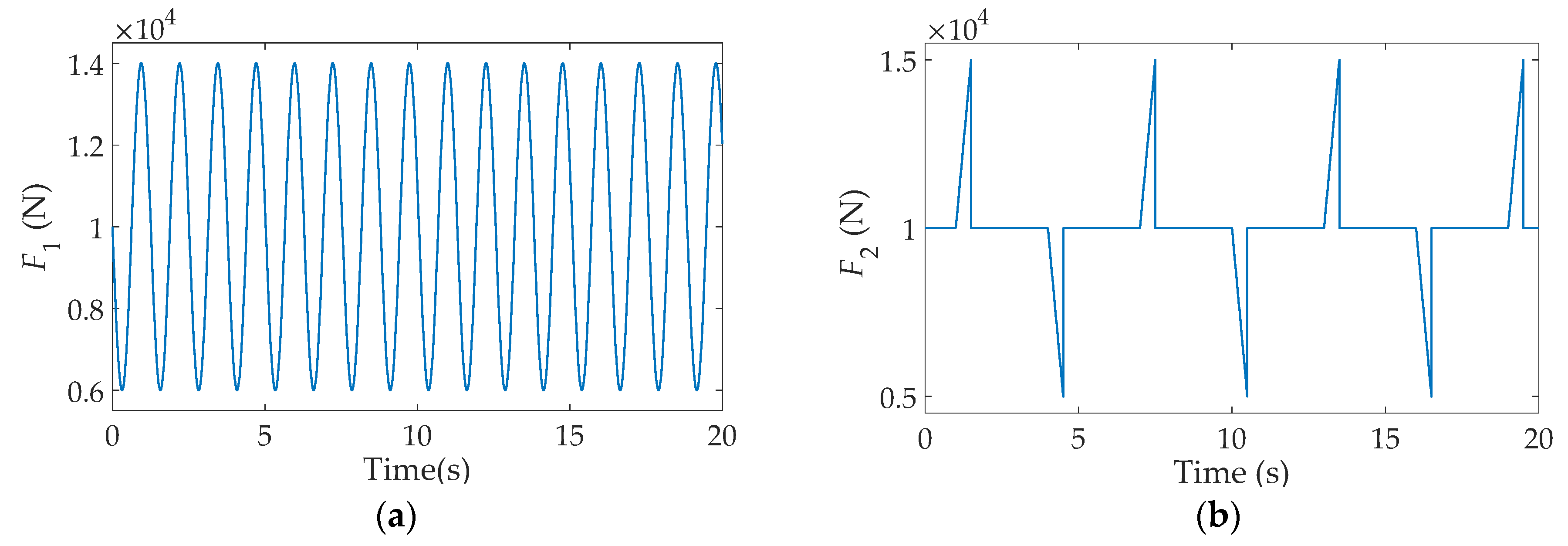
4.2. Load and Disturbance

In order to detect the antidisturbance ability of the controller, the sum of the load and disturbance force was set as F₁ = 10,000 − 4000cos(5t), as shown in Figure 4a. F₂ is a triangular signal, as shown in Figure 4b.

4.3. Simulation Analysis

A simple sinusoidal signal and a multifrequency sinusoidal signal were created as reference inputs to the model. Under the condition that Q is a positive definite matrix, appropriate parameters of the controller were selected as k₁ = 200, k₂ = 200, k₃ = 0.01, k₄ = 0.01, c₁ = 0.5, c₂ = 0.5, λ₁ = 1, λ₂ = 1, λ₃ = 0.5, λ₄ = 0.3, λ₅ = 100.

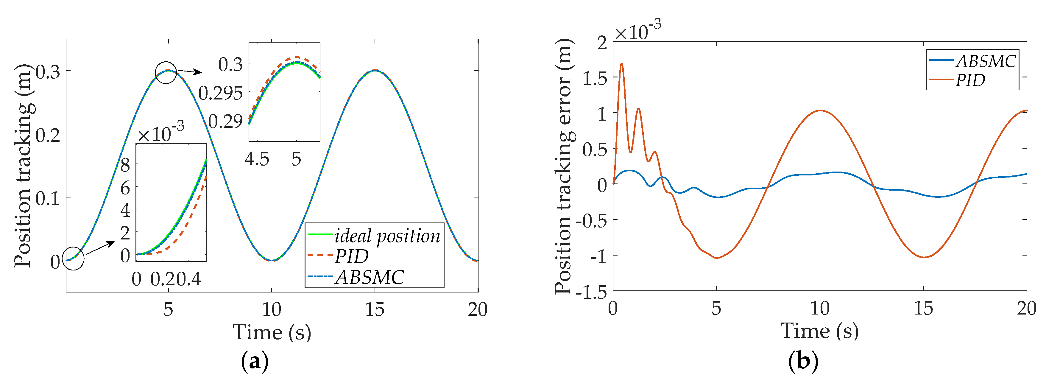
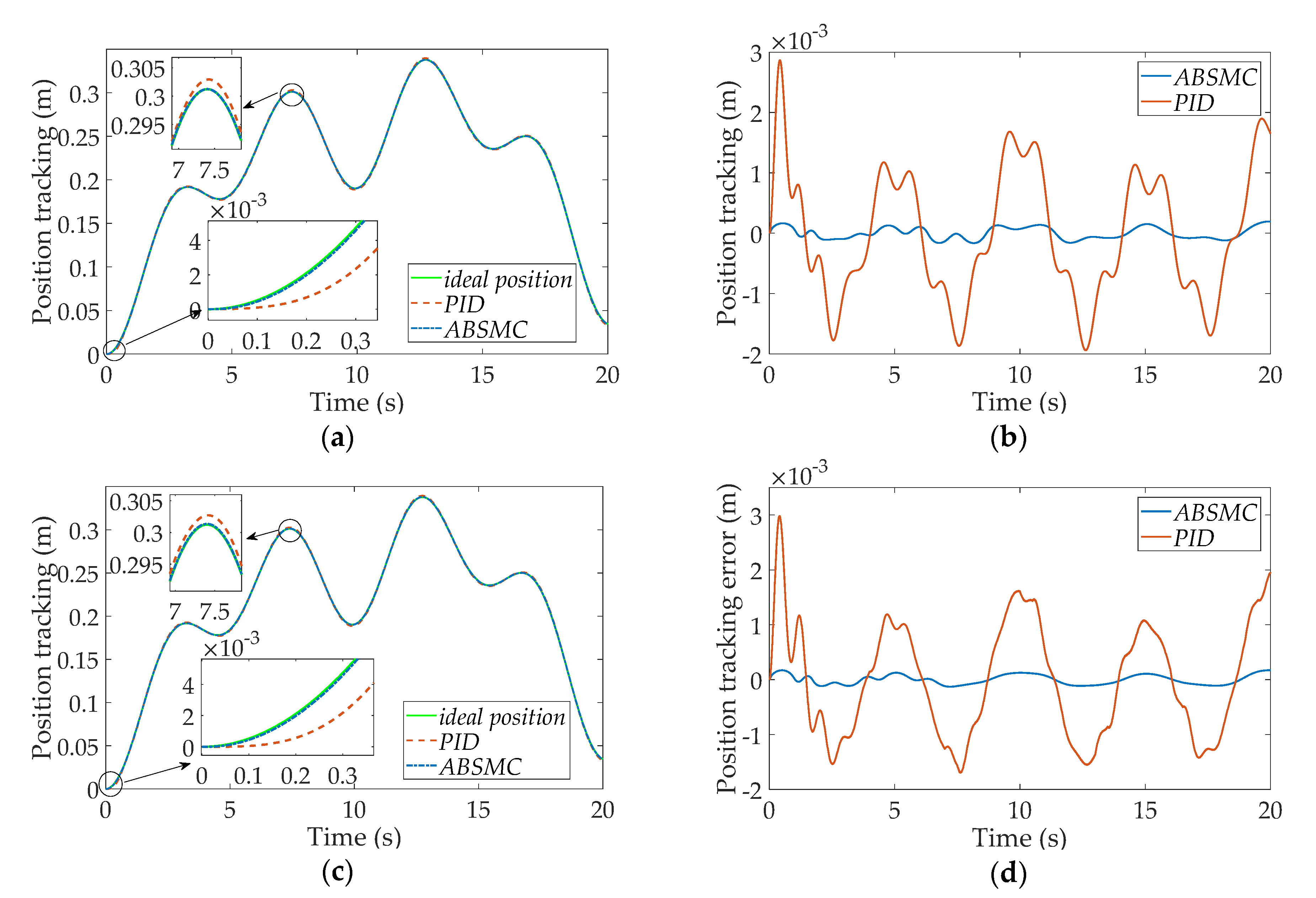
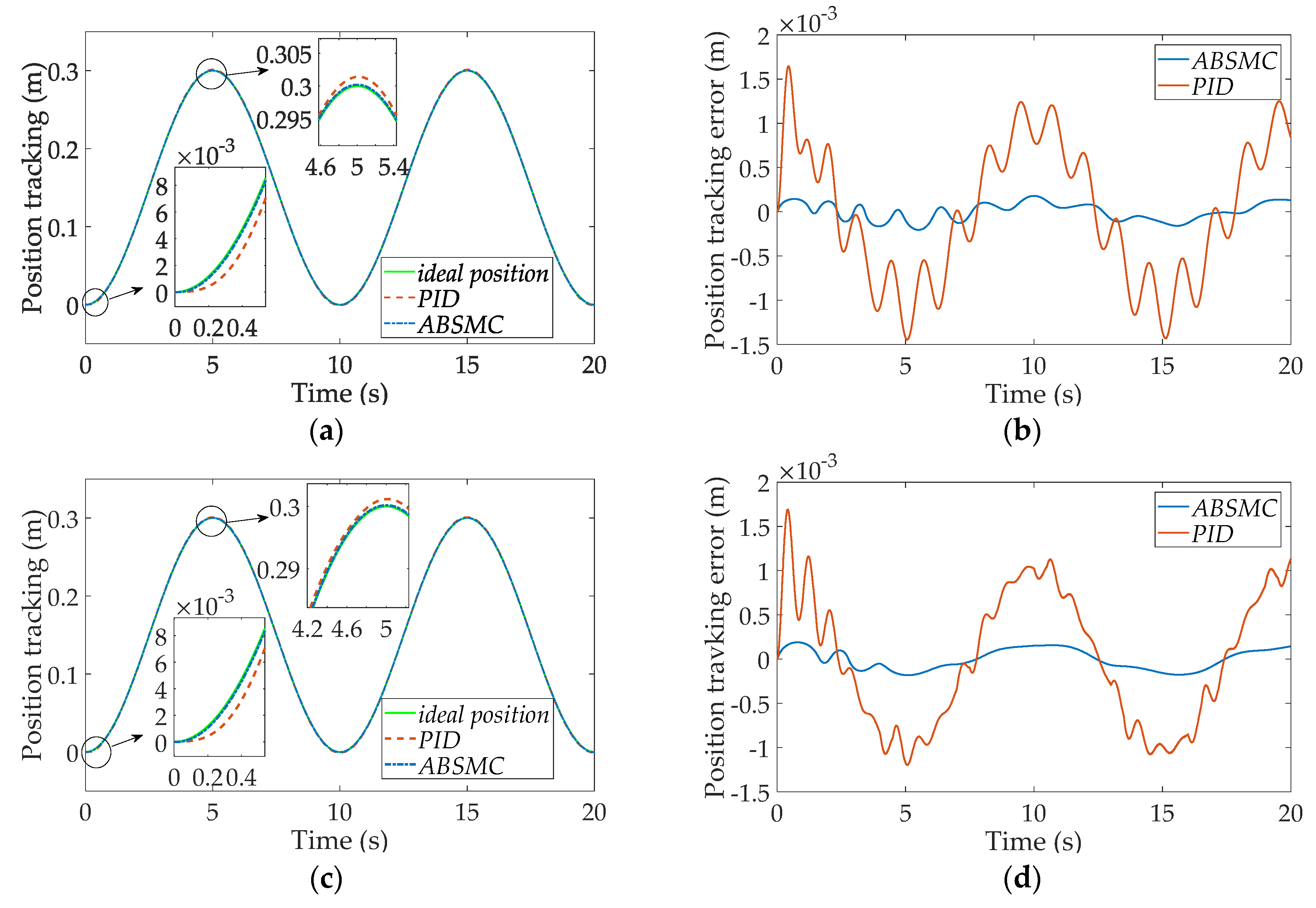
4.3.1. Simple Sinusoidal Signal

A simple sinusoidal single, $y_{\mathrm{d}}=0.15\sin (\frac{\pi }{5}t-\frac{\pi }{2})+0.15$, was used as the reference signal, and the tracking performances of the ABSMC and the general PID system were compared through simulation.

Without disturbance, the position tracking is shown in Figure 5a, and the position tracking error is shown in Figure 5b.

The simple sinusoidal curve was taken as the target displacement input to the DDH system, and the displacement output and error were observed under different disturbance. The simulation responses of the DDH position tracking with F₁ are shown in Figure 6a, and the position tracking error is shown in Figure 6b. Similarly, the simulation response of position tracking with F₂ is shown in Figure 6c, and the position tracking error results are shown in Figure 6d.

From the simulation results, the ABSMC position tracking error is much smaller compared with the traditional PID control. Moreover, the response speed is faster than that of the traditional PID control. With or without disturbance, the position tracking error of ABSMC basically remains unchanged, the error is small and it has strong antidisturbance capability and good robustness.

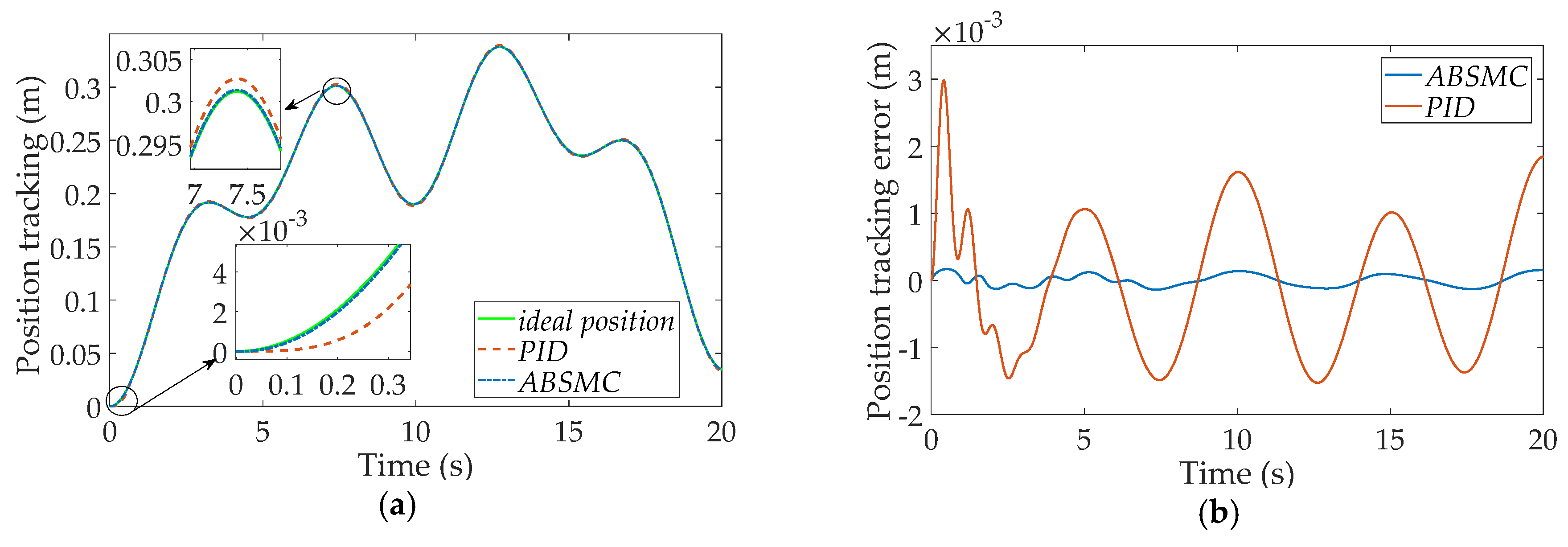
4.3.2. Multifrequency Sinusoidal Signal

Then, taking $y_{\mathrm{d}}=0.05\left[\sin \left(\frac{2\pi }{5}t-\frac{\pi }{2}\right)+\sin \left(\frac{\pi }{5}t-\frac{\pi }{2}\right)+\sin \left(\frac{\pi }{10}t-\frac{\pi }{2}\right)+\sin \left(\frac{2\pi }{25}t-\frac{\pi }{2}\right)+4\right]$ as the reference signal, the tracking performances of the ABSMC and the general PID system were compared through simulation.

Without disturbance, the simulation responses of position tracking are shown in Figure 7a. The position tracking error is shown in Figure 7b.

The multifrequency sinusoidal curve was taken as the desired displacement input to the DDH system, and the displacement output and error were observed under different disturbance. The simulation responses of DDH position tracking with F₁ are shown in Figure 8a, and the position tracking error is shown in Figure 8b. Similarly, the simulation response of position tracking with F₂ is shown in Figure 8c, and the position tracking error results are shown in Figure 8d.

The simulation results show that when the system is uncertain, with or without disturbance, the ABSMC is stable in the position tracking of the DDH, and the system output can track the position reference faster. Compared with the PID controller, the designed controller has a lower tracking error, faster response speed, better tracking performance and robustness.

5. Conclusions

In this paper, a controller adopting ABSMC was proposed for the double-pump DDH with unknown parameters, using an adaptive backstepping algorithm based on a linearized system model. According to the Lyapunov analysis and design, the ABSMC employs the appropriate parameter adaptive law to ensure the stability of the closed-loop system and the boundness of the parameters, which is supported by a theoretical proving. The proposed controller can address the problems of nonlinear characteristics, parameter uncertainty and uncertainty coefficient ahead of control input. A model was built, including the DDH and an ABSMC controller. Simulations were performed using two types of reference signal. The simulation results show that ABSMC can track the position accurately under varying load disturbances, regardless of simple or complex position reference. This control method can effectively address the problem that the designed control quantity and adaptive law are nested with each other due to the uncertainty coefficient ahead of the control input. It can effectively overcome the influence of the system’s nonlinearity and parameter uncertainty, has fast and accurate tracking and strong robustness to parameter changes.

Although the simulation results show that the ABSMC method can improve the position control accuracy of double-pump DDH, it lacks experimental data for comparison and verification. Therefore, the following research should establish a test bench and conduct experiment to validate the simulation results. In addition, the ABSMC method designed in this paper adopts the conventional design process which can be innovated in the future research.

References

1. Ketelsen, S.; Padovani, D.; Andersen, T.O.; Ebbesen, M.K.; Schmidt, L. Classification and Review of Pump-Controlled Differential Cylinder Drives. Energies 2019, 12, 1293. [Google Scholar] [CrossRef]
2. Kai, Z. Research on the Characteristics of Position Control Based on Variable Speed Pump Control System. Master’s Thesis, Shanghai Jiao Tong University, Shanghai, China, 2017. [Google Scholar]
3. Grabbel, J.; Ivantysynova, M. An Investigation of Swash Plate Control Concepts for Displacement Controlled Actuators. Int. J. Fluid Power 2005, 6, 19–36. [Google Scholar] [CrossRef]
4. Niraula, A.; Zhang, S.; Minav, T.; Pietola, M. Effect of Zonal Hydraulics on Energy Consumption and Boom Structure of a Micro-Excavator. Energies 2018, 11, 2088. [Google Scholar] [CrossRef]
5. Agostini, T.; Negri, V.D.; Minav, T.; Pietola, M. Effect of Energy Recovery on Efficiency in Electro-Hydrostatic Closed System for Differential Actuator. Actuators 2020, 9, 12. [Google Scholar] [CrossRef]
6. Altare, G.; Vacca, A. A Design Solution for Efficient and Compact Electro-hydraulic Actuators. Procedia Eng. 2015, 106, 8–16. [Google Scholar] [CrossRef]
7. Fu, S.; Wang, L.; Lin, T. Control of electric drive powertrain based on variable speed control in construction machinery. Autom. Constr. 2020, 119, 103281. [Google Scholar] [CrossRef]
8. Lin, T.; Lin, Y.; Ren, H.; Chen, H.; Chen, Q.; Li, Z. Development and key technologies of pure electric construction machinery. Renew. Sustain. Energy Rev. 2020, 132, 110080. [Google Scholar] [CrossRef]
9. Izzuddin, N.H.; Faudzi, A.M.A.; Johari, M.R.; Osman, K. System identification and predictive functional control for electro-hydraulic actuator system. In Proceedings of the IEEE International Symposium on Robotics & Intelligent Sensors, Langkawi, Malaysia, 18–20 October 2015; pp. 138–143. [Google Scholar]
10. Tony Thomas, A.; Parameshwaran, R.; Sathiyavathi, S.; Vimala Starbino, A. Improved Position Tracking Performance of Electro Hydraulic Actuator Using PID and Sliding Mode Controller. IETE J. Res. 2019, 1–13. [Google Scholar] [CrossRef]
11. Yao, J.; Deng, W. Active Disturbance Rejection Adaptive Control of Hydraulic Servo Systems. IEEE Trans. Ind. Electron. 2017, 64, 8023–8032. [Google Scholar] [CrossRef]
12. Guo, K.; Wei, J.; Tian, Q. Nonlinear adaptive position tracking of an electro-hydraulic actuator. Proc. Inst. Mech. Eng. C J. Mech. Eng. Sci. 2015, 229, 3252–3265. [Google Scholar] [CrossRef]
13. Alemu, A.E.; Fu, Y. Sliding mode control of electro-hydrostatic actuator based on extended state observer. In Proceedings of the 2017 29th Chinese Control And Decision Conference (CCDC), Chongqing, China, 28–30 May 2017; pp. 758–763. [Google Scholar]
14. Qi, H.; Liu, S.; Yang, R.; Yu, Y. Research on new intelligent pump control based on sliding mode variable structure control. In Proceedings of the 2017 IEEE International Conference on Mechatronics and Automation (ICMA), Takamatsu, Japan, 6–9 August 2017. [Google Scholar]
15. Miao, Z.; Cao, Y. Application of fuzzy PID controller for valveless hydraulic system driven by PMSM. J. Phys. Conf. Ser. 2019, 1168, 022010. [Google Scholar] [CrossRef]
16. Guo, J.; Ye, C.; Wu, G. Simulation and Research on Position Servo Control System of Opposite Vertex Hydraulic Cylinder based on Fuzzy Neural Network. In Proceedings of the 2019 IEEE International Conference on Mechatronics and Automation (ICMA), Tianjin, China, 4–7 August 2019; pp. 1139–1143. [Google Scholar]
17. Dong, H.; Gao, L.; Shen, P.; Li, X.; Lu, Y.; Dai, W. An interval type-2 fuzzy logic controller design method for hydraulic actuators of a human-like robot by using improved drone squadron optimization. Int. J. Adv. Robot. Syst. 2019, 16. [Google Scholar] [CrossRef]
18. Zad, H.S.; Ulasyar, A.; Zohaib, A. Robust Model Predictive Position Control of Direct Drive Electro-Hydraulic Servo System. In Proceedings of the 2016 International Conference on Intelligent Systems Engineering (ICISE), Islamabad, Pakistan, 15–17 January 2016. [Google Scholar]
19. Zhou, H.; Lao, L.; Chen, Y.; Yang, H. Discrete-time sliding mode control with an input filter for an electro-hydraulic actuator. IET Control Theory Appl. 2017, 11, 1333–1340. [Google Scholar] [CrossRef]
20. Järf, A. Flow Compensation Using Hydraulic Accumulator in Direct Driven Hydraulic Differential Cylinder Application and Effects on Energy Efficiency. Master’s Thesis, Aalto University, Espoo, Finland, 2016. [Google Scholar]
Figure 1. Schematics of direct driven hydraulics (DDH).
Proceedings 64 00001 g001
Figure 2. The flowchart of the adaptive backstepping sliding mode control (ABSMC).
Proceedings 64 00001 g002
Figure 3. The schematic diagram of the simulation model of the DDH control system.
Proceedings 64 00001 g003
Figure 4. Signal diagram of the sum of load and disturbance F: (a) load and disturbance F1; (b) load and disturbance F2.
Proceedings 64 00001 g004
Figure 5. Simple sinusoidal responses of double-pump DDH using ABSMC and proportional–integral–differential (PID) without disturbance: (a) position tracking without disturbance; (b) tracking error without disturbance.
Proceedings 64 00001 g005
Figure 6. Simple sinusoidal response of DDH using ABSMC and PID with disturbance: (a) position tracking with F1; (b) tracking error with F1; (c) position tracking with F2; (d) tracking error with F2.
Proceedings 64 00001 g006
Figure 7. Multifrequency sinusoidal response of DDH using ABSMC and PID without disturbance: (a) position tracking without disturbance; (b) tracking error without disturbance.
Proceedings 64 00001 g007
Figure 8. Multifrequency sinusoidal response of the DDH using ABSMC and PID with disturbance: (a) position tracking with F1; (b) tracking error with F1; (c) position tracking with F2; (d) tracking error with F2.
Proceedings 64 00001 g008