Allais–Ellsberg Convergent Markov–Network Game ^†

Abstract

Behavioral deviations from subjective expected utility theory, most famously captured by the Allais paradox and the Ellsberg paradox, have inspired extensive theoretical and experimental research into risk and ambiguity preferences. While the existing analyze these paradoxes independently, little work explores how such heterogeneously biased agents interact in networked strategic environments. Our paper fills this gap by modeling a convergent Markov–network game between Allais-type and Ellsberg-type players, each endowed with fully enriched loss matrices that reflect their distinct probabilistic and ambiguity attitudes. We define convergent priors as those inducing a spectral radius of <1 in iterated enriched matrices, ensuring iterative convergence under a matrix-based update rule. Players minimize their losses under these priors in each iteration, converging to an equilibrium where no further updates are feasible. We analyze this convergence under three learning regimes—homophily, heterophily, and type-neutral randomness—each defined via distinct neighborhood learning dynamics. To validate the equilibrium, we construct a risk-neutral measure by transforming losses into payoffs and derive a riskless rate of return representing players’ subjective indifference to risk. This applies risk-neutral pricing logic to behavioral matrices, which is novel. This framework unifies paradox-type decision makers within a networked Markovian environment (stochastic adjacency matrix), extending models of dynamic learning and providing a novel equilibrium characterization for heterogeneous, ambiguity-averse agents in structured interactions.

1. Game Setup

Behavioral violations of subjective expected utility theory, most notably the Allais paradox [1] and the Ellsberg paradox [2], have generated a large literature on risk and ambiguity preferences. Foundational models formalizing these deviations include rank-dependent and non-expected utility approaches [3] and ambiguity-averse preferences based on multiple priors [4]. Separately, a rich body of work studies learning and belief updating in networked environments [5,6,7]. However, little work integrates heterogeneous risk- and ambiguity-biased agents into strategic network settings. This paper contributes to this gap.

There are five players, three Ellsberg-type E₁, E₂, and E₃ and two Allais-type A₁ and A₂. Each player i has an enriched loss matrix L_i ∈ ℝ^2×2 whose rows correspond to states, θ ∈ {θ₁(good) and  θ₂ (bad)}, and whose columns correspond to actions a ∈ {a₁ (risky),  a₂ (safe)}. The baseline risk-neutral loss matrix is L = [l₁₁ l₁₂ l₂₁ l₂₂] = [−1 −1 1 1]. This corresponds to the loss of −1 in the good state under either action and the loss of +1 in the bad state under either action. The game introduces behavioral distortions through multiplicative weights. Machina’s [3] smooth ambiguity model modifies utility by probability-separable curvature. We introduce a matrix-superadditive analog that has multiplicative state-action weights—to be detailed in the full paper. For behavioral enrichment of losses, let W = (w_ij) and collect the multiplicative weights applied to each entry of L. Enriched losses are defined elementwise by L∗ = W ∘ L. Ellsberg-type players overweight ambiguity in the bad state. The weight matrix is W_E = [1 1 3 2], L_E∗ = [−1 −1 3 2]. Allais-type players overweight certainty in the good state. Their weight matrix is W_A = [2 2 1 1] and L_A∗ = [−2 −2  1  1]. Thus, E-type players become ambiguity averse in the bad state and A-type agents become certainty lovers in the good state.

The loss enrichment has implications for prior choice also. Let π∗(θ₁)_max denote the highest convergent prior for a player’s type—i.e., the largest prior probability assigned to state θ₁ for which the player’s loss matrix L yields spectral radius ρ(L) < 1. A loss matrix is thus fully enriched if the chosen prior is only the highest convergent prior (only decile priors are used here for simplicity). This makes sure, as a second-order condition on multiplicative state-action weights, that all of the subjective or empirical probability weights have been loaded upon, and transformed into, loss magnitudes. In theory, it must leave only purely unbiased priors to be chosen, such that any hesitation in choosing the highest convergent prior must force a revelation of some hidden probability or preference. So, the loss matrix for A has π∗(θ₁)_max ≈ 0.5, where π∗(θ₁)^A ∈ [0.1, 0.5] and for E π∗(θ₁)_max ≈ 0.9, where π∗(θ₁)^E ∈ [0.5, 0.9]. One can see how overweighting of good states (bad states) by Allais-type (Ellsberg-type) players is exactly penalized in the convergent prior set {π∗(θ₁)^A} ({π∗(θ₁)^E}). The fully enriched convergent expected loss vector is defined as

EL∗: = min_{π∗(θ1)max} {π∗(θ₁)_max[l₁₁, l₁₂] + (1 − π∗(θ₁)_max)[l₂₁, l₂₂]}.

Equivalently, EL∗ = EL(π∗(θ₁)_max), where ρ(L) < 1. This expresses the best-case (most favorable) convergent expected loss available to a player under its own feasible prior set. A player i ∈ {A, E} is declared the winner of the game M if and only if it most minimizes its fully enriched convergent expected loss vector: Winner = arg min _{i ∈ {A,E}} EL_i∗. Because losses are negative in our normalization, this means that the winner is the player whose enriched convergent expected loss is most negative.

The network structure of M is a row-stochastic Markovian adjacency matrix X ∈ ℝ^5×5. There are three scenarios built around neighborhood strength, or learning influence, r between any two players or two network nodes. For simplicity, there is no self-learning or self-neighborhood so {r_ii = r_jj = 0} ⇒ diag(X) = 0.

Scenario 1, Homophily:X is homophilous if r_A,A > r_A,E and r_E,E > r_A,E.

Scenario 2, Heterophily: X is heterophilous if r_A,A < r_A,E and r_E,E < r_A,E.

Scenario 3, Type-Neutral Random (TNR): X is TNR if each r is random.

Each iteration of X updates loss matrices by the linear Markov rule,

L_i^t+1 = ∑_j X_ij L_j^t 

This step does not use priors at all (it only needs the L matrices and X). Once a new iterated matrix is formed, the player selects a new highest convergent prior for reporting by scanning deciles and minimizing their EL* score—this is a post-processing selection based on the current L_i^t. That is, the transmission rule (how chosen π affects the next iteration) is as follows: once player i selects π_i∗^(t)_max, they transmit to neighbors the row-scaled matrix L_i^t~  =  diag(π_i∗^(t)_max, 1 −  π_i∗^(t)_max) L_i^t or equivalently, L_i^t~ = D(π_i∗^(t)_max) ∘ L_i^t in Hadamard form. The network update then uses L^~ as the input:

L_i^t+1 = ∑_j X_ij L_j^t~ 

Repeat: at iteration t + 1, each player computes its candidate π from the newly computed L_i^t+1, picks the highest convergent decile, transmits the scaled matrix to neighbors, and so on. The process stops when no player changes π (and/or when L converges).

2. Convergent Risk-Neutral Measure and Nash Equilibrium

Unique and Positive Risk-Neutral Measure: The following is only intended to show that under the unique and positive risk-neutral measure π⩛(θ) = {θ₁, θ₂} there is,

π⩛(θ₁)^A ≈ inf Δ*(Ω)^A 

π⩛(θ₁)^E ≈ sup Δ*(Ω)^E,

where Δ*(Ω) denotes the set of convergent priors.

The formal implications of this measure will be detailed in the full paper. Let there be two assets, a stock s, and a bond z, with a risk-free return of 0.05. There are two times t and u, where u has two states, θ₁ and θ₂ ∊ Ω, with number of assets = 2. At u, s has an empirical return probability of 10% and −5% for θ₁ and θ₂, respectively; so, the risky investment of USD 100 at t becomes USD 110 and USD 95 against a riskless USD 105 at u. The loss matrices are, for actions a₁ = invest in s and a₂ = invest in z. Take the risk-neutral baseline matrix L = [−1 −1 1 1] and incorporate the 10% and −5% for θ₁ and θ₂, respectively; we obtain L → E = [−1.1 −1.05 0.95 1.05] → E = [−1.1 −1.05 3 1], where E tends to a canonical fully enriched Ellsberg-type = [−1 −1 3 2]. So, the payoff matrix (of the loss matrix E) → [1.1 1.05 0.35 1.5], where riskless payoff a₂ = [1.05 1.5] is uninteresting. There is 1.1/0.35 = 3.14 in the second equation below for the case of E, which corresponds to the risky asset column a₁ = [−1, 3] ⇒ {−⅓ = −3 = (good state/bad state loss ratio) ≈ 1.1/0.35 = 3.14 (good state/bad state payoff ratio)} ⇒ risky payoff column a₁ = [1.1 0.35] for the loss matrix E. For L → A = [−1.1 −1.05 0.95 1.05] → A = [−2 −2 1 1] ⇒ a₁ = [−2 1] ⇒ {−2/1 = (good state/bad state loss ratio) ≈ 2/1 = 2 (good state/bad state payoff ratio)} ⇒ [2 1], so goes the second equation θ₁2 + θ₂ = 1.05 of the A case below. So, the payoff matrix (of the loss matrix A) → [2 1.3 1 1.05], where riskless payoff a₂ = [1.3 1.05] is again uninteresting.

θ₁1.05 + θ₂1.05 = 1.05    —E case

θ₁1.1 + θ₂0.35 = 1.05

{θ₁ = 0.93 ≈ 0.9 ≈ sup Δ*(Ω)^E, θ₂ = 0.06}| π⩛(θ)^E.

θ₁1.05 + θ₂1.05 = 1.05    —A case

θ₁2 + θ₂ = 1.05

{θ₁ = 0.05 ≈ 0.1 ≈ inf Δ*(Ω)^A, θ₂ = 0.95}| π⩛(θ)^A.

θ₁1.05 + θ₂1.05 = 1.05     —L case

θ₁ + θ₂ = 1.05

There is no measure for the risk-neutral loss matrix L, but every decile prior is convergent for L.

Under the calibrated enrichment weight, matrices W_E and W_A are used in the paper; the intersection between convergent and risk-neutral priors exists near the extremes of the decile grid used for the selection: Ellsberg-type preferences admit high admissible convergent priors (top decile), while Allais-type preferences admit low admissible convergent priors (bottom decile). Thus, when a unique positive risk-neutral measure exists and is used as the behavioral valuation kernel, it naturally maps to the top convergent decile for E-types (empirically close to 0.9, punishing undue risk aversion) and to the bottom convergent decile for A-types (empirically close to 0.1, penalizing undue love of certainty). The risk-neutral measure thus seals the lower convergent half for A-types into its limit case of the bottom decile and mutatis mutandis for E-types. So, this contextualizes iterative convergence under the spectral radius condition.

This is not a claim that 0.9 and 0.1 are universal; they are the model-consistent risk-neutral priors that emerge from our chosen W-calibration and the spectral stability criterion. Different enrichment weights, W, produce different risk-neutral priors. Note that this result—the risk-neutral priors’ smile from Allais to Ellsberg convergent priors—is owed to the second-order condition of choosing the highest convergent prior decile for the full enrichment of loss matrices.

Theorem 1 

(Nash Equilibrium). Let the game be M and let each player i hold a fully enriched loss matrix L_i∗ and updates by the linear network rule L^t+1 = X L^t with fixed row-stochastic network X, and at each iteration, each player selects a prior π only from the finite decile grid Δ(Ω) ≡ Π = {0.1,…,0.9}. Define for each player i the convergent set, such that

EL_i∗ = EL(π_i∗(θ₁)_max) where ρ(L_i*) < 1, π_i∗(θ₁)_max ∈ Δ*(Ω)_i

Suppose that W is positive and bounded so that the operator T(L) = X(W ∘ L) has a unique fixed point L∗. Then, the profile (π_i∗)_{{i =1, 5}} is a Nash equilibrium, such that no player can unilaterally choose a different prior other than π_i∗^(t)_max and obtain a strictly smaller fully enriched expected loss EL_i∗.

Proof: 

Under the assumptions, X is row-stochastic and W is positive and bounded; the map T(L) = X(W ∘ L) is a (uniform) contraction on a suitable compact set of bounded 2 × 2 matrices (one may normalize by a uniform bound on |W| and |L|). Hence, there exists a unique fixed point L∗ with L∗ = T(L∗). The intervening lemma on contraction necessity and sufficiency will be provided in the full paper. Feasible prior sets are closed intervals. For each player i, its convergent priors set Δ*(Ω)_i ⊂ Δ(Ω) is non-empty by construction (we assume that at least one decile satisfies ρ < 1), and in the decile grid it takes the form of an initial segment {0.1,…,π_{i max}}. So, π_{i max}* = maxΔ*(Ω)_i is well-defined.

Expected loss is affine in π (hence, there are extremal minimizers). That is, for a fixed L_i, each action’s expected loss EL_i^(a)(π) is affine in π. Consequently, the vector of action losses is minimized (or the criterion used to select EL*, e.g., the minimum across actions or the mean) over the discrete interval (with practically no loss of generality in the continuous case; more detail will be provided in the full version). Δ*(Ω)_i attains its minimum at an endpoint of that interval. By the game’s selection rule (highest convergent decile), the chosen endpoint is π_{i max}*.

For the essential Nash property of no profitable unilateral deviation, see the following. Suppose player i deviates to some other admissible prior π_i*~ ∈ Δ*(Ω)_i with π_i*~ ≠ π_{i max}*. Because the objective (EL*) is affine in π and we minimized it over Δ*(Ω)_i by selecting the endpoint π_{i max}*, we have EL_i∗(π_{i max}*) ≤ EL_i∗(π_i*~). Thus, the deviation cannot strictly decrease player i’s fully enriched convergent expected loss. (If multiple deciles tie at the minimum, the tie-breaking rule picks the highest decile; thus, any deviation to a lower decile cannot improve the objective.) Therefore, no player can strictly improve by unilaterally changing its prior from π_{i max}*, which means that (π_{i max}*) is a Nash equilibrium.

Corollary ⇒ Uniqueness under Strict Monotonicity: If, in addition, for each player i the function ELi(π) is strictly monotone on the admissible interval, as is the case (no ties at the minimizing endpoint), then the Nash equilibrium (π_{i max}*) is unique. □

3. Computational Results

The following are computations of the iterations for the above-mentioned three scenarios of the game.

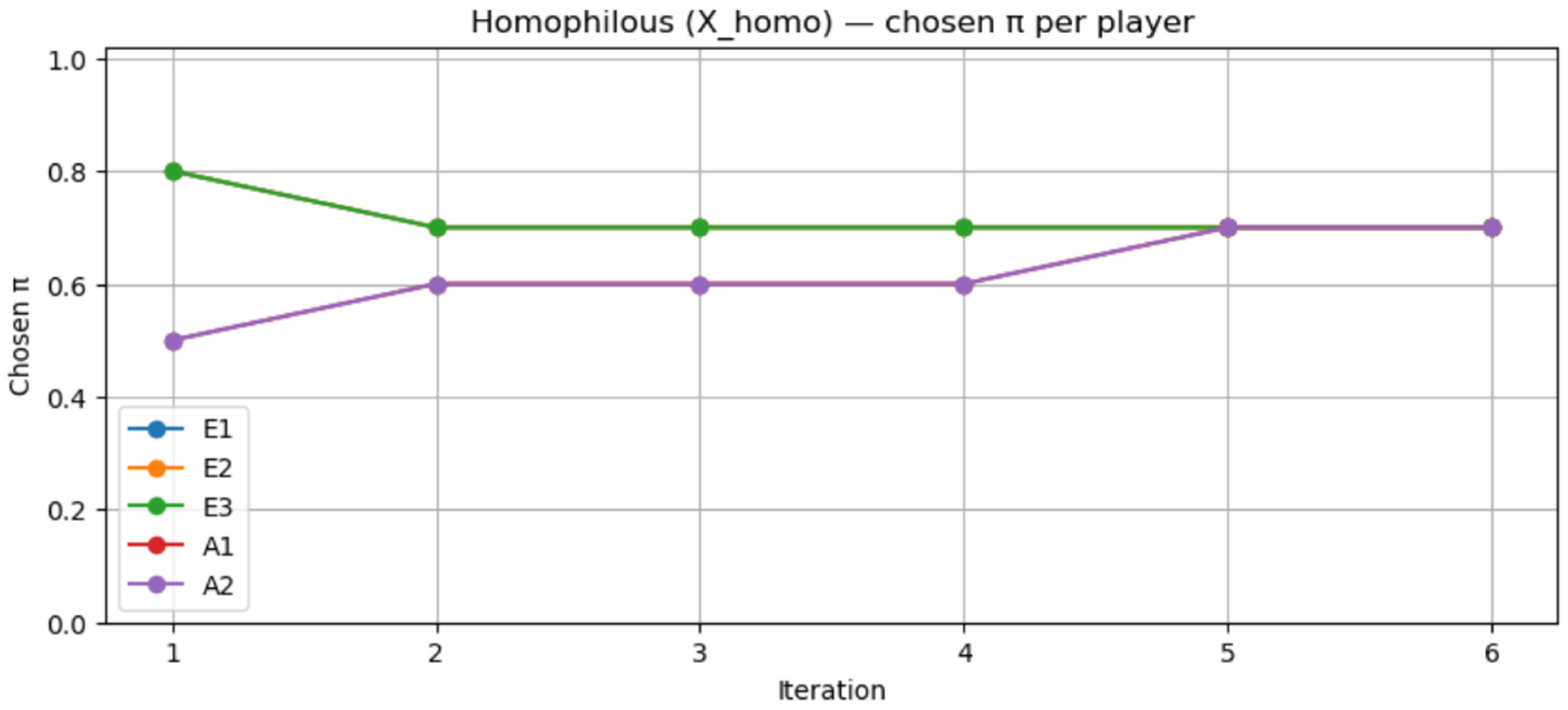
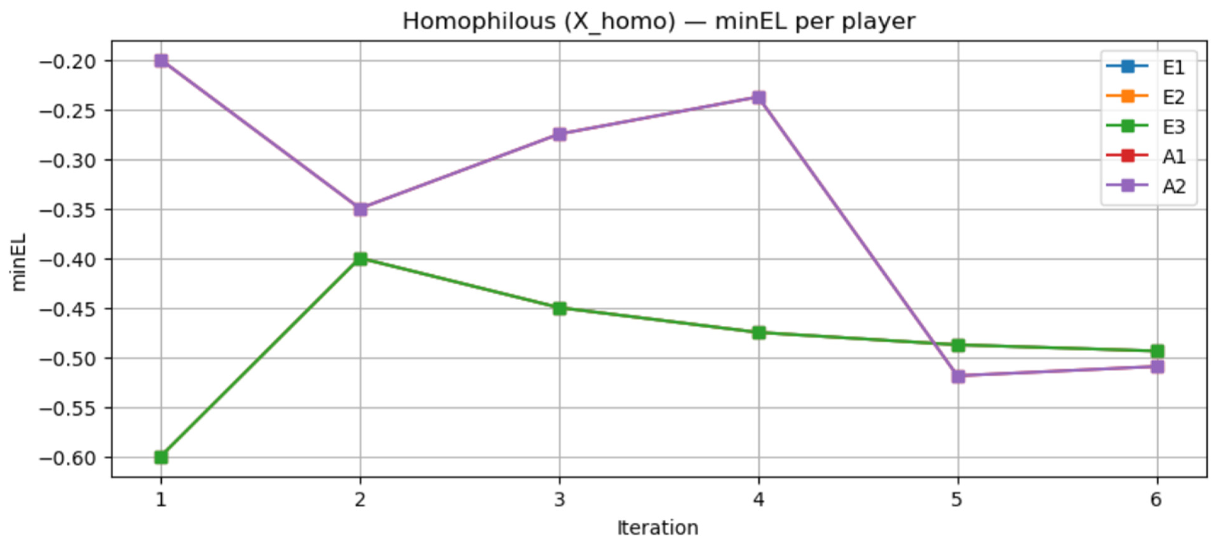
By the third iteration of homophily in Figure 1 and Figure 2, E-type players (green) win identically by minimizing the convergent expected loss the most as compared to A-type players (purple).

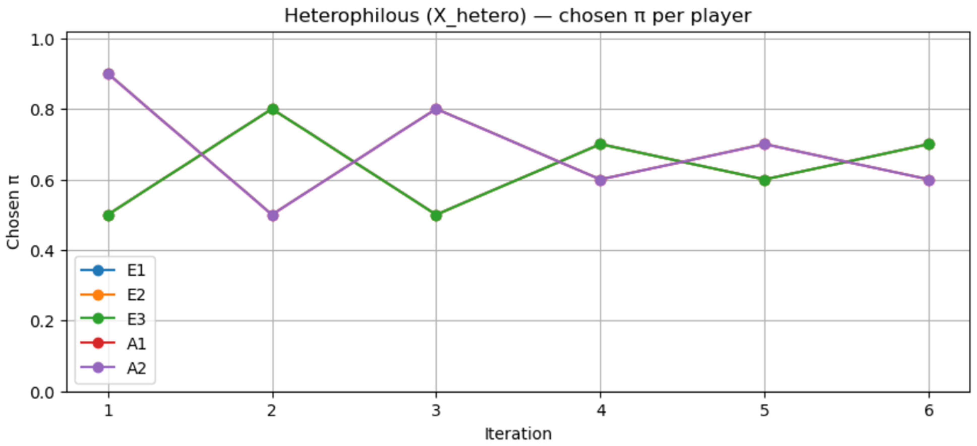
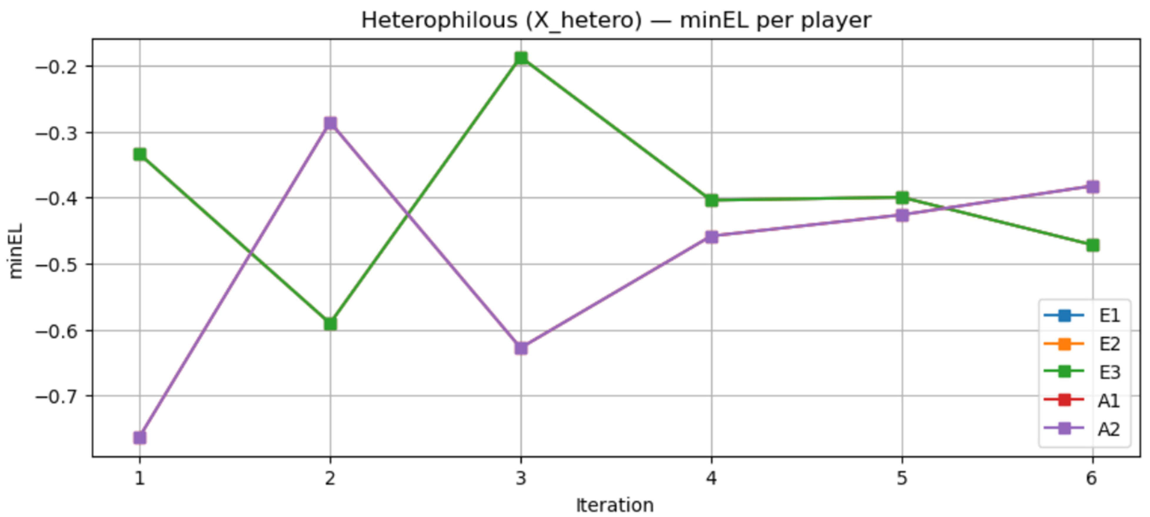
Heterophilous iterates in Figure 3 and Figure 4 produce fluctuations but converge quickly toward near-equal EL*s; E-type players (green) identically edge out slightly by iteration 3 as compared to A-type players (purple).

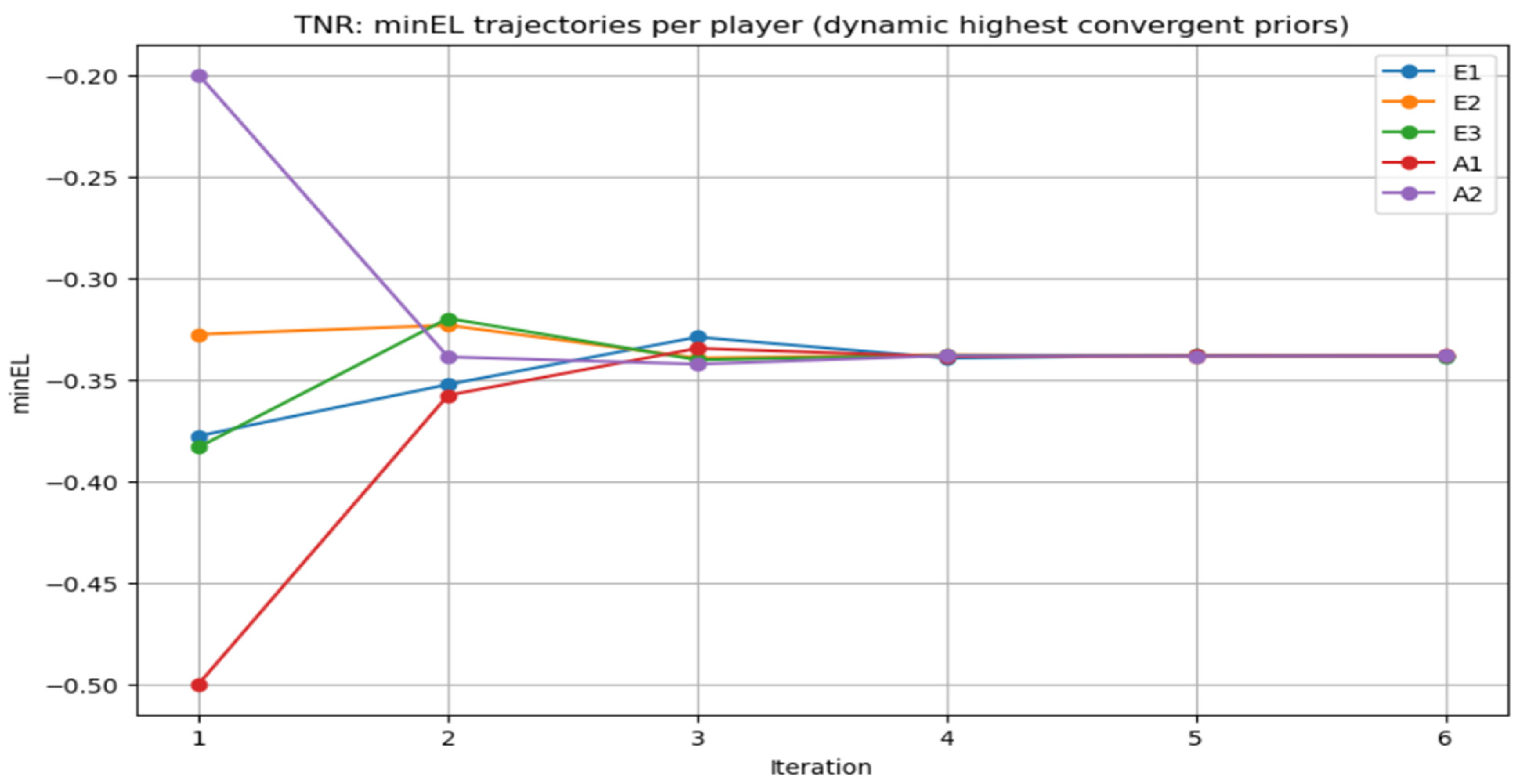
Type-neutral randomness in Figure 5 provides a full taste of the five-player stochastic network dynamics. Player A₂ wins uniquely by the third iteration, and the TNR scenario shows the fastest completion of learning with within-type differences.

Epistemic Value of the Game M: Consider a game ¬M with only one A and one E player. In the case of heterophily, after one iteration the matrices stop changing with same loss matrix {−1.5 −1.5 2 1.5}; in the Allais–Ellsberg convex combination case, under the transition matrix T = {0.5 0.5 0.5 0.5}, EL*_E = EL*_A = {−1.08 −1.14} with π*(θ₁)_max = 0.88.

An Application (Inverse Problems in Mean-Field Games): Let the mean-field operator be

$$\mathcal{T}(L): =\mathbf{\int }X(\mathit{\xi })[W(\mathit{\xi })\circ D({\pi }^{*}\left(L\right))\circ L(\mathit{\xi })]d\mathit{\xi }.$$

If $\rho \left(\mathcal{T}\right)<1$, then the mean-field game admits a unique equilibrium $L^{*}$ with ${\pi }^{*}\left(L^{*}\right),$ revealing true utility. X(ξ) is the mean-field interaction kernel (limit of the Markov network), aggregating how a player’s updated losses influence the game population; L(ξ) is the loss matrix of a representative player indexed by type $\xi$ (Allais or Ellsberg, possibly with heterogeneity).

Sketch of Proof. 

$\rho \left(\mathcal{T}\right)<1$ implies that $\mathcal{T}$ is a contraction; hence, $L_t\to L^{*}$. Since expected loss is affine in $\pi$, minimization over the convergent set selects its extreme (top for E, bottom for A), so any biased prior worsens convergence, and no deviation improves the inverse fit.