A Multi-Dimensional Feature Extraction Model Fusing Fractional-Order Fourier Transform and Convolutional Information

Abstract

In the field of deep learning, the traditional Vision Transformer (ViT) model has some limitations when dealing with local details and long-range dependencies; especially in the absence of sufficient training data, it is prone to overfitting. Structures such as retinal blood vessels and lesion boundaries have distinct fractal properties in medical images. The Fractional Convolution Vision Transformer (FCViT) model is proposed in this paper, which effectively compensates for the deficiency of ViT in local feature capture by fusing convolutional information. The ability to classify medical images is enhanced by analyzing frequency domain features using fractional-order Fourier transform and capturing global information through a self-attention mechanism. The three-branch architecture enables the model to fully understand the data from multiple perspectives, capturing both local details and global context, which in turn improves classification performance and generalization. The experimental results showed that the FCViT model achieved 93.52% accuracy, 93.32% precision, 92.79% recall, and a 93.04% F1-score on the standardized fundus glaucoma dataset. The accuracy on the Harvard Dataverse-V1 dataset reached 94.21%, with a precision of 93.73%, recall of 93.67%, and F1-score of 93.68%. The FCViT model achieves significant performance gains on a variety of neural network architectures and tasks with different source datasets, demonstrating its effectiveness and utility in the field of deep learning.

1. Introduction

Deep learning has made breakthroughs in recent years in the fields of computer vision, natural language processing [1], etc., especially based on convolutional neural network [2] (CNN) and recurrent neural network [3] (RNN) models, which have shown excellent performance in tasks such as image classification, target detection, and speech recognition. However, traditional network architectures still have limitations in dealing with long-range dependencies, computational parallelization, and global information modeling.

The Transformer model has revolutionized the research paradigm of deep learning since it was proposed by Vaswani [4] et al. in 2017. It escapes from the sequential computation limitation of RNNs, relies on the self-attention mechanism [5] to capture global dependencies, and shows great potential in areas such as language modeling, computer vision, and time series analysis. Especially in the field of natural language processing, the Transformer model became the core architecture of pre-trained language models such as BERT [6] and GPT [7]. In the field of computer vision, ViT further validates the feasibility of the self-attention mechanism in image classification tasks [8]. ViT has achieved considerable success in vision tasks; however, it still faces some challenges. For instance, ViT directly computes global self-attention on the entire image, which results in excessive computational overhead on high-resolution images. The ViT model is distinguished by its absence of local inductive bias in comparison to CNNs, a characteristic that limits its generalizability when confronted with limited datasets. In order to enhance the adaptability of Transformer in the field of computer vision, hierarchical and window-based improvement schemes have been proposed. The most representative of these is the Swin Transformer model [9]. The success of the Swin Transformer model in visual tasks further demonstrates the potential of the Transformer model in computer vision. Furthermore, enhancements have been made to the Swin Transformer model. Jianwei Yang [10] et al. proposed the Focal Transformer model as an evolution of the Swin Transformer model. This model introduces a hierarchical attention mechanism, enhancing the model’s local and global feature modeling capabilities and improving the Transformer model’s performance on high-resolution visual tasks. Ali Hatamizadeh [11] et al. combined the hierarchical window attention mechanism of the Swin Transformer model with the 3D medical image segmentation task to significantly improve the segmentation accuracy and computational efficiency. The first introduction of Transformer to target detection was the Detection Transformer [12] (DETR) proposed by Carion et al. This model realizes an end-to-end detection framework, which is free from the traditional Anchor mechanism and hand-designed post-processing steps. The DETR model proved the effectiveness of Transformer in target detection tasks. Shiyang Li [13] et al. demonstrated the advantages of Transformer on time series prediction tasks by utilizing the self-attention mechanism to capture long-range dependencies. Transformer has demonstrated strong performance in sequential and visual tasks, but its ability to model structured data is still limited, and it is difficult to directly capture the topological relationships between nodes. Ying [14] and others proposed the Graphormer model, which enhances Transformer’s perception of graph data by introducing structural coding, and achieved significant improvements in molecular modeling, social network analysis, and other tasks.

For semantic segmentation tasks, Strudel [15] et al. proposed the Segmenter model and further explored the application of the Transformer model in dense prediction tasks. The Segmenter model uses a pure Transformer structure to classify images pixel by pixel, achieving efficient and accurate semantic segmentation. He [16] et al. proposed the masked autoencoder (MAE) strategy, which achieves efficient self-supervised learning by masking most of the image patches and reconstructing only the missing portions. The MAE strategy proves that masked autoencoders can be used as a scalable visual learning method and further promotes the development of Transformer in the field of computer vision. In further exploring a more effective pre-training method for ViT, Bao [17] et al. proposed the BEiT model, which draws on the Masked Image Modeling strategy of the BERT model to allow the Transformer to learn richer visual representations by recovering masked image blocks. With the successful application of Transformer in several fields, more complex non-Euclidean spaces are taken as a new direction to explore. Fein-Ashley [18] et al. proposed a hybrid architecture of a Hyperbolic Vision Transformer by combining hyperbolic and Euclidean geometries, which efficiently captures hierarchical structures in the image data and the localized relationships in image data. In the field of medical image processing, ViT also shows excellent performance. In the task of breast cancer pathology image classification, the ViT-DeiT [19] model is able to effectively capture global features and improve the classification performance by combining the ViT model and Data-efficient Image Transformer model. Koushik Sivarama Krishnan [20] and others demonstrated the potential of Transformer in medical image classification by applying it to the task of COVID-19 [21] detection in chest X-ray images by utilizing the ability of the ViT model to capture global features.

Although some studies have applied fractional Fourier transform (FrFT) to neural network structures to enhance the frequency domain modeling ability of models, such as Wu et al. [22] combining FrFT with convolutional neural networks for robust face recognition tasks, and Barshan et al. [23] using FrFT as a preprocessing method for neural networks for object recognition, these methods typically rely on fixed transformation orders and lack adaptive modeling capabilities for task-specific frequency domain projections.

ViT uses a global self-attention mechanism that is capable of capturing long-range dependencies and lacks the local inductive bias inherent in CNNs when dealing with local features (like edges, textures, and so on). To address the above limitations, the following improvements are proposed by this study:

(1)

A Fractional-Order Fourier Transform (FrFT) module based on the Chirp-Z algorithm approximation of the learnable order is introduced. The fractional-order Fourier transform module can provide more flexible frequency domain sensing capabilities. By introducing a learnable parameter to control the “order” of the transformation, the model can automatically adjust the optimal degree of frequency domain projection during the training process. This approach enhances the model’s ability to perceive multi-scale and non-stationary signals, effectively improves the expressive power of feature extraction, and is especially suitable for dealing with data scenarios with complex pattern distributions.

(2)

A custom convolution module is incorporated to extract local features using convolutional layers. The custom convolution module can effectively capture texture and shape changes within a localized region, which is especially important for processing images or spatial data.

(3)

Combining three different types of feature extraction methods (attention mechanism, convolutional network, and fractional-order Fourier transform) to extract features from input data from different perspectives, the model integrates different information from the three branches. The three-branch fusion approach not only preserves the characteristics of each branch, but also combines their strengths, and improves the model’s ability to handle complex data.

2. Fractional Convolution Vision Transformer Model

2.1. Vision Transformer

Vision Transformer (ViT) is an image classification model based on the Transformer structure, proposed by Dosovitskiy et al. It breaks away from the dominance of traditional convolutional neural networks in computer vision tasks. ViT employs Transformer for global modeling, which captures long-range dependencies of images through a self-attentive mechanism. The Vision Transformer model architecture is shown in Figure 1.

ViT segments the input image into fixed-size patches, treating each patch as a “token” to be processed. Assuming that the input image is $X\in R^{H\times W\times C}$, where H,W,C denote the height, width, and number of channels of the image, respectively, it is first segmented with each patch size P× P, and the number of patches N generated is calculated as shown in Equation (1):

$$N={\displaystyle \frac{H}{P}}\cdot {\displaystyle \frac{W}{P}}$$

(1)

Each patch is spread and mapped to a D-dimensional embedding space, computed as shown in Equation (2):

$$z_i=W_e\cdot x_i+b,i=1,2,\dots ,N$$

(2)

where $z_i$ denotes the embedding vector of the $i$th image patch after linear projection; $x_i$ is the patch after spreading; $W_e$ is the linear transformation matrix; b is the bias term; and N denotes the number of patches. The final embedding sequence $Z\in R^{N\times D}$ is obtained.

ViT introduces a trainable category token $Z_0$ (a randomly initialized and learnable classification token), similar to BERT’s [CLS](Classification) token, together with a fixed positional encoding E, computed as shown in Equation (3):

$$Z_0=[z_o;z_1+E_1;z_2+E_2;\dots ;z_N+E_N]$$

(3)

where $Z_0$ denotes the token sequence of the input Transformer.

The backbone structure of ViT uses a standard Transformer encoder, which consists of multiple layers stacked on top of each other, each of which consists of three main key modules: multi-head self-attention, a feed-forward network (FFN), and LayerNorm with enhanced gradient propagation through residual connectivity.

ViT employs a multi-head mechanism, whereby multiple attention heads are computed in parallel. Multi-head self-attention is utilized to compute the global relationship between input tokens, thereby enhancing feature expression. The multi-head self-attention calculation formula is shown in Equation (4):

$$Attention(Q,K,V)=softmax({\displaystyle \frac{Q{K}^T}{\sqrt{d_k}}})V$$

(4)

where Q,K,V are Query, Key, and Value, respectively, generated from the input Z by different projection matrices; and $d_k$ is the dimension of the attention header, softmax normalized to compute the weighted sum to obtain the global context information.

The feed-forward network consists of a two-layer fully connected network, which usually contains the GELU (Gaussian Error Linear Unit) activation function, and the feed-forward network layer is calculated as shown in Equation (5):

$$FFN(x)=\sigma (W_{1}x+b_1)W_2+b_2$$

(5)

where $W_1,W_2$ is the weight matrix; $b_1,b_2$ is the bias term; and $\sigma (\cdot )$ is the GELU activation function.

2.2. Fractional-Order Fourier Transform Module

Fourier transform is a mathematical tool to convert a signal from the time domain to the frequency domain, and its core idea is to decompose a complex signal into a superposition of multiple sinusoids of different frequencies. Through this decomposition, the intensity and phase distribution of each frequency component of the signal can be clearly analyzed, thus revealing the frequency domain characteristics of the signal.

In order to realize efficient and microscopic fractional-order Fourier transform, the fractional-order Fourier transform (FrFT) implementation based on the approximation of the Chirp-Z algorithm is adopted in this study, which is approximated in the form of modulated signals, FFTs, and remodulation to obtain the effect of FrFT. The approximate fractional-order Fourier transform formula is shown in Equation (6):

$$F_{\alpha }(x(t))\approx Chirp(t)\cdot F[x(t)\cdot Chirp(t)]$$

(6)

where α is the order parameter of the fractional-order Fourier transform, which controls the degree of transformation, and is equivalent to the original signal when α = 0, to the standard Fourier transform when α = 1, and to the abelian transform of the FrFT when $\alpha \in (0,1)$; $F_{\alpha }$ denotes the order of the FrFT; Chirp denotes the exponential modulation kernel; t is the time (or sequence) index; and $x\left(t\right)$ is the original signal (time domain function).

The specific implementation process is to construct an exponential modulation function (Chirp kernel) for each feature channel. The input signal is first multiplied with the Chirp kernel to complete the exponential weighting of the time domain signal, achieving the purpose of Chirp modulation. The Chirp pre-modulation formula is shown in Equation (7):

$$x_1(t)=x(t)\cdot e^{-j\pi t^2\tan \varphi /N}$$

(7)

where $\varphi$ represents the FrFT rotation angle; $\tan \varphi$ represents the “degree of curvature” for controlling modulation; and $x_1(t)$ represents the pre-modulated Chirp signal.

The modulated signal is input into the standard Fast Fourier Transform (FFT) to obtain the initial spectrum, as shown in Equation (8):

$$X_1(f)=F[x_1(t)]$$

(8)

where $F[\cdot ]$ represents the Fourier transform operation.

The frequency spectrum and Chirp core are multiplied again to obtain an approximate fractional frequency domain result to achieve inverse modulation processing. The Chirp post-modulation formula is shown in Equation (9):

$$X_{\alpha }(u)=X_1(f)\cdot e^{-j\pi u^2\tan \varphi /N}$$

(9)

where $u$ represents the frequency domain index.

The Chirp-Z method is a strict transformation of FrFT that includes frequency scaling and phase compensation. It uses a discrete form to approximate the integral definition of continuous FrFT. FFT can only handle discrete sequences and cannot represent true continuous integration. Overall, it is a numerical approximation.

Fast Fourier Transform (FFT) is an efficient algorithm for discrete Fourier transform which is able to quickly convert time domain signals into frequency domain representations, greatly reducing computational complexity. FFT is able to efficiently extract the key frequency features of signals by converting time domain signals into frequency domain representations. Assuming that the last dimension of the input tensor x has N elements, the FFT output $x_k$ is computed as shown in Equation (10) for any slice on that dimension (other dimensions are fixed):

$$X_k={\displaystyle \sum _{n=0}^{N-1}{x}_n}\cdot e^{-i{\displaystyle \frac{2\pi }{N}}kn},k=0,1,\dots ,N-1$$

(10)

where $x_n$ is the nth element of the last dimension of the input tensor; $X_k$ is the kth complex component of the last dimension of the output tensor; i is an imaginary unit; and $e^{-i{\displaystyle \frac{2\pi }{N}}kn}$ is the rotation factor.

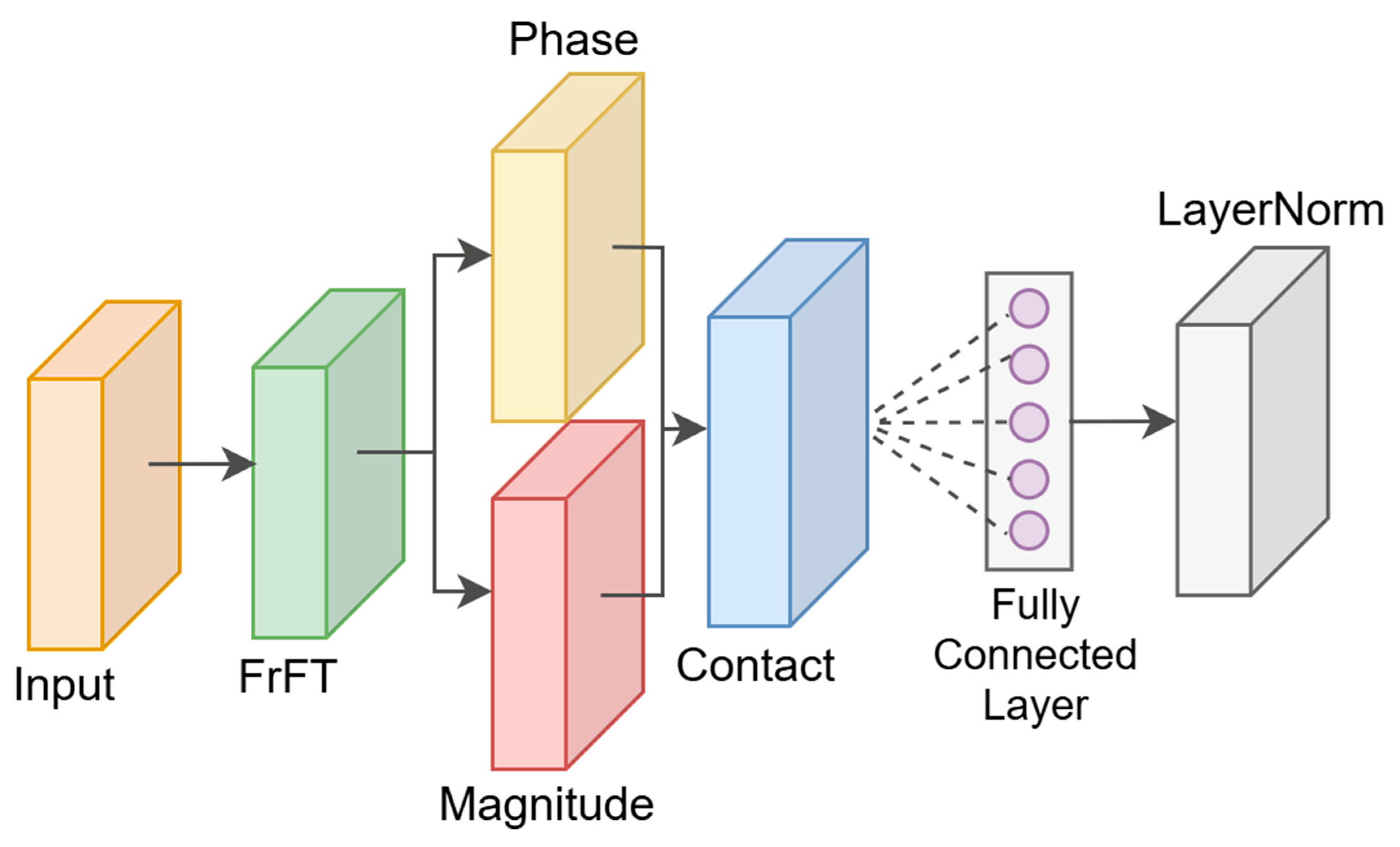
Since the input data are three-dimensional tensors at this point, FFT is performed on each 1 × 768 matrix along the direction of the columns. The FFT operation is illustrated in Figure 2.

The fractional-order Fourier module designs the order parameter α of the FrFT as a learnable parameter, which is dynamically optimized during the training process by gradient backpropagation. To prevent α from crossing the boundary, a sigmoid function is used to constrain it in the (0,1) interval and further mapped to the rotation angle $\varphi \in (0,{\displaystyle \frac{\pi }{2}})$ to control the degree of signal transformation in the complex plane. The implementation of FrFT is based on the Chirp-Z Transform algorithm. The Chirp-Z algorithm allows frequency sampling on non-unit-circle paths. The specific formulation of the Chirp-Z algorithm is shown in Equation (11):

$$X_k={\displaystyle \sum _{n=0}^{N-1}{x}_n}\cdot {z_k}^{-n},z_k=A\cdot W^{-k},k=0,1,\dots ,M-1$$

(11)

where A is the starting point of the complex plane; W is the rotation factor of each step; $z_k$ defines an arbitrary sampling path; $x_n$ denotes the nth sampling point of the original discrete signal; and $x_k$ denotes the kth output spectral value after the transformation of the Chirp-Z algorithm.

The fractional-order Fourier module maps the input sequence from the time domain to a fractional-order frequency domain and extracts its magnitude and phase features, thus enhancing the model’s ability to model temporal structures or image features in the frequency domain. Although the method is different from the FrFT defined by the traditional integral kernel, it possesses stronger computational efficiency and end-to-end learning capability, which is suitable for the efficient deployment of deep neural networks.

The fractional-order Fourier module projects the input tensor from the time domain to the fractional-order frequency domain and extracts its magnitude spectrum and phase spectrum information. Let the input feature be the tensor $x\in R^{B\times T\times D}$, where B denotes the batch size, T is the sequence length, and D is the feature dimension. First, the input is subjected to FrFT to obtain complex frequency domain features $X_{\alpha }(u)\in C^{B\times T\times D}$, where α is the transform order, which is obtained by learning the model end to end.

The magnitude and phase spectra are extracted from the frequency spectrum separately. The magnitude spectrum reflects the intensity information of different frequency components, and the formula for calculating the magnitude spectrum is shown in Equation (12):

$$\left|X_k\right|=\sqrt{\mathrm{Re}{(X_k)}^2+\mathrm{Im}{(X_k)}^2}$$

(12)

The phase spectrum, on the other hand, encodes the relative position of the frequency components on the time axis, and the phase spectrum is calculated as shown in Equation (13):

$${\varphi }_k=\arctan 2(\mathrm{Im}(X_k)),\mathrm{Re}(X_k))$$

(13)

$\mathrm{Re}(X_k)$ and $\mathrm{Im}(X_k)$ represent the real and imaginary parts of the complex number $X_k$, respectively. The combination of the magnitude and phase spectra provides a complete characterization of the original signal in the frequency domain.

The above two types of features are spliced into a new tensor in the feature dimension $f_{frft}\in R^{B\times T\times 2D}$, and after this processing, the feature dimension becomes twice the original dimension. This splicing operation helps the neural network to utilize the complete frequency information, rather than relying solely on the time domain representation. The spliced features are linearly transformed through the fully connected layer, mapping the dimensions back to the original dimensions from twice the original dimensions, ensuring that the shape of the data is compatible with subsequent network structures such as the Transformer. This transformation not only compresses the information, but also allows the network to learn how to effectively fuse magnitude and phase information to generate more discriminative features. Normalization is then applied to the transformed features to stabilize the training and improve the convergence speed of the model. Normalization reduces the bias in the data distribution and avoids gradient explosion or vanishing, allowing the network to learn more efficiently. The FrFT module is shown in Figure 3.

Fractional Fourier transform, as a generalized form of traditional Fourier transform, has the ability to smoothly transition signals from the time domain to the frequency domain. Unlike FFT with fixed frequency domain projection, FrFT achieves arbitrary angle projection in the time–frequency plane by introducing a rotation angle α. This rotational characteristic not only improves the flexibility of signal representation, but also enables FrFT to more effectively capture local time–frequency features in non-stationary signals. FrFT can preserve the amplitude and phase information of signals, and when its results are used as input for deep networks, it can provide richer feature representations. Introducing a learnable FrFT module by optimizing the alpha angle enables the network to adaptively select the optimal projection direction, thereby improving the effectiveness and discriminative ability of feature extraction.

2.3. Customized Convolution Module

The traditional Transformer architecture relies on a global self-attention mechanism, which, while effective in modeling long-range dependencies, performs relatively weakly when dealing with the local details of an image. By adding the convolution operation, the ViT model is able to better extract the local features of the image, especially when dealing with high-resolution images or texture-rich scenes; the local feel-good field property of the convolution can significantly enhance the model’s performance. The incorporation of convolution operations within the ViT model has been demonstrated to enhance its capacity to capture local features.

The Custom Convolutional (C-Conv) module takes full advantage of both by combining a convolutional neural network with the Transformer architecture. Specifically, the module first adapts the dimensionality of the input tensor to a form suitable for convolutional operations by means of dimensional rearrangement and dimensional expansion functions. This is followed by a customized Conv module layer. The customization of the Conv module layer is illustrated in Figure 4.

The custom Conv module layer consists of feature transformations via two 3 × 3 convolutional layers, a GELU activation function in the middle of the two convolutional layers to enhance nonlinear representations, and regularization via a stochastic deactivation layer to prevent model overfitting. The dimensionality of the output tensor is reduced by the rearrange function, allowing it to be seamlessly integrated into subsequent layers of the Transformer. The operations of the customized convolution module are shown in Equations (14)–(19) as follows.

Given the input tensor $X\in R^{b\times c\times h\times w}$, the first layer is convolved:

$$F_1(X)=W_1\cdot X+b_1,W_1\in R^{3\times 3\times c\times h},b_1\in R^h$$

(14)

where the size of the convolutional kernel is 3 × 3.

GELU activation:

$$\sigma (F_1(X))=GELU(F_1(X))$$

(15)

GELU is defined as $GELU(x)=x\mathsf{\Phi }(x)$, where $\mathsf{\Phi }(x)$ is the cumulative distribution function of the standard Gaussian distribution.

Dropout layer:

$$D_1(\sigma (F_1(X)))=Dropout(\sigma (F_1(X)),p=0.1)$$

(16)

p = 0.1 means randomly zeroing some of the activation values with a probability of 0.1.

Layer 2 convolution:

$$F_2(D_1(\sigma (F_1(X))))=W_2\cdot D_1(\sigma (F_1(X)))+b_2,b_2\in R^c$$

(17)

This maps the dimension from h back to c.

Dropout layer:

$$D_2(F_2(\cdot ))=Dropout(F_2(\cdot ),p=0.1)$$

(18)

Residual link:

$$Y=D_2(F_2(D_1(\sigma (F_1(X)))))+X$$

(19)

The C-Conv module is shown in Figure 5.

The C-Conv module combines the design of global attention and local convolution to improve the computational efficiency of the model, which enables the ViT model to efficiently process local information while maintaining the global modeling capability, thus achieving better performance in tasks such as image classification and target detection.

2.4. Three-Branch Module

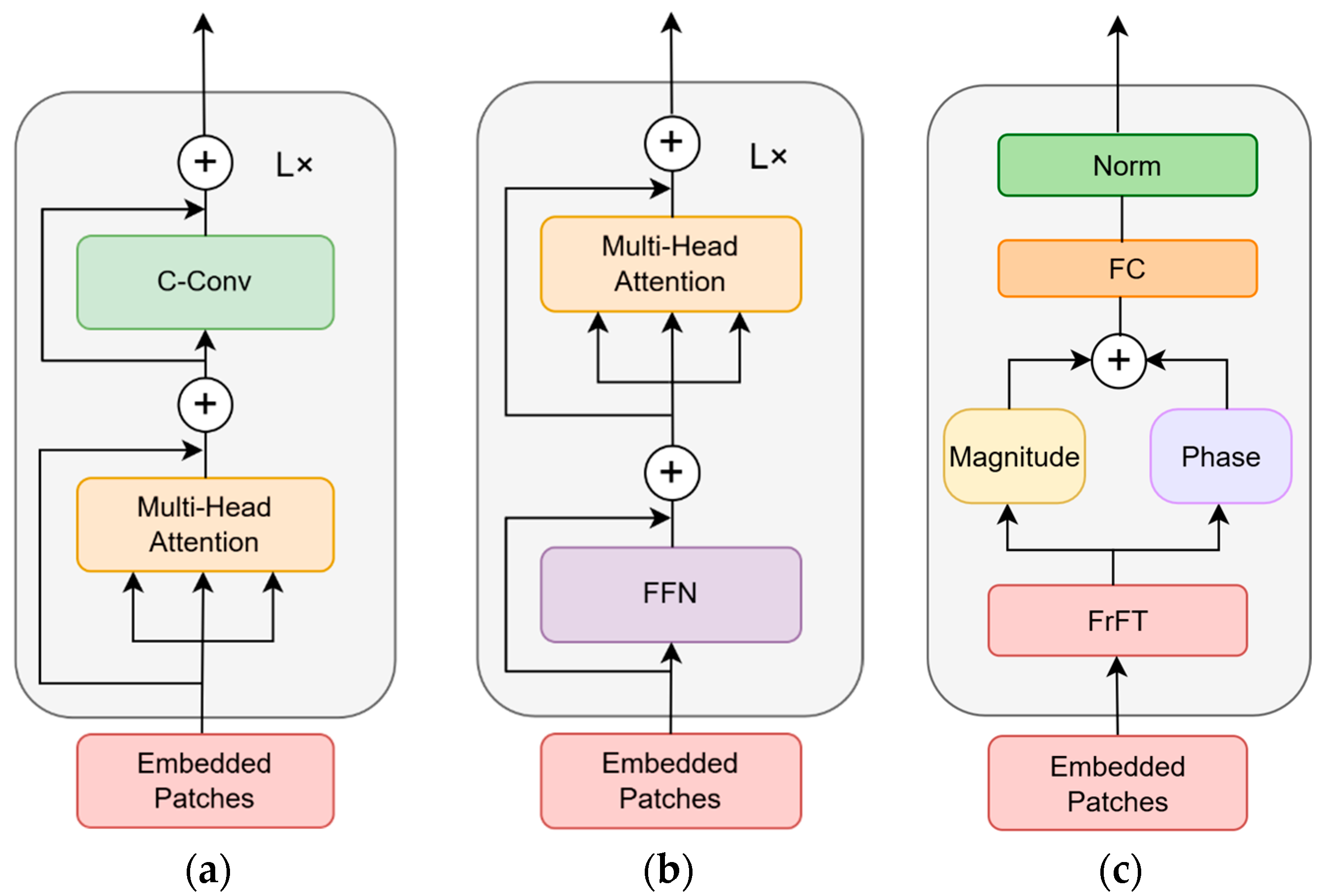
Based on the traditional ViT module, the three-branch parallel architecture is adopted by the FCViT model to realize multi-dimensional feature processing. The first branch adopts the dual design of “attention–convolution”; the second branch constructs the cascade structure of “feed-forward network–attention”; and the third branch innovatively introduces the FFT module for frequency domain analysis, which complements the spatial domain processing of the other two branches.

For forward propagation, the input tensor is fed synchronously into three branches: an attention–convolution branch that generates spatial features, a feed-forward–attention branch that generates structural features, and an FFT branch that produces spectral features. Finally, the three key pieces of information of spatial relationship, structural transformation, and frequency domain characteristics are organically integrated through the fusion strategy of element-by-element addition of three-way features. The multi-branch synergistic design enables a single Transformer module to simultaneously possess the three major capabilities of global attention modeling, local convolutional perception, and spectral analysis, which significantly enhances the richness of feature representation. The three-branch module branching diagram is shown in Figure 6.

In the “spatial–structural hybrid features” generated by the attention–convolution branch, the multi-head self-attention mechanism captures global dependencies, and then local features are extracted through the convolutional layer, and residual connections are used in both stages to maintain the original information. Convolutional operations mainly capture local spatial patterns through their local sensory field characteristics, while the front attention layer establishes global spatial relationships, and global context modeling can compensate for the local limitations of pure convolution to form a “local–global” synergistic spatial understanding. The attention–convolution branching diagram is shown in Figure 6a.

The feed-forward network–attention branch generates “structured semantic features”, which are first transformed by a two-layer MLP containing GELU activation, and then accessed by a second attention layer to form a more complex feature reorganization path. Cross-channel information fusion is used in implicit feature space by forcing the model through feature dimension transformations. On the basis of the FFN-transformed features, the secondary attention mechanism reconstructs the dynamic weight relationships among the tokens and performs context-aware filtering of the higher-order semantic features generated by the FFN. The feed-forward network–attention branching diagram is shown in Figure 6b.

FrFT frequency domain branching generates “frequency domain perceptual features”, the core value of which is to break through the limitations of the conventional Vision Transformer that only focuses on air domain features, and reveal the essential energy distribution and time–frequency characteristics of the signal through the frequency domain analysis, which is more robust to the operation of rotation and scaling. The FFN frequency domain branching diagram is shown in Figure 6c.

2.5. FCViT Model

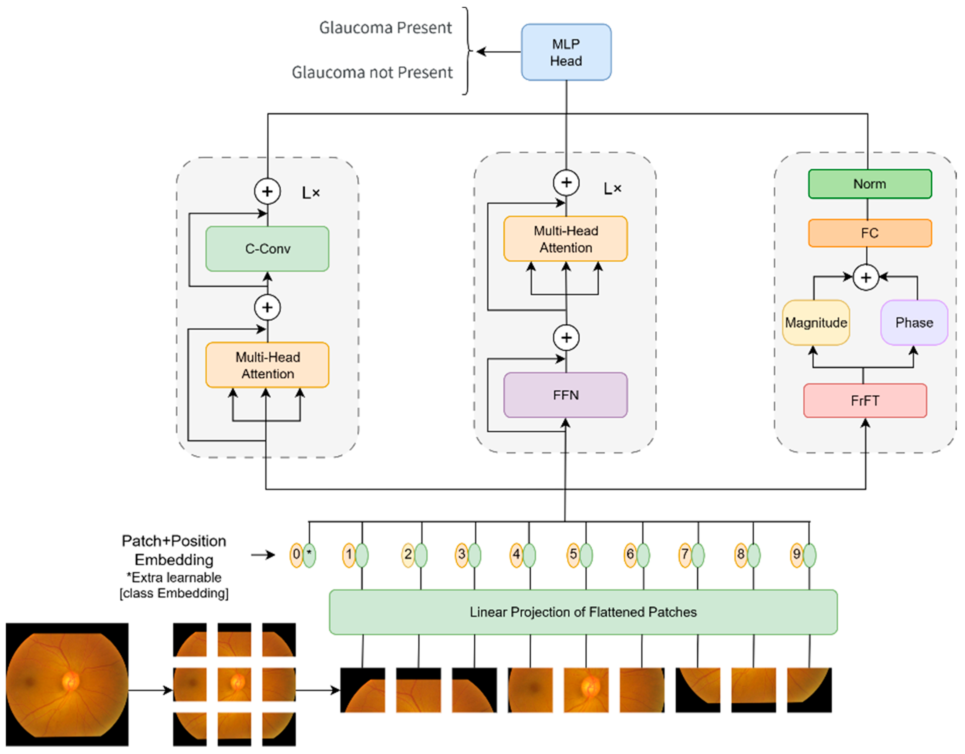
The three-branch feature extraction mechanism in the standard ViT architecture is innovatively introduced by the FCViT model to realize multi-dimensional feature fusion through the synergistic work of time domain convolution, frequency domain analysis, and an attention mechanism. The core component adopts residual connection design, in which the custom convolution module adopts dimensional rearrangement to realize channel-space dimension conversion, completes feature interaction while maintaining computational efficiency, and finally retains the original feature information through residual connection.

The frequency domain feature extraction branch obtains a more flexible frequency characterization capability by performing a hybrid time–frequency domain transform on the input sequence. The module utilizes trainable fractional-order parameters to control the depth of the transform, enabling the model to adaptively adjust its representation between the time and frequency domains to more accurately capture the structural features of the signal at different scales. After the fractional-order transformation, the extracted amplitude and phase features are compressed and stabilized by linear projection and layer normalization, which further enhances the model’s ability to recognize complex textures and non-smooth patterns, and improves the overall feature expression quality and discrimination performance.

Three branches construct a multipath feature learning system: the first branch uses the standard multi-head attention mechanism in series with the convolutional module; the second branch is connected in parallel with the attention mechanism via a two-layer MLP; and a new third branch handles frequency domain features. The outputs of the three branches are fused by simple summation to achieve feature fusion, which retains the global modeling capability of ViT and enhances the local feature extraction and frequency domain analysis. The FCViT network model diagram is shown in Figure 7.

3. Experimental Section

3.1. Common Experimental Models

The MobileNetV1 [24] model proposed by Google Research groundbreakingly redefined the design paradigm of efficient neural networks, and its core innovation is to decompose the standard convolution into more efficient computational units, laying the foundation for the subsequent development of deep learning models for mobile applications. Google Research followed with the MobileNetV2 [25] lightweight neural network architecture, which compresses the computation to less than 1/10th of the traditional CNN and has become a benchmark architecture for mobile deployment. MobileNetV3 [26], proposed by the Google Brain team, represents a landmark breakthrough in lightweight neural network design, and its innovations have significantly influenced the direction of deep learning in mobile applications.

The EfficientNet family of models proposed by the Google Brain team achieves an unprecedented balance between computational efficiency and model performance. The lightweight baseline model EfficientNet-B0 [27] has key features including the Mobile Inverted Bottleneck module and progressive resolution adjustment. The EfficientNetV2 [28] model is a comprehensive upgrade of the EfficientNet model, aiming to address the bottleneck of the original model in terms of training speed and parameter efficiency.

The ResNet model is a deep convolutional neural network architecture proposed by Kaiming He’s team, and its core innovation lies in the introduction of a residual learning mechanism, which effectively solves the problems of gradient vanishing and network degradation in deep network training. The ResNet model architecture not only sets a new performance benchmark for the field of computer vision, but has also become the basic design paradigm for all kinds of deep neural networks, which has a profound and lasting impact on the development of deep learning technology as a whole.

3.2. Datasets

The entire experimental code was written using the PyTorch framework. The programming language used was Python 3.11, with torch version 2.0.1, torchvision version 0.15.0, and wandb version 0.16.0.

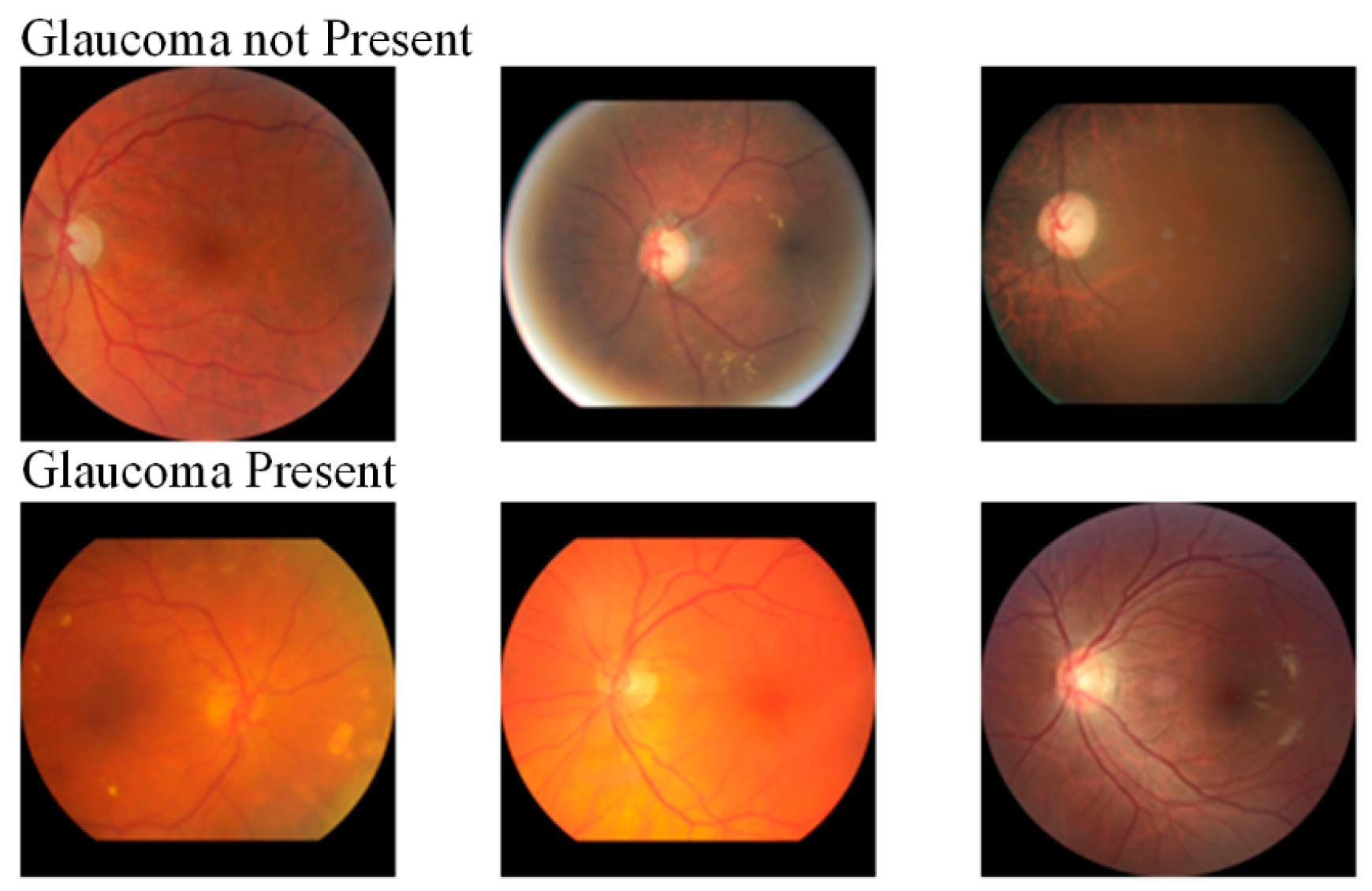
The retinal vasculature in fundus images shows a typical fractal structure with remarkable self-similarity and complex branching patterns, a structural feature that is particularly evident in the progression of glaucoma. Glaucoma is usually accompanied by optic nerve atrophy and changes in vascular morphology, leading to changes in fractal dimensions. Standardized fundus glaucoma dataset [29] images and the Harvard Dataverse-V1 [30] (HDV1) dataset were used for experimental evaluation in this paper. The standardized fundus glaucoma dataset includes two different categories: glaucoma present and glaucoma not present. The glaucoma present category accounted for 5293 samples and the glaucoma not present category accounted for 3328 samples, and the fundus images were in color. The HDV1 dataset includes three categories: early glaucoma, advanced glaucoma, and normal. The early glaucoma category accounted for 289 samples, the advanced glaucoma category accounted for 467 samples, and the normal category accounted for 786 samples. Since the experiments require a large amount of data for training, data augmentation experiments are performed on the HDV1 dataset for dataset expansion. The number of images in the standardized fundus glaucoma dataset and the HDV1 dataset is shown in

Table 1. Number of images in the standardized fundus glaucoma dataset and HDV1 dataset.

Dataset	Class Name	Total	Category
Standardized fundus blue light	Glaucoma Present	5293	2
	Glaucoma Not Present	3328
HDV1	Advanced Glaucoma	4670	3
	Early Glaucoma	2890
	Normal	3940

.

A randomly selected sample of images from the standard fundus glaucoma dataset is shown in Figure 8.

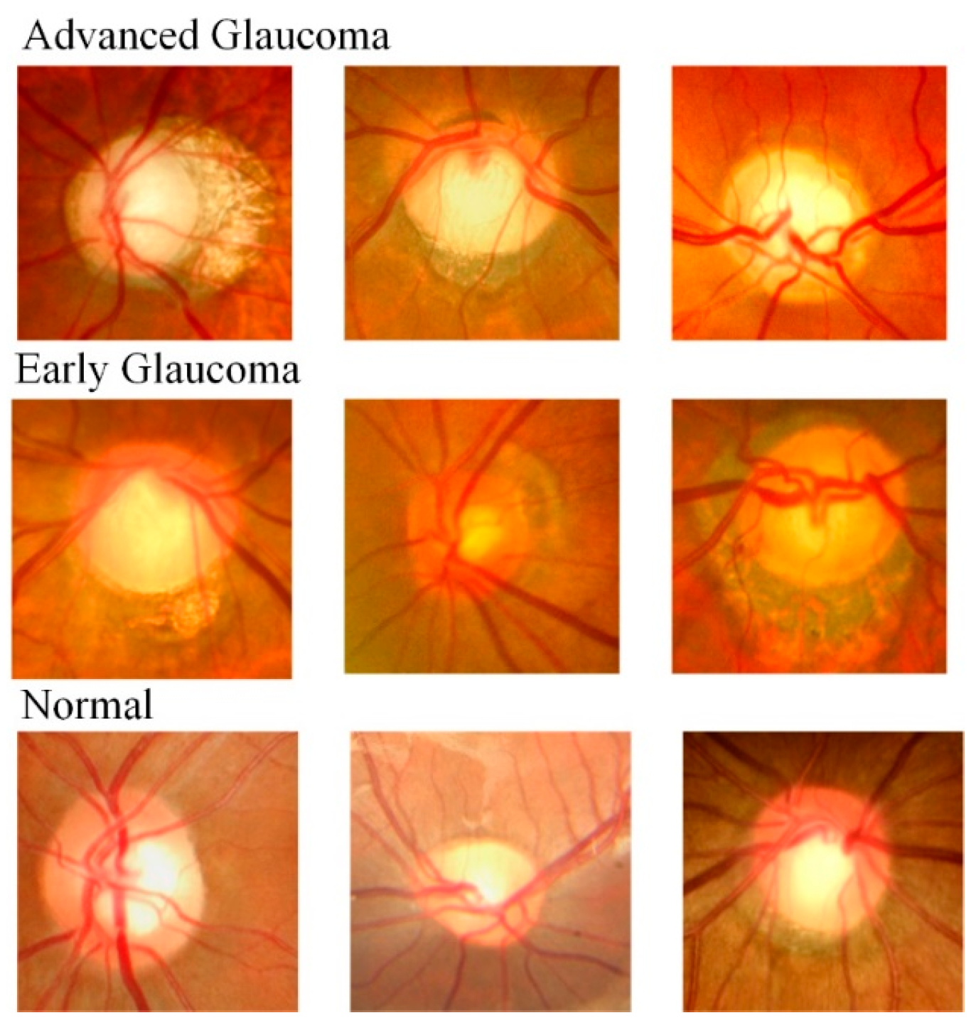
A randomly selected sample of images from the HDV1 dataset is shown in Figure 9.

3.3. Performance Indicator Test

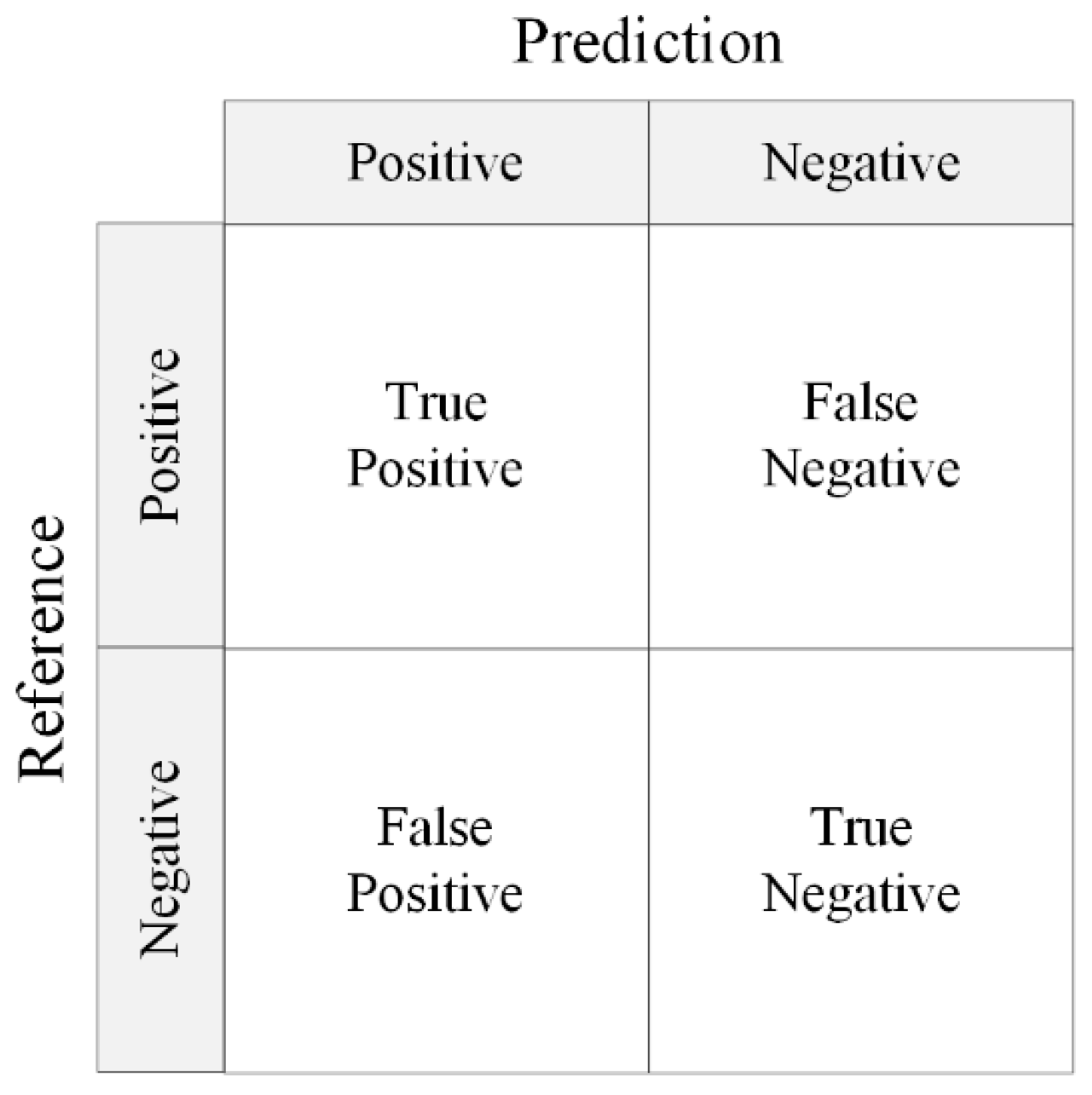
A confusion matrix is an important tool for evaluating the performance of classification models in machine learning, which visualizes the correspondence between the model predictions and the true labels in the form of a matrix. The rows of the matrix represent the true categories and the columns represent the predicted categories, revealing the model’s categorization preferences and error patterns by counting the distribution of samples across categories. The structure of the confusion matrix is shown in Figure 10.

The confusion matrix builds a cornerstone framework for model evaluation through four underlying quantitative metrics. True Positive (TP) reflects the model’s ability to correctly identify positive class samples and is a direct reflection of the model’s core efficacy; False Positive (FP) exposes the model’s over-sensitive tendency to misclassify negative classes as positive; False Negative (FN) reveals the model’s flawed under-detection of positive class samples; and True Negative (TN), on the other hand, demonstrates the model’s level of correct exclusion of negative class samples.

Accuracy measures the overall proportion of correct predictions made by the model for all samples, precision reflects the degree of confidence with which the model makes positive judgments, recall measures the model’s ability to capture positively classified samples, and F1-score is the reconciled average of precision and recall. The FCViT model was evaluated from different perspectives based on accuracy, precision, recall, and F1-score metrics. The accuracy, precision, recall, and F1-score are calculated as shown in Equations (20)–(23):

$$Accuracy={\displaystyle \frac{TP+TN}{TP+TN+FP+FN}}$$

(20)

$$Precision={\displaystyle \frac{TP}{TP+FP}}$$

(21)

$$Recall={\displaystyle \frac{TP}{TP+FN}}$$

(22)

$$F1-\mathrm{score}={\displaystyle \frac{2\times Precision\times Recall}{Precision+Recall}}$$

(23)

3.4. Experimental Results and Analysis

On the standardized fundus glaucoma dataset, the FCViT model achieved an accuracy of 93.52%, precision of 93.32%, recall of 92.79%, F1-score of 93.04%, and loss value of 0.249. Compared to the ViT_B_16 model the accuracy is improved by 6.21%, precision by 6.73%, recall by 6.27%, and F1-score by 6.75%. Compared with the MaxViT_T model, the accuracy, precision, recall, and F1-score are improved by 7.40%, 4.35%, 7.6%, and 8.46%, respectively; and compared with the SmallViT model, the accuracy, precision, recall, and F1-score are improved by 7.78%, 8.52%, 9.17%, and 9.83%. The FCViT model achieves better performance in terms of accuracy, precision, and F1-score compared to other commonly used traditional convolutional models. Early glaucoma symptoms are insidious and optic nerve damage is irreversible. A 1% improvement in accuracy may mean earlier detection of high-risk patients and avoidance of vision loss, while it may also reduce the amount of physician review and improve screening efficiency. The results of the model validation set for the standardized fundus glaucoma dataset are shown in

Table 2. Results of the model validation set for the standardized fundus glaucoma dataset.

Model	Accuracy (%)	Precision (%)	Recall (%)	F1-Score (%)	Loss
MobileV2	84.73	83.56	82.91	83.20	0.513
MobileV3_Small	85.25	84.01	84.58	83.71	0.525
MobileV3_Large	84.37	83.91	83.80	83.83	0.520
EfficientNet_B0	84.81	84.80	84.68	83.09	0.506
EfficientNet_B1	87.08	85.98	85.60	85.97	0.391
ResNet18	88.02	87.41	84.51	85.03	0.429
ResNet34	87.17	88.36	87.59	87.31	0.512
ResNet50	88.44	88.25	87.36	87.04	0.447
ShuffleNetV2	85.16	84.23	83.26	82.52	0.468
SqueezeNet	87.69	85.49	85.71	85.02	0.396
VGG11	85.40	86.40	86.16	86.28	0.451
VGG13	86.90	87.36	86.14	86.63	0.445
ViT_B_16	87.31	86.59	86.52	86.29	0.461
MaxViT_T	86.12	88.97	85.19	84.58	0.430
SmallViT	85.74	84.80	83.62	83.21	0.539
FCViT	93.52	93.32	92.79	93.04	0.249

.

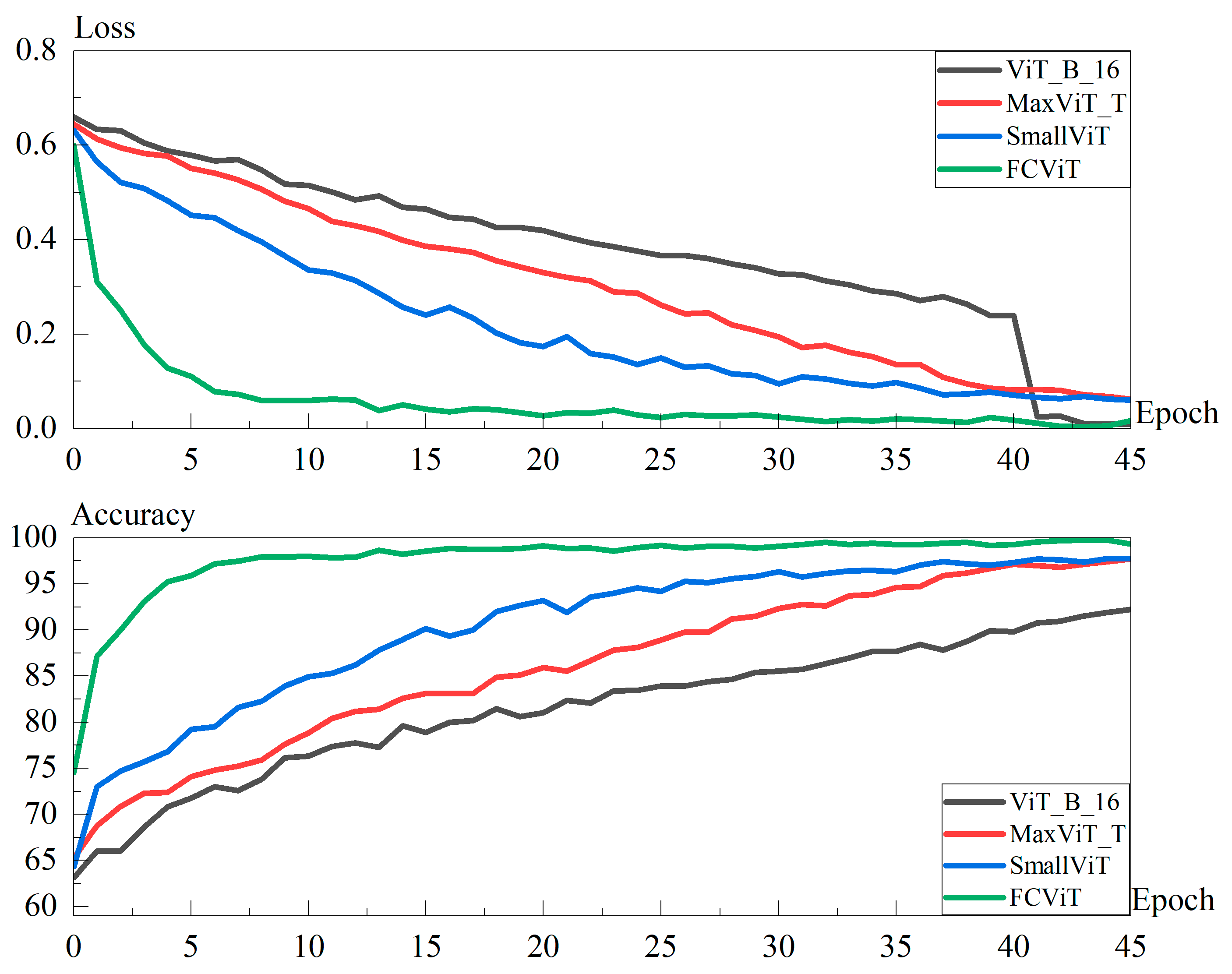
The results of the training set for the standardized fundus glaucoma dataset are shown in Figure 11.

Figure 11displays the number of iterations (45 rounds) on the standardized fundus glaucoma dataset where the FCViT model has saturated and is in a stable state for demonstration. The FCViT model saturates its performance around 20 rounds of iterations, showing significant and efficient convergence characteristics. In contrast, the comparison models, such as MaxViT_T, SmallViT, and ViT_B_16, are still in the stage of performance increase and have not yet reached a stable state. The experimental results fully demonstrate the advantages of the FCViT model in terms of training efficiency and convergence speed, and its well-designed hybrid architecture can learn effective feature representations faster.

The results of the standardized fundus glaucoma dataset model test set are shown in Figure 12.

As can be seen from Figure 12, the FCViT model shows excellent performance in all key evaluation metrics, and the accuracy, recall, and F1-score are significantly improved over mainstream models such as MaxViT_T and SmallViT. On the test set, the 95% confidence interval for the accuracy of the FCViT model is [92.86%, 95.13%]; the 95% confidence interval for F1-score is [92.43%, 94.81%].

The results of the model validation set for the HDV1 dataset are shown in

Table 3. Results of the model validation set for the HDV1 dataset.

Model	Accuracy (%)	Precision (%)	Recall (%)	F1-Score (%)	Loss
MobileV2	77.44	75.80	75.43	75.56	0.580
MobileV3_Small	78.78	77.30	76.98	77.11	1.208
MobileV3_Large	77.73	76.95	76.35	76.43	1.079
EfficientNet_B0	78.08	76.98	76.30	76.47	0.597
EfficientNet_B1	77.39	75.78	74.31	74.74	0.539
ResNet18	84.72	84.18	83.01	83.38	0.544
ResNet34	85.42	84.84	83.29	83.82	0.740
ResNet50	84.66	83.90	83.43	83.56	0.724
ConvNeXt	80.95	80.66	79.03	79.35	0.479
ShuffleNetV2	77.71	76.15	75.09	75.43	0.508
SqueezeNet	78.57	77.131	76.15	76.38	0.509
VGG11	85.21	84.94	83.48	83.96	0.476
VGG13	85.15	84.24	83.69	83.85	0.476
VGG16	84.34	83.14	82.71	82.89	0.514
ViT_B_16	91.04	90.26	90.26	90.24	0.380
MaxViT_T	90.66	89.69	89.80	89.70	0.317
SmallViT	85.18	84.24	83.59	83.73	0.634
FCViT	94.21	93.73	93.67	93.68	0.237

.

The FCViT model achieved better performance in terms of accuracy, precision, and F1-score compared to other commonly used models. The FCViT model achieved an accuracy of 94.86%, precision of 94.64%, recall of 94.30%, F1-score of 94.46%, and loss value of 0.237. Compared to the ViT_B_16 model the accuracy is improved by 3.17%, precision by 3.47%, recall by 3.41%, and F1-score by 3.44%; compared to the MaxViT_T model, its accuracy, precision, recall, and F1-score are improved by 3.55%, 4.04%, 3.87%, and 3.98%, respectively; compared to the SmallViT model its performance results are more significantly improved, with 9.03%, 9.49%, 10.08%, and 9.95% improvements in accuracy, precision, recall, and F1-score, respectively.

A comparison of the epoch time and number of parameters for the selected models in HDV1 is shown in

Table 4. Comparison of epoch time and number of parameters for selected models in HDV1.

	MaxViT_T	SmallViT	ViT_B_16	FCViT
Epoch Time	112.083	163.473	177.986	197.484
Parameter (M)	30.391	85.612	57.300	117.508

.

From the data in Table 4, it can be seen that in the case where the FCViT model has more parameters than the ViT_B_16 model, the time for iterating a single round is the same as the time for iterating a single round for the ViT_B_16 model.

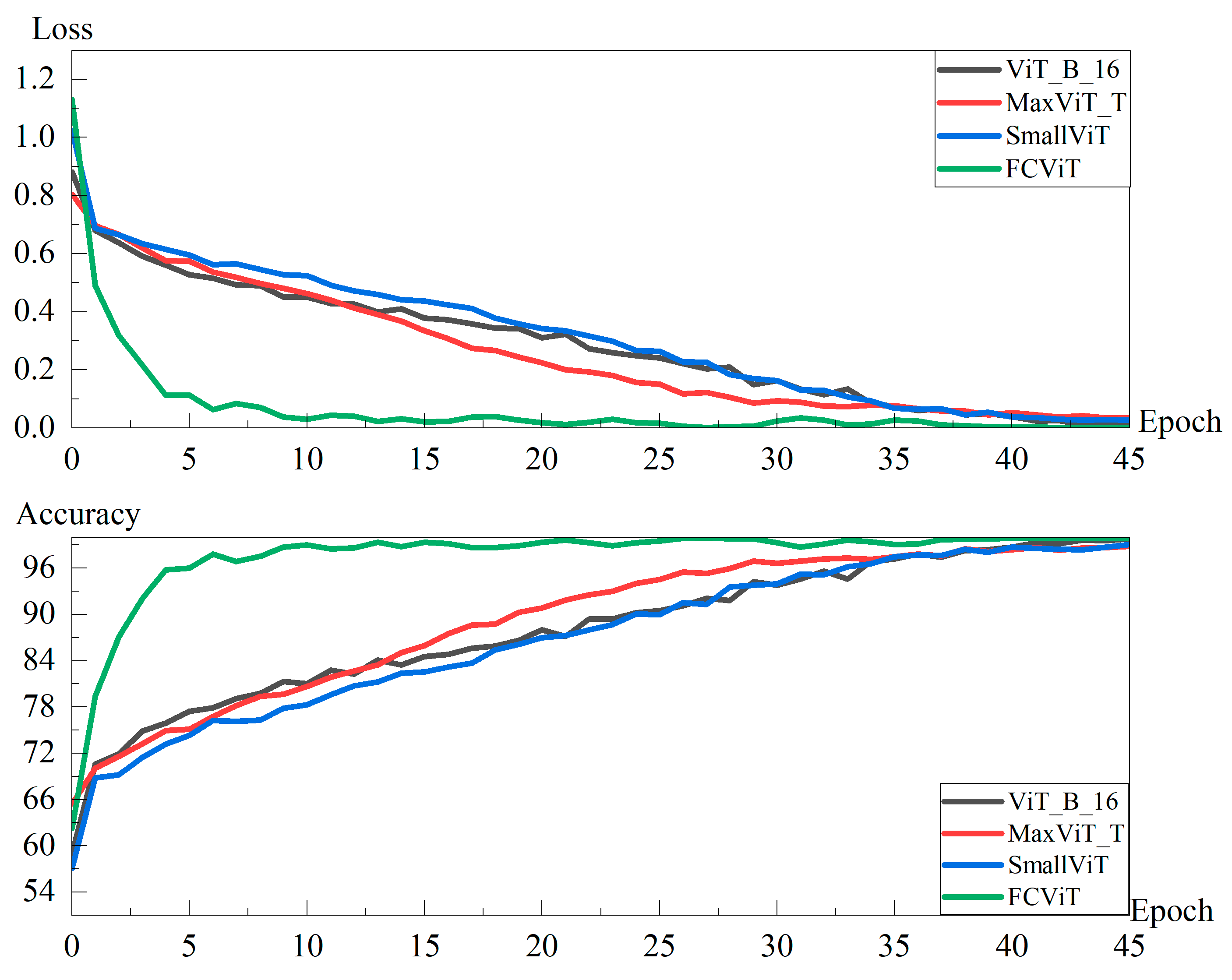
The results of the HDV1 dataset training set are shown in Figure 13.

As can be seen from Figure 13, the FCViT model saturates at around the tenth round, while the MaxViT_T model, SmallViT model, and ViT_B_16 model saturate at around 45 rounds of iterations. Compared to traditional models that often require dozens or even hundreds of iterations to stabilize, the FCViT model captures the essential laws of the data in a very short period of time, while its generalization robustness allows the model to converge quickly while maintaining excellent prediction reliability. The training curve shows that the model’s training set performance is always stabilized in the ideal interval after reaching the saturation point, indicating that its learning process is not disturbed by noise and has a strong resistance to overfitting.

The results of the HDV1 dataset test set are shown in Figure 14.

As can be seen from the experimental data in Figure 14, the FCViT model significantly outperforms MaxViT_T, SmallViT, and other comparative models in terms of core metrics such as accuracy, recall, and F1-score, demonstrating an all-round performance advantage. The FCViT model has good generalization capabilities across different tasks, ensuring robust performance. On the test set, the 95% confidence interval for the accuracy of the FCViT model is [91.30%, 94.17%]; the 95% confidence interval for the F1-score is [90.68%, 93.76%].

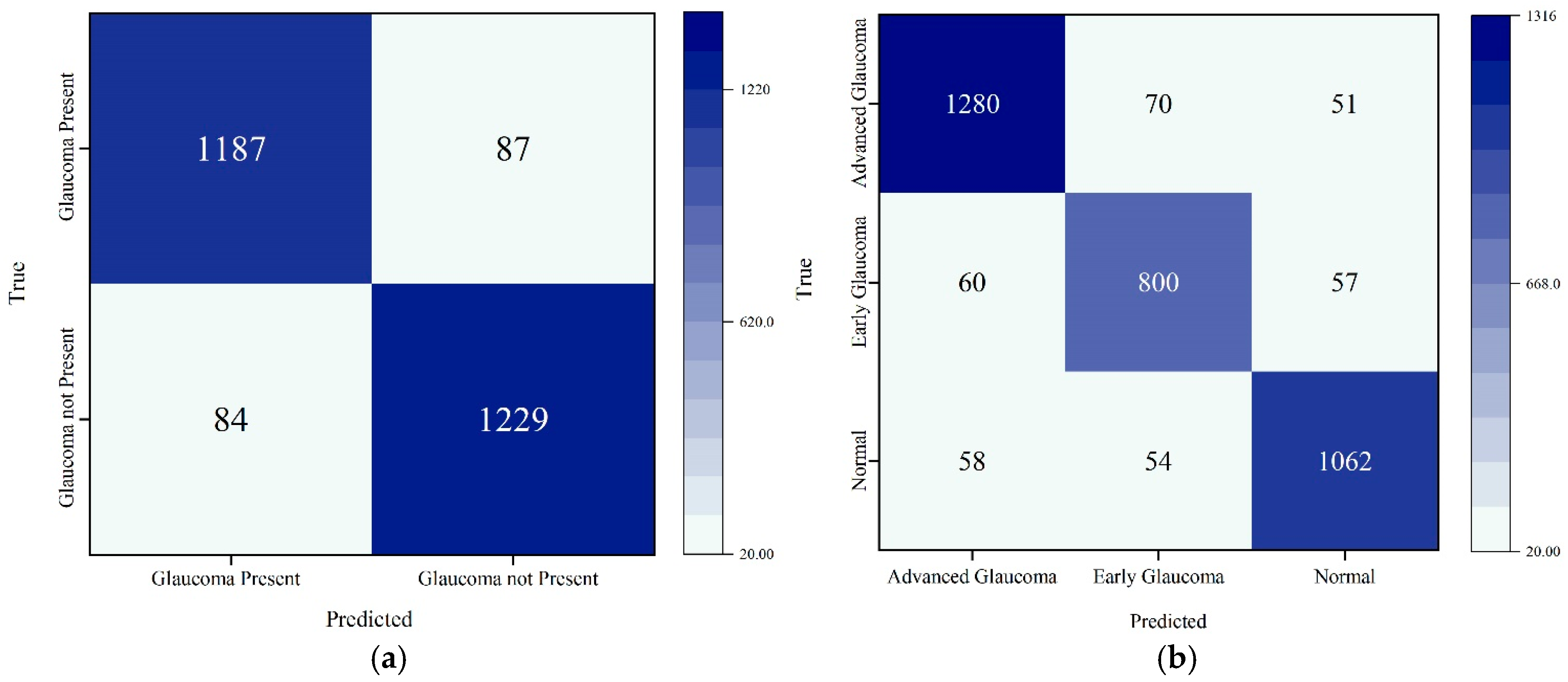
The FCViT model confusion matrix is shown in Figure 15.

In Figure 15a, the overall accuracy of the model is 93.69%, meaning it can correctly predict whether one has glaucoma in most cases. The model is able to accurately identify samples with glaucoma and can also help find most patients with glaucoma in practical applications. In Figure 15b, the model correctly classifies a high percentage of all samples. The model performs well overall, with the vast majority of samples being correctly classified. Late glaucoma was predicted most accurately in the model, and early glaucoma was also relatively accurate, reflecting to a large extent the ability of the model to recognize all stages of glaucoma, providing strong support in early screening and intervention.

4. Conclusions

Adopting a multi-branch parallel architecture, the Fourier Convolution Vision Transformer (FCViT) model, which combines the frequency domain analysis capability of Fractional-order Fourier Transform, the local feature extraction advantage of a convolution operation, and the global modeling capability of a self-attention mechanism, is proposed in this paper, realizing multi-level feature fusion, and demonstrating in the glaucoma classification task excellent performance. It performs particularly well on datasets from different sources, reaching 93.52%, 93.32%, 92.79%, and 93.04% for accuracy, precision, recall, and F1-score on the standardized fundus glaucoma dataset, respectively. The accuracy, precision, recall, and F1-score on the Harvard Dataverse-V1 dataset reached 94.21%, 93.73%, 93.67%, and 93.68%.

The FCViT model is able to capture both local details and global contextual information in medical images, accurately identifying key features of glaucoma as well as understanding a larger range of structural variations in complex images, thus significantly improving the classification performance and demonstrating stronger generalization ability under different data distributions. The FCViT model effectively avoids overfitting and captures the essential features of the complex disease of glaucoma, rather than relying solely on noise or specific biases that may be present in the data. In the context of medical image classification, the variability in the quality and diversity of datasets is frequently identified as a significant factor contributing to model overfitting. In contrast, the FCViT model’s capacity to consistently exhibit robust performance across diverse data sources is indicative of its superior adaptability and stability. This renders the FCViT model a promising candidate for real-time medical image analysis and diagnosis, offering a novel approach and technological solution for the early detection of glaucoma.

References

1. van Le, C. Unveiling Global Discourse Structures: Theoretical Analysis and NLP Applications in Argument Mining. arXiv 2025, arXiv:2502.08371. [Google Scholar] [CrossRef]
2. He, K.; Zhang, X.; Ren, S.; Sun, J. Deep residual learning for image recognition. In Proceedings of the IEEE Conference on Computer Vision and Pattern Recognition, Las Vegas, NV, USA, 27–30 June 2016; pp. 770–778. [Google Scholar]
3. Zaremba, W.; Sutskever, I.; Vinyals, O. Recurrent neural network regularization. arXiv 2014, arXiv:1409.2329. [Google Scholar]
4. Vaswani, A.; Shazeer, N.; Parmar, N.; Uszkoreit, J.; Jones, L.; Gomez, A.N.; Kaiser, Ł.; Polosukhin, I. Attention is all you need. Adv. Neural Inf. Process. Syst. 2017, 30, 6000–6010. [Google Scholar]
5. Guo, M.H.; Xu, T.X.; Liu, J.J.; Liu, Z.N.; Jiang, P.T.; Mu, T.J.; Zhang, S.H.; Martin, R.R.; Cheng, M.M.; Hu, S.M. Attention mechanisms in computer vision: A survey. Comp. Vis. Media 2022, 8, 331–368. [Google Scholar] [CrossRef]
6. Devlin, J.; Chang, M.W.; Lee, K.; Toutanova, K. Bert: Pre-training of deep bidirectional transformers for language understanding. In Proceedings of the 2019 Conference of the North American Chapter of the Association for Computational Linguistics: Human Language Technologies, Minneapolis, MN, USA, 2–7 June 2019; Volume 1, pp. 4171–4186. [Google Scholar]
7. Radford, A.; Narasimhan, K.; Salimans, T.; Sutskever, I. Improving Language Understanding by Generative Pre-Training. Available online: https://gwern.net/doc/www/s3-us-west-2.amazonaws.com/d73fdc5ffa8627bce44dcda2fc012da638ffb158.pdf (accessed on 28 March 2025).
8. Dosovitskiy, A.; Beyer, L.; Kolesnikov, A.; Weissenborn, D.; Zhai, X.; Unterthiner, T.; Dehghani, M.; Minderer, M.; Heigold, G.; Gelly, S.; et al. An Image is Worth 16x16 Words: Transformers for Image Recognition at Scale. arXiv 2021, arXiv:2010.11929. [Google Scholar] [CrossRef]
9. Liu, Z.; Lin, Y.; Cao, Y.; Hu, H.; Wei, Y.; Zhang, Z.; Lin, S.; Guo, B. Swin transformer: Hierarchical vision transformer using shifted windows. In Proceedings of the IEEE/CVF International Conference on Computer Vision, Montreal, BC, Canada, 11–17 October 2021; pp. 10012–10022. [Google Scholar]
10. Yang, J.; Li, C.; Zhang, P.; Dai, X.; Xiao, B.; Yuan, L.; Gao, J. Focal self-attention for local-global interactions in vision transformers. arXiv 2021, arXiv:2107.00641. [Google Scholar]
11. Hatamizadeh, A.; Nath, V.; Tang, Y.; Yang, D.; Roth, H.R.; Xu, D. Swin unetr: Swin transformers for semantic segmentation of brain tumors in MRI images. In International MICCAI Brainlesion Workshop; Springer: Cham, Switzerland, 2021; pp. 272–284. [Google Scholar]
12. Carion, N.; Massa, F.; Synnaeve, G.; Usunier, N.; Kirillov, A.; Zagoruyko, S. End-to-end object detection with transformers. In European Conference on Computer Vision; Springer: Cham, Switzerland, 2020; pp. 213–229. [Google Scholar]
13. Li, S.; Jin, X.; Xuan, Y.; Zhou, X.; Chen, W.; Wang, Y.X.; Yan, X. Enhancing the locality and breaking the memory bottleneck of transformer on time series forecasting. Adv. Neural Inf. Process. Syst. 2019, 32. [Google Scholar] [CrossRef]
14. Ying, C.; Cai, T.; Luo, S.; Zheng, S.; Ke, G.; He, D.; Shen, Y.; Liu, T.Y. Do transformers really perform badly for graph representation? Adv. Neural Inf. Process. Syst. 2021, 34, 28877–28888. [Google Scholar]
15. Strudel, R.; Garcia, R.; Laptev, I.; Schmid, C. Segmenter: Transformer for semantic segmentation. In Proceedings of the IEEE/CVF International Conference on Computer Vision, Montreal, BC, Canada, 11–17 October 2021; pp. 7262–7272. [Google Scholar]
16. He, K.; Chen, X.; Xie, S.; Li, Y.; Dollár, P.; Girshick, R. Masked autoencoders are scalable vision learners. In Proceedings of the IEEE/CVF Conference on Computer Vision and Pattern Recognition, New Orleans, LA, USA, 18–24 June 2022; pp. 16000–16009. [Google Scholar]
17. Bao, H.; Dong, L.; Piao, S.; Wei, F. BEiT: BERT Pre-Training of Image Transformers. arXiv 2022, arXiv:2106.08254. [Google Scholar] [CrossRef]
18. Fein-Ashley, J.; Feng, E.; Pham, M. HVT: A Comprehensive Vision Framework for Learning in Non-Euclidean Space. arXiv 2024, arXiv:2409.16897. [Google Scholar] [CrossRef]
19. Alotaibi, A.; Alafif, T.; Alkhilaiwi, F.; Alatawi, Y.; Althobaiti, H.; Alrefaei, A.; Hawsawi, Y.; Nguyen, T. ViT-DeiT: An ensemble model for breast cancer histopathological images classification. In Proceedings of the 1st International Conference on Advanced Innovations in Smart Cities (ICAISC), Jeddah, Saudi Arabia, 23–25 January 2023; pp. 1–6. [Google Scholar]
20. Krishnan, K.S.; Krishnan, K.S. Vision Transformer Based COVID-19 Detection Using Chest X-Rays. IEEE Conference Publication. In Proceedings of the 2021 6th International Conference on Signal Processing, Computing and Control (ISPCC), Solan, India, 7–9 October 2021; Available online: https://ieeexplore.ieee.org/document/9609375.
21. Wang, L.L.; Lo, K.; Chandrasekhar, Y.; Reas, R.; Yang, J.; Burdick, D.; Eide, D.; Funk, K.; Katsis, Y.; Kinney, R.; et al. CORD-19: The COVID-19 Open Research Dataset. arXiv 2024, arXiv:2004.10706. [Google Scholar] [CrossRef]
22. Wu, X.; Tao, R.; Hong, D.; Wang, Y. The FrFT convolutional face: Toward robust face recognition using the fractional Fourier transform and convolutional neural networks. Sci. China Inf. Sci. 2020, 63, 119103_1–119103_3. [Google Scholar] [CrossRef]
23. Barshan, B.; Ayrulu, B. Fractional Fourier transform pre-processing for neural networks and its application to object recognition. Neural Netw. 2002, 15, 131–140. [Google Scholar] [CrossRef] [PubMed]
24. Howard, A.G.; Zhu, M.; Chen, B.; Kalenichenko, D.; Wang, W.; Weyand, T.; Andreetto, M.; Adam, H. Mobilenets: Efficient convolutional neural networks for mobile vision applications. arXiv 2017, arXiv:1704.04861. [Google Scholar] [CrossRef]
25. Sandler, M.; Howard, A.; Zhu, M.; Zhmoginov, A.; Chen, L.C. Mobilenetv2: Inverted residuals and linear bottlenecks. In Proceedings of the IEEE Conference on Computer Vision and Pattern Recognition, Salt Lake City, UT, USA, 18–23 June 2018; pp. 4510–4520. [Google Scholar]
26. Howard, A.; Sandler, M.; Chu, G.; Chen, L.C.; Chen, B.; Tan, M.; Wang, W.; Zhu, Y.; Pang, R.; Vasudevan, V.; et al. Searching for mobilenetv3. In Proceedings of the IEEE/CVF International Conference on Computer Vision, Seoul, Republic of Korea, 27 October–2 November 2019; pp. 1314–1324. [Google Scholar]
27. Tan, M.; Le, Q. Efficientnet: Rethinking model scaling for convolutional neural networks. In Proceedings of the International Conference on Machine Learning, PMLR, Long Beach, CA, USA, 9–15 June 2019; pp. 6105–6114. [Google Scholar]
28. Tan, M.; Le, Q. Efficientnetv2: Smaller models and faster training. In Proceedings of the International Conference on Machine Learning, PMLR, Online, 18–24 July 2021; pp. 10096–10106. [Google Scholar]
29. Kiefer, R.; Abid, M.; Steen, J.; Ardali, M.R.; Amjadian, E. A Catalog of Public Glaucoma Datasets for Machine Learning Applications: A detailed description and analysis of public glaucoma datasets available to machine learning engineers tackling glaucoma-related problems using retinal fundus images and OCT images. In Proceedings of the 7th International Conference on Information System and Data Mining (ICISDM), Atlanta, GA, USA, 10–12 May 2023; pp. 24–31. [Google Scholar] [CrossRef]
30. Acharya, U.R.; Ng, E.Y.K.; Eugene, L.W.J.; Noronha, K.P.; Min, L.C.; Nayak, K.P.; Bhandary, S.V. Decision support system for the glaucoma using Gabor transformation. Biomed. Signal Process. Control 2015, 15, 18–26. [Google Scholar] [CrossRef]
Figure 1. Vision Transformer model architecture.
Fractalfract 09 00533 g001
Figure 2. Graphical representation of FFT operations.
Fractalfract 09 00533 g002
Figure 3. FrFT module.
Fractalfract 09 00533 g003
Figure 4. Customization of the Conv module layer.
Fractalfract 09 00533 g004
Figure 5. C-Conv module.
Fractalfract 09 00533 g005
Figure 6. Three-branch module branching diagram: (a) attention–convolution branching diagram; (b) feed-forward network–attention branching diagram; (c) FrFT frequency domain branching diagram.
Fractalfract 09 00533 g006
Figure 7. FCViT network module diagram.
Fractalfract 09 00533 g007
Figure 8. Randomly selected image samples from the standard fundus glaucoma dataset.
Fractalfract 09 00533 g008
Figure 9. Randomly selected sample of images from the HDV1 dataset.
Fractalfract 09 00533 g009
Figure 10. Confusion matrix structure.
Fractalfract 09 00533 g010
Figure 11. Results of the training set for the standardized fundus glaucoma dataset.
Fractalfract 09 00533 g011
Figure 12. Results of the standardized fundus glaucoma dataset model test set.
Fractalfract 09 00533 g012
Figure 13. Results of the HDV1 dataset training set.
Fractalfract 09 00533 g013
Figure 14. Results of the HDV1 dataset test set.
Fractalfract 09 00533 g014
Figure 15. FCViT model confusion matrix: (a) standardized fundus glaucoma dataset; (b) HDV1 dataset.
Fractalfract 09 00533 g015