Stability and Convergence Analysis of Compact Finite Difference Method for High-Dimensional Time-Fractional Diffusion Equations with High-Order Accuracy in Time

Abstract

Based on the spatial compact finite difference (SCFD) method, an improved high-order temporal accuracy scheme for high-dimensional time-fractional diffusion equations (TFDEs) is presented in this work. Combining the temporal piecewise quadratic interpolation and the high-dimensional SCFD method, the proposed numerical method is described. In order to establish the stability and convergence analysis, we introduce a norm $\left|\right|·{\left|\right|}_{{\tilde{H}}^1}$, which is rigorously proved equivalent to the standard $H^1$-norm. Considering that the coefficients of high-order numerical schemes are not entirely positive, we introduce an appropriate parameter to transform the numerical scheme into an equivalent form with positive coefficients. Based on the equivalent form, we prove that the temporal and spatial convergence orders are $(3-\gamma )$ and 4 by applying the convergence of geometric progression. The proposed scheme ensures that the theoretical convergence accuracy at each time step is of order $(3-\gamma )$ without requiring any additional processing techniques. Ultimately, the convergence of the proposed high-order accurate scheme is verified through numerical experiments involving (non-)linear high-dimensional TFDEs.

1. Introduction

The stability and convergence analysis of the high-order accurate numerical method for high-dimensional time-fractional diffusion equations (TFDEs), presented in this paper, holds significant intrinsic value and provides a crucial foundation for solving numerous other high-dimensional fractional partial differential equations (PDEs). The model equation controls the evolution of the probability density function that describes the anomalous diffusing particles. Anomalous diffusion deviates from the Fisher standard description of Brownian, whose main characteristic is a nonlinear increase of the mean squared displacement with respect to time, such as $<x^2(t)>\sim t^{\gamma }$. The TFDE describes the anomalous sub-diffusion corresponding to $0<\gamma <1$. Examples of sub-diffusive transport include turbulence and disordered dynamical carrier transport in amorphous semiconductors [1], NMR diffusometry in disordered materials [2], etc.

In recent years, fractional calculus has been widely applied to solve numerous scientific and engineering problems, including those in electromagnetics, physical sciences, diffusion, electrochemistry, and general transport theory. Many complex scientific and engineering problems are described more accurately and realistically by fractional-order PDEs than by integer-order PDEs, such as the synchronization of fractional order stochastic systems in finite-dimensional space [3], fractional-order learning [4], and the dynamic behavior of the hepatitis B-virus by the Caputo–Fabrizio fractional derivative [5] with the definition ${\displaystyle {}_0{}^{\mathit{CF}}D_t^{\gamma }u(t)=\frac{1}{1-\gamma }{\int }_0^t{u}^{\prime }(s)e^{-\frac{\gamma }{1-\gamma }(t-s)ds}}$. Many effective schemes have been developed to solve linear and nonlinear TFDEs, such as the spectral method [6], shifted Grünwald difference operator [7], Gaussian radial basis functions method [8], the L1-type scheme [9,10,11,12,13], the L2-type scheme [14,15], etc.

We are interested in the following high-dimensional TFDEs:

$$\left\{\begin{array}{c}{}_{0}D_t^{\gamma }u(\mathbf{x},t)-\sum _{i=1}^d{K}_i{\mathsf{\partial }}_{x_i}^{2}u(\mathbf{x},t)=f(\mathbf{x},t),\mathbf{x}\in \mathsf{\Omega },t\in (0,T],\hfill \\ u(\mathbf{x},t)=0,\mathbf{x}\in \mathsf{\partial }\mathsf{\Omega },t\in (0,T],\hfill \\ u(\mathbf{x},0)=u_0(\mathbf{x}),\mathbf{x}\in \mathsf{\Omega },\hfill \end{array}\right.$$

(1)

where $\mathbf{x}=(x_1,x_2,\cdots ,x_d)\in {\Re }^d$ with $d\ge 2$ is the dimension of the space. ${\displaystyle \mathsf{\Omega }=\prod _{i=1}^d(a_i,b_i)}$ $\subset {\Re }^d$ is bounded, T is a bounded positive constant, the boundary of $\mathsf{\Omega }$ is $\mathsf{\partial }\mathsf{\Omega }$, and $\overline{\mathsf{\Omega }}$ denotes the closure of $\mathsf{\Omega }$. The $\gamma$$(0<\gamma <1)$ order Caputo fractional derivative ${}_{0}D_t^{\gamma }$ [16] is defined as follows:

$$\begin{array}{c}\hfill {}_{0}D_t^{\gamma }u(\mathbf{x},t)={\displaystyle \frac{1}{\mathsf{\Gamma }(1-\gamma )}}{\int }_0^t{(t-s)}^{-\gamma }{\displaystyle \frac{\mathsf{\partial }u(\mathbf{x},s)}{\mathsf{\partial }s}}ds.\end{array}$$

Additionally, the Euler gamma function is represented as $\mathsf{\Gamma }(·)$, the diffusion constants are expressed as $K_i>0,i=1,2,\cdots ,d$, and the known smooth functions are represented as $u_0(\mathbf{x})$, $f(\mathbf{x},t)$. For clarity, in the following numerical analysis, we assume that Equation (1) has a unique and sufficiently smooth solution.

Considering the non-locality of fractional derivatives, the computational complexity of the numerical schemes for fractional derivatives is generally enormous. Therefore, constructing high-precision numerical schemes for fractional derivatives is a common approach to solving TFDEs. Due to the high-precision convergence of compact difference schemes (CFDs), such schemes are widely applicable in solving TFDEs by combining high-order temporal numerical methods. In [17], a fourth-order compact ADI scheme was constructed to solve a two-dimensional, time-fractional, reaction-subdiffusion equation. In [18], an efficient numerical scheme for the distributed order TFDE was developed by using the temporal L1 formula. In [19], a variable-step second-order weighted ADI scheme was used to solve the 2D time-fractional telegraph equation. In [20], two fast solvers were developed using time-marching and divide-and-conquer techniques. In [21], an L2-type temporal scheme was used, but with a low-order accuracy at the first time level, to solve the TFDE. In [22], a spatial sixth-order scheme was implemented to solve the TFDE with a temporal Caputo–Fabrizio fractional derivative. In [23], a fast high-order scheme for a fractal mobile/immobile transport model was presented with an FFT and a CFD scheme. In [24], a fourth-order compact ADI scheme was developed by applying the Padé approximation. In [25], a high-order two-grid scheme for nonlinear PDEs was proposed, and the high-order mapping operator method was employed. In [26], a CFD scheme was constructed to solve a time-fractional, fourth-order, integro-differential equation. In [27], a high-order CFD method was proposed to solve linear time-fractional subdiffusion equations using an L2-type scheme. In [28], a semilinear fractional initial-boundary value problem was solved and investigated using an L2-type time scheme.

However, the numerical schemes mentioned above are uniform temporal schemes designed for TFDEs with a smooth solution. In [29], the L1 method on a graded mesh was applied to solve the multi-term TFDEs with weak singularity by using a weak Galerkin finite element method in space. In [30], the authors introduced fast preconditioned iterative solvers for an all-at-once linear system based on Volterra sub-diffusion equations, employing a graded-step L1 scheme in time. In [31], a robust ADI scheme on a graded mesh was proposed for solving sub-diffusion problems in 3D using an L1-type scheme in time. In [32], a fast modified $\overline{L1}$ scheme was used to address the initial weakly singular solution of the TFDE. In [33], the initial singularity solution of the 2D time-fractional mobile/immobile diffusion problem was solved using the average L1-type scheme. In [34], a numerical scheme with nonuniform time steps for distributed order sub-diffusion equations related to the initial weakly singular solution was presented in the form of an L1-type scheme.

Several shortcomings exist in the current L2-type scheme. The existing numerical schemes can be divided into two main categories. The first type approximates the first time level using a low-order numerical scheme, which can disrupt the consistent convergence order of time in theoretical analysis. The second type focuses on exact solutions when the equation has a special form, such as when the right-hand term does not contain unknown variables, which cannot be applied to semi-nonlinear problems. In addition, the exiting CFD schemes for 2D and 3D TFDEs mainly use ADI schemes, which reduce time accuracy to improve computational efficiency. The idea of constructing the above scheme is not applicable to constructing a high-precision numerical scheme for high-dimensional TFDEs. Therefore, in this work, we construct an improved high-order uniform temporal accuracy scheme using a coupled numerical scheme in the first and second layers to enhance the convergence accuracy and avoid restrictions on the right-hand term. The first advantage of the numerical scheme of this article can be applied directly to solving nonlinear problems, as it benefits from its form without relying on the right-hand function. The second advantage is that the computational complexity of the numerical scheme presented in this paper is lower than that of existing numerical schemes when the accuracy of solving the problem is determined. According to the emerging literature, there are few studies on the SFCD scheme for 3D TFDEs. Therefore, this article provides a detailed convergence and stability analysis of the CFD scheme for high-dimensional TFDEs with high uniform temporal accuracy.

This paper is a continuation of the research in [35], in which detailed stability and convergence analysis are provided for a one-dimensional TFDE. In this paper, we provide a systematic theoretical analysis of the high-order numerical scheme for d-dimensional TFDEs ($d\ge 2$). The main strategies and innovations of this paper are as follows:

• A high-order accurate implicit difference scheme for high-dimensional TFDEs is developed by combining a spatial fourth-order CFD schemes with an improved temporal L2 scheme.
• The convergence of the improved numerical scheme for solving Equation (1) is established by introducing an appropriate parameter transformation to rewrite an equivalent form and using the convergence of the geometric progression.
• The improved numerical scheme ensures that the theoretical convergence accuracy at every time step is $(3-\gamma )$ without requiring additional processing techniques. This numerical scheme can be easily extended to solve semi-linear TFDEs like the time-fractional Allen–Cahn equation.
• The equivalence proof of the norm $\left|\right|·{\left|\right|}_{{\tilde{H}}^1}$ in the d-dimension and the standard $H^1$-norm is rigorously established, which is convenient for analyzing the stability and convergence analysis of the proposed method applied to d-dimensional TFDEs.

The remainder of this article is organized as follows. In Section 2, we present an improved high-order temporal accuracy scheme that incorporates the SCFD scheme for high-dimensional TFDEs. In Section 3, we provide detailed proofs for the stability and convergence analysis of the improved fully discrete scheme with spatial and temporal high-order accuracy. Some numerical results of the improved scheme are presented to solve TFDEs with smooth and non-smooth solutions in Section 4. In Section 5, we provide a short summary.

2. An Improved Fully Discrete High-Order Uniform Temporal Accuracy Scheme

In this section, we construct a high-order temporal accuracy scheme with the SCFD approximation and perform a theoretical analysis of high-dimensional TFDEs (1). For convenience, we refer mainly to the symbol representation in [36]. Assume that $N_i,i=1,2,\cdots ,d$ and K are $d+1$ positive integers and that the spatial grid size and temporal step-size are set as $\Delta x_i=(b_i-a_i)/N_i,\tau =T/K$. The spatial and temporal discrete points are defined as $x_{i,l}=a_i+l\Delta x_i(0\le l\le N_i,1\le i\le d)$, $t_n=n\tau (0\le n\le K)$.

For $1\le i\le d$, we define ${\mathsf{\Theta }}_i=\{l\in {\mathbb{N}}^{+}|1\le l\le N_i-1\}$ and ${\displaystyle {\ddot{\mathsf{\Theta }}}_i=\{l\in {\mathbb{N}}^{+}|0\le l\le N_i\},\mathsf{\Psi }=\prod _{i=1}^d{\mathsf{\Theta }}_i,\ddot{\mathsf{\Psi }}=\prod _{i=1}^d{\ddot{\mathsf{\Theta }}}_i}$ and $\mathsf{\partial }\ddot{\mathsf{\Psi }}=\ddot{\mathsf{\Psi }}\setminus \mathsf{\Psi }$. For simplicity, we set a multi-index $\mathbf{L}=(l_1,l_2,\cdots ,l_d)$ and denote ${\mathbf{x}}_{\mathbf{L}}=(x_{1,l_1},x_{2,l_2},\cdots ,x_{d,l_d})$, grid function $u_{\mathbf{L}}^n$, and exact function $u_{\mathbf{L}}^n=u({\mathbf{x}}_{\mathbf{L}},t_n)$ by $\mathbf{L}\in \ddot{\mathsf{\Psi }}$ and $0\le n\le K,f_{\mathbf{L}}^n=f({\mathbf{x}}_{\mathbf{L}},t_n)$.

Based on the idea of the definition in [37], we define the compact difference operators $H_i{u}_{\mathbf{L}}$ in the $x_i$$(i=1,2,\cdots ,d)$ directions, defined as follows:

$$\begin{array}{c}\hfill H_i{u}_{\mathbf{L}}=\left\{\begin{array}{cc}{\displaystyle (I+\frac{\Delta x_i^2}{12}{\delta }_{x_i}^2)u_{\mathbf{L}},}\hfill & 1\le i\le d,\mathbf{L}\in \mathsf{\Psi },\hfill \\ u_{\mathbf{L}},\hfill & \mathbf{L}\in \mathsf{\partial }\ddot{\mathsf{\Psi }},\hfill \end{array}\right.\end{array}$$

where I is the identical operator.

The discrete $H^1$ semi-norm and $H^1$ norm in d-dimensional space of the grid function u are given as

$$\begin{array}{c}\hfill \left|\right|{\nabla }_{h}u\left|\right|=\sqrt{\sum _{i=1}^d\left|\right|{\delta }_{x_i}u{\left|\right|}^2}{,\left|\right|u\left|\right|}_{H^1}={\sqrt{{\left|\right|u\left|\right|}^2+\left|\right|{\nabla }_{h}u\left|\right|}}^2.\end{array}$$

In this paper, instead of using the above standard $H^1$ norm, we prefer to define the inner products and ${\tilde{H}}^1$ norm as follows:

$$\begin{array}{c}\hfill {(u,v)}_{{\tilde{H}}^1}=\sum _{i=1}^d{K}_i{(\prod _{m=1,m\ne i}^d{H}_{m}u,\prod _{m=1,m\ne i}^d{H}_{m}v)}_{x_i}{,\left|\right|u\left|\right|}_{{\tilde{H}}^1}=\sqrt{\sum _{i=1}^d{K}_i\left|\right|\prod _{m=1,m\ne i}^d{H}_{m}u{\left|\right|}_{x_i}^2},\end{array}$$

(2)

where ${\left|\right|u\left|\right|}_{x_i}=\sqrt{{\displaystyle \left|\right|{\delta }_{x_i}{u\left|\right|}^2-\frac{\Delta {x_i}^2}{12}\left|\right|{\delta }_{x_i}^{2}u{\left|\right|}^2}},i=1,2,\cdots ,d$. It is easy to prove that ${(u,v)}_{x_i}$, ${(u,v)}_{{\tilde{H}}^1}$ are all inner products, and the corresponding norms as defined above.

Next, we prove that the $\left|\right|·{\left|\right|}_{{\tilde{H}}^1}$ norm in the d-dimension is equivalent to the standard $H^1$ norm, which is convenient for analyzing stability and convergence analysis. The author remarked that this proof is different from [37] (Lemma 3.2). Consider that the proof in [37] can only be generalized to the d-dimensional case when $d\le 3$. Therefore, this article provides a different proof for the d-dimensional case with $d\ge 2$ in the following Lemma 1.

Lemma 1.

For any grid function $u\in u_{\mathbf{L}}^n$, the following inequality holds:

$$\begin{array}{c}\hfill \sqrt{{\displaystyle {(\frac{2}{3})}^{2d-1}\underset{i}{min}\left\{K_i\right\}{\left(1+\frac{1}{C_{\mathsf{\Omega }}}\right)}^{-1}}}{\left|\right|u\left|\right|}_{H^1}\le {\left|\right|u\left|\right|}_{{\tilde{H}}^1}\le {({\displaystyle \frac{4}{3}})}^{d-1}\sqrt{\underset{i}{max}\left\{K_i\right\}}{\left|\right|u\left|\right|}_{H^1},\end{array}$$

where ${\displaystyle C_{\mathsf{\Omega }}=6\sum _{i=1}^d{(b_i-a_i)}^{-2}}$.

Proof. 

Using the inverse estimate $\left|\right|{\delta }_{x_i}^{2}u\left|\right|\le {\displaystyle \frac{2}{\Delta x_i}}\left|\right|{\delta }_{x_i}u\left|\right|\le {\displaystyle \frac{4}{\Delta x_i^2}}\left|\right|u\left|\right|,i=1,2,\cdots ,d$, we have

$$\begin{array}{c}\hfill \parallel H_{m}u\parallel =\parallel (I+{\displaystyle \frac{\Delta x_m^2}{12}}{\delta }_{x_m}^2)u\parallel \le \parallel u\parallel +{\displaystyle \frac{\Delta x_m^2}{12}}\parallel {\delta }_{x_m}^{2}u\parallel \le {\displaystyle \frac{4}{3}}\parallel u\parallel .\end{array}$$

(3)

In addition, we get

$$\begin{array}{c}\hfill \parallel H_{m}u\parallel \ge \parallel u\parallel -{\displaystyle \frac{\Delta x_m^2}{12}}\parallel {\delta }_{x_m}^{2}u\parallel \ge \parallel u\parallel -{\displaystyle \frac{\Delta x_m^2}{12}}·{\displaystyle \frac{2}{\Delta x_m}}·{\displaystyle \frac{2}{\Delta x_m}}\parallel u\parallel ={\displaystyle \frac{2}{3}}\parallel u\parallel .\end{array}$$

(4)

Combining (3) and (4), we obtain

$$\begin{array}{c}\hfill {\displaystyle \frac{2}{3}}\parallel u\parallel \le \parallel H_{m}u\parallel \le {\displaystyle \frac{4}{3}}\parallel u\parallel .\end{array}$$

(5)

Repeated the idea of inequality (5) gives the following inequality:

$$\begin{array}{c}\hfill {({\displaystyle \frac{2}{3}})}^{d-1}\parallel {\delta }_{x_i}u\parallel \le \parallel \prod _{m=1,m\ne i}^d{H}_m{\delta }_{x_i}u\parallel \le {({\displaystyle \frac{4}{3}})}^{d-1}\parallel {\delta }_{x_i}u\parallel .\end{array}$$

(6)

Next, we estimate ${\left|\right|u\left|\right|}_{{\tilde{H}}^1}$. More precisely,

$$\begin{array}{ccc}\hfill {\left|\right|u\left|\right|}_{{\tilde{H}}^1}^2& =& \sum _{i=1}^d{K}_i(\parallel \prod _{m=1,m\ne i}^d{H}_m{\delta }_{x_i}{u\parallel }^2-{\displaystyle \frac{\Delta x_i^2}{12}}\parallel \prod _{m=1,m\ne i}^d{H}_m{\delta }_{x_i}^{2}u{\parallel }^2)\hfill \\ & \le & \sum _{i=1}^d{K}_i\parallel \prod _{m=1,m\ne i}^d{H}_m{\delta }_{x_i}{u\parallel }^2\le \underset{i}{max}\left\{K_i\right\}\sum _{i=1}^d\parallel \prod _{m=1,m\ne i}^d{H}_m{\delta }_{x_i}{u\parallel }^2.\hfill \end{array}$$

Using the right-hand side of (6), we have

$$\begin{array}{c}\hfill {\left|\right|u\left|\right|}_{{\tilde{H}}^1}^2\le \underset{i}{max}\left\{K_i\right\}\sum _{i=1}^d{({\displaystyle \frac{4}{3}})}^{2d-2}\parallel {\delta }_{x_i}{u\parallel }^2={({\displaystyle \frac{4}{3}})}^{2d-2}\underset{i}{max}\left\{K_i\right\}\left|\right|{\nabla }_{h}u{\left|\right|}^2.\end{array}$$

According to $\left|\right|{\nabla }_{h}u\left|\right|\le {\parallel u\parallel }_{H^1}$, it is easy to obtain

$$\begin{array}{c}\hfill {\left|\right|u\left|\right|}_{{\tilde{H}}^1}\le {({\displaystyle \frac{4}{3}})}^{d-1}\sqrt{\underset{i}{max}\left\{K_i\right\}}{\parallel u\parallel }_{H^1}.\end{array}$$

(7)

On the other hand, using the inverse estimate and the left-hand side of (6), we obtain

$$\begin{array}{ccc}\hfill {\left|\right|u\left|\right|}_{{\tilde{H}}^1}^2& \ge & \sum _{i=1}^d{K}_i[\parallel \prod _{m=1,m\ne i}^d{H}_m{\delta }_{x_i}{u\parallel }^2-{\displaystyle \frac{\Delta x_i^2}{12}}({\displaystyle \frac{2}{\Delta x_i}}\parallel \prod _{m=1,m\ne i}^d{H}_m{\delta }_{x_i}{u\parallel )}^2]\hfill \\ & \ge & {\displaystyle \frac{2}{3}}\underset{i}{min}\left\{K_i\right\}\sum _{i=1}^d\parallel \prod _{m=1,m\ne i}^d{H}_m{\delta }_{x_i}{u\parallel }^2\ge {({\displaystyle \frac{2}{3}})}^{2d-1}\underset{i}{min}\left\{K_i\right\}{\parallel {\nabla }_{h}u\parallel }^2.\hfill \end{array}$$

(8)

Along the proof of [37] (Lemma 3.1), we get

$$\begin{array}{c}\hfill {\parallel u\parallel }_{H^1}\le \sqrt{{\displaystyle 1+\frac{1}{C_{\mathsf{\Omega }}}}}\parallel {\nabla }_{h}u\parallel .\end{array}$$

(9)

Substituting (9) into (8), we obtain

$$\begin{array}{c}\hfill {\left|\right|u\left|\right|}_{{\tilde{H}}^1}\ge \sqrt{{\displaystyle {(\frac{2}{3})}^{2d-1}\underset{i}{min}\left\{K_i\right\}{\left(1+\frac{1}{C_{\mathsf{\Omega }}}\right)}^{-1}}}{\parallel u\parallel }_{H^1}.\end{array}$$

(10)

Combining (7) and (10), we have proved Lemma 1. □

In the following Lemmas 2–5, these are the preliminaries of stability analysis and convergence analysis. In order to enhance readability, we list these lemmas below. For the compact difference operator, we have the following property.

Lemma 2

([38]).Suppose that $f(x)\in C^6[a,b]$ and $\zeta (s)=5{(1-s)}^3-3{(1-s)}^5$, then

$$\begin{array}{c}\hfill H_{\Delta x}{f}^{″}(x_j)={\delta }_x^{2}f(x_j)+{\displaystyle \frac{{\Delta x}^4}{360}}{\int }_0^1[f^{(6)}(x_j-s\Delta x)+f^{(6)}(x_j+s\Delta x)]\zeta (s)ds,\end{array}$$

where $1\le j\le N-1.$

Similar to [14,35], for simplicity in the numerical scheme, we set

$$\begin{array}{c}\hfill {\beta }_0=\mathsf{\Gamma }(3-\gamma ){\tau }^{\gamma }\end{array}$$

(11)

and develop an improved high-order approximation to discretize ${}_{0}D_t^{\gamma }u(\mathbf{x},t_n)$ as follows:

$$\begin{array}{cc}\hfill {}_{0}D_t^{\gamma }u(\mathbf{x},t_n){=}_0{D}_{\tau }^{\gamma }u(\mathbf{x},t_n)+r_n(\mathbf{x},t_n),& \forall n\ge 1,\end{array}$$

where

$${}_{0}D_{\tau }^{\gamma }u(\mathbf{x},t_n)=\left\{\begin{array}{cc}[{\widehat{G}}_{0}u(\mathbf{x},t_0)+{\widehat{G}}_{1}u(\mathbf{x},t_1)+{\widehat{G}}_{2}u(\mathbf{x},t_2)]/{\beta }_0,\hfill & n=1,\hfill \\ [{\tilde{G}}_{0}u(\mathbf{x},t_0)+{\tilde{G}}_{1}u(\mathbf{x},t_1)+{\tilde{G}}_{2}u(\mathbf{x},t_2)]/{\beta }_0,\hfill & n=2,\hfill \\ [{\tilde{A}}_{n}u(\mathbf{x},t_0)+{\tilde{B}}_{n}u(\mathbf{x},t_1)+{\tilde{C}}_{n}u(\mathbf{x},t_2)\hfill \\ {\displaystyle +\sum _{k=1}^{n-1}(A_{k}u(\mathbf{x},t_{n-k-1})+B_{k}u(\mathbf{x},t_{n-k})}\hfill \\ +C_{k}u(\mathbf{x},t_{n-k+1}))]/{\beta }_0,\hfill & n\ge 3,\hfill \end{array}\right.$$

(12)

and the coefficients of (12) are given in [35].

Similar to the proofs in [14,35], the error estimate of the high-order approximation to the fractional derivative (12) can be easily obtained as follows:

$$\begin{array}{c}\hfill |r_n(·,t_n)|\le C_u{\tau }^{3-\gamma },0<\gamma <1,\forall n\ge 1,\forall u(·,t)\in C^3[0,T],\end{array}$$

(13)

where $r_n(·,t_n){=}_0{D}_t^{\gamma }u(·,t_n){-}_0{D}_{\tau }^{\gamma }u(·,t_n)$ and $C_u$ is a positive constant independent of $\tau$.

By substituting the points $({\mathbf{x}}_{\mathbf{L}},t_n)$ into Equation (1) 1st row, we obtain the following equation:

$$\begin{array}{c}\hfill {}_{0}D_t^{\gamma }u({\mathbf{x}}_{\mathbf{L}},t_n)-\sum _{i=1}^d{K}_i{\mathsf{\partial }}_{x_i}^{2}u({\mathbf{x}}_{\mathbf{L}},t_n)=f({\mathbf{x}}_{\mathbf{L}},t_n).\end{array}$$

(14)

Applying the high-dimensional SCFD operator ${\displaystyle \prod _{m=1}^d{H}_m}$ to both sides of Equation (14), the spatial semi-discretized form is immediately established for TFDEs as follows:

$$\begin{array}{ccc}& & \prod _{m=1}^d{H}_m{(}_0{D}_t^{\gamma }u({\mathbf{x}}_{\mathbf{L}},t_n))-\prod _{m=1}^d{H}_m(\sum _{i=1}^d{K}_i{\mathsf{\partial }}_{x_i}^{2}u({\mathbf{x}}_{\mathbf{L}},t_n))=\prod _{m=1}^d{H}_{m}f({\mathbf{x}}_{\mathbf{L}},t_n).\hfill \end{array}$$

Suppose $u(\mathbf{x},t)\in C_{\mathbf{6},3}^{\mathbf{x},t}(\mathsf{\Omega }\times [0,T])$. Using Lemma 2 and (13), the fully discretized scheme for Equation (1) can be obtained immediately:

$$\begin{array}{c}\hfill \prod _{m=1}^d{H}_m{(}_0{D}_{\tau }^{\gamma }u({\mathbf{x}}_{\mathbf{L}},t_n))-\sum _{i=1}^d{K}_i\prod _{m=1,m\ne i}^d{H}_m{\delta }_{x_i}^2{u}_{\mathbf{L}}^n=\prod _{m=1}^d{H}_m{f}_{\mathbf{L}}^n+R_{\mathbf{L}}^n,\end{array}$$

(15)

and $R_{\mathbf{L}}^n$ satisfies the following expression:

$$\begin{array}{ccc}\hfill R_{\mathbf{L}}^n& =& \sum _{i=1}^d{K}_i\prod _{m=1,m\ne i}^d{H}_m{\int }_0^1[{\mathsf{\partial }}_{x_i}^{6}u({\mathbf{x}}_{\mathbf{L}}-{\widehat{s}}_i,t_n)+{\mathsf{\partial }}_{x_i}^{6}u({\mathbf{x}}_{\mathbf{L}}+{\widehat{s}}_i,t_n)]\hfill \\ & & \times {(1-s_i)}^3[5-3{(1-s_i)}^2]d{s}_i-\prod _{m=1}^d{H}_m(r_n({\mathbf{x}}_{\mathbf{L}},t_n)),\hfill \end{array}$$

where ${\widehat{s}}_i=s_i\Delta x_i{e}_i,e_i$ is the i-th orthonormal basis. $R_{\mathbf{L}}^n$ satisfies the following conditions:

$$\begin{array}{c}\hfill |R_{\mathbf{L}}^n|\le \widehat{C}({\tau }^{3-\gamma }+\sum _{i=1}^d\Delta x_i^4),\end{array}$$

(16)

where $\widehat{C}$ is a positive constant that is independent of $\tau ,\Delta x_i,i=1,2,\cdots ,d$.

For conciseness, we introduce the high-dimensional CFD as follows:

$$\begin{array}{c}\hfill {\mathsf{\Lambda }}_{\Delta x}{u}_{\mathbf{L}}=\sum _{i=1}^d{K}_i\prod _{m=1,m\ne i}^d{H}_m{\delta }_{x_i}^2{u}_{\mathbf{L}},{\mathbf{x}}_{\mathbf{L}}\in \ddot{\mathsf{\Psi }}.\end{array}$$

(17)

Considering that $R_{\mathbf{L}}^n\to 0$, when $\tau \to 0$ and $\Delta x_i\to 0$, $R_{\mathbf{L}}^n$ can be ignored in (15), but using (17) and the high-order numerical scheme for Equation (1) 1st row, it can be obtained as follows:

$$\left\{\begin{array}{cc}{\displaystyle \prod _{m=1}^d{H}_m({\widehat{G}}_0{u}_{\mathbf{L}}^0+{\widehat{G}}_1{u}_{\mathbf{L}}^1+{\widehat{G}}_2{u}_{\mathbf{L}}^2)-{\beta }_0{\mathsf{\Lambda }}_{\Delta x}{u}_{\mathbf{L}}^1={\beta }_0\prod _{m=1}^d{H}_m(f_{\mathbf{L}}^1),}\hfill & n=1,\hfill \\ {\displaystyle \prod _{m=1}^d{H}_m({\tilde{G}}_0{u}_{\mathbf{L}}^0+{\tilde{G}}_1{u}_{\mathbf{L}}^1+{\tilde{G}}_2{u}_{\mathbf{L}}^2)-{\beta }_0{\mathsf{\Lambda }}_{\Delta x}{u}_{\mathbf{L}}^2={\beta }_0\prod _{m=1}^d{H}_m(f_{\mathbf{L}}^2),}\hfill & n=2,\hfill \\ {\displaystyle \prod _{m=1}^d{H}_m[{\tilde{A}}_n{u}_{\mathbf{L}}^0+{\tilde{B}}_n{u}_{\mathbf{L}}^1+{\tilde{C}}_n{u}_{\mathbf{L}}^2}\hfill \\ {\displaystyle +\sum _{k=1}^{n-1}(A_k{u}_{\mathbf{L}}^{n-k-1}+B_k{u}_{\mathbf{L}}^{n-k}+C_k{u}_{\mathbf{L}}^{n-k+1})]-{\beta }_0{\mathsf{\Lambda }}_{\Delta x}{u}_{\mathbf{L}}^n={\beta }_0\prod _{m=1}^d{H}_m(f_{\mathbf{L}}^n),}\hfill & n\ge 3.\hfill \end{array}\right.$$

(18)

To establish error estimates for the fully discretized scheme (18), we rewrite it for $n\ge 4$ in the following equivalent form:

$$\begin{array}{c}\hfill \prod _{m=1}^d{H}_m(u_{\mathbf{L}}^n-\sum _{k=1}^n{d}_{n-k}^n{u}_{\mathbf{L}}^{n-k})-{\beta }_0{C}_1^{-1}{\mathsf{\Lambda }}_{\Delta x}{u}_{\mathbf{L}}^n={\beta }_0{C}_1^{-1}\prod _{m=1}^d{H}_m(f_{\mathbf{L}}^n),4\le n\le K,\end{array}$$

(19)

where the coefficients $d_i^n$ satisfy the following equation:

$$\begin{array}{ccc}& & d_0^n=-{\displaystyle \frac{{\tilde{A}}_n+A_{n-1}}{C_1}},d_1^n=-{\displaystyle \frac{A_{n-2}+B_{n-1}+{\tilde{B}}_n}{C_1}},d_2^n=-{\displaystyle \frac{{\tilde{C}}_n+A_{n-3}+B_{n-2}+C_{n-1}}{C_1}},\hfill \\ & & d_{n-1}^n=-{\displaystyle \frac{B_1+C_2}{C_1}},d_{n-2}^n=-{\displaystyle \frac{A_1+B_2+C_3}{C_1}},d_{n-k}^n=-{\displaystyle \frac{B_k+C_{k+1}+A_{k-1}}{C_1}},3\le i\le k-3.\hfill \end{array}$$

Similarly, for $n=3$, we obtain the following equation:

$$\begin{array}{c}\hfill \prod _{m=1}^d{H}_m(u_{\mathbf{L}}^3-d_2^3{u}_{\mathbf{L}}^2-d_1^3{u}_{\mathbf{L}}^1-d_0^3{u}_{\mathbf{L}}^0)-{\beta }_0{C}_1^{-1}{\mathsf{\Lambda }}_{\Delta x}{u}_{\mathbf{L}}^3={\beta }_0{C}_1^{-1}\prod _{m=1}^d{H}_m(f_{\mathbf{L}}^3),\end{array}$$

(20)

where

$$\begin{array}{c}\hfill d_2^3=-{\displaystyle \frac{{\tilde{C}}_3+B_1+C_2}{C_1}},d_1^3=-{\displaystyle \frac{{\tilde{B}}_3+A_1+B_2}{C_1}},d_0^3=-{\displaystyle \frac{{\tilde{A}}_3+A_2}{C_1}}.\end{array}$$

Combining (19) and (20), the equivalent form of Equation (18) is as follows:

$$\left\{\begin{array}{c}\prod _{m=1}^d{H}_m({\widehat{G}}_0{u}_{\mathbf{L}}^0+{\widehat{G}}_1{u}_{\mathbf{L}}^1+{\widehat{G}}_2{u}_{\mathbf{L}}^2)-{\beta }_0{\mathsf{\Lambda }}_{\Delta x}{u}_{\mathbf{L}}^1={\beta }_0\prod _{m=1}^d{H}_m(f_{\mathbf{L}}^1),n=1,\hfill \\ \prod _{m=1}^d{H}_m({\tilde{G}}_0{u}_{\mathbf{L}}^0+{\tilde{G}}_1{u}_{\mathbf{L}}^1+{\tilde{G}}_2{u}_{\mathbf{L}}^2)-{\beta }_0{\mathsf{\Lambda }}_{\Delta x}{u}_{\mathbf{L}}^2={\beta }_0\prod _{m=1}^d{H}_m(f_{\mathbf{L}}^2),n=2,\hfill \\ \prod _{m=1}^d{H}_m(u_{\mathbf{L}}^3-d_2^3{u}_{\mathbf{L}}^2-d_1^3{u}_{\mathbf{L}}^1-d_0^3{u}_{\mathbf{L}}^0-{\beta }_0{C}_1^{-1}{\mathsf{\Lambda }}_{\Delta x}{u}_{\mathbf{L}}^3={\beta }_0{C}_1^{-1}\prod _{m=1}^d{H}_m(f_{\mathbf{L}}^3),n=3,\hfill \\ \prod _{m=1}^d{H}_m(u_{\mathbf{L}}^n-\sum _{k=1}^n{d}_{n-k}^n{u}_{\mathbf{L}}^{n-k})-{\beta }_0{C}_1^{-1}{\mathsf{\Lambda }}_{\Delta x}{u}_{\mathbf{L}}^n={\beta }_0{C}_1^{-1}\prod _{m=1}^d{H}_m(f_{\mathbf{L}}^n),4\le n\le K,\hfill \end{array}\right.$$

(21)

In order to establish the error estimates of (21), we present the properties of $d_{n-k}^n$ of (21) as the following Lemma 3.

Lemma 3

([15,35]).For $\forall \gamma \in (0,1),n\ge 4$, then the coefficients $d_{n-k}^n$ of (21) satisfy

(1) 

${\displaystyle \frac{3}{2}}<C_1={\displaystyle \frac{4-\gamma }{2}}<2;$

(2) 

${\displaystyle \sum _{k=1}^n{d}_{n-k}^n=1;}$

(3) 

$d_{n-k}^n>0,3\le k\le n;$

(4) 

$0<d_{n-1}^n<{\displaystyle \frac{4}{3}};$

(5) 

$d_{n-2}^n$ can be either positive or negative;

(6) 

$d_{n-2}^n+{\displaystyle \frac{1}{4}}{(d_{n-1}^n)}^2>0.$

Lemma 3 implies that the symbol of the coefficient $d_{n-2}^n$ remains uncertain for $\gamma \in (0,1)$. Therefore, it would be very difficult to analyze the error estimates of our proposed numerical scheme by applying the direct analysis method. Consequently, a suitable technique is adopted for the error estimates of our proposed scheme for $\gamma \in (0,1)$. More precisely, an improved analytical method is used for the error estimates of the scheme (21). For $n\ge 4$, we introduce the parameter

$$\begin{array}{c}\hfill \alpha ={\displaystyle \frac{1}{2}}{d}_{n-1}^n,\end{array}$$

and rewrite Equation (21) 4th row as follows:

$$\begin{array}{ccc}& & u_{\mathbf{L}}^n-\sum _{k=1}^n{d}_{n-k}^n{u}_{\mathbf{L}}^{n-k}=u_{\mathbf{L}}^n-d_{n-1}^n{u}_{\mathbf{L}}^{n-1}-d_{n-2}^n{u}_{\mathbf{L}}^{n-2}-\cdots -d_0^n{u}_{\mathbf{L}}^0\hfill \\ & & =(u_{\mathbf{L}}^n-\alpha u_{\mathbf{L}}^{n-1})-\alpha (u_{\mathbf{L}}^{n-1}-\alpha u_{\mathbf{L}}^{n-2})-({\alpha }^2+d_{n-2}^n)(u_{\mathbf{L}}^{n-2}-\alpha u_{\mathbf{L}}^{n-3})\hfill \\ & & -\cdots -({\alpha }^{n-1}+{\alpha }^{n-3}{d}_{n-2}^n+\cdots +\alpha d_2^n+d_1^n)(u_{\mathbf{L}}^1-\alpha u_{\mathbf{L}}^0)\hfill \\ & & -({\alpha }^n+{\alpha }^{n-2}{d}_{n-2}^n+\cdots +\alpha d_1^n+d_0^n)u_{\mathbf{L}}^0.\hfill \end{array}$$

For the sake of conciseness, let us denote

$$\begin{array}{ccc}\hfill & & {\tilde{d}}_{n-k}^n={\alpha }^k+\sum _{i=2}^k{\alpha }^{k-i}{d}_{n-i}^n,k=2,3,\cdots ,n,\hfill \end{array}$$

(22)

$$\begin{array}{ccc}\hfill & & {\tilde{u}}_{\mathbf{L}}^k=u_{\mathbf{L}}^k-\alpha u_{\mathbf{L}}^{k-1},k=1,2,\cdots ,n.\hfill \end{array}$$

(23)

Using the new notation mentioned above, the numerical scheme can be rewritten in an equivalent form:

$$\begin{array}{c}\hfill u_{\mathbf{L}}^n-\sum _{k=1}^n{d}_{n-k}^n{u}_{\mathbf{L}}^{n-k}={\tilde{u}}_{\mathbf{L}}^n-\alpha {\tilde{u}}_{\mathbf{L}}^{n-1}-\sum _{k=2}^{n-1}{\tilde{d}}_{n-k}^n{\tilde{u}}_{\mathbf{L}}^{n-k}-{\tilde{d}}_0^n{u}_{\mathbf{L}}^0.\end{array}$$

(24)

Based on (22)–(24), Equation (21) 4th row can be rewritten as follows:

$$\begin{array}{c}\hfill \prod _{m=1}^d{H}_m({\tilde{u}}_{\mathbf{L}}^n-\alpha {\tilde{u}}_{\mathbf{L}}^{n-1}-\sum _{k=2}^{n-1}{\tilde{d}}_{n-k}^n{\tilde{u}}_{\mathbf{L}}^{n-k}-{\tilde{d}}_0^n{u}_{\mathbf{L}}^0)-{\beta }_0{C}_1^{-1}{\mathsf{\Lambda }}_{\Delta x}{u}_{\mathbf{L}}^n={\beta }_0{C}_1^{-1}\prod _{m=1}^d{H}_m(f_{\mathbf{L}}^n).\end{array}$$

(25)

For $n=3$, similar to (25), Equation (21) 3rd row can also be rewritten as follows:

$$\begin{array}{c}\hfill \prod _{m=1}^d{H}_m({\tilde{u}}_{\mathbf{L}}^3-{\tilde{d}}_2^3{\tilde{u}}_{\mathbf{L}}^2-{\tilde{d}}_1^3{\tilde{u}}_{\mathbf{L}}^1-{\tilde{d}}_0^3{u}_{\mathbf{L}}^0)-{\beta }_0{C}_1^{-1}{\mathsf{\Lambda }}_{\Delta x}{u}_{\mathbf{L}}^3={\beta }_0{C}_1^{-1}\prod _{m=1}^d{H}_m(f_{\mathbf{L}}^3),\end{array}$$

(26)

By combining Equations (25) and (26), we obtain an equivalent form of the scheme (21) as follows:

$$\left\{\begin{array}{c}\prod _{m=1}^d{H}_m({\widehat{G}}_0{u}_{\mathbf{L}}^0+{\widehat{G}}_1{u}_{\mathbf{L}}^1+{\widehat{G}}_2{u}_{\mathbf{L}}^2)-{\beta }_0{\mathsf{\Lambda }}_{\Delta x}{u}_{\mathbf{L}}^1={\beta }_0\prod _{m=1}^d{H}_m(f_{\mathbf{L}}^1),n=1,\hfill \\ \prod _{m=1}^d{H}_m({\tilde{G}}_0{u}_{\mathbf{L}}^0+{\tilde{G}}_1{u}_{\mathbf{L}}^1+{\tilde{G}}_2{u}_{\mathbf{L}}^2)-{\beta }_0{\mathsf{\Lambda }}_{\Delta x}{u}_{\mathbf{L}}^2={\beta }_0\prod _{m=1}^d{H}_m(f_{\mathbf{L}}^2),n=2,\hfill \\ \prod _{m=1}^d{H}_m({\tilde{u}}_{\mathbf{L}}^3-{\tilde{d}}_2^3{\tilde{u}}_{\mathbf{L}}^2-{\tilde{d}}_1^3{\tilde{u}}_{\mathbf{L}}^1-{\tilde{d}}_0^3{u}_{\mathbf{L}}^0)-{\beta }_0{C}_1^{-1}{\mathsf{\Lambda }}_{\Delta x}{u}_{\mathbf{L}}^3={\beta }_0{C}_1^{-1}\prod _{m=1}^d{H}_m(f_{\mathbf{L}}^3),n=3,\hfill \\ \prod _{m=1}^d{H}_m({\tilde{u}}_{\mathbf{L}}^n-\alpha {\tilde{u}}_{\mathbf{L}}^{n-1}-\sum _{k=2}^{n-1}{\tilde{d}}_{n-k}^n{\tilde{u}}_{\mathbf{L}}^{n-k}-{\tilde{d}}_0^n{u}_{\mathbf{L}}^0)-{\beta }_0{C}_1^{-1}{\mathsf{\Lambda }}_{\Delta x}{u}_{\mathbf{L}}^n\hfill \\ ={\beta }_0{C}_1^{-1}\prod _{m=1}^d{H}_m(f_{\mathbf{L}}^n),4\le n\le K,\hfill \end{array}\right.$$

(27)

On the basis of the proofs presented in [14,15], it can be immediately proven that the coefficients of Equation (27) 4th row satisfy the following lemmas.

Lemma 4

([35]).For $n\ge 4$ and $\gamma \in (0,1)$, the coefficients of Equation (27) 4th row satisfy:

(1) 

$\alpha \in (0,{\displaystyle \frac{2}{3}});$

(2) 

${\tilde{d}}_{n-k}^n>0,k=2,3,\cdots ,n;$

(3) 

${\displaystyle 0<\alpha +\sum _{k=2}^{n-1}{\tilde{d}}_{n-k}^n+{\tilde{d}}_0^n\le 1}$.

Because $\alpha \ne {\displaystyle \frac{1}{2}}{d}_2^3$, Equation (27) 3rd and 4th row can now write a unified form, where:

$$\begin{array}{c}\hfill {\tilde{d}}_2^3=d_2^3-\alpha ,{\tilde{d}}_1^3={\tilde{d}}_2^3\alpha +d_1^3,{\tilde{d}}_0^3={\tilde{d}}_1^3\alpha +d_0^3.\end{array}$$

Lemma 5

([35]).For $n=3$, $\forall 0<\gamma <1$, then Equation (27) 3rd row’s coefficients have following properties

(1) 

${\tilde{d}}_2^3>0,{\tilde{d}}_1^3>0,{\tilde{d}}_0^3>0$;

(2) 

${\tilde{d}}_2^3-\alpha <0$;

(3) 

$0<{\tilde{d}}_0^3+{\tilde{d}}_1^3+{\tilde{d}}_2^3\le 1$.

Lemma 6

([35]).$\forall 0<\gamma <1$ and $n\ge 3$, the coefficient ${\tilde{d}}_0^n$ satisfy

$$\begin{array}{c}\hfill {\tilde{d}}_0^n\ge {\displaystyle \frac{2}{3}}(2-\gamma )(1-\gamma )n^{-\gamma }{C}_1^{-1},\end{array}$$

where $C_1$ is defined by (1) in Lemma 3.

3. Error Estimates

Without loss of generality for the stability analysis, set $f(\mathbf{x},t)\equiv 0$. Based on the proof of the one-dimensional CFD in [35], Lemma 7 can be proven by adding additional spatial variables. Similarly, Lemma 8 can be proven using Lemma 7 with ${\tilde{H}}^1$ norm and ${\tilde{H}}^1$ discrete inner product. However, in order to ensure the readability of the article and consider that the definition and estimations of the spatial norm are more complex than one-dimensional problems due to the increase in spatial dimensions, we provide a detailed proof.

Lemma 7.

For any grid function $\left\{u_{\mathbf{L}}^n\right|{\mathbf{x}}_{\mathbf{L}}\in \ddot{\mathsf{\Psi }},0\le n\le K\}$ and $u_{\mathbf{L}}^n=0$ on $\mathbf{L}\in \mathsf{\partial }\ddot{\mathsf{\Psi }}$, it holds that

$$\begin{array}{c}\hfill -(\prod _{m=1}^d{H}_m{u}^i,{\mathsf{\Lambda }}_{\Delta x}{u}^j)=\sum _{i=1}^d{K}_i{(\prod _{m=1,m\ne i}^d{H}_m{u}^i,\prod _{m=1,m\ne i}^d{H}_m{u}^j)}_{x_i}={(u^i,u^j)}_{{\tilde{H}}^1}.\end{array}$$

Especially, as $i=j$,

$$\begin{array}{c}\hfill -(\prod _{m=1}^d{H}_m{u}^i,{\mathsf{\Lambda }}_{\Delta x}{u}^i)=\left|\right|u^i{\left|\right|}_{{\tilde{H}}^1}^2.\end{array}$$

Proof. 

First of all, by direct calculation one can obtain

$$\begin{array}{c}\hfill -(\prod _{m=1}^d{H}_m{u}^i,{\mathsf{\Lambda }}_{\Delta x}{u}^j)=-\sum _{i=1}^d{K}_i(H_i\prod _{m=1,m\ne i}^d{H}_m{u}^i,\prod _{m=1,m\ne i}^d{H}_m{\delta }_{x_i}^2{u}^j).\end{array}$$

For ${\displaystyle -(H_i\prod _{m=1,m\ne i}^d{H}_m{u}^i,\prod _{m=1,m\ne i}^d{H}_m{\delta }_{x_i}^2{u}^j)}$, by using the definition of the SCFD and direct calculation, we can obtain

$$\begin{array}{ccc}& & -(H_i\prod _{m=1,m\ne i}^d{H}_m{u}^i,\prod _{m=1,m\ne i}^d{H}_m{\delta }_{x_i}^2{u}^j)=-((I+{\displaystyle \frac{\Delta {x_i}^2}{12}}{\delta }_{x_i}^2)\prod _{m=1,m\ne i}^d{H}_m{u}^i,\prod _{m=1,m\ne i}^d{H}_m{\delta }_x^2{u}^j)\hfill \\ & & =(\prod _{m=1,m\ne i}^d{H}_m{\delta }_{x_i}{u}^i,\prod _{m=1,m\ne i}^d{H}_m{\delta }_{x_i}{u}^j)-{\displaystyle \frac{\Delta {x_i}^2}{12}}(\prod _{m=1,m\ne i}^d{H}_m{\delta }_{x_i}^2{u}^i,\prod _{m=1,m\ne i}^d{H}_m{\delta }_{x_i}^2{u}^j)\hfill \\ & & ={(\prod _{m=1,m\ne i}^d{H}_m{u}^i,\prod _{m=1,m\ne i}^d{H}_m{u}^j)}_{x_i}.\hfill \end{array}$$

By using (2), the proof is then completed. □

Lemma 8.

Let

$$\begin{array}{c}\hfill {\beta }_1=min\left\{-{\widehat{G}}_1{\tilde{G}}_1,{\widehat{G}}_2{\tilde{G}}_2,-{\tilde{G}}_1,{\widehat{G}}_2\right\},{\beta }_2=max\left\{{\widehat{G}}_0{\tilde{G}}_1,\left|-{\tilde{G}}_0{\widehat{G}}_2\right|\right\},\end{array}$$

(28)

and we have

$$\begin{array}{c}\hfill {∥{\tilde{u}}^i∥}_{{\tilde{H}}^1}^2+{\beta }_0{C}_1^{-1}{∥{\mathsf{\Lambda }}_{\Delta x}{u}^i∥}^2\le \beta {∥u^0∥}_{{\tilde{H}}^1}^2,i=1,2,\end{array}$$

(29)

where β satisfies

$$\begin{array}{c}\hfill \beta =max\left\{4{\left({\displaystyle \frac{{\beta }_2}{{\beta }_1}}\right)}^2+2{\alpha }^2,4{\left({\displaystyle \frac{{\beta }_2}{{\beta }_1}}\right)}^2\left(1+{\alpha }^2\right)\right\}.\end{array}$$

(30)

Proof. 

Let us multiply ${\displaystyle {\tilde{G}}_1\prod _{j=1}^d\Delta x_j{\mathsf{\Lambda }}_{\Delta x}{u}_{\mathbf{L}}^1}$ in Equation (27) 1st row and ${\displaystyle -\widehat{G_2}\prod _{j=1}^d\Delta x_j{\mathsf{\Lambda }}_{\Delta x}{u}_{\mathbf{L}}^2}$ in Equation (27) 2nd row by summing over $\mathbf{L}\in \mathsf{\Psi }$. Adding them and according to Lemma 7, based on the idea of [35] (Lemma 3.1), we have

$$\begin{array}{c}\hfill {∥u^1∥}_{{\tilde{H}}^1}^2+{∥u^2∥}_{{\tilde{H}}^1}^2+{\beta }_0{∥{\mathsf{\Lambda }}_{\Delta x}{u}^1∥}^2+{\beta }_0{∥{\mathsf{\Lambda }}_{\Delta x}{u}^2∥}^2\le 2{\left({\displaystyle \frac{{\beta }_2}{{\beta }_1}}\right)}^2{∥u^0∥}_{{\tilde{H}}^1}^2.\end{array}$$

(31)

Due to $C_1={\displaystyle \frac{4-\gamma }{2}}$, we have ${\displaystyle \frac{1}{C_1}}={\displaystyle \frac{2}{4-\gamma }}\in ({\displaystyle \frac{1}{2}},{\displaystyle \frac{2}{3}})$. Therefore, ${\displaystyle \frac{1}{C_1}}<1,{\beta }_0{C}_1^{-1}<{\beta }_0$. From (31), it can be concluded that

$$\begin{array}{c}\hfill \begin{array}{cc}& {∥u^i∥}_{{\tilde{H}}^1}^2+{\beta }_0{C}_1^{-1}{∥{\mathsf{\Lambda }}_{\Delta x}{u}^i∥}^2\le 2{\left({\displaystyle \frac{{\beta }_2}{{\beta }_1}}\right)}^2{∥u^0∥}_{{\tilde{H}}^1}^2,i=1,2.\hfill \end{array}\end{array}$$

According to ${\tilde{u}}^1=u^1-\alpha u^0$, we have

$$\begin{array}{c}\hfill {∥{\tilde{u}}^1∥}_{{\tilde{H}}^1}^2={∥u^1-\alpha u^0∥}_{{\tilde{H}}^1}^2\le {\left({∥u^1∥}_{{\tilde{H}}^1}+{∥-\alpha u^0∥}_{{\tilde{H}}^1}\right)}^2\le 2{∥u^1∥}_{{\tilde{H}}^1}^2+2{\alpha }^2{∥u^0∥}_{{\tilde{H}}^1}^2.\end{array}$$

Using the inequality estimation results mentioned above, we get

$$\begin{array}{ccc}\hfill & & {∥{\tilde{u}}^1∥}_{{\tilde{H}}^1}^2+{\beta }_0{C}_1^{-1}{∥{\mathsf{\Lambda }}_{\Delta x}{u}^1∥}^2\le 2{∥u^1∥}_{{\tilde{H}}^1}^2+2{\alpha }^2{∥u^0∥}_{{\tilde{H}}^1}^2+{\beta }_0{C}_1^{-1}{∥{\mathsf{\Lambda }}_{\Delta x}{u}^1∥}^2\hfill \\ \hfill & & \le 2\left[{∥u^1∥}_{{\tilde{H}}^1}^2+{\beta }_0{C}_1^{-1}{∥{\mathsf{\Lambda }}_{\Delta x}{u}^1∥}^2\right]+2{\alpha }^2{∥u^0∥}_{{\tilde{H}}^1}^2\hfill \\ & & \le 4{\left({\displaystyle \frac{{\beta }_2}{{\beta }_1}}\right)}^2{∥u^0∥}_{{\tilde{H}}^1}^2+2{\alpha }^2{∥u^0∥}_{{\tilde{H}}^1}^2={\left[4{\left({\displaystyle \frac{{\beta }_2}{{\beta }_1}}\right)}^2+2{\alpha }^2\right]}^2{∥u^0∥}_{{\tilde{H}}^1}^2.\hfill \end{array}$$

(32)

Similar to (32), we have

$$\begin{array}{c}\hfill \begin{array}{cc}& {∥{\tilde{u}}^2∥}_{{\tilde{H}}^1}^2+{\beta }_0{C}_1^{-1}{∥{\mathsf{\Lambda }}_{\Delta x}{u}^2∥}^2\le 4{\left({\displaystyle \frac{{\beta }_2}{{\beta }_1}}\right)}^2(1+{\alpha }^2){∥u^0∥}_{{\tilde{H}}^1}^2.\hfill \end{array}\end{array}$$

According to the definition of $\beta$ in (30), we have completed (29) for $i=1,2$. Lemma 8 is then completed. □

Next, we will give the estimate of $\left|\right|{\tilde{u}}^n{\left|\right|}_{{\tilde{H}}^1}^2+{\beta }_0{C}_1^{-1}\left|\right|{\mathsf{\Lambda }}_{\Delta x}{u}^n{\left|\right|}^2$ for $n\ge 3$ as follows.

Lemma 9.

We have

$$\begin{array}{c}\hfill \left|\right|{\tilde{u}}^n{\left|\right|}_{{\tilde{H}}^1}^2+{\beta }_0{C}_1^{-1}\left|\right|{\mathsf{\Lambda }}_{\Delta x}{u}^n{\left|\right|}^2\le \beta (1+\alpha )\left|\right|u^0{\left|\right|}_{{\tilde{H}}^1}^2,3\le n\le K,\end{array}$$

where β is defined in (30).

Proof. 

First, by using (23) we obtain the following identity:

$$\begin{array}{ccc}\hfill 2({\mathsf{\Lambda }}_{\Delta x}{u}^n,{\mathsf{\Lambda }}_{\Delta x}{\tilde{u}}^n)& =& ({\mathsf{\Lambda }}_{\Delta x}{\tilde{u}}^n,{\mathsf{\Lambda }}_{\Delta x}{\tilde{u}}^n)+({\mathsf{\Lambda }}_{\Delta x}{u}^n,{\mathsf{\Lambda }}_{\Delta x}{u}^n)-{\alpha }^2({\mathsf{\Lambda }}_{\Delta x}{u}^{n-1},{\mathsf{\Lambda }}_{\Delta x}{u}^{n-1})\hfill \\ & =& \left|\right|{\mathsf{\Lambda }}_{\Delta x}{\tilde{u}}^n{\left|\right|}^2+\left|\right|{\mathsf{\Lambda }}_{\Delta x}{u}^n{\left|\right|}^2-{\alpha }^2\left|\right|{\mathsf{\Lambda }}_{\Delta x}{u}^{n-1}{\left|\right|}^2.\hfill \end{array}$$

(33)

Next, for $n=3$, multiplying ${\displaystyle -2\prod _{j=1}^d\Delta x_j{\mathsf{\Lambda }}_{\Delta x}{\tilde{u}}_{\mathbf{L}}^3}$ in Equation (27) 3rd row, summing the variable $\mathbf{L}\in \mathsf{\Psi }$, we obtain the following:

$$\begin{array}{c}\hfill (\prod _{m=1}^d{H}_m({\tilde{u}}^3-{\tilde{d}}_2^3{\tilde{u}}^2-{\tilde{d}}_1^3{\tilde{u}}^1-{\tilde{d}}_0^3{u}^0),-2{\mathsf{\Lambda }}_{\Delta x}{\tilde{u}}^3)-({\beta }_0{C}_1^{-1}{\mathsf{\Lambda }}_{\Delta x}{u}^3,-2{\mathsf{\Lambda }}_{\Delta x}{\tilde{u}}^3)=0.\end{array}$$

By using the properties of discrete inner product and performing simple calculations, it can be concluded that

$$\begin{array}{ccc}\hfill & & -2(\prod _{m=1}^d{H}_m{\tilde{u}}^3,{\mathsf{\Lambda }}_{\Delta x}{\tilde{u}}^3)+{\beta }_0{C}_1^{-1}·2({\mathsf{\Lambda }}_{\Delta x}{u}^3,{\mathsf{\Lambda }}_{\Delta x}{\tilde{u}}^3)\hfill \\ \hfill & & =-2(\prod _{m=1}^d{H}_m({\tilde{d}}_2^3{\tilde{u}}^2+{\tilde{d}}_1^3{\tilde{u}}^1+{\tilde{d}}_0^3{u}^0),{\mathsf{\Lambda }}_{\Delta x}{\tilde{u}}^3).\hfill \end{array}$$

(34)

According to Lemma 7, substituting (33) into (34), we obtain

$$\begin{array}{cc}\hfill & 2\left|\right|{\tilde{u}}^3{\left|\right|}_{{\tilde{H}}^1}^2+{\beta }_0{C}_1^{-1}(||{\mathsf{\Lambda }}_{\Delta x}{\tilde{u}}^3{\left|\right|}^2+\left|\right|{\mathsf{\Lambda }}_{\Delta x}{u}^3{\left|\right|}^2-{\alpha }^2\left|\right|{\mathsf{\Lambda }}_{\Delta x}{u}^2{\left|\right|}^2)\hfill \\ \hfill & =2{\tilde{d}}_2^3{({\tilde{u}}^2,{\tilde{u}}^3)}_{{\tilde{H}}^1}+2{\tilde{d}}_1^3{({\tilde{u}}^1,{\tilde{u}}^3)}_{{\tilde{H}}^1}+2{\tilde{d}}_0^3{(u^0,{\tilde{u}}^3)}_{{\tilde{H}}^1}.\hfill \end{array}$$

(35)

According to (1) in Lemma 5, it is known that ${\tilde{d}}_2^3>0,{\tilde{d}}_1^3>0$ and ${\tilde{d}}_0^3>0$; (35) becomes

$$\begin{array}{ccc}& & 2\left|\right|{\tilde{u}}^3{\left|\right|}_{{\tilde{H}}^1}^2+{\beta }_0{C}_1^{-1}(||{\mathsf{\Lambda }}_{\Delta x}{\tilde{u}}^3{\left|\right|}^2+\left|\right|{\mathsf{\Lambda }}_{\Delta x}{u}^3{\left|\right|}^2-{\alpha }^2\left|\right|{\mathsf{\Lambda }}_{\Delta x}{u}^2{\left|\right|}^2)\hfill \\ & & \le {\tilde{d}}_2^3(||{\tilde{u}}^2{\left|\right|}_{{\tilde{H}}^1}^2+\left|\right|{\tilde{u}}^3{\left|\right|}_{{\tilde{H}}^1}^2)+{\tilde{d}}_1^3(||{\tilde{u}}^1{\left|\right|}_{{\tilde{H}}^1}^2+\left|\right|{\tilde{u}}^3{\left|\right|}_{{\tilde{H}}^1}^2)+{\tilde{d}}_0^3(||u^0{\left|\right|}_{{\tilde{H}}^1}^2+\left|\right|{\tilde{u}}^3{\left|\right|}_{{\tilde{H}}^1}^2)\hfill \\ & & =({\tilde{d}}_2^3+{\tilde{d}}_1^3+{\tilde{d}}_0^3)\left|\right|{\tilde{u}}^3{\left|\right|}_{{\tilde{H}}^1}^2+{\tilde{d}}_2^3\left|\right|{\tilde{u}}^2{\left|\right|}_{{\tilde{H}}^1}^2+{\tilde{d}}_1^3\left|\right|{\tilde{u}}^1{\left|\right|}_{{\tilde{H}}^1}^2+{\tilde{d}}_0^3\left|\right|u^0{\left|\right|}_{{\tilde{H}}^1}^2.\hfill \end{array}$$

According to (3) in Lemma 5, one can obtain $0<{\tilde{d}}_2^3+{\tilde{d}}_1^3+{\tilde{d}}_0^3<1$. Therefore, the above inequality can be transformed into the following inequality:

$$\begin{array}{ccc}\hfill & & \left|\right|{\tilde{u}}^3{\left|\right|}_{{\tilde{H}}^1}^2+{\beta }_0{C}_1^{-1}\left|\right|{\mathsf{\Lambda }}_{\Delta x}{\tilde{u}}^3{\left|\right|}^2+{\beta }_0{C}_1^{-1}\left|\right|{\mathsf{\Lambda }}_{\Delta x}{u}^3{\left|\right|}^2-{\beta }_0{C}_1^{-1}{\alpha }^2\left|\right|{\mathsf{\Lambda }}_{\Delta x}{u}^2{\left|\right|}^2\hfill \\ \hfill & & \le {\tilde{d}}_2^3\left|\right|{\tilde{u}}^2{\left|\right|}_{{\tilde{H}}^1}^2+{\tilde{d}}_1^3\left|\right|{\tilde{u}}^1{\left|\right|}_{{\tilde{H}}^1}^2+{\tilde{d}}_0^3\left|\right|u^0{\left|\right|}_{{\tilde{H}}^1}^2.\hfill \end{array}$$

(36)

Due to ${\beta }_0{C}_1^{-1}\left|\right|{\mathsf{\Lambda }}_{\Delta x}{\tilde{u}}^3{\left|\right|}^2\ge 0$, (36) can be changed to

$$\begin{array}{ccc}\hfill & & \left|\right|{\tilde{u}}^3{\left|\right|}_{{\tilde{H}}^1}^2+{\beta }_0{C}_1^{-1}\left|\right|{\mathsf{\Lambda }}_{\Delta x}{u}^3{\left|\right|}^2\hfill \\ \hfill & & \le {\tilde{d}}_2^3\left|\right|{\tilde{u}}^2{\left|\right|}_{{\tilde{H}}^1}^2+{\beta }_0{C}_1^{-1}{\alpha }^2\left|\right|{\mathsf{\Lambda }}_{\Delta x}{u}^2{\left|\right|}^2+{\tilde{d}}_1^3\left|\right|{\tilde{u}}^1{\left|\right|}_{{\tilde{H}}^1}^2+{\tilde{d}}_0^3\left|\right|u^0{\left|\right|}_{{\tilde{H}}^1}^2.\hfill \end{array}$$

(37)

According to (2) in Lemma 5, we can get ${\displaystyle {\tilde{d}}_2^3<\alpha ,0<\alpha <\frac{2}{3}}$. Based on the properties of ${\tilde{d}}_2^3$, the inequality (37) can be rewritten as follows:

$$\begin{array}{ccc}& & \left|\right|{\tilde{u}}^3{\left|\right|}_{{\tilde{H}}^1}^2+{\beta }_0{C}_1^{-1}\left|\right|{\mathsf{\Lambda }}_{\Delta x}{u}^3{\left|\right|}^2\le \alpha (||{\tilde{u}}^2{\left|\right|}_{{\tilde{H}}^1}^2+{\beta }_0{C}_1^{-1}\alpha \left|\right|{\mathsf{\Lambda }}_{\Delta x}{u}^2{\left|\right|}^2)+{\tilde{d}}_1^3\left|\right|{\tilde{u}}^1{\left|\right|}_{{\tilde{H}}^1}^2+{\tilde{d}}_0^3\left|\right|u^0{\left|\right|}_{{\tilde{H}}^1}^2\hfill \\ & & \le \alpha (||{\tilde{u}}^2{\left|\right|}_{{\tilde{H}}^1}^2+{\beta }_0{C}_1^{-1}\left|\right|{\mathsf{\Lambda }}_{\Delta x}{u}^2{\left|\right|}^2)+{\tilde{d}}_1^3(||{\tilde{u}}^1{\left|\right|}_{{\tilde{H}}^1}^2+{\beta }_0{C}_1^{-1}\left|\right|{\mathsf{\Lambda }}_{\Delta x}{u}^1{\left|\right|}^2)+{\tilde{d}}_0^3\left|\right|u^0{\left|\right|}_{{\tilde{H}}^1}^2.\hfill \end{array}$$

According to (3) in Lemma 5 and Lemma 8, we have

$$\begin{array}{c}\hfill \left|\right|{\tilde{u}}^3{\left|\right|}_{{\tilde{H}}^1}^2+{\beta }_0{C}_1^{-1}\left|\right|{\mathsf{\Lambda }}_{\Delta x}{u}^3{\left|\right|}^2\le \beta (\alpha +{\tilde{d}}_1^3+{\tilde{d}}_0^3)\left|\right|u^0{\left|\right|}_{{\tilde{H}}^1}^2\le \beta (1+\alpha )\left|\right|u^0{\left|\right|}_{{\tilde{H}}^1}^2.\end{array}$$

(38)

For $n\ge 4$, by multiplying ${\displaystyle -2\prod _{j=1}^d\Delta x_j{\mathsf{\Lambda }}_{\Delta x}{\tilde{u}}_{\mathbf{L}}^n}$ in Equation (27) 4th row and summing over $\mathbf{L}\in \mathsf{\Psi }$, we have the following equality:

$$\begin{array}{c}\hfill (\prod _{m=1}^d{H}_m({\tilde{u}}^n-\alpha {\tilde{u}}^{n-1}-\sum _{k=2}^{n-1}{\tilde{d}}_{n-k}^n{\tilde{u}}^{n-k}-{\tilde{d}}_0^n{u}^0),-2{\mathsf{\Lambda }}_{\Delta x}{\tilde{u}}^n)-({\beta }_0{C}_1^{-1}{\mathsf{\Lambda }}_{\Delta x}{u}^n,-2{\mathsf{\Lambda }}_{\Delta x}{\tilde{u}}^n)=0.\end{array}$$

By using the properties of discrete inner product, we can conclude that

$$\begin{array}{ccc}& & -2(\prod _{m=1}^d{H}_m{\tilde{u}}^n,{\mathsf{\Lambda }}_{\Delta x}{\tilde{u}}^n)+2{\beta }_0{C}_1^{-1}({\mathsf{\Lambda }}_{\Delta x}{u}^n,{\mathsf{\Lambda }}_{\Delta x}{\tilde{u}}^n)=-2\alpha (\prod _{m=1}^d{H}_m{\tilde{u}}^{n-1},{\mathsf{\Lambda }}_{\Delta x}{\tilde{u}}^n)\hfill \\ & & -2\sum _{k=2}^{n-1}{\tilde{d}}_{n-k}^n(\prod _{m=1}^d{H}_m{\tilde{u}}^{n-k},{\mathsf{\Lambda }}_{\Delta x}{\tilde{u}}^n)-2{\tilde{d}}_0^n(\prod _{m=1}^d{H}_m{u}^0,{\mathsf{\Lambda }}_{\Delta x}{\tilde{u}}^n).\hfill \end{array}$$

Using the equivalence of the discrete inner product and the discrete norm, (33) and (3) in Lemma 4, we have

$$\begin{array}{ccc}& & 2\left|\right|{\tilde{u}}^n{\left|\right|}_{{\tilde{H}}^1}^2+{\beta }_0{C}_1^{-1}(||{\mathsf{\Lambda }}_{\Delta x}{\tilde{u}}^n{\left|\right|}^2+\left|\right|{\mathsf{\Lambda }}_{\Delta x}{u}^n{\left|\right|}^2-{\alpha }^2\left|\right|{\mathsf{\Lambda }}_{\Delta x}{u}^{n-1}{\left|\right|}^2)\hfill \\ & & =2\alpha {({\tilde{u}}^{n-1},{\tilde{u}}^n)}_{{\tilde{H}}^1}+2\sum _{k=2}^{n-1}{\tilde{d}}_{n-k}^n{({\tilde{u}}^{n-k},{\tilde{u}}^n)}_{{\tilde{H}}^1}+2{\tilde{d}}_0^n{(u^0,{\tilde{u}}^n)}_{{\tilde{H}}^1}\hfill \\ & & \le \alpha (||{\tilde{u}}^{n-1}{\left|\right|}_{{\tilde{H}}^1}^2+\left|\right|{\tilde{u}}^n{\left|\right|}_{{\tilde{H}}^1}^2)+\sum _{k=2}^{n-1}{\tilde{d}}_{n-k}^n(||{\tilde{u}}^{n-k}{\left|\right|}_{{\tilde{H}}^1}^2+\left|\right|{\tilde{u}}^n{\left|\right|}_{{\tilde{H}}^1}^2)+{\tilde{d}}_0^n(||u^0{\left|\right|}_{{\tilde{H}}^1}^2+\left|\right|{\tilde{u}}^n{\left|\right|}_{{\tilde{H}}^1}^2)\hfill \\ & & =(\alpha +\sum _{k=2}^{n-1}{\tilde{d}}_{n-k}^n+{\tilde{d}}_0^n)\left|\right|{\tilde{u}}^n{\left|\right|}_{{\tilde{H}}^1}^2+\alpha \left|\right|{\tilde{u}}^{n-1}{\left|\right|}_{{\tilde{H}}^1}^2+\sum _{k=2}^{n-1}{\tilde{d}}_{n-k}^n\left|\right|{\tilde{u}}^{n-k}{\left|\right|}_{{\tilde{H}}^1}^2+{\tilde{d}}_0^n\left|\right|u^0{\left|\right|}_{{\tilde{H}}^1}^2\hfill \\ & & \le \left|\right|{\tilde{u}}^n{\left|\right|}_{{\tilde{H}}^1}^2+\alpha \left|\right|{\tilde{u}}^{n-1}{\left|\right|}_{{\tilde{H}}^1}^2+\sum _{k=2}^{n-1}{\tilde{d}}_{n-k}^n\left|\right|{\tilde{u}}^{n-k}{\left|\right|}_{{\tilde{H}}^1}^2+{\tilde{d}}_0^n\left|\right|u^0{\left|\right|}_{{\tilde{H}}^1}^2.\hfill \end{array}$$

Adding some positive terms ${\beta }_0{C}_1^{-1}\left|\right|{\mathsf{\Lambda }}_{\Delta x}{u}^{n-k}{\left|\right|}^2,k=2,3,\cdots ,n-1$ on the right, ignoring the positive term ${\beta }_0{C}_1^{-1}\left|\right|{\mathsf{\Lambda }}_{\Delta x}{\tilde{u}}^n{\left|\right|}^2$ on the left, and arranging the above inequality in a similar form on both sides, one can obtain

$$\begin{array}{cc}\hfill & \left|\right|{\tilde{u}}^n{\left|\right|}_{{\tilde{H}}^1}^2+{\beta }_0{C}_1^{-1}\left|\right|{\mathsf{\Lambda }}_{\Delta x}{u}^n{\left|\right|}^2\hfill \\ \hfill & \le \alpha \left|\right|{\tilde{u}}^{n-1}{\left|\right|}_{{\tilde{H}}^1}^2+{\beta }_0{C}_1^{-1}{\alpha }^2\left|\right|{\mathsf{\Lambda }}_{\Delta x}{u}^{n-1}{\left|\right|}^2+\sum _{k=2}^{n-1}{\tilde{d}}_{n-k}^n\left|\right|{\tilde{u}}^{n-k}{\left|\right|}_{{\tilde{H}}^1}^2+{\tilde{d}}_0^n\left|\right|u^0{\left|\right|}_{{\tilde{H}}^1}^2\hfill \\ \hfill & \le \alpha (||{\tilde{u}}^{n-1}{\left|\right|}_{{\tilde{H}}^1}^2+{\beta }_0{C}_1^{-1}\left|\right|{\mathsf{\Lambda }}_{\Delta x}{u}^{n-1}{\left|\right|}^2)+\sum _{k=2}^{n-1}{\tilde{d}}_{n-k}^n(||{\tilde{u}}^{n-k}{\left|\right|}_{{\tilde{H}}^1}^2+{\beta }_0{C}_1^{-1}\left|\right|{\mathsf{\Lambda }}_{\Delta x}{u}^{n-k}{\left|\right|}^2)\hfill \\ \hfill & +{\tilde{d}}_0^n\left|\right|u^0{\left|\right|}_{{\tilde{H}}^1}^2.\hfill \end{array}$$

(39)

One can quickly verify the following inequality through the mathematical induction:

$$\begin{array}{c}\hfill \left|\right|{\tilde{u}}^n{\left|\right|}_{{\tilde{H}}^1}^2+{\beta }_0{C}_1^{-1}\left|\right|{\mathsf{\Lambda }}_{\Delta x}{u}^n{\left|\right|}^2\le \beta (1+\alpha )\left|\right|u^0{\left|\right|}_{{\tilde{H}}^1}^2,4\le n\le K.\end{array}$$

(40)

For $n=4$, according to (29), (38), (39), and (3) in Lemma 4, we then have

$$\begin{array}{cc}\hfill & \left|\right|{\tilde{u}}^4{\left|\right|}_{{\tilde{H}}^1}^2+{\beta }_0{C}_1^{-1}\left|\right|{\mathsf{\Lambda }}_{\Delta x}{u}^4{\left|\right|}^2\le \alpha (||{\tilde{u}}^3{\left|\right|}_{{\tilde{H}}^1}^2+{\beta }_0{C}_1^{-1}\left|\right|{\mathsf{\Lambda }}_{\Delta x}{u}^3{\left|\right|}^2)\hfill \\ \hfill & +\sum _{k=2}^3{\tilde{d}}_{4-k}^4(||{\tilde{u}}^{4-k}{\left|\right|}_{{\tilde{H}}^1}^2+{\beta }_0{C}_1^{-1}\left|\right|{\mathsf{\Lambda }}_{\Delta x}{u}^{4-k}{\left|\right|}^2)+{\tilde{d}}_0^4\left|\right|u^0{\left|\right|}_{{\tilde{H}}^1}^2\hfill \\ \hfill & \le \beta (1+\alpha )(\alpha +\sum _{k=2}^3{\tilde{d}}_{4-k}^4+{\tilde{d}}_0^4)\left|\right|u^0{\left|\right|}_{{\tilde{H}}^1}^2\le \beta (1+\alpha )\left|\right|u^0{\left|\right|}_{{\tilde{H}}^1}^2.\hfill \end{array}$$

(41)

In (41), (40) has been proven for $n=4$. Assuming (40) holds for $n=5,6\cdots ,K-1$, one can promptly obtain that

$$\begin{array}{c}\hfill \left|\right|{\tilde{u}}^K{\left|\right|}_{{\tilde{H}}^1}^2+{\beta }_0{C}_1^{-1}\left|\right|{\mathsf{\Lambda }}_{\Delta x}{u}^K{\left|\right|}^2\le \beta (1+\alpha )(\alpha +\sum _{k=2}^{K-1}{\tilde{d}}_{K-k}^K+{\tilde{d}}_0^K)\left|\right|u^0{\left|\right|}_{{\tilde{H}}^1}^2\le \beta (1+\alpha )\left|\right|u^0{\left|\right|}_{{\tilde{H}}^1}^2.\end{array}$$

Therefore, (40) has been proven by mathematical induction. Lemma 9 is established through rigorous derivation. □

At this stage, we will analyze the stability of the improved numerical scheme with spatial and temporal high-order accuracy in the following Theorem 1.

Theorem 1.

The numerical solution of (27) with $f(\mathbf{x},t)\equiv 0$ satisfies

$$\begin{array}{c}\hfill \left|\right|u^n{\left|\right|}_{{\tilde{H}}^1}+\sqrt{{\beta }_0{C}_1^{-1}}\left|\right|{\mathsf{\Lambda }}_{\Delta x}{u}^n\left|\right|\le (4\sqrt{\beta (1+\alpha )}+1)\left|\right|u^0{\left|\right|}_{{\tilde{H}}^1},1\le n\le K,\end{array}$$

for all $\tau >0,0<\gamma <1$.

Proof. 

With the help of Lemmas 8 and 9, one can immediately get the result

$$\begin{array}{c}\hfill \left|\right|{\tilde{u}}^n{\left|\right|}_{{\tilde{H}}^1}^2+{\beta }_0{C}_1^{-1}\left|\right|{\mathsf{\Lambda }}_{\Delta x}{u}^n{\left|\right|}^2\le \beta (1+\alpha )\left|\right|u^0{\left|\right|}_{{\tilde{H}}^1}^2.\end{array}$$

(42)

Considering ${\beta }_0{C}_1^{-1}\left|\right|{\mathsf{\Lambda }}_{\Delta x}{u}^n{\left|\right|}^2>0$, ignoring ${\beta }_0{C}_1^{-1}\left|\right|{\mathsf{\Lambda }}_{\Delta x}{u}^n{\left|\right|}^2$ on the left and taking the square root of the two sides of (42), one can obtain that

$$\begin{array}{c}\hfill \left|\right|{\tilde{u}}^n{\left|\right|}_{{\tilde{H}}^1}\le \sqrt{\beta (1+\alpha )}\left|\right|u^0{\left|\right|}_{{\tilde{H}}^1}.\end{array}$$

Next, we will use the above inequality to estimate $\left|\right|u^n{\left|\right|}_{{\tilde{H}}^1}$. Using (23), we obtain

$$\begin{array}{ccc}\hfill \left|\right|u^n{\left|\right|}_{{\tilde{H}}^1}& =& \left|\right|{\tilde{u}}^n+\alpha u^{n-1}{\left|\right|}_{{\tilde{H}}^1}\le \left|\right|{\tilde{u}}^n{\left|\right|}_{{\tilde{H}}^1}+\left|\right|\alpha u^{n-1}{\left|\right|}_{{\tilde{H}}^1}=\left|\right|{\tilde{u}}^n{\left|\right|}_{{\tilde{H}}^1}+\alpha \left|\right|u^{n-1}{\left|\right|}_{{\tilde{H}}^1}\hfill \\ & \le & \left|\right|{\tilde{u}}^n{\left|\right|}_{{\tilde{H}}^1}+\alpha \left|\right|{\tilde{u}}^{n-1}{\left|\right|}_{{\tilde{H}}^1}+{\alpha }^2\left|\right|{\tilde{u}}^{n-2}{\left|\right|}_{{\tilde{H}}^1}+\cdots +{\alpha }^{n-1}\left|\right|{\tilde{u}}^1{\left|\right|}_{{\tilde{H}}^1}+{\alpha }^n\left|\right|u^0{\left|\right|}_{{\tilde{H}}^1}\hfill \\ & \le & \sqrt{\beta (1+\alpha )}(1+\alpha +{\alpha }^2+\cdots +{\alpha }^{n-1})\left|\right|u^0{\left|\right|}_{{\tilde{H}}^1}+{\alpha }^n\left|\right|u^0{\left|\right|}_{{\tilde{H}}^1}\hfill \\ & \le & \sqrt{\beta (1+\alpha )}·{\displaystyle \frac{1}{1-\alpha }}\left|\right|u^0{\left|\right|}_{{\tilde{H}}^1}+\left|\right|u^0{\left|\right|}_{{\tilde{H}}^1}\le (3\sqrt{\beta (1+\alpha )}+1)\left|\right|u^0{\left|\right|}_{{\tilde{H}}^1}.\hfill \end{array}$$

In the above inequality derivation, we use the triangle inequality of the norm, repeatedly replacing the right side of the inequality with $\left|\right|u^k{\left|\right|}_{{\tilde{H}}^1}=\left|\right|{\tilde{u}}^k+\alpha u^{k-1}{\left|\right|}_{{\tilde{H}}^1}$ for $k=n,n-1,\cdots ,1$ and $0<\alpha <1$.

Simplifying the above inequality, we get

$$\begin{array}{c}\hfill \left|\right|u^n{\left|\right|}_{{\tilde{H}}^1}\le (3\sqrt{\beta (1+\alpha )}+1)\left|\right|u^0{\left|\right|}_{{\tilde{H}}^1}.\end{array}$$

(43)

Again using (42) and $\left|\right|{\tilde{u}}^n{\left|\right|}_{{\tilde{H}}^1}^2>0$, we can get

$$\begin{array}{c}\hfill \sqrt{{\beta }_0{C}_1^{-1}}\left|\right|{\mathsf{\Lambda }}_{\Delta x}{u}^n\left|\right|\le \sqrt{\beta (1+\alpha )}\left|\right|u^0{\left|\right|}_{{\tilde{H}}^1}.\end{array}$$

(44)

Combining (43) and (44), we obtain

$$\begin{array}{c}\hfill \left|\right|u^n{\left|\right|}_{{\tilde{H}}^1}+\sqrt{{\beta }_0{C}_1^{-1}}\left|\right|{\mathsf{\Lambda }}_{\Delta x}{u}^n\left|\right|\le (4\sqrt{\beta (1+\alpha )}+1)\left|\right|u^0{\left|\right|}_{{\tilde{H}}^1}.\end{array}$$

Hence, the proof of Theorem 1 is completed. □

Let us define the error as follows:

$$\begin{array}{c}\hfill e_{\mathbf{L}}^n=u({\mathbf{x}}_{\mathbf{L}},t_n)-u_{\mathbf{L}}^n,\mathbf{L}\in \ddot{\mathsf{\Psi }},n=0,1,2,\cdots ,K.\end{array}$$

We will analyze the convergence order of (27) in the following result.

Theorem 2.

Let $u(\mathbf{x},t)$ be defined by (1) and $u_{\mathbf{L}}^n$ be defined by (27). If $u(\mathbf{x},t)\in C_{\mathbf{6},3}^{\mathbf{x},t}(\mathsf{\Omega }\times [0,T])$, then

$$\begin{array}{c}\hfill \left|\right|u(\mathbf{x},t_n)-u^n{\left|\right|}_{{\tilde{H}}^1}⩽3\sqrt{C}({\tau }^{3-\gamma }+\sum _{i=1}^d\Delta x_i^4),n=1,2,\cdots ,K,\end{array}$$

(45)

where $\gamma \in (0,1)$ and the expression of C is as follows,

$$\begin{array}{c}\hfill C=(1+\alpha )\mathsf{\Gamma }(1-\gamma )T^{\gamma }{\widehat{C}}^2\prod _{i=1}^d(b_i-a_i)\left[{\displaystyle \frac{2(2+2{\alpha }^2){\beta }_4(2-\gamma )(1-\gamma )}{{\beta }_3}}+{\displaystyle \frac{3}{2}}\right],\end{array}$$

(46)

where $\widehat{C}$ is defined in (16) and ${\beta }_3,{\beta }_4$ are defined as follows:

$$\begin{array}{c}\hfill {\beta }_3=min\{-2{\widehat{G}}_1{\tilde{G}}_1,2{\tilde{G}}_2{\widehat{G}}_2,-{\widehat{G}}_1,{\tilde{G}}_2\},{\beta }_4=max\{-{\widehat{G}}_1,{\tilde{G}}_2\}.\end{array}$$

(47)

Proof. 

By (15), (16), (18), and (21), $e_{\mathbf{L}}^n$ satisfies the following equations:

$$\left\{\begin{array}{c}\prod _{m=1}^d{H}_m({\widehat{G}}_0{e}_{\mathbf{L}}^0+{\widehat{G}}_1{e}_{\mathbf{L}}^1+{\widehat{G}}_2{e}_{\mathbf{L}}^2)-{\beta }_0{\mathsf{\Lambda }}_{\Delta x}{e}_{\mathbf{L}}^1={\beta }_0{R}_{\mathbf{L}}^1,n=1,\hfill \\ \prod _{m=1}^d{H}_m({\tilde{G}}_0{e}_{\mathbf{L}}^0+{\tilde{G}}_1{e}_{\mathbf{L}}^1+{\tilde{G}}_2{e}_{\mathbf{L}}^2)-{\beta }_0{\mathsf{\Lambda }}_{\Delta x}{e}_{\mathbf{L}}^2={\beta }_0{R}_{\mathbf{L}}^2,n=2,\hfill \\ \prod _{m=1}^d{H}_m({\tilde{e}}_{\mathbf{L}}^3-{\tilde{d}}_2^3{\tilde{e}}_{\mathbf{L}}^2-{\tilde{d}}_1^3{\tilde{e}}_{\mathbf{L}}^1-{\tilde{d}}_0^3{e}_{\mathbf{L}}^0)-{\beta }_0{C}_1^{-1}{\mathsf{\Lambda }}_{\Delta x}{e}_{\mathbf{L}}^3={\beta }_0{C}_1^{-1}{R}_{\mathbf{L}}^3,n=3,\hfill \\ \prod _{m=1}^d{H}_m({\tilde{e}}_{\mathbf{L}}^n-\alpha {\tilde{e}}_{\mathbf{L}}^{n-1}-\sum _{k=2}^{n-1}{\tilde{d}}_{n-k}^n{\tilde{e}}_{\mathbf{L}}^{n-k}-{\tilde{d}}_0^n{e}_{\mathbf{L}}^0)-{\beta }_0{C}_1^{-1}{\mathsf{\Lambda }}_{\Delta x}{e}_{\mathbf{L}}^n={\beta }_0{C}_1^{-1}{R}_{\mathbf{L}}^n,4\le n\le K,\hfill \end{array}\right.$$

(48)

where ${\tilde{e}}^n=e^n-\alpha e^{n-1}$ for $n=1,2,\cdots ,K.$

Next, we will use (48) to prove (45) in three parts.

(i)

First of all, we shall prove

$$\left\{\begin{array}{cc}\left|\right|{\tilde{e}}^1{\left|\right|}_{{\tilde{H}}^1}^2+{\beta }_0{C}_1^{-1}\left|\right|{\mathsf{\Lambda }}_{\Delta x}{e}^1{\left|\right|}^2\le (2+2{\alpha }^2){\displaystyle \frac{{\beta }_4}{{\beta }_3}}({\beta }_0\left|\right|R^1{\left|\right|}^2+{\beta }_0\left|\right|R^2{\left|\right|}^2),\hfill & \mathrm{(49)}\\ \left|\right|{\tilde{e}}^2{\left|\right|}_{{\tilde{H}}^1}^2+{\beta }_0{C}_1^{-1}\left|\right|{\mathsf{\Lambda }}_{\Delta x}{e}^2{\left|\right|}^2\le (2+2{\alpha }^2){\displaystyle \frac{{\beta }_4}{{\beta }_3}}({\beta }_0\left|\right|R^1{\left|\right|}^2+{\beta }_0\left|\right|R^2{\left|\right|}^2),\hfill & \mathrm{(50)}\end{array}\right.$$

where ${\beta }_0$ is defined by (11) and ${\beta }_3,{\beta }_4$ are defined by (47).

Multiplying ${\displaystyle {\tilde{G}}_1\prod _{j=1}^d\Delta x_j{\mathsf{\Lambda }}_{\Delta x}{e}_{\mathbf{L}}^1}$ in Equation (48) 1st row and ${\displaystyle -{\widehat{G}}_2\prod _{j=1}^d\Delta x_j{\mathsf{\Lambda }}_{\Delta x}{e}_{\mathbf{L}}^2}$ in Equation (48) 2nd row by summing over $\mathbf{L}\in \mathsf{\Psi }$ and adding them taking into account $e^0=0$, we have

$$\begin{array}{cc}\hfill & {\widehat{G}}_1{\tilde{G}}_1(\prod _{m=1}^d{H}_m{e}^1,{\mathsf{\Lambda }}_{\Delta x}{e}^1)-{\widehat{G}}_2{\tilde{G}}_2(\prod _{m=1}^d{H}_m{e}^2,{\mathsf{\Lambda }}_{\Delta x}{e}^2)-{\tilde{G}}_1{\beta }_0({\mathsf{\Lambda }}_{\Delta x}{e}^1,{\mathsf{\Lambda }}_{\Delta x}{e}^1)\hfill \\ \hfill & +{\widehat{G}}_2{\beta }_0({\mathsf{\Lambda }}_{\Delta x}{e}^2,{\mathsf{\Lambda }}_{\Delta x}{e}^2)={\tilde{G}}_1{\beta }_0(R^1,{\mathsf{\Lambda }}_{\Delta x}{e}^1)-{\widehat{G}}_2{\beta }_0(R^2,{\mathsf{\Lambda }}_{\Delta x}{e}^2).\hfill \end{array}$$

(51)

According to Lemma 7, Equation (51) can be rewritten as

$$\begin{array}{ccc}& & -{\widehat{G}}_1{\tilde{G}}_1\left|\right|e^1{\left|\right|}_{{\tilde{H}}^1}^2+{\widehat{G}}_2{\tilde{G}}_2\left|\right|e^2{\left|\right|}_{{\tilde{H}}^1}^2-{\tilde{G}}_1{\beta }_0\left|\right|{\mathsf{\Lambda }}_{\Delta x}{e}^1{\left|\right|}^2+{\widehat{G}}_2{\beta }_0\left|\right|{\mathsf{\Lambda }}_{\Delta x}{e}^2{\left|\right|}^2\hfill \\ & & =-{\tilde{G}}_1{\beta }_0[-(R^1,{\mathsf{\Lambda }}_{\Delta x}{e}^1)]+{\widehat{G}}_2{\beta }_0[-(R^2,{\mathsf{\Lambda }}_{\Delta x}{e}^2)].\hfill \end{array}$$

Because $-{\tilde{G}}_1$ and ${\widehat{G}}_2$ are all positive numbers depending on $\gamma$, we have

$$\begin{array}{cc}\hfill & -2{\widehat{G}}_1{\tilde{G}}_1\left|\right|e^1{\left|\right|}_{{\tilde{H}}^1}^2+2{\widehat{G}}_2{\tilde{G}}_2\left|\right|e^2{\left|\right|}_{{\tilde{H}}^1}^2-{\tilde{G}}_1{\beta }_0\left|\right|{\mathsf{\Lambda }}_{\Delta x}{e}^1{\left|\right|}^2+{\widehat{G}}_2{\beta }_0\left|\right|{\mathsf{\Lambda }}_{\Delta x}{e}^2{\left|\right|}^2\hfill \\ \hfill & \le -{\tilde{G}}_1{\beta }_0\left|\right|R^1{\left|\right|}^2+{\widehat{G}}_2{\beta }_0\left|\right|R^2{\left|\right|}^2.\hfill \end{array}$$

(52)

Because $-2{\widehat{G}}_1{\tilde{G}}_1,2{\widehat{G}}_2{\tilde{G}}_2,-{\tilde{G}}_1,{\widehat{G}}_2$ are all positive, according to (47) we know that ${\beta }_3>0$, ${\beta }_4>0$.

From (52), we can have

$$\begin{array}{c}\hfill \left|\right|e^1{\left|\right|}_{{\tilde{H}}^1}^2+\left|\right|e^2{\left|\right|}_{{\tilde{H}}^1}^2+{\beta }_0\left|\right|{\mathsf{\Lambda }}_{\Delta x}{e}^1{\left|\right|}^2+{\beta }_0\left|\right|{\mathsf{\Lambda }}_{\Delta x}{e}^2{\left|\right|}^2\le {\displaystyle \frac{{\beta }_4}{{\beta }_3}}({\beta }_0\left|\right|R^1{\left|\right|}^2+{\beta }_0\left|\right|R^2{\left|\right|}^2).\end{array}$$

(53)

According to the definition of $C_1$, we know that $0<C_1^{-1}<1$ and ${\beta }_0{C}_1^{-1}<{\beta }_0$. From (53), we can immediately obtain that

$$\begin{array}{c}\hfill \left|\right|e^i{\left|\right|}_{{\tilde{H}}^1}^2+{\beta }_0{C}_1^{-1}\left|\right|{\mathsf{\Lambda }}_{\Delta x}{e}^i{\left|\right|}^2\le {\displaystyle \frac{{\beta }_4}{{\beta }_3}}({\beta }_0\left|\right|R^1{\left|\right|}^2+{\beta }_0\left|\right|R^2{\left|\right|}^2),i=1,2.\end{array}$$

According to ${\tilde{e}}^n=e^n-\alpha e^{n-1},n=1,2$, we have

$$\begin{array}{c}\hfill \left|\right|{\tilde{e}}^1{\left|\right|}_{{\tilde{H}}^1}^2+{\beta }_0{C}_1^{-1}\left|\right|{\mathsf{\Lambda }}_{\Delta x}{e}^1{\left|\right|}^2\le {\displaystyle \frac{{\beta }_4}{{\beta }_3}}({\beta }_0\left|\right|R^1{\left|\right|}^2+{\beta }_0\left|\right|R^2{\left|\right|}^2).\end{array}$$

(54)

Using the similar method for $n=2$, we get

$$\begin{array}{ccc}\hfill & & \left|\right|{\tilde{e}}^2{\left|\right|}_{{\tilde{H}}^1}^2+{\beta }_0{C}_1^{-1}\left|\right|{\mathsf{\Lambda }}_{\Delta x}{e}^2{\left|\right|}^2\le (||e^2{\left|\right|}_{{\tilde{H}}^1}+\left|\right|-\alpha e^1{\left|\right|}_{{\tilde{H}}^1}{)}^2+{\beta }_0{C}_1^{-1}\left|\right|{\mathsf{\Lambda }}_{\Delta x}{e}^2{\left|\right|}^2\hfill \\ \hfill & \le & 2(||e^2{\left|\right|}_{{\tilde{H}}^1}^2+{\beta }_0{C}_1^{-1}\left|\right|{\mathsf{\Lambda }}_{\Delta x}{e}^2{\left|\right|}^2)+2{\alpha }^2(||e^1{\left|\right|}_{{\tilde{H}}^1}^2+{\beta }_0{C}_1^{-1}\left|\right|{\mathsf{\Lambda }}_{\Delta x}{e}^2{\left|\right|}^2)\hfill \\ & \le & (2+2{\alpha }^2){\displaystyle \frac{{\beta }_4}{{\beta }_3}}({\beta }_0\left|\right|R^1{\left|\right|}^2+{\beta }_0\left|\right|R^2{\left|\right|}^2).\hfill \end{array}$$

(55)

Therefore, combining (54) and (55), we have already proven (49) and (50).

(ii)

We will prove the following inequality:

$$\begin{array}{c}\hfill \left|\right|{\tilde{e}}^n{\left|\right|}_{{\tilde{H}}^1}^2+{\beta }_0{C}_1^{-1}\left|\right|{\mathsf{\Lambda }}_{\Delta x}{e}^n{\left|\right|}^2\le (1+\alpha )(2+2{\alpha }^2){\displaystyle \frac{{\beta }_4}{{\beta }_3}}({\beta }_0\left|\right|R^1{\left|\right|}^2+{\beta }_0\left|\right|R^2{\left|\right|}^2)\\ \hfill +{\displaystyle \frac{3(1+\alpha )\mathsf{\Gamma }(1-\gamma )T^{\gamma }}{2}}\underset{3\le k\le n}{max}\left|\right|R^k{\left|\right|}^2,k\ge 1.\end{array}$$

(56)

First of all, according to (49) and (50), one can obtain that (56) is true for $n=1,2$.

Next, for $n=3$, using (23) and the similar proof of (33), we can obtain

$$\begin{array}{c}\hfill 2({\mathsf{\Lambda }}_{\Delta x}{e}^n,{\mathsf{\Lambda }}_{\Delta x}{\tilde{e}}^n)=\left|\right|{\mathsf{\Lambda }}_{\Delta x}{\tilde{e}}^n{\left|\right|}^2+\left|\right|{\mathsf{\Lambda }}_{\Delta x}{e}^n{\left|\right|}^2-{\alpha }^2\left|\right|{\mathsf{\Lambda }}_{\Delta x}{e}^{n-1}{\left|\right|}^2.\end{array}$$

(57)

Multiplying ${\displaystyle -2\prod _{j=1}^d\Delta x_j{\mathsf{\Lambda }}_{\Delta x}{\tilde{e}}_{\mathbf{L}}^3}$ on Equation (48) 3rd row and summing over $\mathbf{L}\in \mathsf{\Psi }$, we have

$$\begin{array}{ccc}& & (\prod _{m=1}^d{H}_m({\tilde{e}}^3-{\tilde{d}}_2^3{\tilde{e}}^2-{\tilde{d}}_1^3{\tilde{e}}^1-{\tilde{d}}_0^3{e}^0),-2{\mathsf{\Lambda }}_{\Delta x}{\tilde{e}}^3)-{\beta }_0{C}_1^{-1}({\mathsf{\Lambda }}_{\Delta x}{e}^3,-2{\mathsf{\Lambda }}_{\Delta x}{\tilde{e}}^3)\hfill \\ & & ={\beta }_0{C}_1^{-1}(R^3,-2{\mathsf{\Lambda }}_{\Delta x}{\tilde{e}}^3).\hfill \end{array}$$

Using the properties of discrete inner product, (57), and Lemma 5, we have

$$\begin{array}{ccc}& & 2\left|\right|{\tilde{e}}^3{\left|\right|}_{{\tilde{H}}^1}^2+{\beta }_0{C}_1^{-1}(||{\mathsf{\Lambda }}_{\Delta x}{\tilde{e}}^3{\left|\right|}^2+\left|\right|{\mathsf{\Lambda }}_{\Delta x}{e}^3{\left|\right|}^2-{\alpha }^2\left|\right|{\mathsf{\Lambda }}_{\Delta x}{e}^2{\left|\right|}^2)\hfill \\ & & \le ({\tilde{d}}_2^3+{\tilde{d}}_1^3+{\tilde{d}}_0^3)\left|\right|{\tilde{e}}^3{\left|\right|}_{{\tilde{H}}^1}^2+{\tilde{d}}_2^3\left|\right|{\tilde{e}}^2{\left|\right|}_{{\tilde{H}}^1}^2+{\tilde{d}}_1^3\left|\right|{\tilde{e}}^1{\left|\right|}_{{\tilde{H}}^1}^2+{\beta }_0{C}_1^{-1}(||R^3{\left|\right|}^2+\left|\right|{\mathsf{\Lambda }}_{\Delta x}{\tilde{e}}^3{\left|\right|}^2)\hfill \\ & & \le \left|\right|{\tilde{e}}^3{\left|\right|}_{{\tilde{H}}^1}^2+{\tilde{d}}_2^3\left|\right|{\tilde{e}}^2{\left|\right|}_{{\tilde{H}}^1}^2+{\tilde{d}}_1^3\left|\right|{\tilde{e}}^1{\left|\right|}_{{\tilde{H}}^1}^2+{\beta }_0{C}_1^{-1}(||R^3{\left|\right|}^2+\left|\right|{\mathsf{\Lambda }}_{\Delta x}{\tilde{e}}^3{\left|\right|}^2).\hfill \end{array}$$

Arranging the above inequality, we can get the following result:

$$\begin{array}{ccc}& & \left|\right|{\tilde{e}}^3{\left|\right|}_{{\tilde{H}}^1}^2+{\beta }_0{C}_1^{-1}\left|\right|{\mathsf{\Lambda }}_{\Delta x}{e}^3{\left|\right|}^2-{\beta }_0{C}_1^{-1}{\alpha }^2\left|\right|{\mathsf{\Lambda }}_{\Delta x}{e}^2{\left|\right|}^2\hfill \\ & & \le {\tilde{d}}_2^3\left|\right|{\tilde{e}}^2{\left|\right|}_{{\tilde{H}}^1}^2+{\tilde{d}}_1^3\left|\right|{\tilde{e}}^1{\left|\right|}_{{\tilde{H}}^1}^2+{\beta }_0{C}_1^{-1}\left|\right|R^3{\left|\right|}^2.\hfill \end{array}$$

According to (2) in Lemma 5, we know ${\tilde{d}}_2^3<\alpha$, so we have

$$\begin{array}{ccc}& & \left|\right|{\tilde{e}}^3{\left|\right|}_{{\tilde{H}}^1}^2+{\beta }_0{C}_1^{-1}\left|\right|{\mathsf{\Lambda }}_{\Delta x}{e}^3{\left|\right|}^2\hfill \\ & & \le \alpha (||{\tilde{e}}^2{\left|\right|}_{{\tilde{H}}^1}^2+{\beta }_0{C}_1^{-1}\alpha \left|\right|{\mathsf{\Lambda }}_{\Delta x}{e}^2{\left|\right|}^2)+{\tilde{d}}_1^3\left|\right|{\tilde{e}}^1{\left|\right|}_{{\tilde{H}}^1}^2+{\beta }_0{C}_1^{-1}\left|\right|R^3{\left|\right|}^2\hfill \\ & & \le \alpha (||{\tilde{e}}^2{\left|\right|}_{{\tilde{H}}^1}^2+{\beta }_0{C}_1^{-1}\left|\right|{\mathsf{\Lambda }}_{\Delta x}{e}^2{\left|\right|}^2)+{\tilde{d}}_1^3(||{\tilde{e}}^1{\left|\right|}_{{\tilde{H}}^1}^2+{\beta }_0{C}_1^{-1}\left|\right|{\mathsf{\Lambda }}_{\Delta x}{e}^2{\left|\right|}^2)+{\tilde{d}}_0^3({\displaystyle \frac{{\beta }_0{C}_1^{-1}}{{\tilde{d}}_0^3}}\left|\right|R^3{\left|\right|}^2).\hfill \end{array}$$

According to (49), (50), and Lemma 6, we have

$$\begin{array}{ccc}& & \left|\right|{\tilde{e}}^3{\left|\right|}_{{\tilde{H}}^1}^2+{\beta }_0{C}_1^{-1}\left|\right|{\mathsf{\Lambda }}_{\Delta x}{e}^3{\left|\right|}^2\hfill \\ & & \le (\alpha +{\tilde{d}}_1^3+{\tilde{d}}_0^3)\left[(2+2{\alpha }^2){\displaystyle \frac{{\beta }_4}{{\beta }_3}}({\beta }_0\left|\right|R^1{\left|\right|}^2+{\beta }_0\left|\right|R^2{\left|\right|}^2)+{\displaystyle \frac{{\beta }_0{C}_1^{-1}}{{\tilde{d}}_0^3}}\left|\right|R^3{\left|\right|}^2\right]\hfill \\ & & \le (1+\alpha )(2+2{\alpha }^2){\displaystyle \frac{{\beta }_4}{{\beta }_3}}({\beta }_0\left|\right|R^1{\left|\right|}^2+{\beta }_0\left|\right|R^2{\left|\right|}^2)+{\displaystyle \frac{3(1+\alpha )\mathsf{\Gamma }(1-\gamma )T^{\gamma }}{2}}\left|\right|R^3{\left|\right|}^2.\hfill \end{array}$$

Therefore, (56) is true for $n=3$.

For $n\ge 4$, multiplying ${\displaystyle -2\prod _{j=1}^d\Delta x_j{\mathsf{\Lambda }}_{\Delta x}{\tilde{e}}_{\mathbf{L}}^n}$ in Equation (48) 4th row and summing over $\mathbf{L}\in \mathsf{\Psi }$, we have

$$\begin{array}{ccc}& & (\prod _{m=1}^d{H}_m({\tilde{e}}^n-\alpha {\tilde{e}}^{n-1}-\sum _{k=2}^{n-1}{\tilde{d}}_{n-k}^n{\tilde{e}}^{n-k}-{\tilde{d}}_0^n{e}^0),-2{\mathsf{\Lambda }}_{\Delta x}{\tilde{e}}^n)-{\beta }_0{C}_1^{-1}({\mathsf{\Lambda }}_{\Delta x}{e}^n,-2{\mathsf{\Lambda }}_{\Delta x}{\tilde{e}}^n)\hfill \\ & & ={\beta }_0{C}_1^{-1}(R^n,-2{\mathsf{\Lambda }}_{\Delta x}{\tilde{e}}^n).\hfill \end{array}$$

Using the properties of discrete inner product, we have

$$\begin{array}{ccc}& & -2(\prod _{m=1}^d{H}_m{\tilde{e}}^n,{\mathsf{\Lambda }}_{\Delta x}{\tilde{e}}^n)+2{\beta }_0{C}_1^{-1}({\mathsf{\Lambda }}_{\Delta x}{e}^n,{\mathsf{\Lambda }}_{\Delta x}{\tilde{e}}^n)=-2\alpha (\prod _{m=1}^d{H}_m{\tilde{e}}^{n-1},{\mathsf{\Lambda }}_{\Delta x}{\tilde{e}}^n)\hfill \\ & & -2\sum _{k=2}^{n-1}{\tilde{d}}_{n-k}^n(\prod _{m=1}^d{H}_m{\tilde{e}}^{n-k},{\mathsf{\Lambda }}_{\Delta x}{\tilde{e}}^n)-2{\tilde{d}}_0^n(\prod _{m=1}^d{H}_m{e}^0,{\mathsf{\Lambda }}_{\Delta x}{\tilde{e}}^n)-2{\beta }_0{C}_1^{-1}(R^n,{\mathsf{\Lambda }}_{\Delta x}{\tilde{e}}^n).\hfill \end{array}$$

Using the equivalence of the discrete inner product, norm, Lemma 4, and (57), we have

$$\begin{array}{ccc}& & 2\left|\right|{\tilde{e}}^n{\left|\right|}_{{\tilde{H}}^1}^2+{\beta }_0{C}_1^{-1}(||{\mathsf{\Lambda }}_{\Delta x}{\tilde{e}}^n{\left|\right|}^2+\left|\right|{\mathsf{\Lambda }}_{\Delta x}{e}^n{\left|\right|}^2-{\alpha }^2\left|\right|{\mathsf{\Lambda }}_{\Delta x}{e}^{n-1}{\left|\right|}^2)\hfill \\ & & (\alpha +\sum _{k=2}^{n-1}{\tilde{d}}_{n-k}^n+{\tilde{d}}_0^n)\left|\right|{\tilde{e}}^n{\left|\right|}_{{\tilde{H}}^1}^2+\alpha \left|\right|{\tilde{e}}^{n-1}{\left|\right|}_{{\tilde{H}}^1}^2+\sum _{k=2}^{n-1}{\tilde{d}}_{n-k}^n\left|\right|{\tilde{e}}^{n-k}{\left|\right|}_{{\tilde{H}}^1}^2\hfill \\ & & +{\beta }_0{C}_1^{-1}(||R^n{\left|\right|}^2+\left|\right|{\mathsf{\Lambda }}_{\Delta x}{\tilde{e}}^n{\left|\right|}^2)\hfill \\ & & \le \left|\right|{\tilde{e}}^n{\left|\right|}_{{\tilde{H}}^1}^2+\alpha \left|\right|{\tilde{e}}^{n-1}{\left|\right|}_{{\tilde{H}}^1}^2+\sum _{k=2}^{n-1}{\tilde{d}}_{n-k}^n\left|\right|{\tilde{e}}^{n-k}{\left|\right|}_{{\tilde{H}}^1}^2+{\beta }_0{C}_1^{-1}\left|\right|R^n{\left|\right|}^2+{\beta }_0{C}_1^{-1}\left|\right|{\mathsf{\Lambda }}_{\Delta x}{\tilde{e}}^n{\left|\right|}^2.\hfill \end{array}$$

Adding some positive terms ${\beta }_0{C}_1^{-1}\left|\right|{\mathsf{\Lambda }}_{\Delta x}{e}^{n-k}{\left|\right|}^2,(k=1,2,3,\cdots ,n-1)$ on the right, ignoring the positive term ${\beta }_0{C}_1^{-1}\left|\right|{\mathsf{\Lambda }}_{\Delta x}{e}^n{\left|\right|}^2$ on the left, and arranging the above inequality in a similar form on both sides, one can obtain that

$$\begin{array}{cc}\hfill & \left|\right|{\tilde{e}}^n{\left|\right|}_{{\tilde{H}}^1}^2+{\beta }_0{C}_1^{-1}\left|\right|{\mathsf{\Lambda }}_{\Delta x}{e}^n{\left|\right|}^2\hfill \\ \hfill & \le \alpha \left|\right|{\tilde{e}}^{n-1}{\left|\right|}_{{\tilde{H}}^1}^2+{\beta }_0{C}_1^{-1}{\alpha }^2\left|\right|{\mathsf{\Lambda }}_{\Delta x}{e}^{n-1}{\left|\right|}^2+\sum _{k=2}^{n-1}{\tilde{d}}_{n-k}^n\left|\right|{\tilde{e}}^{n-k}{\left|\right|}_{{\tilde{H}}^1}^2+{\beta }_0{C}_1^{-1}\left|\right|R^n{\left|\right|}^2\hfill \\ \hfill & \le \alpha (||{\tilde{e}}^{n-1}{\left|\right|}_{{\tilde{H}}^1}^2+{\beta }_0{C}_1^{-1}\left|\right|{\mathsf{\Lambda }}_{\Delta x}{e}^{n-1}{\left|\right|}^2)+\sum _{k=2}^{n-1}{\tilde{d}}_{n-k}^n(||{\tilde{e}}^{n-k}{\left|\right|}_{{\tilde{H}}^1}^2+{\beta }_0{C}_1^{-1}\left|\right|{\mathsf{\Lambda }}_{\Delta x}{e}^{n-k}{\left|\right|}^2)\hfill \\ \hfill & +{\beta }_0{C}_1^{-1}\left|\right|R^n{\left|\right|}^2.\hfill \end{array}$$

(58)

Next, we will use mathematical induction to prove (56) for $n\ge 4$.

For $n=4$, using (58) we can obtain

$$\begin{array}{ccc}& & \left|\right|{\tilde{e}}^4{\left|\right|}_{{\tilde{H}}^1}^2+{\beta }_0{C}_1^{-1}\left|\right|{\mathsf{\Lambda }}_{\Delta x}{e}^4{\left|\right|}^2\le \alpha (||{\tilde{e}}^3{\left|\right|}_{{\tilde{H}}^1}^2+{\beta }_0{C}_1^{-1}\left|\right|{\mathsf{\Lambda }}_{\Delta x}{e}^3{\left|\right|}^2)\hfill \\ & & +\sum _{k=2}^3{\tilde{d}}_{4-k}^4(||{\tilde{e}}^{4-k}{\left|\right|}_{{\tilde{H}}^1}^2+{\beta }_0{C}_1^{-1}\left|\right|{\mathsf{\Lambda }}_{\Delta x}{e}^{4-k}{\left|\right|}^2)+{\tilde{d}}_0^4({\displaystyle \frac{{\beta }_0{C}_1^{-1}}{{\tilde{d}}_0^4}}\underset{3\le k\le 4}{max}\left|\right|R^k{\left|\right|}^2)\hfill \\ & & \le (\alpha +\sum _{k=2}^3{\tilde{d}}_{4-k}^4+{\tilde{d}}_0^4)[(1+\alpha )(2+2{\alpha }^2){\displaystyle \frac{{\beta }_4}{{\beta }_3}}({\beta }_0\left|\right|R^1{\left|\right|}^2+{\beta }_0\left|\right|R^2{\left|\right|}^2)\hfill \\ & & +{\displaystyle \frac{3(1+\alpha )\mathsf{\Gamma }(1-\gamma )T^{\gamma }}{2}}\underset{3\le k\le 4}{max}\left|\right|R^k{\left|\right|}^2].\hfill \end{array}$$

Based on (3) in Lemma 4, it is known that $0<\alpha +{\tilde{d}}_2^4+{\tilde{d}}_1^4+{\tilde{d}}_0^4\le 1$. Hence, the inequality (56) is correct for $n=4$.

Next, assuming that (56) is true for $n=5,6,7,\cdots ,K-1$, one can immediately have

$$\begin{array}{ccc}& & \left|\right|{\tilde{e}}^K{\left|\right|}_{{\tilde{H}}^1}^2+{\beta }_0{C}_1^{-1}\left|\right|{\mathsf{\Lambda }}_{\Delta x}{e}^K{\left|\right|}^2\hfill \\ & & \le \alpha \left|\right|{\tilde{e}}^{K-1}{\left|\right|}_{{\tilde{H}}^1}^2+\sum _{k=2}^{K-1}{\tilde{d}}_{K-k}^K\left|\right|{\tilde{e}}^{K-k}{\left|\right|}_{{\tilde{H}}^1}^2+{\beta }_0{C}_1^{-1}\left|\right|R^K{\left|\right|}^2+{\beta }_0{C}_1^{-1}{\alpha }^2\left|\right|{\mathsf{\Lambda }}_{\Delta x}{e}^{K-1}{\left|\right|}^2\hfill \\ & & \le \alpha (||{\tilde{e}}^{K-1}{\left|\right|}_{{\tilde{H}}^1}^2+{\beta }_0{C}_1^{-1}\left|\right|{\mathsf{\Lambda }}_{\Delta x}{e}^{K-1}{\left|\right|}^2)+\sum _{k=2}^{K-1}{\tilde{d}}_{K-k}^K(||{\tilde{e}}^{K-k}{\left|\right|}_{{\tilde{H}}^1}^2+{\beta }_0{C}_1^{-1}\left|\right|{\mathsf{\Lambda }}_{\Delta x}{e}^{K-k}{\left|\right|}^2)\hfill \\ & & +{\tilde{d}}_0^K\left({\displaystyle \frac{{\beta }_0{C}_1^{-1}}{{\tilde{d}}_0^K}}\left|\right|R^K{\left|\right|}^2\right)\hfill \\ & & \le (\alpha +\sum _{k=2}^{K-1}{\tilde{d}}_{K-k}^K+{\tilde{d}}_0^K)\left[(1+\alpha )(2+2{\alpha }^2){\displaystyle \frac{{\beta }_4{\beta }_0}{{\beta }_3}}(||R^1{\left|\right|}^2+\left|\right|R^2{\left|\right|}^2)+{\displaystyle \frac{{\beta }_0{C}_1^{-1}}{{\tilde{d}}_0^K}}\left|\right|R^K{\left|\right|}^2\right]\hfill \\ & & \le (1+\alpha )(2+2{\alpha }^2){\displaystyle \frac{{\beta }_4}{{\beta }_3}}({\beta }_0\left|\right|R^1{\left|\right|}^2+{\beta }_0\left|\right|R^2{\left|\right|}^2)+{\displaystyle \frac{3(1+\alpha )\mathsf{\Gamma }(1-\gamma )T^{\gamma }}{2}}\underset{3\le k\le K}{max}\left|\right|R^K{\left|\right|}^2.\hfill \end{array}$$

Therefore, (56) is correct for $n=K$.

(iii)

Finally, we will prove the following:

$$\begin{array}{c}\hfill \left|\right|u(\mathbf{x},t_n)-u^n{\left|\right|}_{{\tilde{H}}^1}\le 3\sqrt{C}({\tau }^{3-\gamma }+\sum _{i=1}^d\Delta x_i^4),n\ge 1,\end{array}$$

where C is defined in (46).

From (56) and (16), we can obtain the following:

$$\begin{array}{ccc}\hfill \left|\right|{\tilde{e}}^n{\left|\right|}_{{\tilde{H}}^1}^2& \le & (1+\alpha )(2+2{\alpha }^2){\displaystyle \frac{{\beta }_4}{{\beta }_3}}({\beta }_0\left|\right|R^1{\left|\right|}^2+{\beta }_0\left|\right|R^2{\left|\right|}^2)+{\displaystyle \frac{3(1+\alpha )\mathsf{\Gamma }(1-\gamma )T^{\gamma }}{2}}\underset{3\le k\le n}{max}\left|\right|R^k{\left|\right|}^2\hfill \\ & \le & (1+\alpha )(2+2{\alpha }^2){\displaystyle \frac{{\beta }_4{\beta }_0}{{\beta }_3}}·2{\widehat{C}}^2\prod _{i=1}^d(b_i-a_i)({\tau }^{3-\gamma }+\sum _{i=1}^d\Delta x_i^4)\hfill \\ & & +{\displaystyle \frac{3(1+\alpha )\mathsf{\Gamma }(1-\gamma )T^{\gamma }}{2}}{\widehat{C}}^2\prod _{i=1}^d(b_i-a_i)({\tau }^{3-\gamma }+\sum _{i=1}^d\Delta x_i^4)\le C{({\tau }^{3-\gamma }+\sum _{i=1}^d\Delta x_i^4)}^2,\hfill \end{array}$$

where C is defined by (46).

Therefore, we have

$$\begin{array}{ccc}\hfill \left|\right|e^n{\left|\right|}_{{\tilde{H}}^1}& =& \left|\right|{\tilde{e}}^n+\alpha e^{n-1}{\left|\right|}_{{\tilde{H}}^1}\le \left|\right|{\tilde{e}}^n{\left|\right|}_{{\tilde{H}}^1}+\alpha \left|\right|e^{n-1}{\left|\right|}_{{\tilde{H}}^1}\hfill \\ & \le & \left|\right|{\tilde{e}}^n{\left|\right|}_{{\tilde{H}}^1}+\alpha \left|\right|{\tilde{e}}^{n-1}{\left|\right|}_{{\tilde{H}}^1}+{\alpha }^2\left|\right|{\tilde{e}}^{n-2}{\left|\right|}_{{\tilde{H}}^1}+\cdots +{\alpha }^{n-1}\left|\right|{\tilde{e}}^1{\left|\right|}_{{\tilde{H}}^1}+{\alpha }^n\left|\right|e^0{\left|\right|}_{{\tilde{H}}^1}\hfill \\ & \le & \sqrt{C}(1+\alpha +{\alpha }^2+\cdots +{\alpha }^{n-1})({\tau }^{3-\gamma }+\sum _{i=1}^d\Delta x_i^4)\le 3\sqrt{C}({\tau }^{3-\gamma }+\sum _{i=1}^d\Delta x_i^4).\hfill \end{array}$$

Theorem 2 has been proven. □

4. Numerical Examples

In this section, we perform various numerical experiments on the proposed scheme (21) for Equation (1) to verify the convergence accuracy in time and space. This scheme utilizes the $(3-\gamma )$-order and 4-order numerical approximations to discretize the temporal and spatial variables, respectively. Define $\overline{e}(h,\tau )$ for $h=\Delta x_i,i=1,2,\cdots ,d$ as follows:

$$\begin{array}{c}\hfill \overline{e}(h,\tau )=\underset{1\le k\le N}{max}\left|\right|u(\mathbf{x},t_k)-u^k{\left|\right|}_{{\tilde{H}}^1}.\end{array}$$

For sufficiently small h, the convergence order $Rate(\tau )$ in time is denoted as follows:

$$\begin{array}{c}\hfill Rate(\tau )={log}_2({\displaystyle \frac{\overline{e}(h,2\tau )}{\overline{e}(h,\tau )}}).\end{array}$$

Similarly, the convergence order $Rate(h)$ in space is denoted as follows:

$$\begin{array}{c}\hfill Rate(h)={log}_2({\displaystyle \frac{\overline{e}(2h,\tau )}{\overline{e}(h,\tau )}}).\end{array}$$

Example 1.

Set $u(\mathbf{x},t)=t^{3}sin{x}_{1}sin{x}_2$ as the exact solution of Equation (1), then $f(\mathbf{x},t)$ and $u_0(\mathbf{x})$ of (1) satisfy

$$\begin{array}{c}\hfill f(\mathbf{x},t)=\left({\displaystyle \frac{\mathsf{\Gamma }(4)}{\mathsf{\Gamma }(4-\gamma )}}{t}^{3-\gamma }+2t^3\right)sin{x}_{1}sin{x}_2,u_0(\mathbf{x})=0.\end{array}$$

This example is equivalent to the numerical example in [37]. To be comparable to the example in [37], we take the same norm $e_{\infty }(h,\tau )$ for ${\displaystyle h=\Delta x_1=\Delta x_2=\pi /64}$ and choose $K_1=K_2=1,$$\mathsf{\Omega }={[0,\pi ]}^2$, $\gamma =0.85,0.9$ and $0.95$, ${\displaystyle \tau ={50}^{-1},{100}^{-1},{200}^{-1},{400}^{-1},{800}^{-1}}$.

From the third and fifth columns of

Table 1. Comparison of error and the time convergence orders of Ref. [37] and numerical scheme (21) for $\gamma =0.85,0.9,0.95$.

$\mathit{\gamma }$	$\mathit{\tau }$	${\mathit{e}}_{\mathit{\infty }}(\mathit{h},\mathit{\tau })$ [37]	$\mathit{Rate}(\mathit{\tau })$	${\mathit{e}}_{\mathit{\infty }}(\mathit{h},\mathit{\tau })$ (21)	$\mathit{Rate}(\mathit{\tau })$
$0.85$	${\displaystyle \frac{1}{50}}$	7.2263$\times {10}^{-4}$	-	1.4119$\times {10}^{-4}$	-
	${\displaystyle \frac{1}{100}}$	2.3438$\times {10}^{-4}$	1.6244	3.2098$\times {10}^{-5}$	2.1371
	${\displaystyle \frac{1}{200}}$	7.5688$\times {10}^{-5}$	1.6307	7.2710$\times {10}^{-6}$	2.1423
	${\displaystyle \frac{1}{400}}$	2.4299$\times {10}^{-5}$	1.6391	1.6493$\times {10}^{-6}$	2.1403
	${\displaystyle \frac{1}{800}}$	7.7222$\times {10}^{-6}$	1.6538	3.7953$\times {10}^{-7}$	2.1196
$0.9$	${\displaystyle \frac{1}{50}}$	4.9111$\times {10}^{-4}$	-	1.8944$\times {10}^{-4}$	-
	${\displaystyle \frac{1}{100}}$	1.4455$\times {10}^{-4}$	1.7645	4.4606$\times {10}^{-5}$	2.0864
	${\displaystyle \frac{1}{200}}$	4.2513$\times {10}^{-5}$	1.7656	1.0459$\times {10}^{-5}$	2.0924
	${\displaystyle \frac{1}{400}}$	1.2453$\times {10}^{-5}$	1.7714	2.4524$\times {10}^{-6}$	2.0925
	${\displaystyle \frac{1}{800}}$	3.5942$\times {10}^{-6}$	1.7927	5.7984$\times {10}^{-7}$	2.0804
$0.95$	${\displaystyle \frac{1}{50}}$	3.5343$\times {10}^{-4}$	-	2.5352$\times {10}^{-4}$	-
	${\displaystyle \frac{1}{100}}$	9.4866$\times {10}^{-5}$	1.8975	6.1848$\times {10}^{-5}$	2.0353
	${\displaystyle \frac{1}{200}}$	2.5428$\times {10}^{-5}$	1.8995	1.5015$\times {10}^{-5}$	2.0422
	${\displaystyle \frac{1}{400}}$	6.7660$\times {10}^{-6}$	1.9101	3.6416$\times {10}^{-6}$	2.0438
	${\displaystyle \frac{1}{800}}$	1.7457$\times {10}^{-6}$	1.9545	8.8724$\times {10}^{-7}$	2.0371

, we find that for a fixed γ, the error also decreases as τ becomes smaller. But for the same γ and τ, the error in the fifth column is less than that in the third column.

From the fourth and sixth columns of Table 1, we find that the temporal precision of Ref. [37] is of order $2\gamma$, and the precision of the numerical scheme (21) is $(3-\gamma )$ order, which also fully explains the fact that our numerical scheme (21) has a higher temporal convergence order than that of Ref. [37]. Therefore, the present numerical scheme has a higher computational efficiency than Ref. [37].

Table 2. Example 1’s $Rate(h)$ for $\gamma =0.3,0.5,0.7$.

h	$\mathit{\gamma }=0.3$	$\mathit{Rate}(\mathit{h})$	$\mathit{\gamma }=0.5$	$\mathit{Rate}(\mathit{h})$	$\mathit{\gamma }=0.7$	$\mathit{Rate}(\mathit{h})$
${\displaystyle \frac{1}{8}}$	7.116033$\times {10}^{-5}$	-	9.857868$\times {10}^{-5}$	-	1.381397$\times {10}^{-4}$	-
${\displaystyle \frac{1}{16}}$	5.291589$\times {10}^{-6}$	3.749300	7.037065$\times {10}^{-6}$	3.808229	9.315055$\times {10}^{-6}$	3.890420
${\displaystyle \frac{1}{32}}$	3.615247$\times {10}^{-7}$	3.871534	4.622108$\times {10}^{-7}$	3.928350	6.028562$\times {10}^{-7}$	3.949678
${\displaystyle \frac{1}{64}}$	2.370184$\times {10}^{-8}$	3.931023	2.974972$\times {10}^{-8}$	3.957603	3.855976$\times {10}^{-8}$	3.966645

reports that $Rate(h)$ is close to 4 for $\gamma =0.3,0.5,0.7$ under the uniform spatial grids. It is observed that the proposed scheme gives the desired order 4 in space for $N=8,16,32,64,$$M=[N^{{\displaystyle \frac{4}{3-\gamma }}}]$. Due to a numerical scheme similar to that of Ref. [37] in space, the space convergence order is also fourth order.

Example 2.

We choose $u(\mathbf{x},t)=t^{4}sin(2\pi x_1)sin(2\pi x_2)sin(2\pi x_3)$ as the true solution of (1) in 3D with $u_0(\mathbf{x})=0$. One can easily obtain that $f(\mathbf{x},t)$ satisfies

$$\begin{array}{c}\hfill f(\mathbf{x},t)=\left({\displaystyle \frac{24}{\mathsf{\Gamma }(5-\gamma )}}{t}^{4-\gamma }+8{\pi }^2{t}^4\right)sin(2\pi x_1)sin(2\pi x_2)sin(2\pi x_3).\end{array}$$

In this example, we choose $K_1=K_2=K_3=1,\mathsf{\Omega }={[0,1]}^3,T=1$ and $h=\Delta x_1=\Delta x_2=\Delta x_3$ with the homogeneous Dirichlet boundary condition. In order to observe the temporal convergence order, we choose $\tau =2^{-3},2^{-4},2^{-5},2^{-6}$ and $h=\tau$.

Table 3. The $Rate(\tau )$ in Example 2 for $\gamma =0.3,0.5,0.7$.

$\mathit{\tau }$	$\mathit{\gamma }=0.3$	$\mathit{Rate}(\mathit{\tau })$	$\mathit{\gamma }=0.5$	$\mathit{Rate}(\mathit{\tau })$	$\mathit{\gamma }=0.7$	$\mathit{Rate}(\mathit{\tau })$
${\displaystyle \frac{1}{8}}$	6.453966$\times {10}^{-5}$	-	1.829891$\times {10}^{-4}$	-	4.394821$\times {10}^{-4}$	-
${\displaystyle \frac{1}{16}}$	1.111134$\times {10}^{-5}$	2.538152	3.511970$\times {10}^{-5}$	2.381405	9.517067$\times {10}^{-5}$	2.207215
${\displaystyle \frac{1}{32}}$	1.838698$\times {10}^{-6}$	2.595276	6.506629$\times {10}^{-6}$	2.432298	1.997848$\times {10}^{-5}$	2.252069
${\displaystyle \frac{1}{64}}$	2.975979$\times {10}^{-7}$	2.627248	1.183224$\times {10}^{-6}$	2.459186	4.129540$\times {10}^{-7}$	2.274394

shows that $Rate(\tau )$ is an approximation of $2.3,2.5,2.7$ for $\gamma =0.7,0.5,0.3$, respectively, i.e., $Rate(\tau )\approx 3-\gamma$, which is in complete agreement with the conclusion of Theorem 2 on the convergence order in time.

To observe the spatial convergence order, we set $\tau =2^{-12}$ and $h=2^{-2},2^{-3},2^{-4},2^{-5}$.

Table 4. The $Rate(h)$ in Example 2 for $\gamma =0.3,0.5,0.7$.

h	$\mathit{\gamma }=0.3$	$\mathit{Rate}(\mathit{h})$	$\mathit{\gamma }=0.5$	$\mathit{Rate}(\mathit{h})$	$\mathit{\gamma }=0.7$	$\mathit{Rate}(\mathit{h})$
${\displaystyle \frac{1}{4}}$	2.770959$\times {10}^{-2}$	-	2.758912$\times {10}^{-2}$	-	2.743651$\times {10}^{-2}$	-
${\displaystyle \frac{1}{8}}$	1.603994$\times {10}^{-3}$	4.110644	1.597199$\times {10}^{-3}$	4.110483	1.588591$\times {10}^{-3}$	4.110276
${\displaystyle \frac{1}{16}}$	9.840670$\times {10}^{-5}$	4.026768	9.799105$\times {10}^{-5}$	4.026750	9.746753$\times {10}^{-5}$	4.026682
${\displaystyle \frac{1}{32}}$	6.122296$\times {10}^{-6}$	4.006611	6.097080$\times {10}^{-6}$	4.006459	6.068257$\times {10}^{-6}$	4.005567

shows $\overline{e}(h,\tau )$ for three different values of $\gamma =0.3,0.5,0.7$. It can be seen from Table 4 that the spatial convergence order is almost $O(h^4)$ for three different values of $\gamma =0.3,0.5,0.7$, which is in complete agreement with the conclusion of Theorem 2 on the convergence order in space.

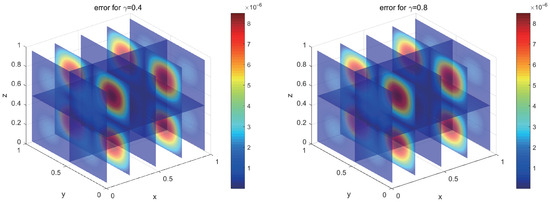
For $\gamma =0.4,0.8$, $T=1$, and $K=N=2^5$, the absolute error distribution of the numerical scheme is shown in Figure 1. This graph indicates that numerical solutions can approximate exact solutions very well.

Example 3. Case (1).

We choose $u(\mathbf{x},t)=t^{4+\gamma }sin{x}_{1}sin{x}_{2}sin{x}_3$ in (1) of 3D with $u_0(\mathbf{x},t)=0$. One can easy obtain that $f(\mathbf{x},t)$ satisfies

$$\begin{array}{c}\hfill f(\mathbf{x},t)=\left({\displaystyle \frac{\mathsf{\Gamma }(5+\gamma )}{\mathsf{\Gamma }(5)}}+6t^{4+\gamma }\right)sin{x}_{1}sin{x}_{2}sin{x}_3.\end{array}$$

In this case, we choose $K_1=1,K_2=2,K_3=3$, $\mathsf{\Omega }={[0,\pi ]}^3$, $T=1$, and $h=\Delta x_1=\Delta x_2=\Delta x_3$ with the homogeneous Dirichlet boundary condition. In order to observe the temporal convergence order, we choose $\tau =2^{-2},2^{-3},2^{-4},2^{-5}$ and $h=\tau$.

Table 5. The $Rate(\tau )$ in Example 3 for $\gamma =0.3,0.5,0.7$.

$\mathit{\tau }$	$\mathit{\gamma }=0.3$	$\mathit{Rate}(\mathit{\tau })$	$\mathit{\gamma }=0.5$	$\mathit{Rate}(\mathit{\tau })$	$\mathit{\gamma }=0.7$	$\mathit{Rate}(\mathit{\tau })$
${\displaystyle \frac{1}{4}}$	1.341644$\times {10}^{-2}$	-	3.296095$\times {10}^{-2}$	-	7.373243$\times {10}^{-2}$	-
${\displaystyle \frac{1}{8}}$	2.207850$\times {10}^{-3}$	2.603287	6.796282$\times {10}^{-3}$	2.277940	1.811728$\times {10}^{-2}$	2.024932
${\displaystyle \frac{1}{16}}$	3.449344$\times {10}^{-4}$	2.678248	1.242656$\times {10}^{-3}$	2.451317	3.824308$\times {10}^{-3}$	2.244095
${\displaystyle \frac{1}{32}}$	5.502491$\times {10}^{-5}$	2.648165	2.263858$\times {10}^{-4}$	2.456572	7.965596$\times {10}^{-4}$	2.263344

shows that $Rate(\tau )$ is an approximation of $2.3,2.5,2.7$ for $\gamma =0.7,0.5,0.3$, respectively, i.e., $Rate(\tau )=3-\gamma$, which is in complete agreement with the conclusion of Theorem 2 in time.

To observe the spatial convergence order, we set $\tau =2^{-12}$ and $h=2^{-2},2^{-3},2^{-4},2^{-5}$.

Table 6. The $Rate(h)$ in Example 3 for $\gamma =0.3,0.5,0.7$.

h	$\mathit{\gamma }=0.3$	$\mathit{Rate}(\mathit{h})$	$\mathit{\gamma }=0.5$	$\mathit{Rate}(\mathit{h})$	$\mathit{\gamma }=0.7$	$\mathit{Rate}(\mathit{h})$
${\displaystyle \frac{1}{4}}$	2.833819$\times {10}^{-3}$	-	2.619835$\times {10}^{-3}$	-	2.356383$\times {10}^{-3}$	-
${\displaystyle \frac{1}{8}}$	1.725000$\times {10}^{-4}$	4.038079	1.594906$\times {10}^{-4}$	4.037932	1.434805$\times {10}^{-4}$	4.037647
${\displaystyle \frac{1}{16}}$	1.005897$\times {10}^{-5}$	4.100041	9.301587$\times {10}^{-6}$	4.099850	8.378434$\times {10}^{-6}$	4.098031
${\displaystyle \frac{1}{32}}$	6.100803$\times {10}^{-7}$	4.043339	5.652863$\times {10}^{-7}$	4.040423	5.193794$\times {10}^{-7}$	4.011819

shows $\overline{e}(h,\tau )$ for three different values of $\gamma =0.3,0.5,0.7$. It can be seen from Table 6 that the spatial convergence order is almost $O(h^4)$ for three different values of $\gamma =0.3,0.5,0.7$, which is in complete agreement with the conclusion of Theorem 2 in space.

Case (2).

We choose $u(\mathbf{x},t)=t^{\gamma }sin{x}_{1}sin{x}_{2}sin{x}_3$ as the exact solution of the three-dimensional form of (1) with $u_0(\mathbf{x})=0$. One can easily find that $f(\mathbf{x},t)$ satisfies

$$\begin{array}{c}\hfill f(\mathbf{x},t)=[\mathsf{\Gamma }(1+\gamma )+3t^{\gamma }]sin{x}_{1}sin{x}_{2}sin{x}_3.\end{array}$$

Firstly, we choose ${\displaystyle K_1=K_2=K_3=1,\mathsf{\Omega }={[0,\pi ]}^3,T=1,h=\Delta x_1=\Delta x_2=\Delta x_3=\pi /32,K=64,128,256}$ and 512 with the homogeneous Dirichlet boundary condition to test the convergence of the numerical scheme for the nonsmooth solution.

Table 7. The $Rate(\tau )$ in Example 3 for $\gamma =0.3,0.5,0.7$.

$\mathit{\tau }$	$\mathit{\gamma }=0.3$	$\mathit{Rate}(\mathit{\tau })$	$\mathit{\gamma }=0.5$	$\mathit{Rate}(\mathit{\tau })$	$\mathit{\gamma }=0.7$	$\mathit{Rate}(\mathit{\tau })$
${\displaystyle \frac{1}{64}}$	4.148854$\times {10}^{-2}$	-	2.795845$\times {10}^{-2}$	-	1.207707$\times {10}^{-2}$	-
${\displaystyle \frac{1}{128}}$	3.701945$\times {10}^{-2}$	0.164429	2.161112$\times {10}^{-2}$	0.371510	7.896415$\times {10}^{-3}$	0.613001
${\displaystyle \frac{1}{256}}$	3.267667$\times {10}^{-2}$	0.180022	1.634605$\times {10}^{-2}$	0.402831	5.050830$\times {10}^{-3}$	0.644677
${\displaystyle \frac{1}{512}}$	2.854663$\times {10}^{-2}$	0.194940	1.215156$\times {10}^{-2}$	0.427800	3.184927$\times {10}^{-3}$	0.665260

reports that $Rate(\tau )$ is close to $0.3,0.5,0.7$ with respect to $\gamma =0.3,0.5$, and $0.7$, respectively. It is observed that the proposed scheme does not give the desired order $(3-\gamma )$ in time.

Secondly, in order to compare the effectiveness of the proposed algorithm, we choose the same graded temporal mesh parameter as Ref. [31]. Considering the high accuracy of the SFCD, we set ${\displaystyle h=\Delta x_1=\Delta x_2=\Delta x_3=\pi /32}$, which is larger than the spatial mesh size ${\displaystyle h=\Delta x_1=\Delta x_2=\Delta x_3=\pi /128}$ of [31] in the following

Table 8. Comparison of errors between the error and the time convergence orders in Table 2 of [31] (Example 1) and numerical scheme (21) for $\gamma =0.15,0.25,0.30,0.45$.

$\mathit{\gamma }$	$\mathit{\tau }$	$\overline{\mathit{e}}(\mathit{h},\mathit{\tau })$ [31]	$\mathit{Rate}(\mathit{\tau })$	$\overline{\mathit{e}}(\mathit{h},\mathit{\tau })$ (21)	$\mathit{Rate}(\mathit{\tau })$
0.15	${\displaystyle \frac{1}{4}}$	1.6300	-	2.3993$\times {10}^{-1}$	-
	${\displaystyle \frac{1}{8}}$	1.4648	0.1542	2.0201$\times {10}^{-1}$	0.2482
	${\displaystyle \frac{1}{16}}$	1.2855	0.1884	1.6400$\times {10}^{-1}$	0.3007
	${\displaystyle \frac{1}{32}}$	1.1085	0.2137	1.2852$\times {10}^{-1}$	0.3516
0.25	${\displaystyle \frac{1}{4}}$	1.4504	-	2.2866$\times {10}^{-1}$
	${\displaystyle \frac{1}{8}}$	1.1921	0.2830	1.6127$\times {10}^{-1}$	0.5037
	${\displaystyle \frac{1}{16}}$	9.3610$\times {10}^{-1}$	0.3487	1.0485$\times {10}^{-1}$	0.6211
	${\displaystyle \frac{1}{32}}$	7.1016$\times {10}^{-1}$	0.3985	6.3932$\times {10}^{-2}$	0.7137
0.30	${\displaystyle \frac{1}{4}}$	1.3351	-	2.0523$\times {10}^{-1}$
	${\displaystyle \frac{1}{8}}$	1.0315	0.3721	1.3123$\times {10}^{-1}$	0.6451
	${\displaystyle \frac{1}{16}}$	7.5521$\times {10}^{-1}$	0.4498	7.5967$\times {10}^{-2}$	0.7887
	${\displaystyle \frac{1}{32}}$	5.3135$\times {10}^{-1}$	0.5072	4.2409$\times {10}^{-2}$	0.8409
0.45	${\displaystyle \frac{1}{4}}$	1.0809	-	1.2311$\times {10}^{-1}$
	${\displaystyle \frac{1}{8}}$	6.9242$\times {10}^{-1}$	0.6425	7.4898$\times {10}^{-2}$	0.7169
	${\displaystyle \frac{1}{16}}$	4.0928$\times {10}^{-1}$	0.7586	3.8022$\times {10}^{-2}$	0.9780
	${\displaystyle \frac{1}{32}}$	2.2977$\times {10}^{-1}$	0.8329	1.6431$\times {10}^{-2}$	1.2104

.

In Table 8, we choose $r=2(2-\gamma )$ and fix the grid size ${\displaystyle h=\pi /32}$, $\gamma =0.15,0.25,0.30,0.45$, ${\displaystyle \tau =4^{-1},8^{-1},{16}^{-1},{32}^{-1},}$ respectively. From Table 8, it can be seen that the error and time convergence order of (21) are smaller and higher than those of [31], respectively.

Thirdly, in order to calculate the time convergence order of the numerical scheme (21), we choose the graded mesh parameter ${\displaystyle r=(3-\gamma )/\gamma }$.

Table 9. The $Rate(\tau )$ in Example 3 for $\gamma =0.3,0.5,0.7$.

$\mathit{\tau }$	$\mathit{\gamma }=0.3$	$\mathit{Rate}(\mathit{\tau })$	$\mathit{\gamma }=0.5$	$\mathit{Rate}(\mathit{\tau })$	$\mathit{\gamma }=0.7$	$\mathit{Rate}(\mathit{\tau })$
${\displaystyle \frac{1}{32}}$	1.284083$\times {10}^{-1}$	-	6.311899$\times {10}^{-3}$	-	2.520953$\times {10}^{-3}$	-
${\displaystyle \frac{1}{64}}$	1.999166$\times {10}^{-2}$	2.683269	1.130658$\times {10}^{-3}$	2.480911	5.370882$\times {10}^{-4}$	2.230738
${\displaystyle \frac{1}{128}}$	3.082090$\times {10}^{-3}$	2.697417	2.003439$\times {10}^{-4}$	2.496611	1.101416$\times {10}^{-4}$	2.285799
${\displaystyle \frac{1}{256}}$	4.744430$\times {10}^{-4}$	2.699602	3.543086$\times {10}^{-5}$	2.499400	2.241054$\times {10}^{-5}$	2.297110

reports that $Rate(\tau )$ is close to $(3-\gamma )$ order for $\gamma =0.3,0.5,0.7$, $\tau ={32}^{-1},{64}^{-1},{128}^{-1},{256}^{-1}$, and ${\displaystyle h=\pi /32}$.

Finally, in order to calculate the spatial convergence order of the numerical scheme (21), we choose $N=4,8,16,32,K=[N^{{\displaystyle \frac{4}{3-\gamma }}}]$.

Table 10. The $Rate(h)$ in Example 3 for $\gamma =0.3,0.5,0.7$.

h	$\mathit{\gamma }=0.3$	$\mathit{Rate}(\mathit{h})$	$\mathit{\gamma }=0.5$	$\mathit{Rate}(\mathit{h})$	$\mathit{\gamma }=0.7$	$\mathit{Rate}(\mathit{h})$
${\displaystyle \frac{1}{4}}$	3.654216 $\times {10}^0$	-	1.193667$\times {10}^{-1}$	-	2.346854$\times {10}^{-2}$	-
${\displaystyle \frac{1}{8}}$	3.787871$\times {10}^{-1}$	3.270102	9.619690$\times {10}^{-3}$	3.633267	2.017113$\times {10}^{-3}$	3.540363
${\displaystyle \frac{1}{16}}$	2.342380$\times {10}^{-2}$	4.015339	5.906558$\times {10}^{-4}$	4.025600	1.219613$\times {10}^{-4}$	4.047796
${\displaystyle \frac{1}{32}}$	1.432768$\times {10}^{-3}$	4.031098	3.543086$\times {10}^{-5}$	4.059239	7.379762$\times {10}^{-6}$	4.046706

reports that $Rate(h)$ is close to 4 for $\gamma =0.3,0.5,0.7$ in the graded mesh. This means that the order of convergence in space is independent of the parameter γ.

Example 4.

In the last example, we extend the proposed schemes to solve the time-fractional Allen–Cahn equation [39,40], which can be viewed as a kind of semi-linear TFDE appearing in the phase field modeling.

$$\begin{array}{c}\hfill \left\{\begin{array}{cc}& {}_{0}D_t^{\gamma }u(\mathbf{x},t)-{\epsilon }^2\sum _{i=1}^2{\mathsf{\partial }}_{x_i}^{2}u(\mathbf{x},t)=u(\mathbf{x},t)-u^3(\mathbf{x},t),\mathbf{x}\in \mathsf{\Omega },t\in (0,T],\hfill \\ & u(\mathbf{x},t)=0,(\mathbf{x})\in \mathsf{\partial }\mathsf{\Omega },t\in (0,T],\hfill \\ & u(\mathbf{x},0)=u_0(\mathbf{x}),(\mathbf{x})\in \mathsf{\Omega },\hfill \end{array}\right.\end{array}$$

(59)

where the exact solution of the above equation is unknown explicitly. The main difference of the proposed scheme (21) applied to Equation (59) is the need to solve the nonlinear discretized system at each time level, which is solved by the fixed-point iteration in our experiments. Moreover, since we do not theoretically investigate the convergence analysis of the proposed scheme (21) for Equation (59), here we only report some numerical results to show the wide suitability of the proposed method, which is able to solve the nonlinear TFDEs.

Case (1). The exact solution is not explicitly known: convergence accuracy. In this case, we choose $u_0(\mathbf{x})=0.5sin{x}_{1}sin{x}_2$ in (59). We specify the rectangular domain as $\mathsf{\Omega }={[0,\pi ]}^2$ and set $T=1$, ${\displaystyle \tau =1/K,h=\Delta x_1=\Delta x_2=\pi /N}$, $\epsilon =0.01$ with a homogeneous Dirichlet boundary condition. The numerical solutions with the number of time steps and spatial grid nodes as $K_{ref}=1024$ and $N_{ref}=256$ are considered as the reference solution. In

Table 11. Example 4’s $Rate(\tau )$ for $\gamma =0.3,0.5,0.7$.

h	$\mathit{\gamma }=0.3$	$\mathit{Rate}(\mathit{\tau })$	$\mathit{\gamma }=0.5$	$\mathit{Rate}(\mathit{\tau })$	$\mathit{\gamma }=0.7$	$\mathit{Rate}(\mathit{\tau })$
${\displaystyle \frac{1}{16}}$	4.091938$\times {10}^{-4}$	-	5.103915$\times {10}^{-4}$	-	4.195971$\times {10}^{-4}$	-
${\displaystyle \frac{1}{32}}$	2.017414$\times {10}^{-4}$	1.020276	2.548800$\times {10}^{-4}$	1.001785	2.215144$\times {10}^{-4}$	0.921604
${\displaystyle \frac{1}{64}}$	9.726637$\times {10}^{-5}$	1.052494	1.236686$\times {10}^{-4}$	1.043338	1.111957$\times {10}^{-4}$	0.994298
${\displaystyle \frac{1}{128}}$	4.517211$\times {10}^{-5}$	1.106508	5.768493$\times {10}^{-5}$	1.100213	5.294382$\times {10}^{-5}$	1.070567

, it is easy to see that $Rate(\tau )$ is close to 1 with respect to $\gamma =0.3,0.5,0.7$ for $K=8,16,32,64$ and $N=256$.

From Table 11, it is easy to see that the convergence order of the numerical solution is close to 1 and has not reached the (theoretical) convergence order $3-\gamma$. Considering that the analytical solution of this type of equation generally has an initial nonsmoothness, we draw a graph of the numerical solution to observe whether or not it has nonsmoothness at the initial time.

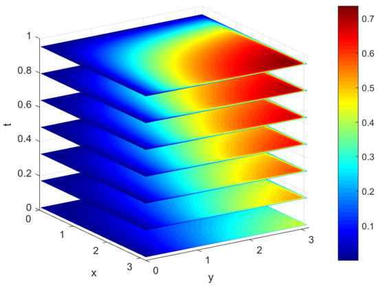
In Figure 2, the image of the numerical solution is mostly blue, and there are only a few yellow regions near the intersections of the regions at initial time $t=t_0=0$. At other times, the yellow and brown areas rapidly increase, and the blue area drastically decreases. Therefore, Figure 2 shows that the numerical solution exhibits a significant gradient over time, indicating the existence of a singularity in the solution at the initial value $t_0$. In this case, we choose ${\displaystyle t_n={(n/K)}^r}$ and ${\displaystyle r=(3-\gamma )/\gamma }$.

Table 12. Example 4’s $Rate(\tau )$ for $\gamma =0.3,0.5,0.7$.

h	$\mathit{\gamma }=0.3$	$\mathit{Rate}(\mathit{\tau })$	$\mathit{\gamma }=0.5$	$\mathit{Rate}(\mathit{\tau })$	$\mathit{\gamma }=0.7$	$\mathit{Rate}(\mathit{\tau })$
${\displaystyle \frac{1}{16}}$	3.122450$\times {10}^{-3}$	-	2.038673$\times {10}^{-3}$	-	1.486416$\times {10}^{-3}$	-
${\displaystyle \frac{1}{32}}$	4.780518$\times {10}^{-4}$	2.707439	3.428071$\times {10}^{-4}$	2.572161	2.745293$\times {10}^{-4}$	2.436806
${\displaystyle \frac{1}{64}}$	7.417093$\times {10}^{-5}$	2.688241	6.027101$\times {10}^{-5}$	2.507860	5.288236$\times {10}^{-5}$	2.376101
${\displaystyle \frac{1}{128}}$	1.148189$\times {10}^{-5}$	2.691493	1.046910$\times {10}^{-5}$	2.525326	1.006756$\times {10}^{-5}$	2.393072

reports that $Rate(\tau )$ is close to the $(3-\gamma )$-order for $\gamma =0.3,0.5,0.7$, $K=8,16,32,64$, and $N=256$.

Case (2). The exact solution is unknown: evolution of the phase field model. In this case, we choose the following initial data:

$$\begin{array}{c}\hfill \begin{array}{c}\hfill u_0=-0.8tanh(({(x_1-0.4)}^2+x_2^2-0.3^2)/\epsilon )tanh(({(x_1+0.4)}^2+x_2^2-0.3^2)/\epsilon )\\ \hfill \times tanh((x_1^2+{(x_2-0.4)}^2-0.3^2)/\epsilon )tanh((x_1^2+{(x_2+0.4)}^2-0.3^2)/\epsilon ),\end{array}\end{array}$$

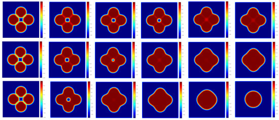
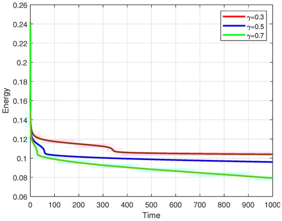
where the rectangular domain is $\mathsf{\Omega }={[-1,1]}^2$, $T=1000$, $N=128$, ${\displaystyle h=\Delta x_1=\Delta x_2=1/N}$ and $\epsilon =0.02$. Similarly, we divide the time interval $[0,T]$ into two intervals $[0,0.1]$ and $(0.1,1000]$. In the interval $[0,0.1]$ we use a graded time step ${\displaystyle (r=(3-\gamma )/\gamma )}$ to deal with the singularity problem at the initial time, while in the interval $(0.1,1000]$ we use a uniform grid with a time step of $\tau =0.01$. Figure 3 shows contour line snapshots of solutions for different fractional exponents $\gamma =0.3,0.5,0.7$. Over time, the four water droplets gradually merge into one droplet and progressively shrink. Furthermore, the larger the fractional exponent γ, the more significant the shrinkage. Figure 4 shows the change in discrete energy over time under fixed initial conditions, which is consistent with the principle of energy dissipation.

5. Conclusions

In this paper, an improved fully discrete SCFD scheme is proposed for high-dimensional TFDEs with high-order uniform temporal accuracy. An auxiliary variable is introduced to transform the high-order scheme into an equivalent form. Based on the equivalent form, we strictly establish the stability and convergence of the scheme. The improved numerical scheme ensures that the theoretical convergence accuracy at each time step is ${\displaystyle O({\tau }^{3-\gamma }+\sum _{i=1}^d\Delta x_i^4)}$ without requiring additional processing techniques. Furthermore, it is equally applicable to nonlinear TFDEs. Through experiments, we have verified that this method can be used to address the high-dimensional time-fractional Allen–Cahn equation. Traditionally, these methods were solved with Gaussian elimination, which requires computational work of ${\displaystyle O({(\prod _{i=1}^d{N}_i)}^3)}$ per time step and ${\displaystyle O({(\prod _{i=1}^d{N}_i)}^2)}$ of memory to store where $N_i$ is the number of spatial grid points in the spatial discretization of $x_i(i=1,2,\cdots ,d)$. In the future, we will utilize the block Toeplitz matrix structure of the finite difference method to construct a fast scheme for semilinear TFDEs in [41] and the theoretical analysis ideas presented in [14,42].

References

- Scher, H.; Montroll, E. Anomalous transit-time dispersion in amorphous solids. Phys. Rev. B 1975, 12, 2455–2477. [Google Scholar] [CrossRef]
- Müller, H.P.; Kimmich, R.; Weis, J. NMR flow velocity mapping in random percolation model objects: Evidence for a power-law dependence of the volume-averaged velocity on the probe-volume radius. Phys. Rev. E 1996, 54, 5278–5285. [Google Scholar] [CrossRef]
- Sathiyaraj, T.; Fečkan, M.; Wang, J.R. Synchronization of Fractional Stochastic Chaotic Systems via Mittag-Leffler Function. Fractal Fract. 2022, 6, 192. [Google Scholar] [CrossRef]
- Talebi, S.P.; Werner, S.; Mandic, D.P. Distributed Adaptive Filtering of α-Stable Signals. IEEE Signal Proc. Lett. 2018, 25, 1450–1454. [Google Scholar] [CrossRef]
- Ahmad, I.; Jan, R.; Razak, N.; Khan, A.; Abdeljawad, T. Numerical Investigation of the Dynamical Behavior of Hepatitis B Virus via Caputo-Fabrizio Fractional Derivative. Eur. J. Appl. Math. 2025, 18, 5509. [Google Scholar] [CrossRef]
- Fardi, M. A kernel-based pseudo-spectral method for multi-term and distributed order time-fractional diffusion equations. Comput. Meth. Appl. Mat. 2023, 39, 2630–2651. [Google Scholar] [CrossRef]
- Ali, U.; Iqbal, A.; Sohail, M.; Abdullah, F.A.; Khan, Z. Compact implicit difference approximation for time-fractional diffusion-wave equation. Alex. Eng. J. 2022, 61, 4119–4126. [Google Scholar] [CrossRef]
- Wang, F.; Zheng, K.; Ahmad, I.; Ahmad, H. Gaussian radial basis functions method for linear and nonlinear convection–diffusion models in physical phenomena. Open Phys. 2021, 19, 69–76. [Google Scholar] [CrossRef]
- Gao, R.M.; Li, D.F.; Li, Y.D.; Yin, Y.J. An energy-stable variable-step L1 scheme for time-fractional Navier-Stokes equations. Phys. D Nonlinear Phenom. 2024, 467, 134264. [Google Scholar] [CrossRef]
- Hou, J.; Yu, Y.G.; Wang, J.J.; Ren, H.P.; Meng, X.Y. Local analysis of L1-finite difference method on graded meshes for multi-term two-dimensional time-fractional initial-boundary value problem with Neumann boundary conditions. Comput. Math. Appl. 2024, 157, 209–214. [Google Scholar] [CrossRef]
- Seal, A.; Natesan, S. A numerical approach for nonlinear time-fractional diffusion equation with generalized memory kernel. Numer. Algorithms 2024, 97, 539–565. [Google Scholar] [CrossRef]
- Jiang, Y.B.; Chen, H.; Sun, T.; Huang, C.B. Efficient L1-ADI finite difference method for the two-dimensional nonlinear time-fractional diffusion equation. Appl. Math. Comput. 2024, 471, 128609. [Google Scholar] [CrossRef]
- Kedia, N.; Alikhanov, A.A.; Singh, V.K. Robust finite difference scheme for the non-linear generalized time-fractional diffusion equation with non-smooth solution. Math. Comput. Simul. 2024, 219, 337–354. [Google Scholar] [CrossRef]
- Cao, J.Y.; Cai, Z.N. Numerical analysis of a high-order scheme for nonlinear fractional differential equations with uniform accuracy. Numer. Math. Theor. Meth. Appl. 2021, 14, 71–112. [Google Scholar]
- Zhu, H.Y.; Xu, C.J. A fast high order method for time-fractional diffusion equation. SIAM J. Numer. Anal. 2019, 57, 2829–2849. [Google Scholar] [CrossRef]
- Podlubny, I. Fractional Differential Equations; Academic Press: New York, NY, USA, 1999. [Google Scholar]
- Roul, P.; Rohil, V. A fourth-order compact ADI scheme for solving a two-dimensional time-fractional reaction-subdiffusion equation. J. Math. Chem. 2024, 62, 2039–2055. [Google Scholar] [CrossRef]
- Irandoust-Pakchin, S.; Hossein, D.M.; Rezapour, S.; Adel, M. An efficient numerical method for the distributed-order time-fractional diffusion equation with the error analysis and stability properties. Numer. Methods Partial Differ. Equ. 2025, 48, 2743–2765. [Google Scholar] [CrossRef]
- Chen, L.S.; Wang, Z.B.; Vong, S.W. A second-order weighted ADI scheme with nonuniform time grids for the two-dimensional time-fractional telegraph equation. J. Appl. Math. Comput. 2024, 70, 1–18. [Google Scholar] [CrossRef]
- Huang, Y.C.; Lei, S.L. Fast solvers for finite difference scheme of two-dimensional time-space fractional differential equations. Numer. Algorithms 2020, 84, 37–62. [Google Scholar] [CrossRef]
- Alikhanov, A.A.; Huang, C.M. A high-order L2 type difference scheme for the time-fractional diffusion equation. Appl. Math. Comput. 2021, 411, 126545. [Google Scholar] [CrossRef]
- Zhang, X.D.; Feng, Y.L.; Luo, Z.Y.; Liu, J. A spatial sixth-order numerical scheme for solving fractional partial differential equation. Appl. Math. Lett. 2025, 159, 109265. [Google Scholar] [CrossRef]
- Liu, Z.G.; Li, X.L.; Zhang, X.H. A fast high-order compact difference method for the fractal mobile/immobile transport equation. Int. J. Comput. Math. 2020, 97, 1860–1883. [Google Scholar] [CrossRef]
- He, M.Y.; Liao, W.Y. A compact ADI finite difference method for 2D reaction-diffusion equations with variable diffusion coefficients. J. Comput. Appl. Math. 2024, 436, 115400. [Google Scholar] [CrossRef]
- Fu, H.F.; Zhang, B.Y.; Zheng, X.C. A high-order two-grid difference method for nonlinear time-fractional biharmonic problems and its unconditional α-robust error estimates. J. Sci. Comput. 2023, 96, 54. [Google Scholar] [CrossRef]
- Xu, D.; Qiu, W.L.; Guo, J. A compact finite difference scheme for the fourth-order time-fractional integro-differential equation with a weakly singular kernel. Numer. Methods Partial Differ. Equ. 2020, 36, 439–458. [Google Scholar] [CrossRef]
- Wang, Y.M.; Ren, L. A high-order L2-compact difference method for Caputo-type time-fractional sub-diffusion equations with variable coefficients. Appl. Math. Comput. 2019, 342, 71–93. [Google Scholar] [CrossRef]
- Kopteva, N. Error analysis of an L2-type method on graded meshes for semilinear subdiffusion equations. Appl. Math. Lett. 2025, 160, 109306. [Google Scholar] [CrossRef]
- Toprakseven, Ş. A weak Galerkin finite element method on temporal graded meshes for the multi-term time fractional diffusion equations. Comput. Math. Appl. 2022, 128, 108–120. [Google Scholar] [CrossRef]
- Zhao, Y.-L.; Gu, X.-M.; Ostermann, A. A preconditioning technique for an all-at-once system from Volterra subdiffusion equations with graded time steps. J. Sci. Comput. 2021, 88, 11. [Google Scholar] [CrossRef]
- Zhou, Z.Y.; Zhang, H.X.; Yang, X.H. H1-norm error analysis of a robust ADI method on graded mesh for three-dimensional subdiffusion problems. Numer. Algorithms 2024, 96, 1533–1551. [Google Scholar] [CrossRef]
- Qiao, H.L.; Cheng, A.J. A fast modified L1 finite difference method for time fractional diffusion equations with weakly singular solution. J. Appl. Math. Comput. 2024, 70, 3631–3660. [Google Scholar] [CrossRef]
- Zheng, Z.Y.; Wang, Y.M. Fast high-order compact finite difference methods based on the averaged L1 formula for a time-fractional mobile-immobile diffusion problem. J. Sci. Comput. 2024, 99, 43. [Google Scholar] [CrossRef]
- Cao, D.W.; Chen, H. Error analysis of a finite difference method for the distributed order sub-diffusion equation using discrete comparison principle. Math. Comput. Simul. 2023, 211, 109–117. [Google Scholar] [CrossRef]
- Cao, J.Y.; Wang, Z.Q.; Wang, Z.Q. Stability and convergence analysis for a uniform temporal high accuracy of the time-fractional diffusion equation with 1D and 2D spatial compact finite difference method. AIMS Math. 2024, 9, 14697–14730. [Google Scholar] [CrossRef]
- Zhang, X.; Gu, X.-M.; Zhao, Y.-L. Two fast finite difference methods for a class of variable-coefficient fractional diffusion equations with time delay. Commun. Nonlinear Sci. Numer. Simul. 2025, 140, 108358. [Google Scholar] [CrossRef]
- Zhang, Y.N.; Sun, Z.Z. Error analysis of a compact ADI scheme for the 2D fractional subdiffusion equation. J. Sci. Comput. 2014, 59, 104–128. [Google Scholar] [CrossRef]
- Sun, H.; Sun, Z.Z. A fast temporal second-order compact ADI difference scheme for the 2D multi-term fractional wave equation. Numer. Algorithms 2021, 86, 761–797. [Google Scholar] [CrossRef]
- Liao, H.L.; Tang, T.; Zhou, T. An energy stable and maximum bound preserving scheme with variable time steps for time fractional Allen–Cahn equation. SIAM J. Sci. Comput. 2021, 43, A3503–A3526. [Google Scholar] [CrossRef]
- Wang, J.; Chen, X.J.; Chen, J.H. A high-precision numerical method based on spectral deferred correction for solving the time-fractional Allen-Cahn equation. Comput. Math. Appl. 2025, 180, 1–27. [Google Scholar] [CrossRef]
- Zhao, Y.Q.; Tang, Y.B. Critical behavior of a semilinear time fractional diffusion equation with forcing term depending on time and space. Chaos Solitons Fract. 2024, 178, 114309. [Google Scholar] [CrossRef]
- Gu, X.-M.; Wu, S.-L. A parallel-in-time iterative algorithm for Volterra partial integro-differential problems with weakly singular kernel. J. Comput. Phys. 2020, 417, 109576. [Google Scholar] [CrossRef]
Disclaimer/Publisher’s Note: The statements, opinions and data contained in all publications are solely those of the individual author(s) and contributor(s) and not of MDPI and/or the editor(s). MDPI and/or the editor(s) disclaim responsibility for any injury to people or property resulting from any ideas, methods, instructions or products referred to in the content. |
© 2025 by the authors. Licensee MDPI, Basel, Switzerland. This article is an open access article distributed under the terms and conditions of the Creative Commons Attribution (CC BY) license (https://creativecommons.org/licenses/by/4.0/).