1. Introduction
The utilisation of symmetry as a means to identify conserved quantities has emerged as a contemporary approach to studying the conservation of constrained mechanical systems. This methodology has garnered significant attention within the realm of analytical mechanics, a field that is undergoing rapid advancements. The classical symmetry encompasses Noether symmetry [
1], Lie symmetry [
2], and Mei symmetry [
3]. Noether’s theorem has a series of findings in analytical mechanics [
4,
5]. In 2017, Zhai and Zhang [
6] proposed the Noether theorem with delay on time scales and Song [
7] studied the Noether theorem of non-standard system. Recently, Anerot and Cresson [
8] carried out numerical simulations of the Noether theorems on time scales. Furthermore, Noether-type adiabatic invariants and Herglotz-type Noether theorems were studied in [
9,
10,
11].
Time-scale theory is a mathematical theory proposed by German scholar Hilger [
12] in 1988. It is frequently the case that the initiation of a study on one time scale can yield divergent results when conducted on a different time scale. The time-scale theory has the capacity to unify discrete and continuous conditions for study, thus facilitating the revelation of the similarities and differences between discrete and continuous conditions, as well as providing a clearer and more accurate understanding of the essential problems of complex dynamical systems. The superiority of fractional calculus over integer models in the analysis of complex systems is attributable to its unique memory and non-locality. Consequently, fractional differential equations are capable of providing more accurate descriptions of a wider range of practical problems than integer differential equations. A series of findings have been obtained in the research concerning fractional calculus [
13,
14] and time-scale calculus [
15,
16,
17]. Fractional time-scales calculus has also achieved some results; these include principles and inequalities [
18] and dynamical Equations [
19]. However, the number of studies examining symmetries on fractional time scales is limited; indeed, only a small number of studies [
20,
21] address the topic.
The non-standard Lagrangian has been employed for the modelling of non-linear, non-conservative dynamical systems, and has been applied to dissipative systems [
22], classical system dynamics [
23], and so forth in recent years. Birkhoffian mechanics [
24] represents a significant theoretical framework within the broader domain of Hamiltonian mechanics, characterised by its notable degree of generalisation. Consequently, the investigation of the symmetry inherent in non-standard Birkhoffian systems operating on fractional time scales assumes considerable theoretical and practical importance. The symmetry of non-standard systems on fractional time scales has not been studied hitherto. This paper will investigate the Noether symmetries of non-standard Birkhoffian systems based on Caputo delta derivatives, which leads to a more widely applicable method for solving the equations of complex systems.
The following description outlines the arrangement of the text: initially, we list a number of definitions and lemmas that are deemed essential for this paper. Then, in
Section 3, we derive fractional non-standard equations of motion with Caputo
derivatives and then degenerate them to the fractional order, time scale order, and the classical case. Subsequently, we derive their Noether identities and conserved quantities in
Section 4, which lead to Noether theorems. Then, three illustrative examples are presented to demonstrate the accuracy in
Section 5. Finally, we conclude the article and present some perspectives.
2. Preliminaries
In order to facilitate comprehension, the following definition of time scale is listed.
A time scale is an arbitrary non-empty closed subset of the real numbers. Thus, the real numbers , the integers , and the natural numbers are examples of time scales. For , we define the forward jump operator and the backward jump operator . Suppose that the function , if given any , there is a neighbourhood U of t satisfying for all , then is called the delta derivative of f at . A function is called rd-continuous at right-dense points and its left-sided limits exist at left-dense points. The set of all rd-continuous functions in is donoted , and the set of delta differentiable functions in with continuous delta derivatives is donated .
More introductions of time scales can be found in references [
25,
26,
27]. Next, we focus on the main definitions [
28,
29,
30] and remarks [
31,
32,
33] of the fractional time scales needed for this article.
Definition 1. Let , t,, defining rd-continuous functions :where . Definition 2. Let , , and the left and right Riemann–Liouville Δ integrals are Remark 1. Let , we can get . If , we can obtain Definition 3. Let , for , and the left and right Caputo Δ derivatives arewhere is the left Riemann–Liouville Δ derivative and is the right Riemann–Liouville Δ derivative. Lemma 1. If , are delta differentiable, then the Leibniz formula for the delta derivative is If and are delta differentiable, the following formulas represent the integration of fractional time scales by parts: Lemma 2. Let , , holds for with iff is a constant on .
The left Caputo derivative is denoted as and the right Riemann–Liouville derivative is denoted as in the following text.
3. Differential Equations of Motion
3.1. Exponential Birkhoffian
Assume that the Pfaff action for the dynamical system based on the fractional exponential Birkhoffian on time scales is
where
is the Birkhoffian variable,
are Birkhoffian functions and
is the Birkhoffian,
.
The Pfaff–Birkhoff principle is
which satisfies commutative conditions
and boundary conditions
Substituting Equation (
11) into Equation (
12), we get
According to Equation (
9), and then by commutative conditions (
13) and boundary conditions (
14), we get
By Lemma 2, taking the delta derivative of Equation (
17), we get
Equation (
18) is the fractional differential equation of motion based on the exponential Birkhoffian on time scales. The differential equation is a coupling term on fractional time scales that unifies the constraints and maintains its symmetry for both non-holonomic and complex constrained systems. The non-standard equations of the Birkhoffian system can be employed for the modelling of non-conservative dynamical systems, where the Birkhoffian
B can generally be used to represent the energy. The same goes for the next two cases.
Remark 2. If , Equation (18) reduces to the equation of motion based on the exponential Birkhoffian on time scales If , Equation (18) reduces to the fractional equation of motion based on the exponential Birkhoffian If , , Equation (18) reduces to the classical differential equation of motion based on the exponential Birkhoffian The result is consistent with that in reference [24]. 3.2. Logarithmic Birkhoffian
Assume that the Pfaff action for the dynamical system based on the fractional logarithmic Birkhoffian on time scales is
where
is the Birkhoffian variable,
are Birkhoffian functions, and
is the Birkhoffian,
.
The Pfaff–Birkhoff principle is
which satisfies commutative conditions
and boundary conditions
Substituting Equation (
22) into Equation (
23), we have
According to Equation (
9), and then by commutative conditions (
24) and boundary conditions (
25), we get
By Lemma 2, taking the delta derivative of Equation (
28), we get
Equation (
29) is the fractional differential equation of motion based on the logarithmic Birkhoffian on time scales.
Remark 3. If , Equation (29) reduces to the equation of motion based on the logarithmic Birkhoffian on time scales If , Equation (29) reduces to the fractional equation of motion based on the logarithmic Birkhoffian If , , Equation (29) reduces to the classical differential equation of motion based on the logarithmic Birkhoffian The result is consistent with that in reference [24]. 3.3. Power Birkhoffian
Assume that the Pfaff action for the dynamical system based on the fractional power Birkhoffian on time scales is
where
is the Birkhoffian variable,
are Birkhoffian functions, and
is the Birkhoffian,
.
The Pfaff–Birkhoff principle is
which satisfies commutative conditions
and boundary conditions
Substituting Equation (
33) into Equation (
34), we have
According to Equation (
9), and then by commutative conditions (
35) and boundary conditions (
36), we get
By Lemma 2, taking the delta derivative of Equation (
39), we have
Equation (
40) is the fractional differential equation of motion based on the power Birkhoffian on time scales.
Remark 4. If , Equation (40) reduces to the equation of motion based on the power Birkhoffian on time scales If , Equation (40) reduces to the fractional equation of motion based on the power Birkhoffian If , , Equation (40) reduces to the classical differential equation of motion based on the power Birkhoffian The result is consistent with that in reference [24]. The introduction of fractional theory allows the equations to be degraded to integer order models. The time-scale theory enables equations to degenerate into discrete case, where it is constructed in a way that avoids the numerical dissipation caused by artificial discrete motions, and inherits realistically the geometrical properties of the solution of a continuous system, such as the structure-preserving system.
4. Noether’s Theorem
We introduce the infinitesimal transformation
where
is the infinitesimal parameter and
,
are infinitesimal generators of the transformation. Define the mapping
as a new time scale
and as a strictly increasing
function whose forward jump operator is
, and whose corresponding
derivative is
.
4.1. Exponential Birkhoffian System
Definition 4. For arbitrary closed interval , ifthen it is claimed that action Equation (11) is invariant under the general infinitesimal transformation. If Equation (
11) is invariant under the transformation, then the generators
,
satisfy the Noether identity
Proof. Expanding Equation (
45), we have
Since
, Equation (
47) is equal to
Taking the derivative of Equation (
48) with respect to
and put
, then we obtain Equation (
46). □
Theorem 1. If Equation (11) is invariant under Definition 4, thenis a Noether conserved quantity, where . Proof. Taking the delta derivative of Equation (
49), making use of Equations (
18) and (
46), we have
Hence, Equation (
49) is a Noether conserved quantity of the exponential Birkhoffian system. □
Remark 5. If , Noether identity (46) reduces toand the Noether conserved quantity (49) reduces to If , Noether identity (46) reduces toand the Noether conserved quantity (49) reduces to 4.2. Logarithmic Birkhoffian System
Definition 5. For any , ifthen it is claimed that action Equation (22) is invariant under the general infinitesimal transformation. If Equation (
22) is invariant under the transformation, then the generators
,
satisfy the Noether identity
Proof. Expanding Equation (
55), we have
Since
, Equation (
57) is equal to
Taking the derivative of Equation (
58) with respect to
and put
, then we obtain Equation (
56). □
Theorem 2. If Equation (22) is invariant under Definition 5, thenis a Noether conserved quantity. Proof. Taking the delta derivative of Equation (
59), making use of Equations (
29) and (
56), we have
Hence, Equation (
59) is a Noether conserved quantity of the exponential Birkhoffian system. □
Remark 6. If , Noether identity (56) reduces toand the Noether conserved quantity (59) reduces to If , Noether identity (56) reduces toand the Noether conserved quantity (59) reduces to 4.3. Power Birkhoffian System
Definition 6. For any , ifthen it is claimed that the action Equation (33) is invariant under the general infinitesimal transformation. If Equation (
33) is invariant under the transformation, then the generators
,
satisfy the Noether identity
Proof. Expanding Equation (
65), we have
Since
, Equation (
67) is equal to
Taking the derivative of Equation (
68) with respect to
and put
, then we get Equation (
66). □
Theorem 3. If Equation (33) is invariant under Definition 6, thenis a Noether conserved quantity. Proof. Taking the delta derivative of Equation (
69), making use of Equations (
40) and (
66), we have
Hence, Equation (
69) is a Noether conserved quantity of the power Birkhoffian system. □
Remark 7. If , Noether identity (66) reduces toand the Noether conserved quantity (69) reduces to If , Noether identity (66) reduces toand the Noether conserved quantity (69) reduces to 5. Examples
Considering the fractional Hojman–Urrutia model [
34,
35] on time scales, where
, the Birkhoffian and Birkhoffian functions are
Next, we investigate Noether symmetries under exponential, logarithmic, and power Birkhoffian separately.
For exponential Birkhoffian, the Pfaff action is
Equation (
18) gives the equation of motion:
The Noether identity Equation (
46) gives
Equation (
78) can obtain the following solution
Theorem 1 gives the following conserved quantity
where
,
.
For logarithmic Birkhoffian, the Pfaff action is
Equation (
29) gives the equation of motion:
The Noether identity Equation (
56) gives
Equation (
83) can also obtain the solution (
79). Theorem 2 gives the following conserved quantity
where
.
For power Birkhoffian, the Pfaff action is
Equation (
40) gives the equation of motion:
The Noether identity Equation (
66) gives
Equation (
87) can also obtain the solution (
79). By Theorem 3, we have the following Noether conserved quantity
If
,
,
and
and
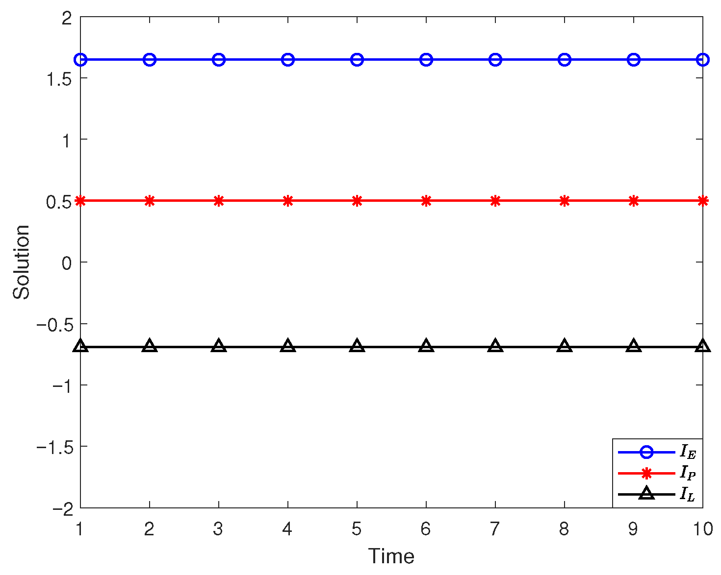
. Given initial conditions
,
,
,
, then we can get the following simulation
Figure 1.
The results indirectly prove the findings in reference [
21].
6. Conclusions
The application of fractional theory and time-scale theory to the study of dynamical problems has resulted in the establishment of a more widely appropriate fractional time-scales model. Noether’s theorem for non-standard Birkhoffian system under Caputo derivatives is discussed in the paper and several special cases are given; some of the special case results are consistent with the original results and some are new. Given the unifying and extensibility features exhibited by time-scale theory, the methods and results presented in this paper have the potential for a much wider range of applications that can be extended to different complex systems. Non-standard functions can be used to model non-linear, non-conservative dynamical systems. However, it is clear that further refinement is required in subsequent research, for example in terms of the specific physical meaning of conserved quantities in practical problems.
The investigation of the fractional time-scales theory is still in its infancy, with a considerable amount of work yet to be completed. For instance, there are the Lie symmetry and Hojman conserved quantities, the Mei symmetry and Mei conserved quantities on fractional time scales, methods for extending the theory to non-holonomic systems, and so forth.
Author Contributions
Z.W.: Conceptualisation (equal); Methodology (equal); Validation (equal); Writing—original draft (lead); Writing—review and editing (equal). C.S.: Conceptualisation (equal); Methodology (equal); Formal analysis (equal); Validation (equal); Writing—review and editing (equal); Funding acquisition (lead); Project administration (lead); Supervision (lead). All authors have read and agreed to the published version of the manuscript.
Funding
This work was supported by the National Natural Science Foundation of China (Grant Nos. 12172241 and 12272248), the Qing Lan Project of Jiangsu Province, and the Innovation Program for Postgraduate in Higher Education Institutions of Jiangsu Province (Grant No. KYCX24_3410).
Data Availability Statement
The original contributions presented in this study are included in the article. Further inquiries can be directed to the corresponding author.
Conflicts of Interest
The authors declare no conflicts of interest.
References
- Noether, A.E. Invariante variationsproblem. Nachr. Akad. Wiss. Göttingen Math. Phys. 1918, 2, 235–257. [Google Scholar]
- Mei, F.X. Application of Lie Groups and Lie Algebras to Binding Systems; Science Press: Beijing, China, 1999. [Google Scholar]
- Mei, F.X. Form invariance of Lagrange system. J. B Univ. Technol. 2000, 9, 120–124. [Google Scholar]
- Mei, F.X. Analytical Mechanics; Beijing Institute of Technology Press: Beijing, China, 2013. [Google Scholar]
- Mei, F.X. Symmetry and Conserved Quantity of Constrained Mechanical Systems; Beijing Institute of Technology Press: Beijing, China, 2004. [Google Scholar]
- Zhai, X.H.; Zhang, Y. Noether theorem for non-conservative systems with time delay on time scales. Commun. Nonlinear Sci. Numer. Simul. 2017, 52, 32–43. [Google Scholar] [CrossRef]
- Song, J.; Zhang, Y. Noether symmetry and conserved quantity for dynamical system with non-standard Lagrangians on time scales. Chin. Phys. B 2017, 26, 084501. [Google Scholar] [CrossRef]
- Anerot, B.; Cresson, J.; Belgacem, K.H. Noether’s-type theorems on time scales. J. Math. Phys. 2020, 61, 113502. [Google Scholar] [CrossRef]
- Song, C.J.; Hou, S. Noether-type adiabatic invariants for constrained mechanics systems on time scales. Chin. J. Theor. Appl. Mech. 2024, 56, 2397–2407. [Google Scholar]
- Deng, Y.Y.; Zhang, Y. Herglotz type Noether theorems of nonholonomic systems with generalized fractional derivatives. Theor. Appl. Mech. Lett. 2025, 15, 100574. [Google Scholar] [CrossRef]
- Zhang, Y. Canonical equations for generalized Chaplygin systems and Herglotz-type Noether theorems. Acta Mech. 2025, 236, 1061–1070. [Google Scholar] [CrossRef]
- Hilger, S. Ein Maßkettenkalkiil mit Anwendung auf Zentrumsmannigfaltigkeiten. Ph.D. Thesis, Universität Würzburg, Würzburg, Germany, 1988. [Google Scholar]
- Wu, G.C.; Baleanu, D. Discrete fractional logistic map and its chaos. Nonlinear Dyn. 2014, 75, 283–287. [Google Scholar] [CrossRef]
- Wang, X.; Xu, H. Numerical analysis and comparison of fractional physics-informed neural networks in unsaturated flow process. Commun. Nonlinear Sci. Numer. Simul. 2025, 147, 108833. [Google Scholar] [CrossRef]
- Goktas, S.; Belveren, B.; Gurefe, Y. Some extended properties and applications of multiplicative time scale calculus. J. Funct. Space 2025, 1, 3330782. [Google Scholar] [CrossRef]
- Song, C.J.; Cheng, Y. Noether’s theorems for nonshifted dynamic systems on time scales. Appl. Math. Comput. 2020, 374, 125086. [Google Scholar] [CrossRef]
- Wu, J.; Song, Q.; Liu, Y. Lagrange stability of quaternion-valued neural networks with mixed delays on time scales. Neurocomputing 2025, 618, 129086. [Google Scholar] [CrossRef]
- Benkhettou, N.; Hammoudi, A.; Torres, D.F.M. Existence and uniqueness of solution for a fractional R-L initial value problem on time scales. J. King Saud Univ. Sci. 2016, 28, 87–92. [Google Scholar] [CrossRef]
- Kheira, M.; Torres, D.F.M. Generalized fractional operators on time scales with application to dynamic equations. Eur. Phys. J. Spec. Top. 2017, 226, 3489–3499. [Google Scholar]
- Tian, X.; Zhang, Y. Fractional time-scales Noether theorem with Caputo derivatives for Hamiltonian systems. Appl. Math. Comput. 2021, 339, 125753. [Google Scholar]
- Tian, X.; Zhang, Y. Caputo type fractional time-scales Noether theorem of Birkhoffian systems. Acta Mech. 2022, 233, 4487–4503. [Google Scholar] [CrossRef]
- Song, J.; Zhang, Y. Routh method of reduction for dynamical systems with nonstandard Lagrangians on time scales. Indian J. Phys. 2020, 94, 501–506. [Google Scholar] [CrossRef]
- Zhang, Y.; Zhou, X.S. Noether theorem and its inverse for nonlinear dynamical systems with non-standard Lagrangians. Nonlinear Dyn. 2016, 84, 1867–1876. [Google Scholar] [CrossRef]
- Zhang, L.J.; Zhang, Y. Non-standard Birkhoffian dynamics and its Noether’s theorems. Commun. Nonlinear Sci. Numer. Simul. 2020, 91, 105435. [Google Scholar] [CrossRef]
- Bohner, M.; Peterson, A. Dynamic Equations on Time Scales; Birkhäuser: Cham, Switzerland, 2001. [Google Scholar]
- Bohner, M.; Georgiev, S.G. Multivariable Dynamic Calculus on Time Scales; Springer: Berlin, Germany, 2016. [Google Scholar]
- Martins, N.; Torres, D.F.M. Calculus of variations on time scales with nabla derivatives. Nonliner Anal-Model. 2009, 71, e763–e773. [Google Scholar] [CrossRef]
- Georgiev, S.G. Fractional Dynamic Calculus and Fractional Dynamic Equations on Time Scales; Springer: Berlin, Germany, 2018. [Google Scholar]
- Anastassiou, G.A. Foundations of nabla fractional calculus on time scales and inequalities. Comput. Math. Appl. 2010, 59, 3750–3762. [Google Scholar] [CrossRef]
- Anastassiou, G.A. Principles of delta fractional calculus on time scales and inequalities. Math. Comp. Model. Dyn. 2010, 52, 556–566. [Google Scholar] [CrossRef]
- Podlubny, I. Fractional Differential Equation; Academic Press: New York, NY, USA, 1999. [Google Scholar]
- Atici, F.M.; Eloe, P.M. A transform method in discrete fractional calculus. Int. J. Differ. Equ. 2007, 2, 165–176. [Google Scholar]
- Anastassiou, G.A. Nabla discrete fractional calculus and nabla inequalities. Math. Comp. Model. Dyn. 2010, 51, 562–571. [Google Scholar] [CrossRef]
- Mei, F.X.; Shi, R.C.; Zhang, Y.F.; Wu, H.B. Dynamics of Birkhoffian System; Beijing Institute of Technology Press: Beijing, China, 1996. [Google Scholar]
- Hojman, S.; Urrutia, L.F. On the inverse problem of the calculus of variations. J. Math. Phys. 1981, 22, 1896–1903. [Google Scholar] [CrossRef]
| Disclaimer/Publisher’s Note: The statements, opinions and data contained in all publications are solely those of the individual author(s) and contributor(s) and not of MDPI and/or the editor(s). MDPI and/or the editor(s) disclaim responsibility for any injury to people or property resulting from any ideas, methods, instructions or products referred to in the content. |
© 2025 by the authors. Licensee MDPI, Basel, Switzerland. This article is an open access article distributed under the terms and conditions of the Creative Commons Attribution (CC BY) license (https://creativecommons.org/licenses/by/4.0/).


