Finite Element Simulation for Fractional Allen–Cahn Equation with Regularized Logarithmic Free Energy

Abstract

This paper is focused on developing a Galerkin finite element framework for the fractional Allen–Cahn equation with regularized logarithmic potential over the ${\mathbb{R}}^d$ ($d=1,2,3$) domain, where the regularization of the singular potential extends beyond the classical double-well formulation. A fully discrete finite element scheme is developed using a k-th-order finite element space for spatial approximation and a backward Euler scheme for the temporal discretization of a regularized system. The existence and uniqueness of numerical solutions are rigorously established by applying Brouwer’s fixed-point theorem. Moreover, the proposed numerical framework is shown to preserve the discrete energy dissipation law analytically, while a priori error estimates are derived. Finally, numerical experiments are conducted to verify the theoretical results and the inherent physical property, such as phase separation phenomenon and coarsening processes. The results show that the fractional Allen–Cahn model provides enhanced capability in capturing phase transition characteristics compared to its classical equation.

1. Introduction

The main objectives of this article are to propose a finite element method and conduct its numerical analysis for the fractional Allen–Cahn equation with regularized logarithmic free energy:

$$\begin{array}{cc}\hfill \left(a\right)& u_t+{\epsilon }^2{(-\mathrm{\Delta })}^{r}u+{\mathrm{\Psi }}^{\prime }\left(u\right)=0\mathrm{in}{\mathrm{\Omega }}_T:=\mathrm{\Omega }\times (0,T),\hfill \\ \hfill \left(b\right)& u(x,0)=u^0\mathrm{in}\mathrm{\Omega },\hfill \\ \hfill \left(c\right)& {u|}_{\partial \mathrm{\Omega }}=0\mathrm{on}\partial \mathrm{\Omega }\times (0,T),\hfill \end{array}$$

(1)

which characterizes the coarsening dynamics with long-range interactions of a two-phase system in a phase field approach. This formulation extends classical phase field theories to nonlocal phenomena [1,2,3,4,5,6] while also enabling applications in biological systems [7,8], nuclear morphology [9], and droplet dynamics [10,11]. Here, $\mathrm{\Omega }\subset {\mathbb{R}}^d$ as $d=1,2,3$ is a bounded and convex domain with smooth boundary $\partial \mathrm{\Omega },$ and ${\epsilon }^2$ serves as the diffusion coefficient. The unknown $u\in [-1,1]$—the non-conserved order parameter—quantifies the normalized atomic density difference between coexisting phases in the two-phase system. For instance, $u=\pm 1$ corresponds to the pure phases A and B, respectively; ${(-\mathrm{\Delta })}^r$ with $0<r\le 1$ is the fractional Laplace operator; and $\mathrm{\Psi }\left(u\right):[-1,1]\to \mathbb{R}$ is the regularized logarithmic free energy functional, which is technically designed to effectively approximate the logarithmic potential $\widehat{\mathrm{\Psi }}\left(u\right)$ given by

$$\begin{array}{cc}\hfill & \widehat{\mathrm{\Psi }}\left(u\right)={\displaystyle \frac{\theta }{2}}[(1+u)ln(1+u)+(1-u)ln(1-u)]+{\displaystyle \frac{\omega }{2}}(1-u^2)\hfill \end{array}$$

(2)

with the absolute and critical temperatures $\theta$ and $\omega$ satisfying $0<\theta <\omega .$ In Section 2, We shall give a detailed discussion on the properties of the fractional Laplace operator ${(-\mathrm{\Delta })}^r$ and how the regularization removes the weak singularity of the logarithmic potential $\widehat{\mathrm{\Psi }}\left(u\right)$ at $u=\pm 1.$

The above system constitutes a natural generalization of the well-known and extensively studied Allen–Cahn equation with classical double-well potentials. More precisely, when an $r=1,$ system (1a) reduces to the Allen–Cahn equation [12,13], and when $\theta \to \omega$,

$$\begin{array}{c}\hfill \widehat{\mathrm{\Psi }}\left(u\right)\approx {\displaystyle \frac{\theta }{12}}{u}^4-{\displaystyle \frac{(\omega -\theta )}{2}}{u}^2+{\displaystyle \frac{\omega }{2}}.\end{array}$$

Using the Taylor expansion of $\widehat{\mathrm{\Psi }}\left(u\right)$ at $u=0$, the logarithmic free energy (2) thus reduces to the classical double-well model in the form of a quartic polynomial, widely used in the literature.

However, the logarithmic potential was originally introduced to model the entropic contributions to free energy in thermodynamic systems [12,13,14]. Its formulation preserves the underlying thermodynamics of phase separation more rigorously than polynomial approximations, which may not fully capture entropic effects in certain systems. Moreover, long-range interparticle interactions require nonlocal operators for physical accuracy [15,16,17,18,19,20], and the fractional Laplacian operator stands out as a favorable choice due to its role as a natural extension of the classical Laplacian and its retention of desirable properties of classical elliptic operators, such as self-adjointness and positivity. Motivated by these considerations, we aim to establish a computational framework for the fractional Allen–Cahn equation with a regularized logarithmic free energy, which simultaneously ensures thermodynamic consistency and accurately captures the dynamics of nonlocal interactions.

In the literature, numerical methods for the fractional Allen–Cahn equation have been extensively studied. Specifically, Zhai et al. [21,22] adopted the spectral method to develop an efficient algorithm, while Cui et al. [23,24] employed finite-difference-like schemes. For finite element simulations, relevant works can be found in [2,4,25,26]. It is worth noting that all these studies are based on the classical double-well potential. Unlike the extensive study on the solvability theory and the numerical simulations for the (fractional) Allen–Cahn equation with polynomial potential, there are few studies on the solvability theory of the fractional Allen–Cahn model with logarithmic potential, owing to the computing challenges from the nonlocality of the fractional Laplacian and the weak singularity of the logarithmic potential.

In this article, we propose a finite element method for (1), following the idea of regularization [27,28], whereby weak singularities may be reduced and regularized potentials can successively approximate the logarithmic counterpart. We then prove the existence and uniqueness, the energy decay property, and the optimal convergence rate for the finite element solution, using the Brouwer fixed-point theorem. Numerical experiments were conducted to verify the theoretical findings and demonstrate our method’s better applicability compared to traditional numerical models.

The remainder of this article is organized as follows. Section 2 reviews the basic properties of the fractional Laplacian and the regularized logarithmic potential. Section 3 develops a fully discrete finite element scheme and establishes its solvability. Section 4 provides a rigorous analysis of energy dissipation laws and convergence properties. Finally, Section 5 presents numerical experiments demonstrating theoretical findings and investigating physical characteristics of the proposed framework.

2. Preliminaries

In this section, we shall review the essential properties for the fractional Laplacian operator ${(-\mathrm{\Delta })}^r(0<r<1)$ [29,30] and the regularization of the logarithmic potential (2) [27].

Assume that $\mathcal{S}\left(\mathbb{R}\right)$ as $d=1,2,3$ is the Schwartz space consisting of all rapidly decaying functions. Let ${(-\mathrm{\Delta })}^r$ be a fractional Laplacian operator of order r defined as $0<r<1$, for $u\left(x\right)\in \mathcal{S}\left(\mathbb{R}\right)$:

$$\begin{array}{c}\hfill {(-\mathrm{\Delta })}^{r}u\left(x\right):={\displaystyle \frac{4^{r}r\mathrm{\Gamma }(\frac{d}{2}+r)}{{\pi }^{d/2}\mathrm{\Gamma }(1-r)}}\underset{ϵ\to 0}{lim}{\int }_{{\mathbb{R}}^d\setminus B(x,ϵ)}{\displaystyle \frac{u\left(x\right)-u\left(y\right)}{{|x-y|}^{d+2r}}}dy,\end{array}$$

(3)

where $B(x,ϵ)$ denotes the $ϵ$-ball of ${\mathbb{R}}^d$ centered at x, and $C_r={\displaystyle \frac{4^{r}r\mathrm{\Gamma }(\frac{d}{2}+r)}{{\pi }^{d/2}\mathrm{\Gamma }(1-r)}}.$ We understand that ${(-\mathrm{\Delta })}^r$ reduces to the Laplacian operator $-\mathrm{\Delta }$ as $r\to 1$.

To establish the variational framework for model (1), we shall define the fractional Sobolev space, which is closely related to the fractional Laplace operator ${(-\mathrm{\Delta })}^r$.

Definition 1

([29,30]). Let the space $L^2\left({\mathbb{R}}^d\right)$ be endowed with its standard scalar product

$$(u,v)={\int }_{{\mathbb{R}}^d}u\left(x\right)v\left(x\right)dx,\mathrm{for}u,v\in L^2\left({\mathbb{R}}^d\right)$$

and the induced norm ${\parallel u\parallel }_{L^2\left({\mathbb{R}}^d\right)}^2=(u,u).$ We define the fractional Sobolev space $H^r\left({\mathbb{R}}^d\right)$ as

$$H^r\left({\mathbb{R}}^d\right):=\left\{v\in L^2\left({\mathbb{R}}^d\right):{\displaystyle \frac{{|v\left(x\right)-v\left(y\right)|}^2}{{|x-y|}^{d+2r}}}\in L^1\left({\mathbb{R}}^{2d}\right)\right\}$$

which is endowed with the norm

$${\parallel v\parallel }_{H^r\left({\mathbb{R}}^d\right)}^2:={\parallel v\parallel }_{L^2\left({\mathbb{R}}^d\right)}^2+{\displaystyle \frac{C_r}{2}}\underset{{\mathbb{R}}^{2d}}{\int \int }{\displaystyle \frac{{|v\left(x\right)-v\left(y\right)|}^2}{{|x-y|}^{d+2r}}}dxdy.$$

Furthermore, the truncated Sobolev spaces over $\mathrm{\Omega }\subset {\mathbb{R}}^d$ are defined by

$$H_0\left(\mathrm{\Omega }\right):=\left\{v\in L^2\left({\mathbb{R}}^d\right):v=0\mathrm{almost}\mathrm{everywhere}\mathrm{in}{\mathbb{R}}^d\setminus \mathrm{\Omega }\right\},$$

$$H_0^r\left(\mathrm{\Omega }\right):=\left\{v\in H^r\left({\mathbb{R}}^d\right):v=0\mathrm{almost}\mathrm{everywhere}\mathrm{in}{\mathbb{R}}^d\setminus \mathrm{\Omega }\right\}$$

with their norms ${\parallel ·\parallel }_{H_0}$ and ${\parallel ·\parallel }_{H_0^r}$, which are the closed subspaces of $L^2\left({\mathbb{R}}^d\right)$ and $H^r\left({\mathbb{R}}^d\right)$, respectively.

Noting that the Hilbert triple [29] (Formula (25))

$$H_0^r\left(\mathrm{\Omega }\right)\hookrightarrow H_0\left(\mathrm{\Omega }\right)\simeq (H_0^r\left(\mathrm{\Omega }\right){)}^{\prime }\hookrightarrow (H_0^r\left(\mathrm{\Omega }\right){)}^{\prime }$$

with compact and densely defined canonical injections, and the extension operator of $u\in H_0^r\left(\mathrm{\Omega }\right)$ to 0 outside $\mathrm{\Omega }$ is a continuous mapping of $H^r\left(\mathrm{\Omega }\right)\to H^r\left({\mathbb{R}}^d\right)$, we may represent the weak form of the fractional Laplacian operator ${(-\mathrm{\Delta })}^r$ for $0<r<1$ by $T_r:H_0^r\left(\mathrm{\Omega }\right)\to (H_0^r\left(\mathrm{\Omega }\right){)}^{\prime }$, for $u,v\in H_0^r\left(\mathrm{\Omega }\right)$:

$${\langle T_{r}u,v\rangle }_{H_{r,0}}:={\displaystyle \frac{C_r}{2}}{\int \int }_{{\mathbb{R}}^{2d}}{\displaystyle \frac{\left(u\right(x)-u(y\left)\right)\left(v\right(x)-v(y\left)\right)}{{|x-y|}^{d+2r}}}dxdy.$$

Lemma 1

([29] Inequality (21)). The Poincaré-type inequality holds, as follows:

$$\begin{array}{c}\hfill {\parallel v\parallel }_{H_0\left({\mathbb{R}}^d\right)}\le {\displaystyle \frac{C{C}_r}{2}}{\parallel v\parallel }_{H_0^r\left({\mathbb{R}}^d\right)},\mathrm{for}v\in H_0^r\left({\mathbb{R}}^d\right)\end{array}$$

(4)

with C depending only on r, d, and Ω. Thus,

$${\left|v\right|}_{H_0^r\left({\mathbb{R}}^d\right)}:={\left({\displaystyle \frac{C_r}{2}}\underset{{\mathbb{R}}^{2d}}{\int \int }{\displaystyle \frac{{(v\left(x\right)-v\left(y\right))}^2}{{|x-y|}^{d+2r}}}dxdy\right)}^{{\displaystyle \frac{1}{2}}},\mathrm{for}v\in H_0^r\left(\mathrm{\Omega }\right)$$

defines an equivalent norm to ${\parallel ·\parallel }_{H_0^r\left({\mathbb{R}}^d\right)}$ in $H_0^r\left(\mathrm{\Omega }\right)$.

Based on this framework, we test (1a) by $v\in V:=H_0^r\left(\mathrm{\Omega }\right)$ and rewrite (1) as the following Galerkin weak form: Find $u\in C_w([0,T];{\mathcal{E}}_r)\cap W^{1,2}(0,T;{\mathcal{E}}_r^{\prime })$ such that

$$\begin{array}{cc}\hfill & \left(a\right)(u_t,v)+{\epsilon }^2\langle T_{r}u,v\rangle +(\psi \left(u\right),v)=0,\forall v\in V,\hfill \\ \hfill & \left(b\right)u(x,0)=u^0,\mathrm{in}\mathrm{\Omega },\hfill \\ \hfill & {\left(c\right)u|}_{\partial \mathrm{\Omega }}=0,\mathrm{on}\partial \mathrm{\Omega }.\hfill \end{array}$$

(5)

Here, $C_w([0,T];{\mathcal{E}}_r)$ represents a class of continuous functions on $[0,T]$ in the weak topology ${\parallel ·\parallel }_{H_0^r}+{\parallel ·\parallel }_{L^p\left({\mathbb{R}}^d\right)}$ of a normed space ${\mathcal{E}}_r=H_0^r\left(\mathrm{\Omega }\right)\cap L^p\left({\mathbb{R}}^d\right).$

Remark 1.

As suggested in [29] (Section 4), the proof for the solvability of the Cahn–Hilliard equation did not rely on the coercivity of the double-well potential, and thus, their proof could also be extended to fractional Cahn–Hilliard equations with more general classes of potentials. Therefore, it is reasonable to assume that the fractional Allen–Cahn equation with regularized logarithmic potential Ψ admits the unique solution $u\in C_w([0,T];{\mathcal{E}}_r).$

The logarithmic free energy functional $\widehat{\mathrm{\Psi }}\left(u\right)$ defined in (2) requires regularization to address singularities near phase boundaries $(u\to \pm 1)$ while preserving thermodynamic consistency. Following the approach in [27], we define the following regularized potential:

$$\mathrm{\Psi }\left(u\right):={\mathrm{\Psi }}_1\left(u\right)+{\mathrm{\Psi }}_2\left(u\right),$$

where ${\mathrm{\Psi }}_1\left(u\right)$ is a piecewise regularized term:

$$\begin{array}{c}\hfill {\mathrm{\Psi }}_1\left(u\right):=\left\{\begin{array}{cc}{\displaystyle \frac{\theta }{2}}[(1+u)ln(1+u)+{\displaystyle \frac{1}{2k}}{(1-u)}^2+(1-u)lnk-{\displaystyle \frac{k}{2}}],\hfill & \hfill u\ge 1-k,\\ {\displaystyle \frac{\theta }{2}}[(1+u)ln(1+u)+(1-u)ln(1-u)],\hfill & \hfill \left|u\right|<1-k,\\ {\displaystyle \frac{\theta }{2}}[(1-u)ln(1-u)+{\displaystyle \frac{1}{2k}}{(1+u)}^2+(1+u)lnk-{\displaystyle \frac{k}{2}}],\hfill & \hfill u\le -1+k,\end{array}\right.\end{array}$$

and ${\mathrm{\Psi }}_2\left(u\right)={\displaystyle \frac{\omega }{2}}(1-u^2).$ Let ${\psi }_1\left(u\right)$, ${\psi }_2\left(u\right)$, and $\psi \left(u\right)$ be the derivatives of ${\mathrm{\Psi }}_1\left(u\right)$, ${\mathrm{\Psi }}_2\left(u\right)$, and $\mathrm{\Psi }\left(u\right)$, respectively. Through computation, we obtain

$$\begin{array}{c}\hfill \psi \left(u\right):=\left\{\begin{array}{cc}{\displaystyle \frac{\theta }{2}}[ln(1+u)+1-{\displaystyle \frac{1}{k}}(1-u)-lnk]-\omega u,\hfill & \hfill u\ge 1-k,\\ {\displaystyle \frac{\theta }{2}}[ln(1+u)-ln(1-u)]-\omega u,\hfill & \hfill \left|u\right|<1-k,\\ {\displaystyle \frac{\theta }{2}}[-ln(1-u)-1+{\displaystyle \frac{1}{k}}(1+u)+lnk]-\omega u,\hfill & \hfill u\le -1+k.\end{array}\right.\end{array}$$

(6)

Obviously, the regularized potential $\mathrm{\Psi }\left(u\right)$ and its Fréchet derivative $\psi \left(u\right)$ are well defined for $u\in (-\infty ,\infty ).$ Furthermore, ${\mathrm{\Psi }}_1$ and ${\psi }_1$ satisfy the following properties:

$$(u_1-u_2,{\psi }_1\left(u_1\right)-{\psi }_1\left(u_2\right))\ge 0\mathrm{for}\mathrm{any}{u}_1,u_2\in H_0^r\left(\mathrm{\Omega }\right).$$

Lemma 2

([31]). For fixed $k\in (0,{\displaystyle \frac{1}{2}})$ and constant $\theta >0$, the following properties hold:

(i) 

Strict monotonicity: $\theta \le {\psi }_1^{\prime }\left(u\right)<{\displaystyle \frac{\theta }{k}}$, which implies that ${\psi }_1$ is strictly increasing on $\mathbb{R}$;

(ii) 

Maximal monotonicity: ${\mathrm{\Psi }}_1\left(u\right)$ is continuous and convex on $\mathbb{R}$, and thus, its Fréchet derivative ${\psi }_1\left(u\right)$ is maximal monotonic, satisfying

$$(u_1-u_2,{\psi }_1\left(u_1\right)-{\psi }_1\left(u_2\right))\ge 0,\mathrm{for}\mathrm{any}{u}_1,u_2\in H_0^r\left(\mathrm{\Omega }\right).$$

(iii) 

Lipschitz continuity: As a real-valued function, ${\psi }_1\left(u\right)$ is Lipschitz continuous with constant $L={\displaystyle \frac{\theta }{k}}$, i.e., for any $u_1,u_2\in (-\infty ,+\infty ),$

$$|{\psi }_1\left(u_1\right)-{\psi }_1\left(u_2\right)|\le L|u_1-u_2|.$$

3. Finite Element Procedure and Its Solvability

Based on the above fundamental knowledge and properties, a fully discrete finite element scheme for Equation (1) is constructed in this section using the backward Euler method. Furthermore, by applying the Brouwer’s fixed-point theorem, the solvability of the discretized system is established.

First, we define spatial and temporal discretization. Let ${\mathcal{T}}_h$ denote a quasi-uniform polygonal partition of the domain $\mathrm{\Omega }$, where the mesh size is characterized by $h:={max}_{K\in {\mathcal{T}}_h}\mathrm{diam}\left(K\right)$. For each element $K\in {\mathcal{T}}_h$, let $M_K$ denote the number of its interior vertices. The total number of vertices in the mesh is denoted by $M={\sum }_{K\in {\mathcal{T}}_h}{M}_K$. The temporal domain $[0,T]$ is uniformly partitioned into N subintervals $[t_{n-1},t_n]$ for $n=0,1,\dots ,N$ with nodes $t_n=n\tau$, where the time step size is defined as $\tau =T/N$. Next, we define the finite element space $V_h\in V$ as

$$\begin{array}{c}\hfill V_h=\{v_h\in C\left(\mathrm{\Omega }\right):v_h{|}_K\in P_p\left(K\right),\mathrm{for}\mathrm{all}K\in {\mathcal{T}}_h;v_h{|}_{\partial \mathrm{\Omega }}=0\},\end{array}$$

where $P_p\left(K\right)$ denotes the set of polynomial functions of degree at most q on the element $K.$

Applying the backward Euler method to discretize the time derivative in (5) and using the convex splitting scheme to deal with the regularized logarithmic potential term, we establish a fully discrete space–time Galerkin formulation of (1). That is, for any test function $v_h\in V_h,$ the discrete solution $u_h\in V_h$ satisfies

$$\begin{array}{cc}\hfill & \left(a\right)({\displaystyle \frac{u_h^{n+1}-u_h^n}{\tau }},v_h)+{\epsilon }^2\langle T_r{u}_h^{n+1},v_h\rangle +({\psi }_1\left(u_h^{n+1}\right)+{\psi }_2\left(u_h^n\right),v_h)=0,\hfill \\ \hfill & \left(b\right)u_h^0=R_h{u}^0.\hfill \end{array}$$

(7)

Here, $R_h{u}^0$ is the elliptic projection of $u^0$ onto the finite element space $V_h$.

Let ${\phi }_i\left(x\right)$ be the basis function at the internal node $x_i$. Then, the linear finite element space $V_h$ can be rewritten as $V_h=\mathrm{span}\{{\phi }_1,{\phi }_2,\dots ,{\phi }_M\}.$ Consequently, the finite element solution $u_h^n\left(x\right)$ at the n-th time step can be expressed as a linear combination of basis functions:

$$\begin{array}{c}\hfill u_h^n\left(x\right)=\sum _{i=1}^M{u}_i^n{\phi }_i\left(x\right):=\mathrm{\Phi }{\left(x\right)}^T{U}^n,\end{array}$$

(8)

where $\mathrm{\Phi }\left(x\right)={[{\phi }_1\left(x\right),{\phi }_2\left(x\right),\dots ,{\phi }_M\left(x\right)]}^T$ and $U^n={(u_1^n,u_2^n,\dots ,u_M^n)}^T$.

Substituting (8) into the finite element scheme (7), we obtain the following algebraic system:

$$\begin{array}{c}\hfill H{U}^{n+1}+\tau {\epsilon }^2{D}_r{U}^{n+1}+\tau G\left(U^{n+1}\right)=\omega H{U}^n+\tau H{U}^n,\end{array}$$

(9)

where $U^{n+1}={(u_1^{n+1},u_2^{n+1},\dots ,u_M^{n+1})}^T$ is the unknown vector that needs to be solved. The mass matrix H, defined by the entries $H(i,j)=({\phi }_i,{\phi }_j)$, is symmetric and positive definite. The stiffness matrix $D_r$, characterized by the fractional Laplacian inner product ${\langle T_r{\phi }_i,{\phi }_j\rangle }_{M\times M}$, has the following computational form:

$$\begin{array}{cc}\hfill \langle T_r{\phi }_i,{\phi }_j\rangle & ={\displaystyle \frac{C_r}{2}}{\int \int }_{{\mathbb{R}}^d\times {\mathbb{R}}^d}{\displaystyle \frac{({\phi }_i\left(x\right)-{\phi }_i\left(y\right))({\phi }_j\left(x\right)-{\phi }_j\left(y\right))}{{|x-y|}^{d+2r}}}dxdy\hfill \end{array}$$

(10)

$$\begin{array}{cc}\hfill & ={\displaystyle \frac{C_r}{2}}{\int \int }_{\mathcal{Q}}{\displaystyle \frac{({\phi }_i\left(x\right)-{\phi }_i\left(y\right))({\phi }_j\left(x\right)-{\phi }_j\left(y\right))}{{|x-y|}^{d+2r}}}dxdy,\hfill \end{array}$$

(11)

with the reduced integration domain as

$$\mathcal{Q}:=\mathrm{\Omega }\times \mathrm{\Omega }+\mathrm{\Omega }\times ({\mathbb{R}}^d\setminus \mathrm{\Omega })+({\mathbb{R}}^d\setminus \mathrm{\Omega })\times \mathrm{\Omega }.$$

Due to the coercive and symmetric properties of the $H^r$-inner product $\langle T_r·,·\rangle$, we can conclude that the stiffness matrix $D_r$ is also symmetric and positive definite [29]. Moreover, the nonlinear vector $G\left(U^{n+1}\right)\in {\mathbb{R}}^M$ satisfies the Lipschitz continuity condition, since its entries $G\left(U^{n+1}\right)(i,1)=({\psi }_1\left(u_h^{n+1}\right),{\phi }_i)$ induced by ${\psi }_1\left(u_h^{n+1}\right)$ are Lipschitz continuous.

Remark 2.

In particular, in the one-dimensional case, the matrix $D_r$ admits an explicit expression under the piecewise linear finite element framework, as provided in [25] (Section 3). However, for higher-dimensional cases, due to the increased singularity of the kernel, numerical quadrature schemes are required to approximate the nonlocal interactions [26].

Then, we apply Brouwer’s fixed-point theorem to prove the existence and uniqueness of its numerical solutions to (7), for which a supporting lemma is provided.

Lemma 3.

For a given vector $F_0\in {\mathbb{R}}^M$, let E and P be invertible $M\times M$ matrices. Assume that $Q\left(\mathcal{X}\right)$ is an $M\times M$ matrix-valued function such that the norm of $Q\left(\mathcal{X}\right)$ is Lipschitz continuous with constant $L={\displaystyle \frac{\theta }{k}}$. Then, the equation

$$\begin{array}{c}\hfill E\mathcal{Y}+\tau {\epsilon }^{2}P\mathcal{X}+\tau Q\left(\mathcal{X}\right)=F_0,\end{array}$$

(12)

defines a mapping $\mathcal{F}:\mathcal{X}\in {\mathbb{R}}^M\to \mathcal{Y}\in {\mathbb{R}}^M$. Furthermore, for a sufficiently small parameter $0<\tau <min\{1,\{\parallel E^{-1}\parallel ·\{{\epsilon }^2\parallel P\parallel +L\}·\underset{\mathcal{X}\in \mathrm{B}(·,1)}{sup}{\parallel \mathcal{X}\parallel \}}^{-1}\}$, there exists a unique fixed point for the mapping $\mathcal{F}$. Here, ${\mathrm{B}}_{(E^{-1}{F}_0,1)}:=\{\mathcal{X}\in {\mathbb{R}}^M:\parallel \mathcal{X}-E^{-1}{F}_0\parallel \le 1\}$ is a spherical domain centered at $E^{-1}{F}_0$ with a radius of 1.

Proof of Lemma 3.

Due to the fact that E is an invertible matrix, (12) can be transformed into

$$\begin{array}{c}\hfill \mathcal{Y}=E^{-1}\{F_0-\tau {\epsilon }^{2}P\mathcal{X}-\tau Q\left(\mathcal{X}\right)\}.\end{array}$$

(13)

Define the mapping $\mathcal{F}:\mathcal{X}\in {\mathrm{B}}_{(·,1)}\to \mathcal{Y}$ that satisfies (13). Then, applying the Lipschitz continuity of Q, we have

$$\begin{array}{cc}\hfill & \parallel \mathcal{Y}-E^{-1}{F}_0\parallel \hfill \\ \hfill & = \parallel \tau E^{-1}\{{\epsilon }^{2}P\mathcal{X}+Q\left(\mathcal{X}\right)\}\parallel \hfill \\ \hfill & \le \tau \parallel E^{-1}\parallel ·\{{\epsilon }^2\parallel P\parallel +L\}·\parallel \mathcal{X}\parallel ,\hfill \end{array}$$

if $\tau$ is small enough that

$$\begin{array}{c}\hfill 0<\tau <\{\parallel E^{-1}\parallel ·\{{\epsilon }^2\parallel P\parallel +L\}·\underset{\mathcal{X}\in \mathrm{B}(·,1)}{sup}{\parallel \mathcal{X}\parallel \}}^{-1},\end{array}$$

and we get

$$\begin{array}{c}\hfill \parallel \mathcal{Y}-E^{-1}{F}_0\parallel \le 1.\end{array}$$

This indicates that $\mathcal{F}$ is a self-mapping from $\mathrm{B}(·,1)$ to $\mathrm{B}(·,1)$. According to Brouwer’s fixed-point theorem [32,33], it can be deduced that there is at least one fixed point in $\mathrm{B}(·,1)$. Let ${\mathcal{X}}_1$ and ${\mathcal{X}}_2$ be fixed points. By substituting them into (13) and combining the Lipschitz continuity of Q and the boundedness of $E^{-1}$ and P, we obtain

$$\begin{array}{cc}\hfill & \parallel {\mathcal{X}}_1-{\mathcal{X}}_2\parallel \hfill \\ \hfill & = \parallel \tau E^{-1}\{{\epsilon }^{2}P({\mathcal{X}}_1-{\mathcal{X}}_2)+(Q\left({\mathcal{X}}_1\right)-Q\left({\mathcal{X}}_2\right))\}\parallel \hfill \\ \hfill & \le \tau ({\epsilon }^2\parallel P\parallel +L)·\parallel E^{-1}\parallel ·\parallel {\mathcal{X}}_1-{\mathcal{X}}_2\parallel \hfill \\ \hfill & \le \tau C\parallel {\mathcal{X}}_1-{\mathcal{X}}_2\parallel ,\hfill \end{array}$$

(14)

where $C=({\epsilon }^2\parallel P\parallel +L)\parallel E^{-1}\parallel .$ If $\tau$ is sufficiently small such that $\tau C<1$, we can conclude that ${\mathcal{X}}_1={\mathcal{X}}_2$. As a result, the mapping $\mathcal{F}$ possesses a unique fixed point within the domain $\mathrm{B}(·,1)$. This completes the proof. □

Theorem 1.

When $\tau >0$ is small enough, for each $n=0,1,\dots ,N-1$, there exists a unique solution $u_h^{n+1}\in V_h$ satisfying the discrete scheme (9).

Proof of Theorem 1.

Given the symmetry and positive definiteness of the matrices H and $D_r$, it is obvious that they are invertible. Furthermore, the matrix-valued function G exhibits Lipschitz continuity in its operator norm.

Therefore, by applying Lemma 3 on the discrete variational framework governed by (9), we establish the existence and uniqueness of a fixed point for the nonlinear mapping $\mathcal{F}$, thereby guaranteeing the well-posedness of the algebraic system (9). This completes the proof. □

4. Numerical Analysis

Relying on the deductions presented in the sections above, the energy decay property and convergence analysis will be carried out for the fully discrete finite element formulation given in Equation (7).

4.1. Energy Decay Property

Theorem 2.

The numerical solution $u_h^n$ to the fully discrete finite element scheme (7) satisfies the energy decay property, i.e.,

$$\begin{array}{c}\hfill {\mathbf{E}}_r\left(u^N\right)\le {\mathbf{E}}_r\left(u^{N-1}\right)\le \dots \le {\mathbf{E}}_r\left(u_h^0\right).\end{array}$$

(15)

Here, ${\mathbf{E}}_r\left(u\right)={\displaystyle \frac{1}{2}}{\parallel u\parallel }_{H_0^r}^2+{\int }_{\mathrm{\Omega }}\mathrm{\Psi }\left(u\right)dx.$

Proof of Theorem 2.

In the discrete scheme (7), we take $v_h=u_h^{n+1}-u_h^n$ to get

$$\begin{array}{cc}\hfill & ({\displaystyle \frac{u_h^{n+1}-u_h^n}{\tau }},u_h^{n+1}-u_h^n)+<T_r{u}_h^{n+1},u_h^{n+1}-u_h^n>\hfill \\ \hfill & +({\psi }_1\left(u_h^{n+1}\right)+{\psi }_2\left(u_h^n\right),u_h^{n+1}-u_h^n)=0.\hfill \end{array}$$

(16)

Based on the definition of the $L^2$-norm, we have

$$\begin{array}{c}\hfill ({\displaystyle \frac{u_h^{n+1}-u_h^n}{\tau }},u_h^{n+1}-u_h^n)={\displaystyle \frac{1}{\tau }}{\parallel u_h^{n+1}-u_h^n\parallel }_{L^2\left(\mathrm{\Omega }\right)}^2.\end{array}$$

(17)

Then, by applying the inequality, we obtain

$$\begin{array}{cc}\hfill & \langle T_r{u}_h^{n+1},u_h^{n+1}-u_h^n\rangle \hfill \\ \hfill & \ge {\displaystyle \frac{1}{2}}\langle T_r{u}_h^{n+1},u_h^{n+1}\rangle -{\displaystyle \frac{1}{2}}\langle T_r{u}_h^n,u_h^n\rangle .\hfill \end{array}$$

(18)

Next, we apply Taylor expansion to establish the inequality

$$({\psi }_1\left(u_h^{n+1}\right)+{\psi }_2\left(u_h^n\right),u_h^{n+1}-u_h^n)\ge (\mathrm{\Psi }\left(u_h^{n+1}\right)-\mathrm{\Psi }\left(u_h^n\right),1).$$

Byemploying the Taylor expansion formula, we have

$$\begin{array}{cc}\hfill & {\mathrm{\Psi }}_1\left(u_h^n\right)={\mathrm{\Psi }}_1\left(u_h^{n+1}\right)+{\psi }_1\left(u_h^{n+1}\right)(u_h^n-u_h^{n+1})+{\displaystyle \frac{{\psi }_1^{\prime }\left({\xi }_1\right)}{2!}}{(u_h^n-u_h^{n+1})}^2,\hfill \end{array}$$

(19)

where ${\xi }_1$ is in between $u_h^n$ and $u_h^{n+1}$. Through computation, it is found that ${\psi }_1^{\prime }\left({\xi }_1\right)>0$. Thus, (19) can be reduced to

$$\begin{array}{c}\hfill {\mathrm{\Psi }}_1\left(u_h^{n+1}\right)-{\mathrm{\Psi }}_1\left(u_h^n\right)\le {\psi }_1\left(u_h^{n+1}\right)(u_h^{n+1}-u_h^n).\end{array}$$

(20)

Similarly, we have

$$\begin{array}{cc}\hfill & {\mathrm{\Psi }}_2\left(u_h^{n+1}\right)={\mathrm{\Psi }}_2\left(u_h^n\right)+{\psi }_2\left(u_h^{n+1}\right)(u_h^n-u_h^{n+1})+{\displaystyle \frac{{\psi }_2^{\prime }\left({\xi }_2\right)}{2!}}{(u_h^{n+1}-u_h^n)}^2\hfill \\ \hfill & \ge {\mathrm{\Psi }}_2\left(u_h^n\right)+{\psi }_2\left(u_h^{n+1}\right)(u_h^n-u_h^{n+1}).\hfill \end{array}$$

(21)

Here, ${\xi }_2$ is also in between $u_h^n$ and $u_h^{n+1}$. Since ${\psi }_2^{\prime }\left({\xi }_2\right)=-\omega <0$, we have

$$\begin{array}{c}\hfill {\mathrm{\Psi }}_2\left(u_h^{n+1}\right)-{\mathrm{\Psi }}_2\left(u_h^n\right)\le {\psi }_2\left(u_h^n\right)(u_h^{n+1}-u_h^n).\end{array}$$

(22)

Then, combining (20) and (22), we have

$$\begin{array}{c}\hfill ({\psi }_1\left(u_h^{n+1}\right)+{\psi }_2\left(u_h^n\right),u_h^{n+1}-u_h^n)\ge (\mathrm{\Psi }\left(u_h^{n+1}\right)-\mathrm{\Psi }\left(u_h^n\right),1).\end{array}$$

(23)

Therefore, we substitute (17), (18) and (23) into (16) to obtain

$$\begin{array}{cc}\hfill & {\displaystyle \frac{1}{\tau }}{\parallel u_h^{n+1}-u_h^n\parallel }_{L^2\left(\mathrm{\Omega }\right)}^2+{\displaystyle \frac{1}{2}}\langle T_r{u}_h^{n+1},u_h^{n+1}\rangle \hfill \\ \hfill & -{\displaystyle \frac{1}{2}}\langle T_r{u}_h^n,u_h^n\rangle +(\mathrm{\Psi }\left(u_h^{n+1}\right)-\mathrm{\Psi }\left(u_h^n\right),1)\le 0,\hfill \end{array}$$

(24)

which means that

$$\begin{array}{cc}\hfill & {\displaystyle \frac{1}{\tau }}{\parallel u_h^{n+1}-u_h^n\parallel }_{L^2\left(\mathrm{\Omega }\right)}^2+E\left(u_h^{n+1}\right)\le E\left(u_h^n\right),n=0,1,2,\dots ,N-1.\hfill \end{array}$$

(25)

This completes the proof. □

4.2. Convergence Analysis

Then, we perform a convergence analysis of the proposed fully discrete finite element scheme (7) to verify its theoretical convergence rates. First, we introduce an elliptic projection operator $R_h$ defined by

$$\begin{array}{c}\hfill \langle T_r(u-R_{h}u),v_h\rangle =0,\forall v_h\in V_h.\end{array}$$

(26)

As shown in [30,34], the operator $R_h$ satisfies the following approximation properties: for $u\in H_0^s\left(\mathrm{\Omega }\right)$ with $s\ge r$, the inequality

$$\begin{array}{c}\hfill \parallel u-R_h{u\parallel }_{H_0^r\left(\mathrm{\Omega }\right)}\le C{h}^{\min \{k+1,s\}-r}{\parallel u\parallel }_{H_0^s\left(\mathrm{\Omega }\right)}\end{array}$$

(27)

holds.

Theorem 3.

Assume that $u\in C_w([0,T];{\mathcal{E}}_r)\cap W^{1,2}(0,T;{\mathcal{E}}_r^{\prime })\cap H^2(0,T;H_0^s\left(\mathrm{\Omega }\right))$ and $s\ge r$. Then, for $0<r\le 1$, there exist constants $C_0={\displaystyle \frac{\theta }{k}}$ and $C_1,C_2>0$ such that the following error estimate holds:

$$\begin{array}{cc}\hfill & \parallel u^N-u_h^N{\parallel }^2+\tau {\epsilon }^2\sum _{n=0}^{N-1}{|u^{n+1}-u_h^{n+1}|}_{H_0^r\left(\mathrm{\Omega }\right)}^2\hfill \\ \hfill & \le C_1{\tau }^2+C_2{h}^{2\min \{k+1,s\}-2r},\hfill \end{array}$$

(28)

where $C_1$ and $C_2$ are given by

$$\begin{array}{cc}\hfill & C_1=C(\parallel u_{tt}{\parallel }_{L^2(0,T;H_0^s\left(\mathrm{\Omega }\right))}^2,\parallel u_t{\parallel }_{L^2(0,T;H_0^s\left(\mathrm{\Omega }\right))}^2),\hfill \\ \hfill & C_2=C(\parallel u_t{\parallel }_{L^2(0,T;H_0^s\left(\mathrm{\Omega }\right))}^2{,\parallel u\parallel }_{L^{\infty }(0,T;H_0^s\left(\mathrm{\Omega }\right))}^2).\hfill \end{array}$$

(29)

Proof of Theorem 3.

We subtract (7) from (5) with $t=t^{n+1}$ and $v=v_h$ to derive the error equation: for any $v_h\in V_h$,

$$\begin{array}{cc}\hfill & (u_t^{n+1}-{\displaystyle \frac{u_h^{n+1}-u_h^n}{\tau }},v_h)+{\epsilon }^2\langle T_r(u^{n+1}-u_h^{n+1}),v_h\rangle \hfill \\ \hfill & +(({\psi }_1\left(u^{n+1}\right)-{\psi }_1\left(u_h^{n+1}\right))+({\psi }_2\left(u^{n+1}\right)-{\psi }_2\left(u_h^n\right)),v_h)=0.\hfill \end{array}$$

(30)

For brevity, we introduce two symbols:

$$\begin{array}{c}\hfill {\rho }^{n+1}=u^{n+1}-R_h{u}^{n+1}\mathrm{and}{\theta }^{n+1}=R_h{u}^{n+1}-u_h^{n+1}.\end{array}$$

Obviously, we have $\langle T_r{\rho }^{n+1},{\theta }^{n+1}\rangle =0$ due to the orthogonality property in (26).

Noticing that ${\psi }_1\left(u^{n+1}\right)-{\psi }_1\left(u_h^{n+1}\right)={\psi }_1^{\prime }\left({\xi }_4\right)(u^{n+1}-u_h^{n+1}),$ where ${\xi }_4$ is in between $u^{n+1}$ and $u_h^{n+1}$, we substitute $v_h={\theta }^{n+1}\in V_h$ into (30) to obtain

$$\begin{array}{cc}\hfill & ({\displaystyle \frac{{\theta }^{n+1}-{\theta }^n}{\tau }},{\theta }^{n+1})+{\epsilon }^2\langle T_r{\theta }^{n+1},{\theta }^{n+1}\rangle \hfill \\ \hfill & =-(u_t^{n+1}-{\displaystyle \frac{u^{n+1}-u^n}{\tau }},{\theta }^{n+1})-({\displaystyle \frac{{\rho }^{n+1}-{\rho }^n}{\tau }},{\theta }^{n+1})\hfill \\ \hfill & -({\psi }_1^{\prime }\left({\xi }_4\right){\rho }^{n+1},{\theta }^{n+1})-({\psi }_1^{\prime }\left({\xi }_4\right){\theta }^{n+1},{\theta }^{n+1})+\omega (u^{n+1}-u_h^n,{\theta }^{n+1}).\hfill \end{array}$$

(31)

By applying the Cauchy–Schwartz inequality [35], we have

$$\begin{array}{c}\hfill ({\displaystyle \frac{{\theta }^{n+1}-{\theta }^n}{\tau }},{\theta }^{n+1})\ge {\displaystyle \frac{1}{2\tau }}\parallel {\theta }^{n+1}{\parallel }^2-{\displaystyle \frac{1}{2\tau }}{\parallel {\theta }^n\parallel }^2.\end{array}$$

Hence, the left-hand side of (31) is bounded, as follows:

$$\begin{array}{c}\hfill {\displaystyle \frac{1}{2\tau }}\parallel {\theta }^{n+1}{\parallel }^2-{\displaystyle \frac{1}{2\tau }}\parallel {\theta }^n{\parallel }^2+{\epsilon }^2{\left|{\theta }^{n+1}\right|}_{H_0^r}^2.\end{array}$$

(32)

Next, we will estimate the right-hand side of (31). Employing the integration-by-parts formula and the Cauchy–Schwartz inequality, we obtain

$$\begin{array}{cc}\hfill & (u_t^{n+1}-{\displaystyle \frac{u^{n+1}-u^n}{\tau }},{\theta }^{n+1})\hfill \\ \hfill & ={\displaystyle \frac{1}{\tau }}({\int }_{t_n}^{t_{n+1}}(\gamma -t_n)u_{tt}(x,\gamma )d\gamma ,{\theta }^{n+1})\hfill \\ \hfill & \le {\displaystyle \frac{1}{\tau }}\parallel {\int }_{t_n}^{t_{n+1}}(\gamma -t_n)u_{tt}(x,\gamma )d\gamma \parallel ·\parallel {\theta }^{n+1}\parallel \hfill \\ \hfill & \le {\displaystyle \frac{1}{\tau }}\parallel {\left({\int }_{t_n}^{t_{n+1}}{(\gamma -t_n)}^{2}d\gamma \right)}^{{\displaystyle \frac{1}{2}}}{\left({\int }_{t_n}^{t_{n+1}}{u}_{tt}^2(x,\gamma )d\gamma \right)}^{{\displaystyle \frac{1}{2}}}\parallel ·\parallel {\theta }^{n+1}\parallel \hfill \\ \hfill & \le {\tau }^{{\displaystyle \frac{1}{2}}}\parallel {\left({\int }_{t_n}^{t_{n+1}}{u}_{tt}^2(x,\gamma )d\gamma \right)}^{{\displaystyle \frac{1}{2}}}\parallel ·\parallel {\theta }^{n+1}\parallel \hfill \\ \hfill & \le {\displaystyle \frac{\tau }{2}}{\int }_{t_n}^{t_{n+1}}{\parallel u_{tt}\parallel }^{2}d\gamma +{\displaystyle \frac{1}{2}}{\parallel {\theta }^{n+1}\parallel }^2\hfill \end{array}$$

(33)

and

$$\begin{array}{cc}\hfill & ({\displaystyle \frac{{\rho }^{n+1}-{\rho }^n}{\tau }},{\theta }^{n+1})\hfill \\ \hfill & \le \parallel {\displaystyle \frac{{\rho }^{n+1}-{\rho }^n}{\tau }}\parallel ·\parallel {\theta }^{n+1}\parallel \hfill \\ \hfill & ={\displaystyle \frac{1}{\tau }}\parallel {\int }_{t_n}^{t_{n+1}}{\rho }_t\left(\gamma \right)d\gamma \parallel ·\parallel {\theta }^{n+1}\parallel \hfill \\ \hfill & \le {\tau }^{-{\displaystyle \frac{1}{2}}}\parallel ({\int }_{t_n}^{t_{n+1}}\parallel {\rho }_t{\left(\gamma \right)\parallel }^2{d\gamma )}^{{\displaystyle \frac{1}{2}}}\parallel ·\parallel {\theta }^{n+1}\parallel \hfill \\ \hfill & \le {\displaystyle \frac{1}{2\tau }}{\int }_{t_n}^{t_{n+1}}\parallel {\rho }_t{\left(\gamma \right)\parallel }^{2}d\gamma +{\displaystyle \frac{1}{2}}{\parallel {\theta }^{n+1}\parallel }^2.\hfill \end{array}$$

(34)

Due to the fact that $|{\psi }_1^{\prime }\left({\xi }_4\right)|$ is bounded by $C_0={\displaystyle \frac{\theta }{k}}$, we then get

$$\begin{array}{cc}\hfill & ({\psi }_1^{\prime }\left({\xi }_4\right){\rho }^{n+1},{\theta }^{n+1})\hfill \\ \hfill & \le {\displaystyle \frac{C_0}{2}}\parallel {\rho }^{n+1}{\parallel }^2+{\displaystyle \frac{C_0}{2}}{\parallel {\theta }^{n+1}\parallel }^2.\hfill \end{array}$$

(35)

With respect to the last term on the right-hand side of Equation (31), we re-express it as

$$\begin{array}{cc}\hfill & \omega (u^{n+1}-u_h^n,{\theta }^{n+1})\hfill \\ \hfill & =\omega (u^{n+1}-u^n+u^n-u_h^n,{\theta }^{n+1})\hfill \\ \hfill & =\omega (u^{n+1}-u^n,{\theta }^{n+1})+\omega (u^n-u_h^n,{\theta }^{n+1})\hfill \\ \hfill & =:\mathrm{I}+\mathrm{II}.\hfill \end{array}$$

(36)

Using a similar estimation process for the terms $\mathrm{I}$ and $\mathrm{II}$, we derive

$$\begin{array}{cc}\hfill & \mathrm{I}=\omega (u^{n+1}-u^n,{\theta }^{n+1})\hfill \\ \hfill & =\omega ({\int }_{t_n}^{t_{n+1}}{u}_t(x,\gamma )d\gamma ,{\theta }^{n+1})\hfill \\ \hfill & \le \omega \parallel {\int }_{t_n}^{t_{n+1}}{u}_t(x,\gamma )d\gamma \parallel ·\parallel {\theta }^{n+1}\parallel \hfill \\ \hfill & \le {\displaystyle \frac{\omega \tau }{2}}{\int }_{t_n}^{t_{n+1}}\parallel u_t{\parallel }^{2}d\gamma +{\displaystyle \frac{\omega }{2}}{\parallel {\theta }^{n+1}\parallel }^2,\hfill \end{array}$$

(37)

and

$$\begin{array}{cc}\hfill & \mathrm{II}=\omega (u^n-u_h^n,{\theta }^{n+1})\hfill \\ \hfill & =\omega ({\rho }^n+{\theta }^n,{\theta }^{n+1})\hfill \\ \hfill & \le \omega \parallel {\rho }^n\parallel ·\parallel {\theta }^{n+1}\parallel +\omega \parallel {\theta }^n\parallel ·\parallel {\theta }^{n+1}\parallel \hfill \\ \hfill & \le {\displaystyle \frac{\omega }{2}}\parallel {\rho }^n{\parallel }^2+{\displaystyle \frac{\omega }{2}}\parallel {\theta }^n{\parallel }^2+\omega {\parallel {\theta }^{n+1}\parallel }^2.\hfill \end{array}$$

(38)

Substituting the above estimation into (31), we have

$$\begin{array}{cc}\hfill & {\displaystyle \frac{1}{2\tau }}(\parallel {\theta }^{n+1}{\parallel }^2-\parallel {\theta }^n{\parallel }^2)+{\displaystyle \frac{{\epsilon }^2}{2}}{\left|{\theta }^{n+1}\right|}_{H_0^r}^2\hfill \\ \hfill & \le {\displaystyle \frac{\tau }{2}}{\int }_{t_n}^{t_{n+1}}{\parallel u_{tt}\parallel }^{2}d\gamma +{\displaystyle \frac{1}{2\tau }}{\int }_{t_n}^{t_{n+1}}\parallel {\rho }_t{\parallel }^{2}d\gamma +{\displaystyle \frac{\omega \tau }{2}}{\int }_{t_n}^{t_{n+1}}{\parallel u_t\parallel }^{2}d\gamma \hfill \\ \hfill & +{\displaystyle \frac{\omega }{2}}\parallel {\rho }^n{\parallel }^2+{\displaystyle \frac{C_0}{2}}\parallel {\rho }^{n+1}{\parallel }^2+{\displaystyle \frac{\omega }{2}}\parallel {\theta }^n{\parallel }^2+{\displaystyle \frac{2+C_0+3\omega }{2}}{\parallel {\theta }^{n+1}\parallel }^2.\hfill \end{array}$$

(39)

Noticing that ${\theta }^0=R_h{u}^0-u_h^0=0$, we multiply $2\tau$ on both sides of (39). Then, by summing over all n from $n=0$ to $n=N-1$, we obtain

$$\begin{array}{cc}\hfill & \parallel {\theta }^N{\parallel }^2+\tau {\epsilon }^2\sum _{n=0}^{N-1}{\left|{\theta }^{n+1}\right|}_{H_0^r}^2\hfill \\ \hfill & \le {\tau }^2{\int }_0^T{\parallel u_{tt}\parallel }^{2}d\gamma +{\int }_0^T\parallel {\rho }_t{\left(\gamma \right)\parallel }^{2}d\gamma +\omega {\tau }^2{\int }_0^T{\parallel u_t\parallel }^{2}d\gamma \hfill \\ \hfill & +\tau (\omega +C_0)\sum _{n=0}^{N-1}\parallel {\rho }^{n+1}{\parallel }^2+\tau (2+C_0+4\omega )\sum _{n=0}^{N-1}{\parallel {\theta }^{n+1}\parallel }^2.\hfill \end{array}$$

(40)

Then, applying the discrete Gronwall inequality, we have

$$\begin{array}{cc}\hfill & \parallel {\theta }^N{\parallel }^2+\tau {\epsilon }^2\sum _{n=0}^{N-1}{\left|{\theta }^{n+1}\right|}_{H_0^r}^2\hfill \\ \hfill & \le C({\tau }^2{\int }_0^T{\parallel u_{tt}\parallel }^{2}d\gamma +\omega {\tau }^2{\int }_0^T\parallel u_t{\parallel }^{2}d\gamma +{\int }_0^T\parallel {\rho }_t\left(\gamma \right){\parallel }^{2}d\gamma \hfill \\ \hfill & +\tau (\omega +C_0)\sum _{n=0}^{N-1}\parallel {\rho }^{n+1}{\parallel }^2).\hfill \end{array}$$

Therefore, by the triangle inequality, we obtain

$$\begin{array}{cc}\hfill & \parallel u^N-u_h^N{\parallel }^2+\tau {\epsilon }^2\sum _{n=0}^{N-1}{|u^{n+1}-u_h^{n+1}|}_{H_0^r}^2\hfill \\ \hfill & \le \parallel {\rho }^N{\parallel }^2+\parallel {\theta }^N{\parallel }^2+\tau {\epsilon }^2\sum _{n=0}^{N-1}|{\rho }^{n+1}{|}_{H_0^r}^2+\tau {\epsilon }^2\sum _{n=0}^{N-1}{\left|{\theta }^{n+1}\right|}_{H_0^r}^2\hfill \\ \hfill & \le C_1{\tau }^2+C_2{h}^{2\min \{k+1,s\}-2r},\hfill \end{array}$$

(41)

where

$$\begin{array}{cc}\hfill & C_1=C(\parallel u_{tt}{\parallel }_{L^2(0,T;H_0^s\left(\mathrm{\Omega }\right))}^2,\parallel u_t{\parallel }_{L^2(0,T;H_0^s\left(\mathrm{\Omega }\right))}^2),\hfill \\ \hfill & C_2=C(\parallel u_t{\parallel }_{L^2(0,T;H_0^s\left(\mathrm{\Omega }\right))}^2{,\parallel u\parallel }_{L^{\infty }(0,T;H_0^s\left(\mathrm{\Omega }\right))}^2).\hfill \end{array}$$

(42)

This completes the proof. □

5. Numerical Experiments

In this section, we carry out three numerical experiments to test the accuracy and efficiency of the fully discrete finite element scheme (7). The first experiment is a one-dimensional case designed to verify the theoretical convergence results. For the second and third experiments, we select initial conditions to investigate the phase separation phenomenon and energy dissipation law in the one- and two-dimensional cases. Moreover, in the second example, we illustrate two comparisons: (1) the differences in interface width between the fractional Allen–Cahn (FAC) equation and classical Allen–Cahn (AC) equation; and (2) the contrasting effects of the logarithmic potential and the polynomial potential on phase separation dynamics. All experiments are implemented on Matlab R2014a (MathWorks, Natick, MA, USA).

Example 1.

Take $\mathrm{\Omega }=[0,1]$, $k=0.01$, $\epsilon =1$, $\theta =1$, and $\omega =2$. Assume that the analytical solution is

$$u(x,t)=x(1-x)e^t\in H_0^{1+\mu }\left(\mathrm{\Omega }\right),$$

with the left term f:

$$\begin{array}{cc}\hfill f=& u(x,t)+{\epsilon }^2{C}_r\{{\displaystyle \frac{x^{1-2r}{e}^t}{2r(1-2r)}}+{\displaystyle \frac{{(1-x)}^{1-2r}{e}^t}{2r(1-2r)}}-{\displaystyle \frac{x^{2-2r}{e}^t}{r(1-2r)(2-2r)}}\hfill \\ \hfill & -{\displaystyle \frac{{(1-x)}^{2-2r}{e}^t}{r(1-2r)(2-2r)}}\}+{\displaystyle \frac{\theta }{2}}ln{\displaystyle \frac{1+u}{1-u}}-\omega u.\hfill \end{array}$$

Here, $\mu \in (0,{\displaystyle \frac{1}{2}})$, which is as close as possible to ${\displaystyle \frac{1}{2}}$.

Table 1. The spatial errors and error orders for Example 1 (1D).

r	h	$\parallel \mathit{u}-{\mathit{u}}_{\mathit{h}}{\parallel }_{{\mathit{L}}^2\left(\mathsf{\Omega }\right)}$	Order	$\parallel {\mathit{R}}_{\mathit{h}}\mathit{u}-{\mathit{u}}_{\mathit{h}}{\parallel }_{{\mathit{H}}_0^{\mathit{r}}\left(\mathsf{\Omega }\right)}$	Order
$r=1/3$	$1/60$	3.622265097 $\times {10}^{-5}$		1.133122170 $\times {10}^{-4}$
	$1/65$	3.077471684 $\times {10}^{-5}$	2.04	9.731465045 $\times {10}^{-5}$	1.90
	$1/70$	2.646995902 $\times {10}^{-5}$	2.03	8.450195605 $\times {10}^{-5}$	1.91
	$1/75$	2.300954718 $\times {10}^{-5}$	2.03	7.407862132 $\times {10}^{-5}$	1.91
	$1/80$	2.018626196 $\times {10}^{-5}$	2.03	6.548339399 $\times {10}^{-5}$	1.91
	$1/85$	1.785275643 $\times {10}^{-5}$	2.03	5.831100064 $\times {10}^{-5}$	1.91
$r=5/6$	$1/60$	1.077926288 $\times {10}^{-4}$		2.253161295 $\times {10}^{-4}$
	$1/65$	9.168152970 $\times {10}^{-5}$	2.02	1.939139794 $\times {10}^{-4}$	1.88
	$1/70$	7.894401435 $\times {10}^{-5}$	2.02	1.685023249 $\times {10}^{-4}$	1.90
	$1/75$	6.870050359 $\times {10}^{-5}$	2.01	1.476378749 $\times {10}^{-4}$	1.92
	$1/80$	6.034020056 $\times {10}^{-5}$	2.01	1.302914585 $\times {10}^{-4}$	1.94
	$1/85$	5.342830680 $\times {10}^{-5}$	2.01	1.157122528 $\times {10}^{-4}$	1.96

presents the spatial errors and convergence orders for Example 1 (1D) with time step $\tau =h^2$. When $r=1/3$ and $r=5/6$, the error orders for $\parallel u-u_h{\parallel }_{L^2}$ are approximately 2, which are slightly higher than the theoretical convergence order $min\{2,1+\mu \}=1+\mu$. Moreover, the orders of $\parallel R_{h}u-u_h{\parallel }_{H_0^r}$ are close to 1.9, consistent with the theoretical convergence order $min\{2,1+\mu \}-r=1+\mu -r$.

Table 2. The temporal errors and error orders for Example 1 (1D).

r	$\mathit{\tau }$	$\parallel \mathit{u}-{\mathit{u}}_{\mathit{h}}{\parallel }_{{\mathit{L}}^2\left(\mathsf{\Omega }\right)}$	Order	$\parallel {\mathit{R}}_{\mathit{h}}\mathit{u}-{\mathit{u}}_{\mathit{h}}{\parallel }_{{\mathit{H}}_0^{\mathit{r}}\left(\mathsf{\Omega }\right)}$	Order
$r=1/3$	$2^{-5}$	2.293046203 $\times {10}^{-3}$		3.644899465 $\times {10}^{-3}$
	$2^{-6}$	1.179013406 $\times {10}^{-3}$	0.96	1.897568472 $\times {10}^{-3}$	0.94
	$2^{-7}$	5.978887952 $\times {10}^{-4}$	0.98	9.685099837 $\times {10}^{-4}$	0.97
	$2^{-8}$	3.010497124 $\times {10}^{-4}$	0.99	4.892952965 $\times {10}^{-4}$	0.99
	$2^{-9}$	1.510505004 $\times {10}^{-4}$	0.99	2.459212544 $\times {10}^{-4}$	0.99
	$2^{-10}$	7.565416121 $\times {10}^{-5}$	1.00	1.232760301 $\times {10}^{-4}$	1.00
$r=5/6$	$2^{-5}$	3.840445827 $\times {10}^{-3}$		9.125807370 $\times {10}^{-3}$
	$2^{-6}$	1.894176114 $\times {10}^{-3}$	1.02	4.716616189 $\times {10}^{-3}$	0.95
	$2^{-7}$	9.421013590 $\times {10}^{-4}$	1.01	2.400564699 $\times {10}^{-3}$	0.97
	$2^{-8}$	4.700842448 $\times {10}^{-4}$	1.00	1.211669562 $\times {10}^{-3}$	0.99
	$2^{-9}$	2.348446670 $\times {10}^{-4}$	1.00	6.088694903 $\times {10}^{-4}$	0.99
	$2^{-10}$	1.173754642 $\times {10}^{-4}$	1.00	3.052487800 $\times {10}^{-4}$	1.00

shows the temporal errors and convergence orders in Example 1 (1D). The results show that the convergence rates are almost 1 for $r=1/3$ and $r=5/6$, which match with the theoretical order of the backward Euler scheme.

Example 2.

Take $\mathrm{\Omega }=[0,1]$, $k=0.01$, $\epsilon =0.04$, $\theta =1$, and $\omega =2$. Assume that the initial condition is

$$u(x,0)=100x^2{(1-x)}^2(x-1/2).$$

Figure 1 shows the phase separation of the polynomial initial condition in Example 2 (1D) with $h=1/100$ and $\tau =1/1000$. It is obvious that as time increases, the mixed phases gradually separate and reach an equilibrium state.

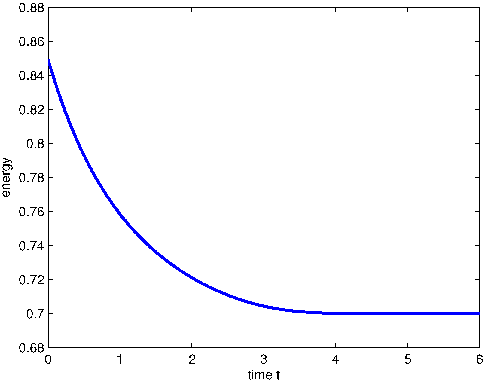
As clearly shown in Figure 2, the total energy decreases over time in Example 2 (1D) with $h=1/100$ and $\tau =1/1000$, which is in agreement with the theoretical energy decay property.

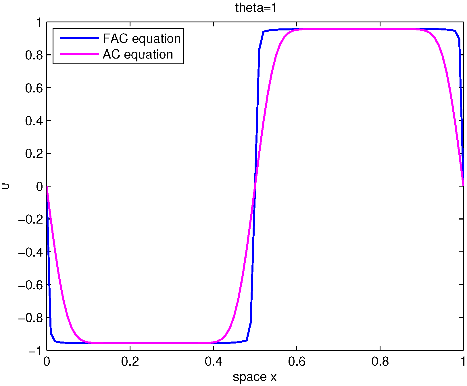
Figure 3 compares the equilibrium state of the FAC equation and AC equation in Example 2 (1D) at $t=5\mathrm{s}$ with $h=1/100$ and $\tau =1/1000$. It is evident that the interface width exhibited by the FAC equation is narrower than that of the AC equation with the same parameter values.

Figure 4 shows the comparison of different fractional orders $r=0.9$, $0.8$, and $0.7$ in Example 2 (1D) with $h=1/100$ and $\tau =1/1000$. The results indicate that as the fractional order r increases, the interface width becomes larger at the equilibrium state.

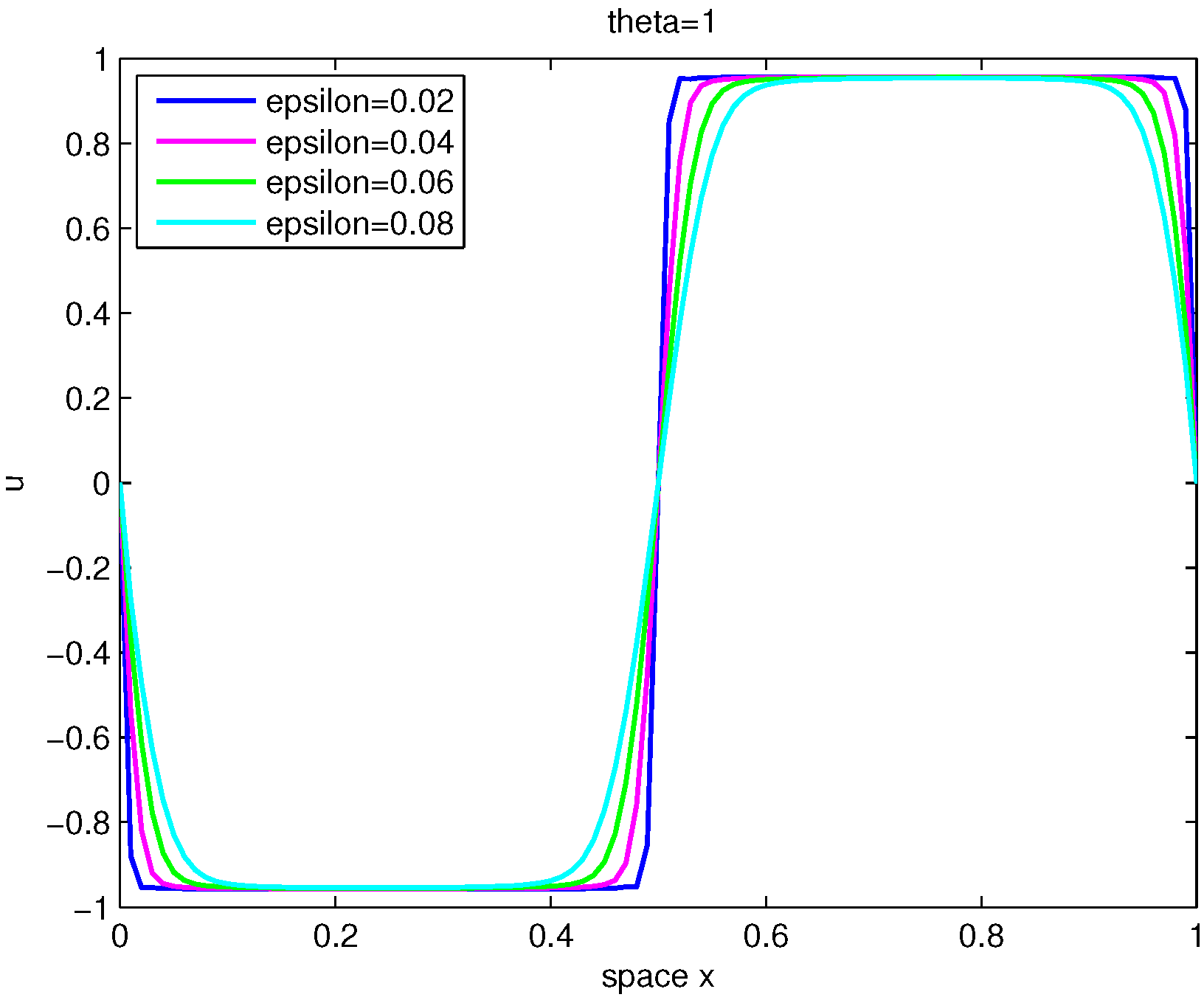
Figure 5 presents a comparison among different diffusion coefficients ($ϵ=0.02,$$0.04,$$0.06$, and $0.08$) in Example 2 (1D) with $h=1/100$ and $\tau =1/1000$. The results show that the interfacial width becomes broader as the coefficient $ϵ$ increases.

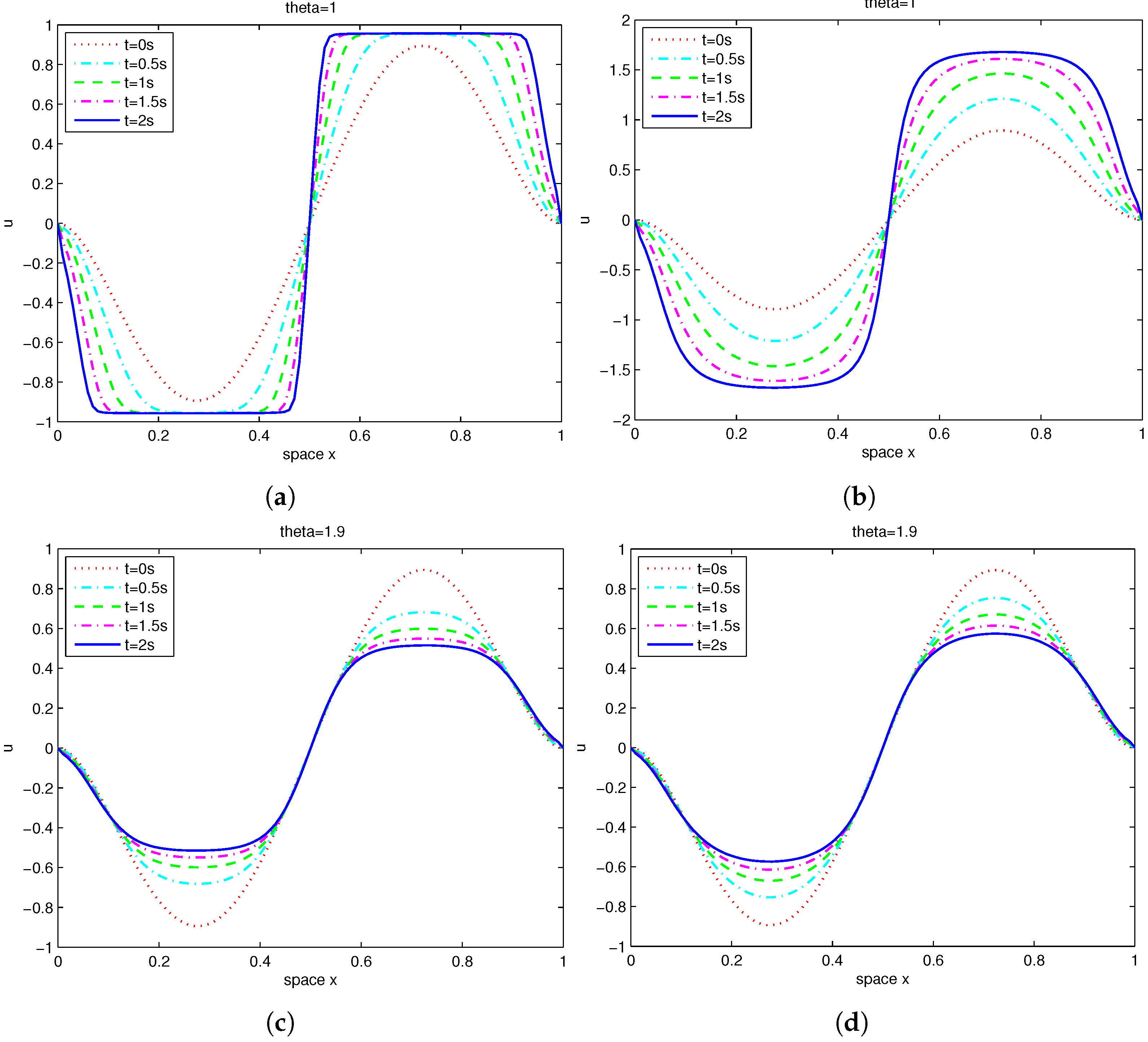
Figure 6 illustrates the phase separation process in FAC systems using a logarithmic potential (left) and a quartic polynomial potential (right) in Example 2 (1D) with $h=1/100$ and $\tau =1/1000$. The results demonstrate that as $\theta \to \omega$, the logarithmic potential can be approximated by a quartic polynomial. Furthermore, the comparison of Figure 6a,b reveals that systems governed by the logarithmic potential achieve better phase separation efficiency. This indicates that the logarithmic potential is not only a generalization of polynomial potentials; it plays a unique and indispensable role in computational modeling.

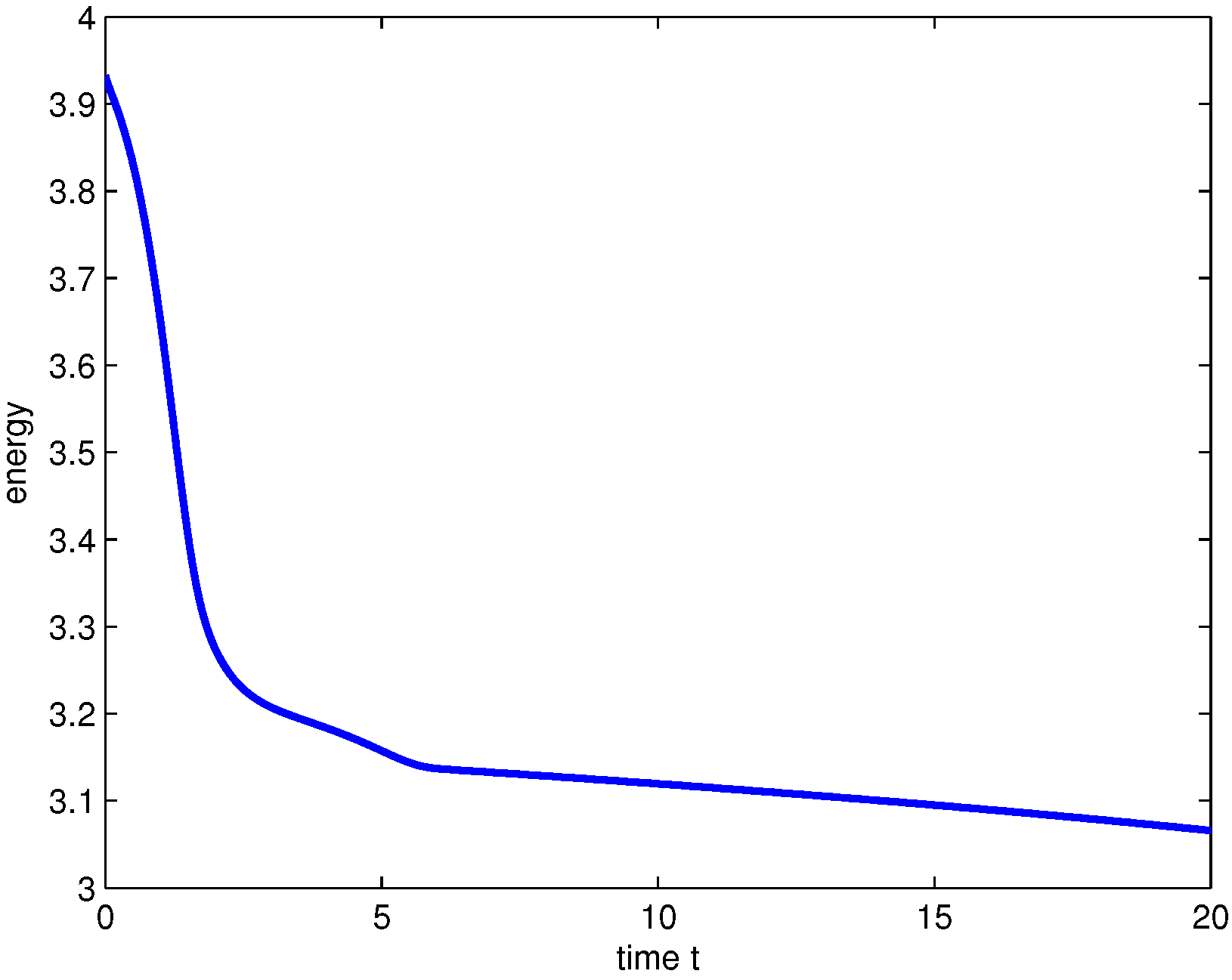
Example 3.

Take $r=0.8$, $\theta =1$, $\omega =2$, $\epsilon =0.1$, and $k=0.1$. Consider the following initial condition in Equation (43):

$$\begin{array}{c}\hfill u^0(x,y)=\left\{\begin{array}{cc}{\displaystyle \frac{1}{4}}tanh16d{r}_1,\hfill & \hfill -d{r}_1>d{r}_2,\\ -{\displaystyle \frac{1}{4}}tanh16d{r}_2,\hfill & \hfill -d{r}_1\le d{r}_2.\end{array}\right.\end{array}$$

(43)

Here, $\mathrm{\Omega }=[-1,1]\times [-1,1]$, $r_1=0.2$, $r_2=0.5$, $\mathbf{r}=\sqrt{x^2+y^2}$, $d{r}_1=\mathbf{r}-r_1$, and $d{r}_2=\mathbf{r}-r_2$. This initial condition simulates a radially symmetric phase-separated target pattern, with its core-shell structure corresponding to the initial state of spinodal decomposition commonly observed in binary mixtures after quenching.

Figure 7 shows the total energy of the coarsening processes in Example 3 (2D). The maximum diameter of the triangular elements is $h=0.0375$, and the time step is $\tau ={10}^{-3}$. It is obvious that the total energy is decreasing as time increases, which indicates that the finite element scheme obeys the physical property of the energy decay.

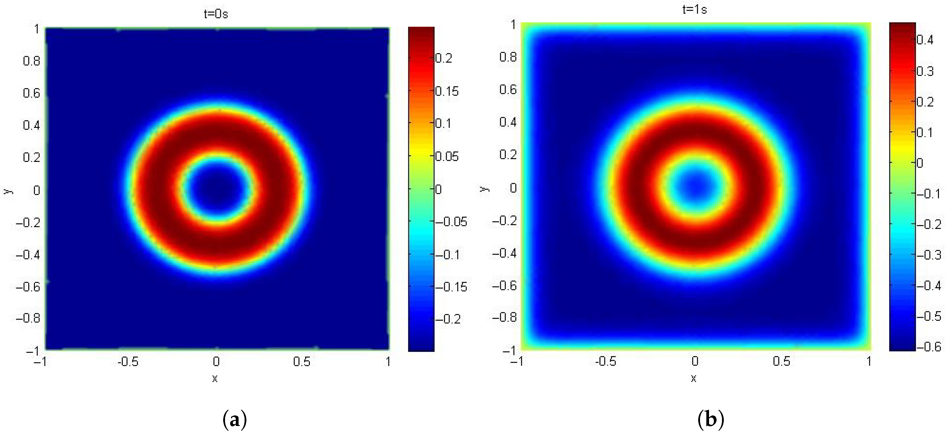
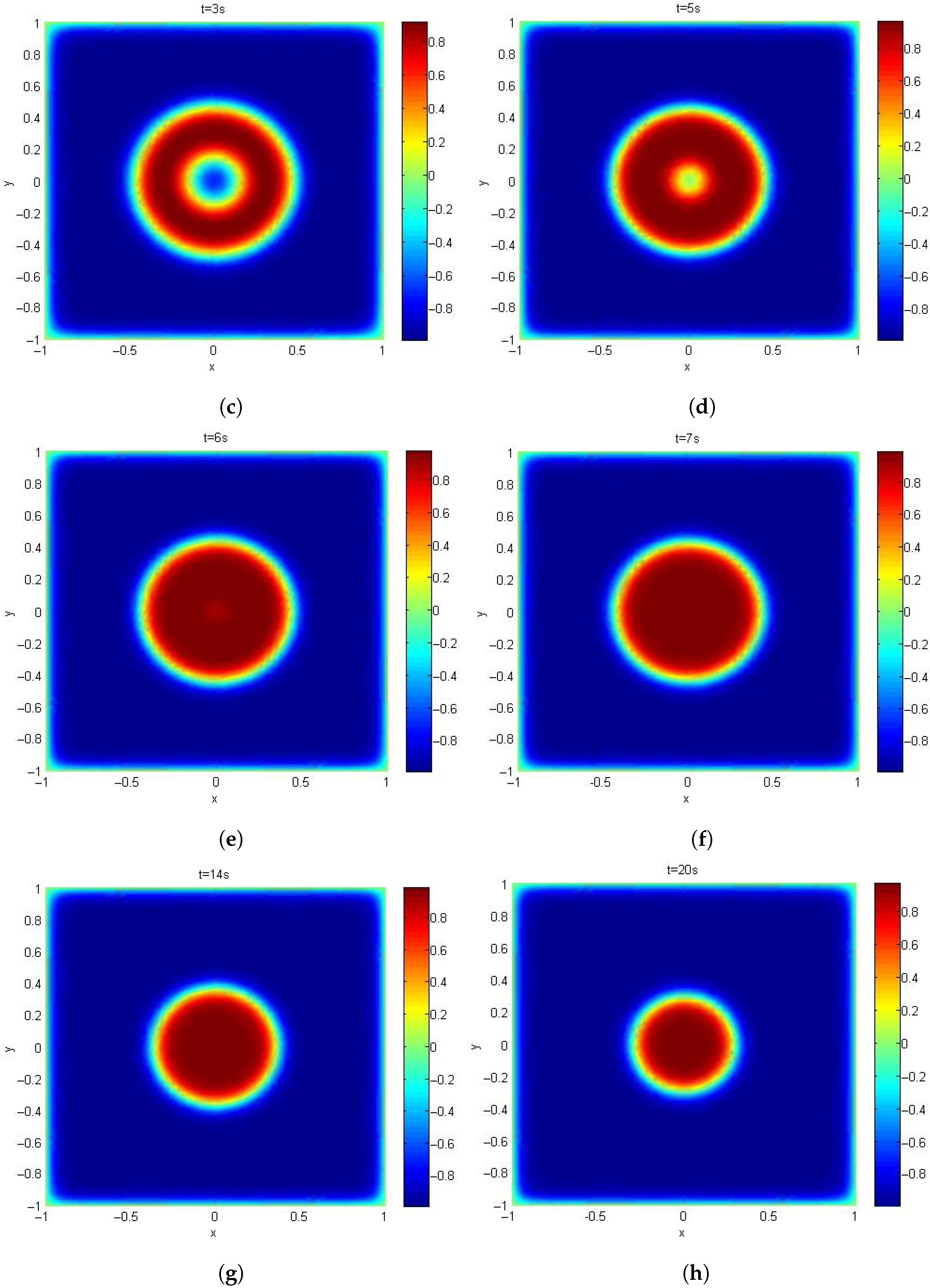
Figure 8 illustrates phase separation and interface coarsening phenomena in Example 3 (2D). The maximum diameter of the triangular elements is $h=0.0375$, and the time step is $\tau ={10}^{-3}$. The results show that, as time increases, the initially coexisting phases progressively separate into two pure phases, while the pure phase gradually coarsens. In this 2D case, the computation of $D_r$ refers to reference [26].

6. Conclusions

In this study, we develop a general framework for the ${\mathbb{R}}^d$ ($d=1,2,3$) fractional Allen–Cahn equation with a regularized logarithmic potential using k-th-order finite element space for spatial approximation and backward Euler scheme for temporal discretization. The existence and uniqueness of the discrete solution are established using the Brouwer fixed-point theorem, while the energy decay property and optimal convergence estimates are proven. Numerical experiments demonstrate that the regularized model (Equation (1)) may provide sharper interfaces and a more precise depiction of the coarsening process compared to both the classical Allen–Cahn equation and the double-well potential model.

While the dense matrix structure induced by the fractional Laplacian operator poses significant computational costs and storage challenges, efficient fast algorithms should be considered in future work, especially regarding comparisons of efficiency across different methods. Moreover, this numerical framework can be extended to the fractional Cahn–Hilliard equation with singular potentials, which is a meaningful research topic we are currently pursuing. Additionally, we will incorporate experimental parameters to conduct quantitative simulations of physical systems in subsequent work.