
Modeling and Neural Network Approximation of Asymptotic Behavior for Delta Fractional Difference Equations with Mittag-Leffler Kernels

 ,
,  ,
,  ,
,  and
and
Abstract
1. Introduction
2. Preliminaries
3. Asymptotic Behavior of -Order
- A sign condition and monotonicity result for whenever ;
- The asymptotic estimate of whenever .
4. Applications
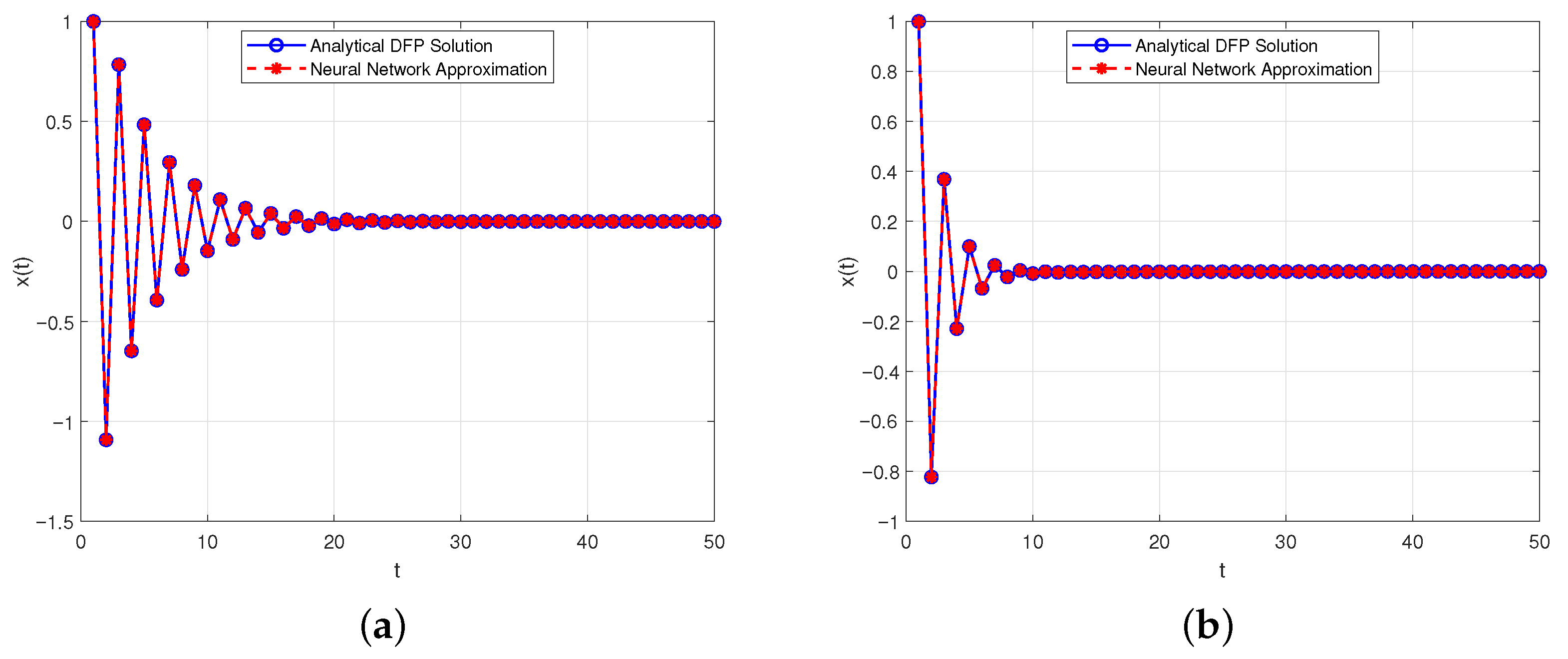
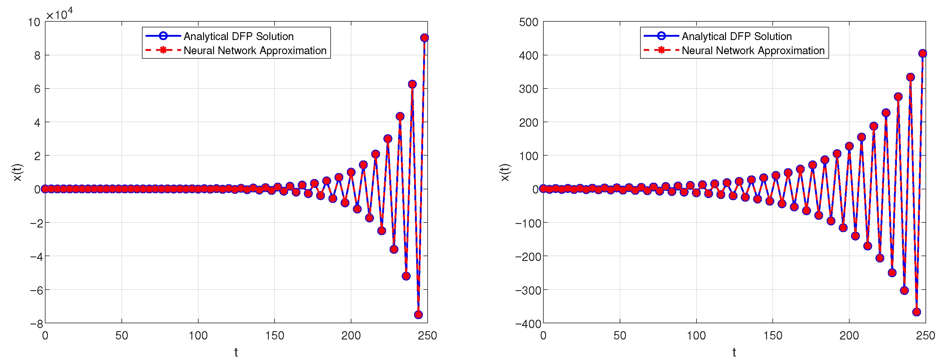
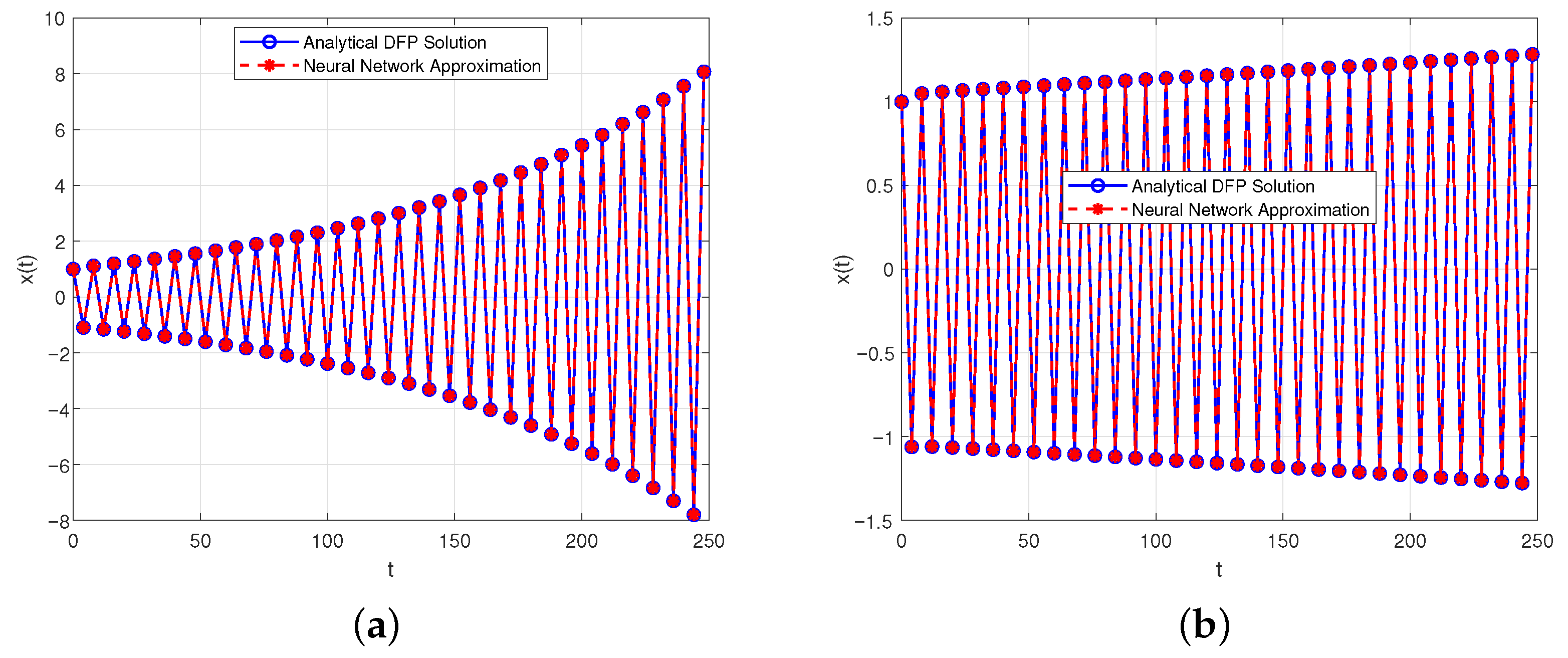
- Tends to 0 if ;
- Tends to ∞ if ;
- Is oscillatorily unstable if . That is,and
- is oscillatory stable if . That is,and
- Tends to 0 if .
4.1. Neural Network Approximation
- is oscillatorily stable for and ;
- is oscillatorily unstable for and ;
- will tend to 0 for and .

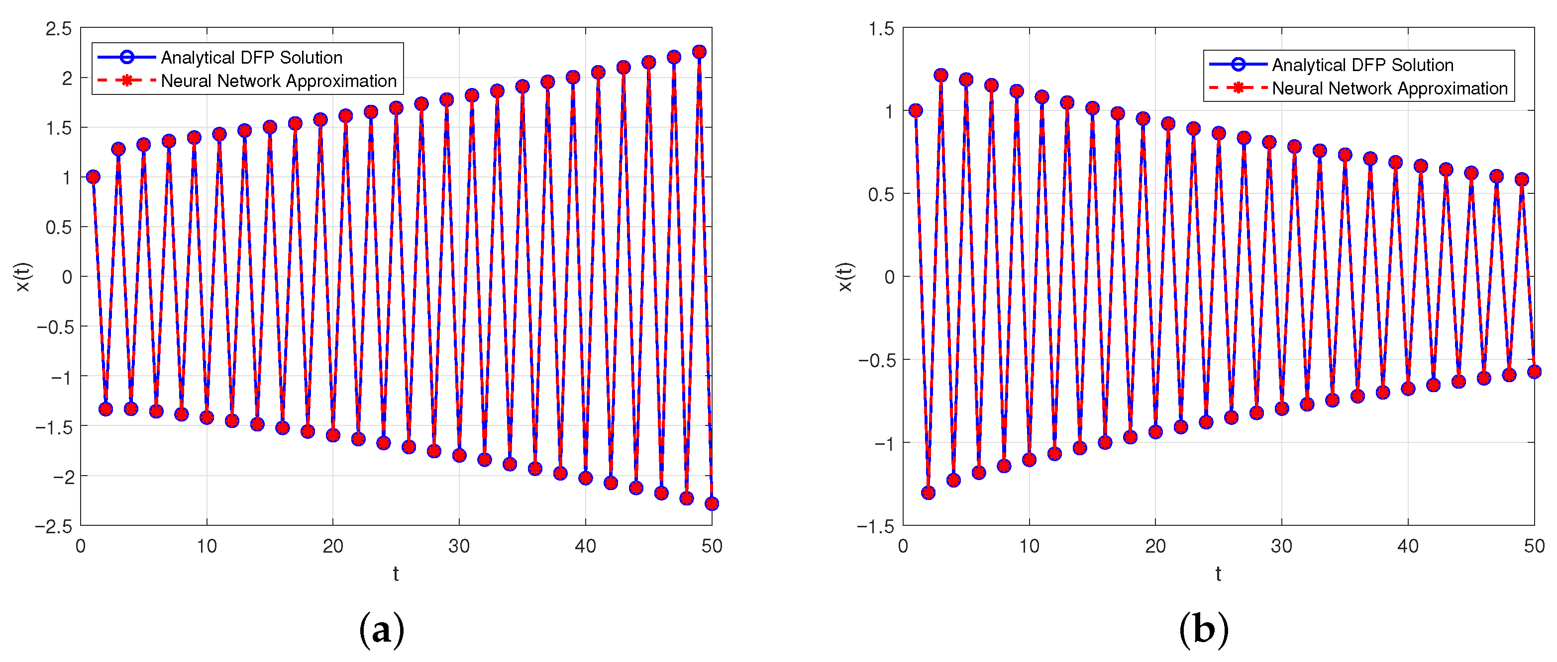
- is oscillatorily stable for and ;
- is oscillatorily unstable for and ;
- will tend to 0 for and .
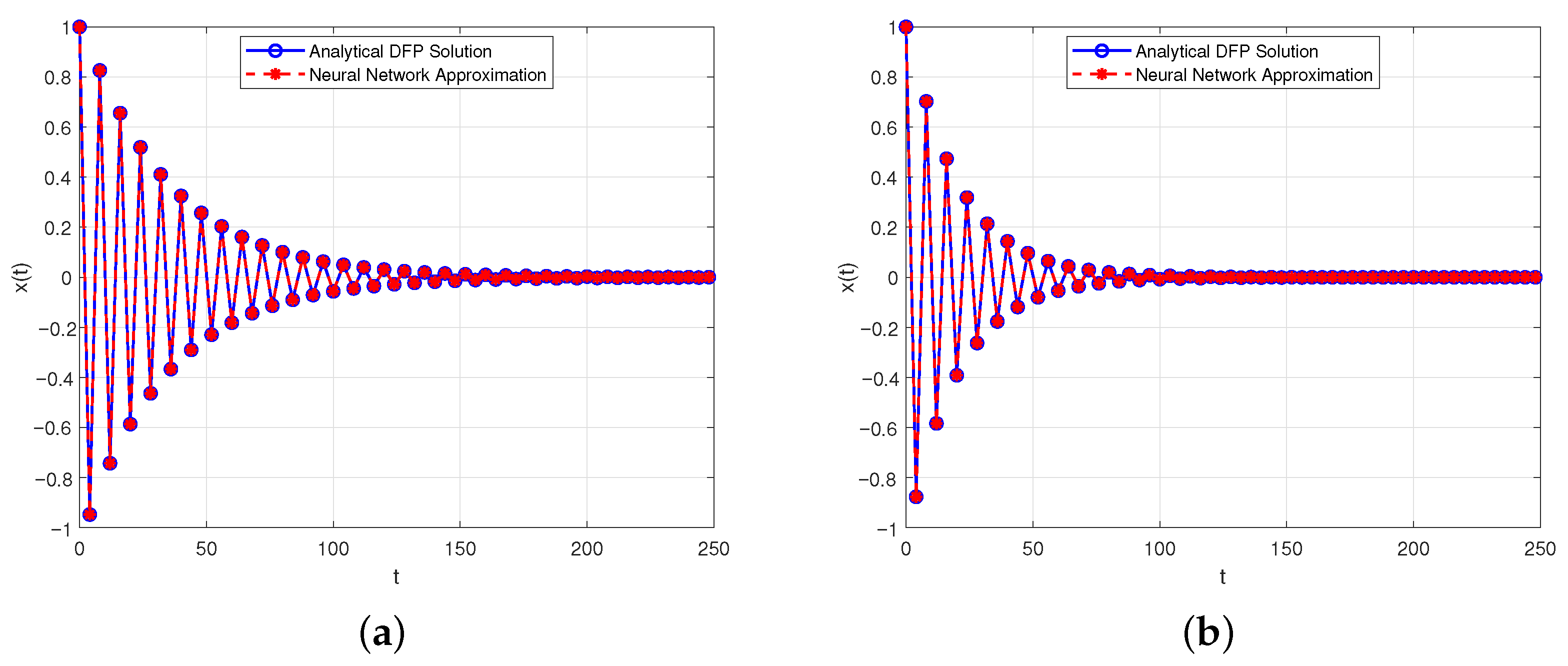
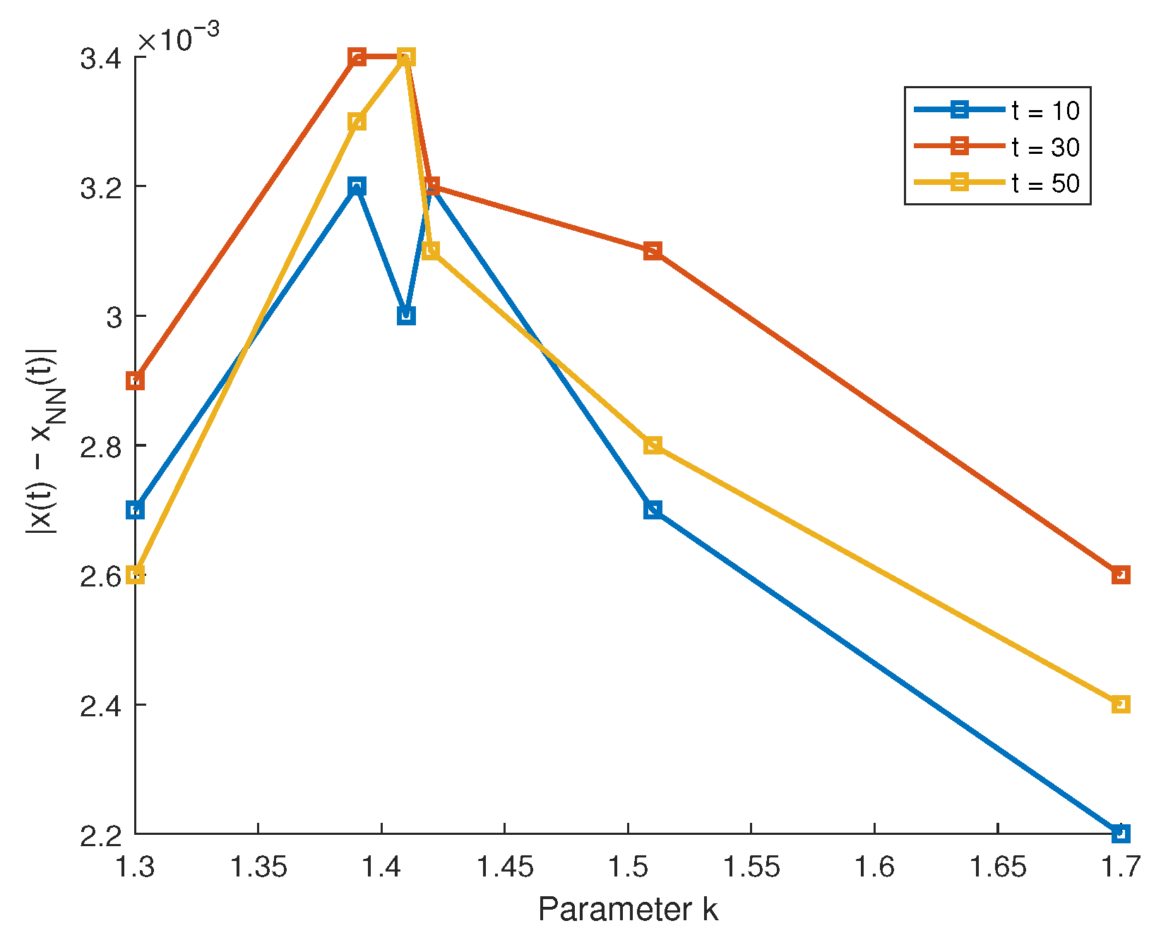
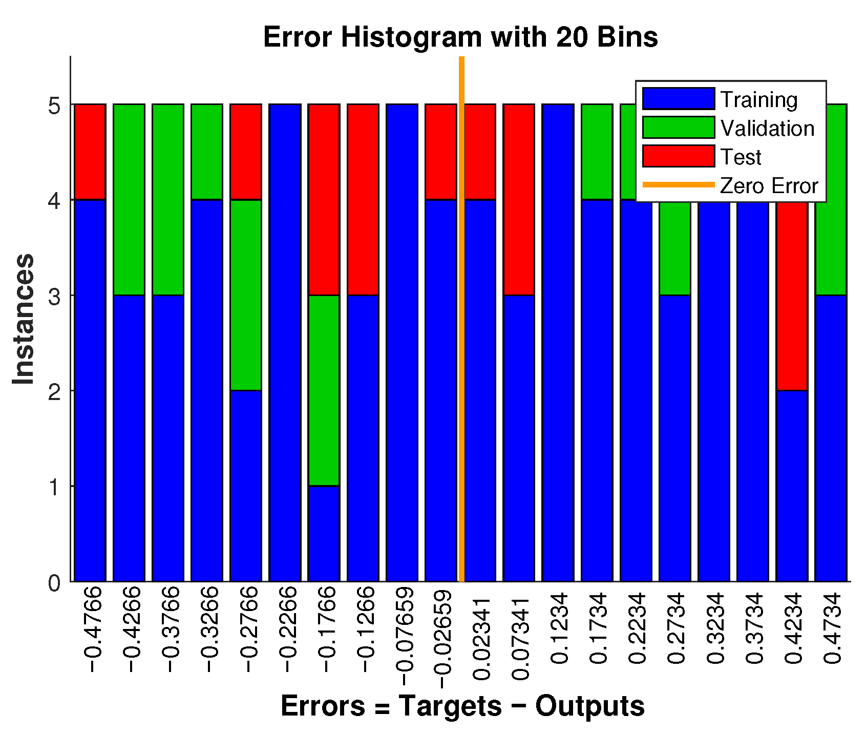
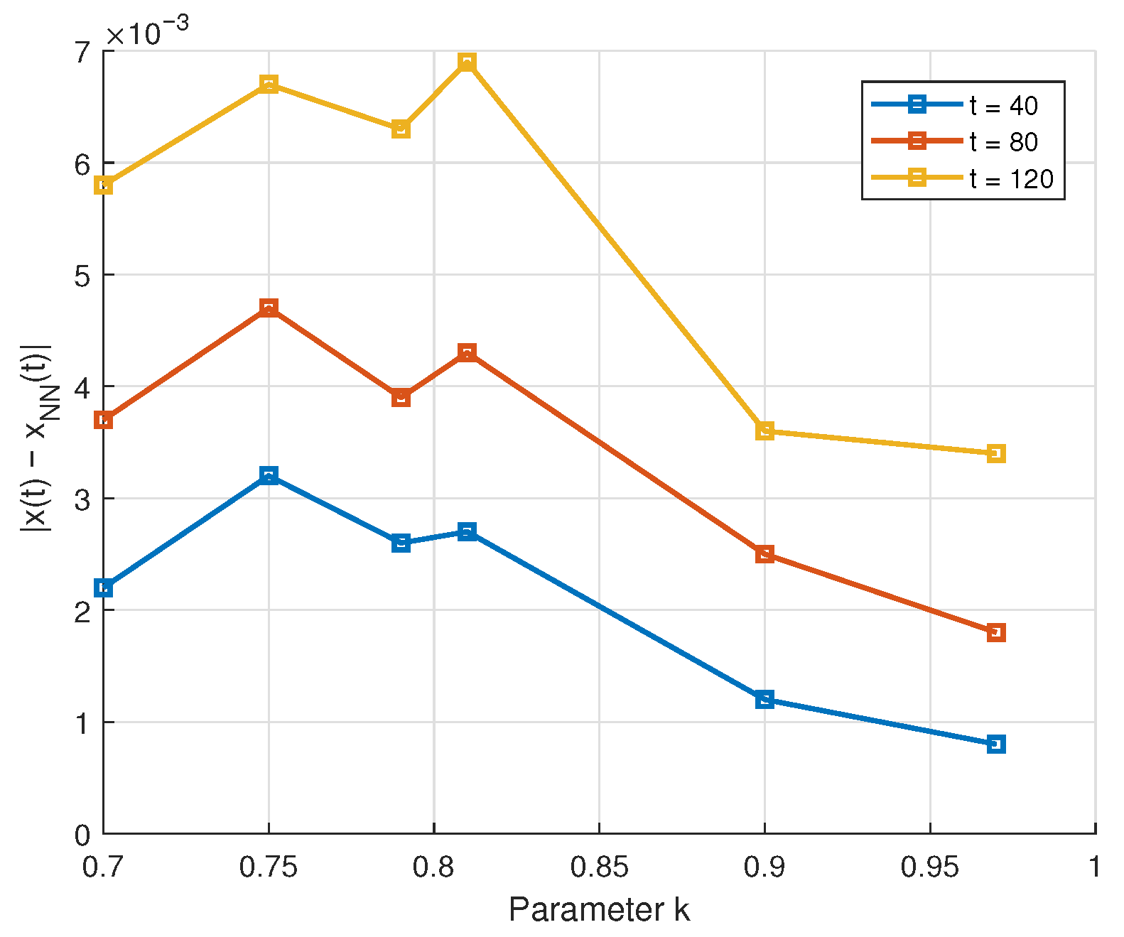
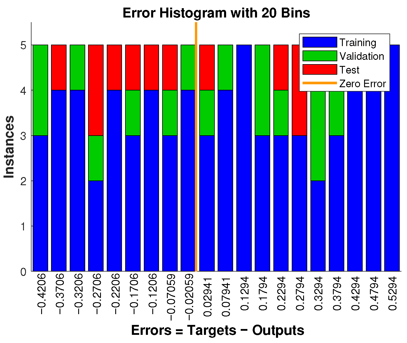
4.2. Algorithm for Solving the DFP and Neural Network Approximation
- Training ratio: 70%;
- Validation ratio: 15%;
- Testing ratio: 15%.
5. Conclusions and Future Direction
Author Contributions
Funding
Institutional Review Board Statement
Informed Consent Statement
Data Availability Statement
Acknowledgments
Conflicts of Interest
References
- Raubitzek, S.; Mallinger, K.; Neubauer, T. Combining Fractional Derivatives and Machine Learning: A Review. Entropy 2023, 25, 35. [Google Scholar] [CrossRef] [PubMed]
- Walasek, R.; Gajda, J. Fractional differentiation and its use in machine learning. Int. J. Adv. Eng. Sci. Appl. Math. 2021, 13, 270–277. [Google Scholar] [CrossRef]
- Chen, C. Discrete Caputo Delta Fractional Economic Cobweb Models. Qual. Theory Dyn. Syst. 2023, 22, 8. [Google Scholar] [CrossRef]
- Abdeljawad, T. Different type kernel h-fractional differences and their fractional h-sums. Chaos Solit. Fract. 2018, 116, 146–156. [Google Scholar] [CrossRef]
- Baleanu, D.; Wu, G.C. Some further results of the Laplace transform for variable-order fractional difference equations. Fract. Calc. Appl. Anal. 2019, 22, 1641–1654. [Google Scholar] [CrossRef]
- Dhawan, S.; Jonnalagadda, J.M. Nontrivial solutions for arbitrary order discrete relaxation equations with periodic boundary conditions. J. Anal. 2024, 32, 2113–2133. [Google Scholar] [CrossRef]
- Goodrich, C.S.; Peterson, A.C. Discrete Fractional Calculus; Springer: New York, NY, USA, 2015. [Google Scholar]
- Danca, M.-F.; Jonnalagadda, J.M. On the Solutions of a Class of Discrete PWC Systems Modeled with Caputo-Type Delta Fractional Difference Equations. Fractal Fract. 2023, 7, 304. [Google Scholar] [CrossRef]
- Guirao, J.L.G.; Mohammed, P.O.; Srivastava, H.M.; Baleanu, D.; Abualrub, M.S. A relationships between the discrete Riemann-Liouville and Liouville-Caputo fractional differences and their associated convexity results. AIMS Math. 2022, 7, 18127–18141. [Google Scholar] [CrossRef]
- Ikram, A. Lyapunov inequalities for nabla Caputo boundary value problems. J. Differ. Equ. Appl. 2018, 25, 757–775. [Google Scholar] [CrossRef]
- Atici, F.; Sengul, S. Modeling with discrete fractional equations. J. Math. Anal. Appl. 2010, 369, 1–9. [Google Scholar] [CrossRef]
- Silem, A.; Wu, H.; Zhang, D.-J. Discrete rogue waves and blow-up from solitons of a nonisospectral semi-discrete nonlinear Schrödinger equation. Appl. Math. Lett. 2021, 116, 107049. [Google Scholar] [CrossRef]
- Cabada, A.; Dimitrov, N. Nontrivial solutions of non-autonomous Dirichlet fractional discrete problems. Fract. Calc. Appl. Anal. 2020, 23, 980–995. [Google Scholar] [CrossRef]
- Mohammed, P.O.; Agarwal, R.P.; Yousif, M.A.; Al-Sarairah, E.; Lupas, A.A.; Abdelwahed, M. Theoretical Results on Positive Solutions in Delta Riemann-Liouville Setting. Mathematics 2024, 12, 2864. [Google Scholar] [CrossRef]
- Wang, P.; Liu, X.; Anderson, D.R. Fractional averaging theory for discrete fractional-order system with impulses. Chaos 2024, 34, 013128. [Google Scholar] [CrossRef] [PubMed]
- Eidelman, S.D.; Kochubei, A.N. Cauchy problem for fractional diffusion equations. J. Differ. Equ. 2004, 199, 211–255. [Google Scholar] [CrossRef]
- Karimova, E.; Ruzhansky, M.; Tokmagambetov, N. Cauchy type problems for fractional differential equations. Integral Transforms Spec. Funct. 2022, 33, 47–64. [Google Scholar] [CrossRef]
- Boutiara, A.; Rhaima, M.; Mchiri, L.; Makhlouf, A.B. Cauchy problem for fractional (p,q)-difference equations. AIMS Math. 2023, 8, 15773–15788. [Google Scholar] [CrossRef]
- Cinque, F.; Orsingher, E. Analysis of fractional Cauchy problems with some probabilistic applications. J. Math. Anal. Appl. 2024, 536, 128188. [Google Scholar] [CrossRef]
- Abdeljawad, T. Fractional difference operators with discrete generalized Mittag-Leffler kernels. Chaos Solit. Fract. 2019, 126, 315–324. [Google Scholar] [CrossRef]
- Mohammed, P.O.; Goodrich, C.S.; Hamasalh, F.K.; Kashuri, A.; Hamed, Y.S. On positivity and monotonicity analysis for discrete fractional operators with discrete Mittag-Leffler kernel. Math. Meth. Appl. Sci. 2022, 45, 6391–6410. [Google Scholar] [CrossRef]
- Nagai, A. Discrete Mittag–Leffler function and its applications. Publ. Res. Inst. Math. Sci. Kyoto Univ. 2003, 1302, 1–20. [Google Scholar]
- Awadalla, M.; Mahmudov, N.I.; Alahmadi, J. A novel delayed discrete fractional Mittag-Leffler function: Representation and stability of delayed fractional difference system. J. Appl. Math. Comput. 2024, 70, 1571–1599. [Google Scholar] [CrossRef]
- Saenko, V.V. The calculation of the Mittag–Leffler function. Int. J. Comput. Math. 2022, 99, 1367–1394. [Google Scholar] [CrossRef]
- Wu, G.C.; Baleanu, D.; Zeng, S.D.; Luo, W.H. Mittag–Leffler function for discrete fractional modelling. J. King Saud Univ. Sci. 2016, 28, 99–102. [Google Scholar] [CrossRef]
- Mohammed, P.O.; Abdeljawad, T.; Hamasalh, F.K. Discrete Prabhakar fractional difference and sum operators. Chaos Solit. Fractals 2021, 150, 111182. [Google Scholar] [CrossRef]
- Abdeljawad, T.; Baleanu, D. Discrete fractional differences with nonsingular discrete Mittag-Leffler kernels. Adv. Differ. Equ. 2016, 232, 2016. [Google Scholar]
- Wei, Y.; Zhao, L.; Lu, J.; Cao, J. Stability and Stabilization for Delay Delta Fractional Order Systems: An LMI Approach. IEEE Trans. Circuits Syst. II: Express Br. 2023, 70, 4093–4097. [Google Scholar] [CrossRef]
- Jonnalagadda, J.M. A Comparison Result for the Nabla Fractional Difference Operator. Foundations 2023, 3, 181–198. [Google Scholar] [CrossRef]
- Mohammed, P.O.; Lizama, C.; Lupas, A.A.; Al-Sarairah, E.; Abdelwahed, M. Maximum and Minimum Results for the Green’s Functions in Delta Fractional Difference Settings. Symmetry 2024, 16, 991. [Google Scholar] [CrossRef]
- Gholami, Y. A uniqueness criterion for nontrivial solutions of the nonlinear higher-order ∇-difference systems of fractional-order. Fract. Differ. Calc. 2021, 11, 85–110. [Google Scholar] [CrossRef]
- Goodrich, C.S. A comparison result for the fractional difference operator. Int. J. Differ. Equ. 2011, 6, 17–37. [Google Scholar]
- Jia, B.; Du, F.; Erbe, L.; Peterson, A. Asymptotic behavior of nabla half order h-difference equations. JAAC 2018, 8, 1707–1726. [Google Scholar]
- Du, F.; Lu, J.-G. Explicit solutions and asymptotic behaviors of Caputo discrete fractional-order equations with variable coefficients. Chaos Solit. Fractals 2021, 153, 111490. [Google Scholar] [CrossRef]
- Jia, B.; Lynn, E.; Peterson, A. Comparison theorems and asymptotic behavior of solutions of discrete fractional equations. Electron. J. Qual. Theory Differ. Equ. 2015, 89, 1–18. [Google Scholar] [CrossRef]
- Jonnalagadda, J.M. Asymptotic behaviour of linear fractional nabla difference equations. Int. J. Differ. Equ. 2017, 12, 255–265. [Google Scholar]
- Wang, M.; Jia, B.; Du, F.; Liu, X. Asymptotic stability of fractional difference equations with bounded time delays. Fract. Calc. Appl. Anal. 2020, 23, 571–590. [Google Scholar] [CrossRef]
- Brackins, A. Boundary Value Problems of Nabla Fractional Difference Equations. Ph.D.Thesis, The University of Nebraska, Lincoln, NE, USA, 2014. [Google Scholar]
- Chen, C.; Bohner, M.; Jia, B. Existence and uniqueness of solutions for nonlinear Caputo fractional difference equations. Turk. J. Math. 2020, 44, 857–869. [Google Scholar] [CrossRef]
- Mohammed, P.O. On Asymptotic Behavior Solutions for Delta Fractional Differences. Commun. Nonlinear Sci. Numer. Simul.
- Muresan, M. A Concrete Approach to Classical Analysis; Springer: Berlin/Heidelberg, Germany, 2009. [Google Scholar]
- Dutka, J. The early history of the factorial function. Arch. Hist. Exact Sci. 1991, 43, 225–249. [Google Scholar] [CrossRef]
- Javadi, R.; Mesgarani, H.; Nikan, O.; Avazzadeh, Z. Solving Fractional Order Differential Equations by Using Fractional Radial Basis Function Neural Network. Symmetry 2023, 15, 1275. [Google Scholar] [CrossRef]
- Sivalingam, S.M.; Kumar, P.; Govindaraj, V. A Neural Networks-Based Numerical Method for the Generalized Caputo-Type Fractional Differential Equations. Math. Comput. Simul. 2023, 213, 302–323. [Google Scholar]
- Allahviranloo, T.; Jafarian, A.; Saneifard, R.; Ghalami, N.; Measoomy Nia, S.; Kiani, F.; Fernandez-Gamiz, U.; Noeiaghdam, S. An Application of Artificial Neural Networks for Solving Fractional Higher-Order Linear Integro-Differential Equations. Bound. Value Probl. 2023, 2023, 74. [Google Scholar] [CrossRef]
- Mohammed, P.O.; Kürt, C.; Abdeljawad, T. Bivariate discrete Mittag-Leffler functions with associated discrete fractional operators. Chaos Solit. Fractals 2022, 165, 112848. [Google Scholar] [CrossRef]
- Mohammed, P.O.; Abdeljawad, T. Discrete generalized fractional operators defined using h-discrete Mittag-Leffler kernels and applications to AB fractional difference systems. Math. Meth. Appl. Sci. 2020, 46, 7688–7713. [Google Scholar] [CrossRef]

| k | t | Present Work | NN Approx. | Absolute Error |
|---|---|---|---|---|
| 1.30 | 10 | 0.8432 | 0.8405 | 0.0027 |
| 30 | 0.9207 | 0.9178 | 0.0029 | |
| 50 | 0.9815 | 0.9789 | 0.0026 | |
| 1.39 | 10 | 0.7634 | 0.7602 | 0.0032 |
| 30 | 0.8159 | 0.8125 | 0.0034 | |
| 50 | 0.8650 | 0.8617 | 0.0033 | |
| 1.41 | 10 | 0.7210 | 0.7180 | 0.0030 |
| 30 | 0.7642 | 0.7608 | 0.0034 | |
| 50 | 0.8005 | 0.7971 | 0.0034 | |
| 1.42 | 10 | 0.6905 | 0.6873 | 0.0032 |
| 30 | 0.7321 | 0.7289 | 0.0032 | |
| 50 | 0.7659 | 0.7628 | 0.0031 | |
| 1.51 | 10 | 0.5387 | 0.5360 | 0.0027 |
| 30 | 0.5735 | 0.5704 | 0.0031 | |
| 50 | 0.6023 | 0.5995 | 0.0028 | |
| 1.70 | 10 | 0.3251 | 0.3229 | 0.0022 |
| 30 | 0.3467 | 0.3441 | 0.0026 | |
| 50 | 0.3649 | 0.3625 | 0.0024 |
| k | Absolute Error | |
|---|---|---|
| 0.25 | 0.0013 | |
| 1.39 | 0.50 | 0.0021 |
| 0.75 | 0.0034 | |
| 0.25 | 0.0011 | |
| 1.42 | 0.50 | 0.0018 |
| 0.75 | 0.0030 | |
| 0.25 | 0.0007 | |
| 1.70 | 0.50 | 0.0013 |
| 0.75 | 0.0023 |
| k | Mean Absolute Error (MAE) |
|---|---|
| 1.30 | 0.0040 |
| 1.39 | 0.0045 |
| 1.41 | 0.0052 |
| 1.42 | 0.0055 |
| 1.51 | 0.0061 |
| 1.70 | 0.0065 |
| k | t | Present Work | NN Approx. | Absolute Error |
|---|---|---|---|---|
| 0.70 | 40 | 1.1814 | 1.1792 | 0.0022 |
| 80 | 1.3567 | 1.3530 | 0.0037 | |
| 120 | 1.5563 | 1.5505 | 0.0058 | |
| 0.75 | 40 | 1.2045 | 1.2013 | 0.0032 |
| 80 | 1.4018 | 1.3971 | 0.0047 | |
| 120 | 1.6279 | 1.6212 | 0.0067 | |
| 0.79 | 40 | 1.2236 | 1.2210 | 0.0026 |
| 80 | 1.4382 | 1.4343 | 0.0039 | |
| 120 | 1.6804 | 1.6741 | 0.0063 | |
| 0.81 | 40 | 1.2319 | 1.2292 | 0.0027 |
| 80 | 1.4537 | 1.4494 | 0.0043 | |
| 120 | 1.7052 | 1.6983 | 0.0069 | |
| 0.90 | 40 | 0.9251 | 0.9263 | 0.0012 |
| 80 | 0.8577 | 0.8602 | 0.0025 | |
| 120 | 0.7954 | 0.7990 | 0.0036 | |
| 0.97 | 40 | 0.8903 | 0.8895 | 0.0008 |
| 80 | 0.8109 | 0.8127 | 0.0018 | |
| 120 | 0.7381 | 0.7415 | 0.0034 |
| k | Absolute Error | |
|---|---|---|
| 0.25 | 0.0028 | |
| 0.75 | 0.50 | 0.0032 |
| 0.75 | 0.0039 | |
| 0.25 | 0.0024 | |
| 0.81 | 0.50 | 0.0027 |
| 0.75 | 0.0034 | |
| 0.25 | 0.0019 | |
| 0.97 | 0.50 | 0.0021 |
| 0.75 | 0.0028 |
| k | Mean Absolute Error (MAE) |
|---|---|
| 1.30 | 0.0040 |
| 1.39 | 0.0045 |
| 1.41 | 0.0052 |
| 1.42 | 0.0055 |
| 1.51 | 0.0061 |
| 1.70 | 0.0065 |
Disclaimer/Publisher’s Note: The statements, opinions and data contained in all publications are solely those of the individual author(s) and contributor(s) and not of MDPI and/or the editor(s). MDPI and/or the editor(s) disclaim responsibility for any injury to people or property resulting from any ideas, methods, instructions or products referred to in the content. |
© 2025 by the authors. Licensee MDPI, Basel, Switzerland. This article is an open access article distributed under the terms and conditions of the Creative Commons Attribution (CC BY) license (https://creativecommons.org/licenses/by/4.0/).
Share and Cite
Mohammed, P.O.; Alharthi, M.R.; Yousif, M.A.; Lupas, A.A.; Azzo, S.M. Modeling and Neural Network Approximation of Asymptotic Behavior for Delta Fractional Difference Equations with Mittag-Leffler Kernels. Fractal Fract. 2025, 9, 452. https://doi.org/10.3390/fractalfract9070452
Mohammed PO, Alharthi MR, Yousif MA, Lupas AA, Azzo SM. Modeling and Neural Network Approximation of Asymptotic Behavior for Delta Fractional Difference Equations with Mittag-Leffler Kernels. Fractal and Fractional. 2025; 9(7):452. https://doi.org/10.3390/fractalfract9070452
Chicago/Turabian StyleMohammed, Pshtiwan Othman, Muteb R. Alharthi, Majeed Ahmad Yousif, Alina Alb Lupas, and Shrooq Mohammed Azzo. 2025. "Modeling and Neural Network Approximation of Asymptotic Behavior for Delta Fractional Difference Equations with Mittag-Leffler Kernels" Fractal and Fractional 9, no. 7: 452. https://doi.org/10.3390/fractalfract9070452
APA StyleMohammed, P. O., Alharthi, M. R., Yousif, M. A., Lupas, A. A., & Azzo, S. M. (2025). Modeling and Neural Network Approximation of Asymptotic Behavior for Delta Fractional Difference Equations with Mittag-Leffler Kernels. Fractal and Fractional, 9(7), 452. https://doi.org/10.3390/fractalfract9070452