1. Introduction
The study of time-fractional Navier–Stokes equations (TFNSEs) has emerged as a pivotal area in modern applied mathematics, offering a powerful framework for modeling complex fluid dynamics with memory and hereditary properties [
1,
2,
3,
4,
5,
6]. Unlike their integer-order counterparts, these equations employ Caputo fractional derivatives to capture non-local temporal dependencies, making them particularly suitable for describing anomalous diffusion in viscoelastic fluids, turbulent flows, and fractal porous media [
4,
7,
8,
9]. The fractional derivative operator
(where
) introduces a convolution kernel that captures the entire history of the system. This memory effect enables more accurate modeling of frequency-dependent damping and power-law relaxation phenomena. Such characteristics are frequently observed in various real-world applications [
8,
10].
From a physical perspective, the nonlinear damping term
(with
) plays several pivotal roles in fluid dynamics modeling [
11]. Most notably, it strengthens the system’s energy dissipation mechanisms, which are essential for accurately capturing the rapid energy decay characteristic of turbulent flows and porous media systems [
12,
13]. In addition to enhancing dissipation, this term contributes critical stabilization by preventing finite-time blow-up in high-Reynolds-number regimes, where classical Navier–Stokes formulations often fail [
14].
The damping term’s physical significance extends to daily-life applications, including biological flows like blood circulation, where it models shear-dependent vascular resistance, and geophysical flows such as ocean dynamics, where it accounts for small-scale turbulence dissipation [
9]. These practical applications are supported by systematic mathematical foundations. Theoretical studies have demonstrated that the presence of
ensures three key properties: first, the global existence of weak solutions for
without dimensional restrictions; second, enhanced solution regularity when
in
d-dimensional domains; and third, suppression of energy accumulation at high frequencies, effectively serving as a natural turbulence regularization mechanism [
14,
15,
16].
The numerical solutions of TFNSEs present significant challenges due to their inherent mathematical complexity [
15,
17,
18]. Key difficulties arise from the non-local nature of Caputo derivatives, which requires the entire solution history to be processed and stored, thus leading to increased computational costs [
19]. Moreover, the nonlinear interaction between the fractional temporal operator, the convective term
, and the damping effects complicates stability analysis and convergence proofs [
15]. Although its mathematical structure and physical implications with hybrid methods have been discussed in prior studies [
11,
13,
14,
20], the development of numerical methods that specifically address an L1-type scheme with a nonlinear damping term has still not been covered in the existing literature within the finite element method.
To find the solution of these complex models (TFNSEs) with nonlinear damping, we propose a hybrid-type fully discrete scheme using mixed finite element spaces – and – combined with an L1-type scheme. This approach ensures both stability and accuracy in approximating velocity and pressure variables. We establish optimal error estimates in the -norm for velocity and -norm for pressure, carefully accounting for the interaction between fractional memory and nonlinear damping.
The unconditional stability of both semi-discrete and fully discrete schemes is theoretically demonstrated and corroborated through comprehensive numerical experiments. We implement four distinct algorithms and validate them across three representative test cases. The first test assesses the accuracy of the mixed finite element pairs for various fractional orders
and damping exponents
r. The second verifies convergence behavior using exact solutions under similar parameter variations, while the third focuses on the nonlinear damping effects utilizing Algorithms 1–4. Furthermore, the scheme is applied to two classical benchmark flows, the backward-facing step [
21], showcasing flow separation and reattachment, and the lid-driven cavity [
22], characterized by complex vortex structures, to demonstrate its capability in capturing both internal and external flow dynamics. This work makes three key contributions to the scientific community, detailed as follows.
First, we develop a novel hybrid numerical scheme combining finite difference methods (for L1 time discretization of Caputo derivatives with ) with mixed finite elements (Taylor–Hood - and mini - elements for velocity–pressure approximation). Second, we establish rigorous stability analysis and prove optimal convergence rates of for velocity and for pressure, which are verified numerically. Third, this represents the first complete finite element framework capable of handling the full complexity of time-fractional Navier–Stokes equations with nonlinear damping , successfully addressing the coupled challenges of (a) fractional temporal operators, (b) nonlinear convection, and (c) power-law damping. The method’s effectiveness is demonstrated through comprehensive benchmark tests of turbulent flows with memory effects (back channel flow and cavity flow).
Extensive numerical results, validated against exact solutions, indicate that our method achieves comparable or superior accuracy relative to existing approaches [
16,
23], while significantly improving computational efficiency, especially across a range of fractional parameters
and damping exponents
r. These findings underscore the robustness and effectiveness of the proposed scheme for simulating complex fluid behaviors governed by fractional dynamics with nonlinear damping.
This work is organised as follows.
Section 2 establishes the time-fractional Navier–Stokes equations with nonlinear damping, where the fractional derivative is considered in the Caputo sense for
.
Section 3 develops the numerical framework, combining mixed finite elements for spatial discretization with an L1 scheme for the temporal fractional derivative.
Section 4 provides the finite difference method, stability analysis, and derives optimal order error estimates for semi–discrete and fully discrete formulations. Numerical experiments in
Section 5 illustrate the scheme’s performance on well–known algorithms and verify theoretical convergence rates with different given true solutions by Mini elements
–
and Taylor–Hood
–
elements. The work concludes in
Section 6 with a conclusion paragraph and some future work related to complex flow models.
| Algorithm 1 Linearization using previous iterations for both nonlinear terms. |
Set initial guesses , . For , find such that for all , If , accept the solution. Otherwise, set and repeat Step II.
|
| Algorithm 2 Update damping term using current iteration |
|
| Algorithm 3 Update convective term using current iteration |
|
| Algorithm 4 Fully updated nonlinear iteration |
|
3. Notations, Preliminaries and Mixed Weak Formulation
In this section, we introduce notations and preliminary concepts related to functional spaces. We begin with the following standard Hilbert spaces [
22,
25,
26]:
where
is equipped with the classical inner product
and corresponding norm
. The space
is endowed with the inner product and norm:
Let
and
represent the divergence-free subspaces defined by
We define the Stokes operator
by
where
denotes the standard Laplacian applied component-wise, and
is the
-orthogonal Helmholtz–Leray projection from the space
onto the subspace
of divergence-free vector fields with a vanishing normal trace on the boundary
. This projection ensures compatibility with the incompressibility condition
and arises naturally in the variational formulation of the Stokes and Navier–Stokes equations [
27,
28].
The domain of
is defined as
where
. This guarantees that the Laplacian
is well defined in a weak sense and respects both the divergence-free condition and the Dirichlet boundary condition. The space
ensures sufficient regularity, while the intersection with
enforces incompressibility.
To define intermediate regularity spaces, we introduce the fractional powers of the Stokes operator. For a dummy variable
, we define
with the norm
, which is equivalent to standard Sobolev norms on divergence-free spaces [
29]. This leads to a scale of Hilbert spaces:
This framework is essential in analyzing the regularity, stability, and long-term behavior of solutions to the Navier–Stokes equations. The spectral theory of the Stokes operator and the associated fractional power spaces are crucial for establishing energy estimates and proving the existence and uniqueness of both weak and strong solutions [
28,
29].
Following [
30], we define the Riemann–Liouville fractional integral operator of order
, which generalizes the classical integral to fractional orders, as
where
is the gamma function defined by
A is a dummy variable for integration, and we adopt the convention when the order is zero, recovering the original function.
The Caputo-type derivative
, which appears in Equation (1), is a widely used fractional derivative formulation, particularly suitable for initial value problems, as it naturally incorporates initial conditions. For order
, it is defined by
where the derivative is applied after subtracting the initial value, ensuring consistency with the classical derivative when
.
Moreover, as described in [
31], the
fractional integral operator , which acts as the inverse of the Caputo derivative and generalizes repeated integration to fractional orders, is given by
Next, we define the following continuous bilinear and trilinear forms that will be used throughout the analysis. Specifically, we introduce the bilinear forms
on
,
on
, and the trilinear forms
and
on
, defined, respectively, as
and
It is well known (see [
32,
33]) that the trilinear form
satisfies the following properties:
and the boundedness estimate
where
denotes the
-norm, and
is a positive constant.
Theorem 1 ([
29,
34])
. There exists at least a solution pair to satisfywhere 3.1. Variational Formulation
Based on the above notations, we formulate the weak formulation of the model (
1) as follows. Find
and
such that for all test functions
and
, the following equations hold:
For the short and concise representation, Equation (
7) can be written as
In [
15], Zhou and Peng established the existence and uniqueness of weak solutions for problem (
8) in the case without the time-fractional term. However, the uniqueness of weak solutions and the global (in time) existence of strong solutions remain completely open questions.
3.2. Uniqueness
We will prove that the strong solution is unique in the larger class of weak solutions for any . More precisely, we provide a theorem.
Theorem 2 ([
24])
. Assume and are two solutions to (1) with the same initial condition . Then on . Proof. Let
w denote the difference between the two solutions, i.e.,
. By linearity,
w satisfies the following equation obtained by subtracting the weak formulations for
and
:
with
and
.
Taking the
inner product of (
9) with
w and integrating by parts yields the following:
The damping term is non-negative due to the monotonicity of
:
From (
10), we deduce
where we used Hölder’s inequality, the 2D Gagliardo-Nirenberg inequality
(see the references for more utilizations [
26,
35]), and Young’s inequality.
Simplifying and applying Grönwall’s inequality [
31,
36] gives the following:
since
and
. Thus,
on
, the proof is completed. □
4. Spatially Discrete Finite Element Formulation
Let
be a shape-regular triangulation of the reference domain
, where each element
K is a closed simplex with diameter
[
37]. We define the local mesh size function
piecewise as
for all
and the global mesh parameter as
, representing the largest element diameter in the triangulation [
38]. The shape regularity condition requires the existence of a constant
such that
for all
, where
denotes the radius of element
K ([
39] [Section 3.1]).
We consider a mixed finite element approximation space , where
is the discrete velocity space;
is the discrete pressure space. The corresponding divergence-free subspace
is defined by
where
represents the bilinear form of divergence.
Let
denote the
-orthogonal projection operator, uniquely determined by
The following fundamental assumptions on the mixed finite element spaces will be essential for our analysis [
32,
40].
Assumption 1 ([
34,
39])
. Approximation Property: For any , there exist approximations , and a positive constant independent of the mesh size h, such that Assumption 2 ([
41,
42])
. For any , the following relations hold: Assumption 3 ([
34,
39,
42])
. For all , there exists , such that Assumption 4 ([
39])
. The -projection operator satisfies the following approximation properties:- 1.
For all , the Stokes operator domain is - 2.
The semi-discrete FEM seeks
, satisfying
with
. The discrete Stokes operator
satisfies
. The trilinear form
is anti-symmetric, conservative (
), and bounded [
27].
Lemma 1 (Caputo Inequality)
. Let and . Then, the Caputo fractional derivative satisfies the coercivity identitywhere denotes the Caputo fractional derivative of order α. Theorem 3 (Uniqueness and Stability)
. Let () be the semi-discrete finite element approximation of the solution of the TFNS problem with nonlinear damping. Then, for any , the following estimate holds:where and . Proof. Choosing test functions
in Equation (
18), we can obtain the following:
We begin with the weak formulation tested by
and estimate the time-fractional Caputo derivative using Lemma 1:
The bilinear form
satisfies the following coercivity property:
The right-hand-side forcing term is estimated using dual norms and Young’s inequality:
Substituting into the weak formulation and integrating over time with the fractional kernel, we can obtain the following:
We now apply Hölder’s inequality with exponents
and
in order to estimate the integral:
The first integral is a standard power integral, giving
Substituting this Equation (
24) back into inequality (21), we may obtain the following:
To obtain a uniform-in-time bound, we observe that for all
, we have
. Hence,
Substituting this relation into the left-hand side of the Equation (26), we obtain
Taking
to obtain a global-in-time bound and rewriting the last term using convex splitting, we have
we thus obtain the desired estimate. □
This completes the proof of the uniqueness and stability of the discrete solutions. The theorem’s key features include complete handling of fractional derivatives, careful treatment of nonlinear terms via skew-symmetry and monotonicity properties, and validity across the full range of parameters , all while maintaining mathematical rigor with computational relevance. The bound holds for any discrete time , establishing unconditional stability.
Remark 2. This shows that (Theorem 3) serves as the foundation for proving the convergence of numerical approximations, long–time stability properties, and optimal error estimates for the finite element method.
We now present the convergence analysis.
Theorem 4 (Convergence Analysis)
. Assume and suppose is the approximate solution of (18). For any with , there exists a constant independent of h, such that Proof. Let
. By subtracting the discrete formulation (
18) from the continuous formulation (
8), we obtain the following error equation:
where
.
Taking
and
in (
28) and applying the definition of
and
, we obtain the following energy estimate:
Applying Young’s inequality with
gives
Applying the fractional integral operator
to both sides of (
29), we obtain the following:
Using the generalized Grönwall inequality for fractional differential inequalities (see e.g., [
43]), we obtain
where the last inequality follows from the approximation property of the projection operator Assumption 4, i.e.,
To estimate the pressure error, we apply the inf-sup condition (cf. Assumption (
15)) with
:
We estimate the dual norm of the fractional derivative using the following bound:
which, together with the earlier bounds
and
, implies
Therefore, the velocity and pressure errors satisfy the estimates
which thus completes the proof. □
4.1. Fractional Time Discretization via the Finite Difference Method
The numerical treatment of time-fractional derivatives has been well established through various discretization approaches [
44,
45,
46,
47,
48]. For our temporal discretization, we consider a uniform partition of the time interval
given by
At each discrete time level
, we approximate the Riemann–Liouville fractional integral operator of order
as follows:
where the fractional weights
are defined by the difference formula
and where the local truncation error
satisfies the estimate
Therefore, we have
Lemma 2 (Numerical approximation of fractional integrals)
. (See [43]) Let be a continuously differentiable function. Then, for any , the Riemann–Liouville fractional integral at time admits the following numerical approximation:where the weights and the local truncation error satisfy the bound Lemma 3. (See [43]) Consider the temporal discretization with , where the fractional weights are generated by the Formula (34). These weights satisfy the following fundamental properties. - (i)
Positivity and initialization: and for all
- (ii)
Monotonicity: for all
- (iii)
Summation bound:
Utilizing integral operator (4) for both sides of Equation (18) yields a weak formulation: Fully Discrete Scheme
Let
denote the discrete approximations of the exact solutions
at time
. The fully discrete numerical scheme for problem (
8) is derived through the combination of the fractional approximation (
35) with the variational formulation (
37), yielding the following system. For each
, find
such that for all test functions
,
where the time-stepping coefficient
encapsulates the temporal discretization of the fractional derivative operator.
Now, we present the stability of the numerical scheme.
4.2. Stability Analysis of the Fully Discrete Scheme
Theorem 5. For any , the fully discrete scheme given in (38) is unconditionally stable, satisfying the following stability estimate: Proof. For the case
and taking j = 0 to
in Equation (38), we obtain
where
Taking
and
in (39), the convective term vanishes for the test function equal to velocity, and the standard properties of the convective terms are
. We also assume regularity for the nonlinear term
. Now, Equation (39) reduces to
Using Cauchy–Schwarz and Young’s inequalities, we obtain
that is,
For the discrete solution
and
with test functions
and
, we establish the following uniform bound:
Setting
and
in (38), we obtain
By employing the elementary identity
, which is valid for any real numbers
together with the application of Young’s inequality, we obtain
Together with Lemma 3,
and
, we obtain
where
is a constant depending on
. The proof is completed. □
Lemma 4. Let be the viscosity coefficient andthen, we want to prove Proof. Utilizing Equations (40) and (41), we obtain
By the trilinear property of
, it follows that
Thus, the proof of the lemma is completed. □
Theorem 6. Let be any given fractional order. Suppose that denotes the solution to Equation (18), and denotes the solution to scheme (38). Then, there exists a constant , which is independent of the time-step size τ, such that the following error estimates hold: Proof. We begin by defining the error functions for the velocity and pressure at time level
n:
with initial error
. From the semi-discrete formulation (
35) and the fully discrete scheme (
38), we derive the error equation:
where
is the truncation error for the velocity.
Setting
and
in (44) for
, we obtain
Using Cauchy–Schwarz inequality in combination with Lemma 4, we derive
Suppose that
holds for
. To verify that the first inequality in (43) is satisfied for
, we choose
and
in (44). Then,
Using the identity
, Young’s inequality, and Lemma 4, we derive the following:
which implies that
From the inverse estimate (14) together with above inequality (47),
For the pressure estimate, by choosing
and
with
in (44) and applying the Cauchy–Schwarz inequality together with (12)–(15) and (48), we obtain
By assuming
for
, selecting
and
in (44), and using (47) and (48), we similarly derive, as in (49), the result for
.
□
This completes the proof.
Next, we provide the error estimate for the fully discrete scheme.
4.3. Error Analysis
Theorem 7 (Optimal Error)
. For , let be the solution of the continuous weak formulation (7) and be the numerical solution obtained from the discrete scheme (38). Then, there exists a positive constant , independent of the spatial mesh size h and time-step τ, such that the following error estimates hold: Proof. It is easy to show that Equation (50) follows from Theorems 4 and 7 via triangle inequality. The overall error estimates (
50) are optimal because the spatial error rates match the theoretical properties of the mixed finite element spaces. The temporal error rate matches the theoretical convergence order of the fractional time-stepping scheme. Thus, the derived errors represent the best possible rates achievable under the given mixed finite elements (
–
) or (
–
) and temporal discretization frameworks. □
5. Numerical Example
In this section, all simulations are performed using FreeFem++ [
49] by solver UMFPACK, with post-processing and visualization in MATLAB 2021a. For spatial discretization, we use Mini-elements (
–
) for stability and Taylor–Hood elements (
–
) for higher-order accuracy [
22,
25]. We briefly restate the goals of the numerical validation, such as verifying convergence rates and comparing element types. Four iterative algorithms (Algorithm 1, Algorithm 2, Algorithm 3 and Algorithm 4) are used to solve the discretized problem, differing mainly in the treatment of nonlinear terms. The numerical examples include Example 1 on convergence verification (
Table 1,
Table 2,
Table 3,
Table 4 and
Table 5,
Figure 1 and
Figure 2), Example 2 on performance with different exact solutions (
Table 6,
Table 7 and
Table 8,
Figure 3), and Example 3 focusing on Algorithm 4 (
Table 7 and
Table 8,
Figure 4).
To handle the nonlinear terms in the discretized system, we propose the following iterative algorithms.
5.1. Iterative Algorithms for the Fully Discrete Scheme
This problem has two nonlinear terms: a trilinear convective term and a quasilinear damping term . We consider the following four iterative algorithms for their treatment.
Remark 3. The time discretization in Algorithm 1 is considered implicitly through the approximation of the Caputo fractional derivative by a discrete convolution sum over the solution history. Specifically, the weights , which are dependent on α and the time-step size , represent the memory effects of built-in fractional-order models. The summation over previous time levels effectively reflects the full time evolution of the system up to the current time-step . Consequently, the algorithm does not require an explicit finite difference quotient in time; instead, the fractional derivative’s nonlocal nature is preserved through this history-dependent formulation, ensuring both consistency and stability in the time integration.
5.2. Example 1 (Convergence Rate Verifications)
The main objective of this example is to demonstrate the numerical convergence order in order to check the theoretical findings and explain the effectiveness of the introduced method.
We consider a bounded square domain (
) =
for all the numerical executions. To this end, we consider 2D problems with known analytical solutions of the
by utilizing homogeneous boundary conditions. The exact solutions for the right-hand-side values are given as follows [
9]:
From the mathematical model, we can find the right-hand side, which is known as the load function:
final form of
is
Table 1 presents
errors and convergence rates for fixed parameters
,
,
, and
, using the
–
pair. The results demonstrate second-order convergence for both velocity and pressure, as expected from the theoretical error estimate
. As the mesh is refined from
to
, the error in velocity reduces from
to
, and in pressure from
to
, with convergence rates approaching 2.0 in each case.
Further experiments, as shown in
Table 2, investigate the effect of varying the fractional order
while keeping the damping parameters
r and finite element pair fixed. Across all values of
, the velocity and pressure errors consistently show optimal second-order convergence with respect to the mesh size
h.
Table 1.
Error estimation for fluid flow solutions computed via the fractional method, evaluated for fixed , , , , with – finite element pairs in a bounded domain.
Table 1.
Error estimation for fluid flow solutions computed via the fractional method, evaluated for fixed , , , , with – finite element pairs in a bounded domain.
| | Calculation | Rate (R) | | Calculation | Rate (R) |
|---|
| 4 | 0.0283 | ↓ | ↓ | 0.0122 | ↓ | ↓ |
| 8 | 0.00630 | | 1.90 | 0.00343 | | 1.83 |
| 16 | 0.00196 | | 1.97 | 0.000885 | | 1.95 |
| 32 | 0.000570 | | 1.98 | 0.000224 | | 1.98 |
| 64 | 0.000116 | | 2.01 | 0.0000557 | | 2.01 |
Table 2.
Error estimation for fluid flow solutions computed via the fractional method, evaluated for varying with fixed parameters , , and – finite element pairs in a bounded domain.
Table 2.
Error estimation for fluid flow solutions computed via the fractional method, evaluated for varying with fixed parameters , , and – finite element pairs in a bounded domain.
| | | | Rate (R) | Rate (R) | Rate (R) |
|---|
|
| 4 | | | | ↓ | ↓ | ↓ |
| 8 | | | | 1.98 | 2.02 | 2.00 |
| 16 | | | | 1.98 | 2.00 | 1.99 |
| 32 | | | | 1.99 | 1.99 | 1.99 |
| 64 | | | | 1.98 | 1.98 | 1.98 |
|
| 4 | | | | ↓ | ↓ | ↓ |
| 8 | | | | 1.99 | 1.99 | 1.99 |
| 16 | | | | 1.98 | 1.99 | 1.98 |
| 32 | | | | 1.98 | 1.98 | 1.98 |
| 64 | | | | 1.96 | 1.97 | 1.95 |
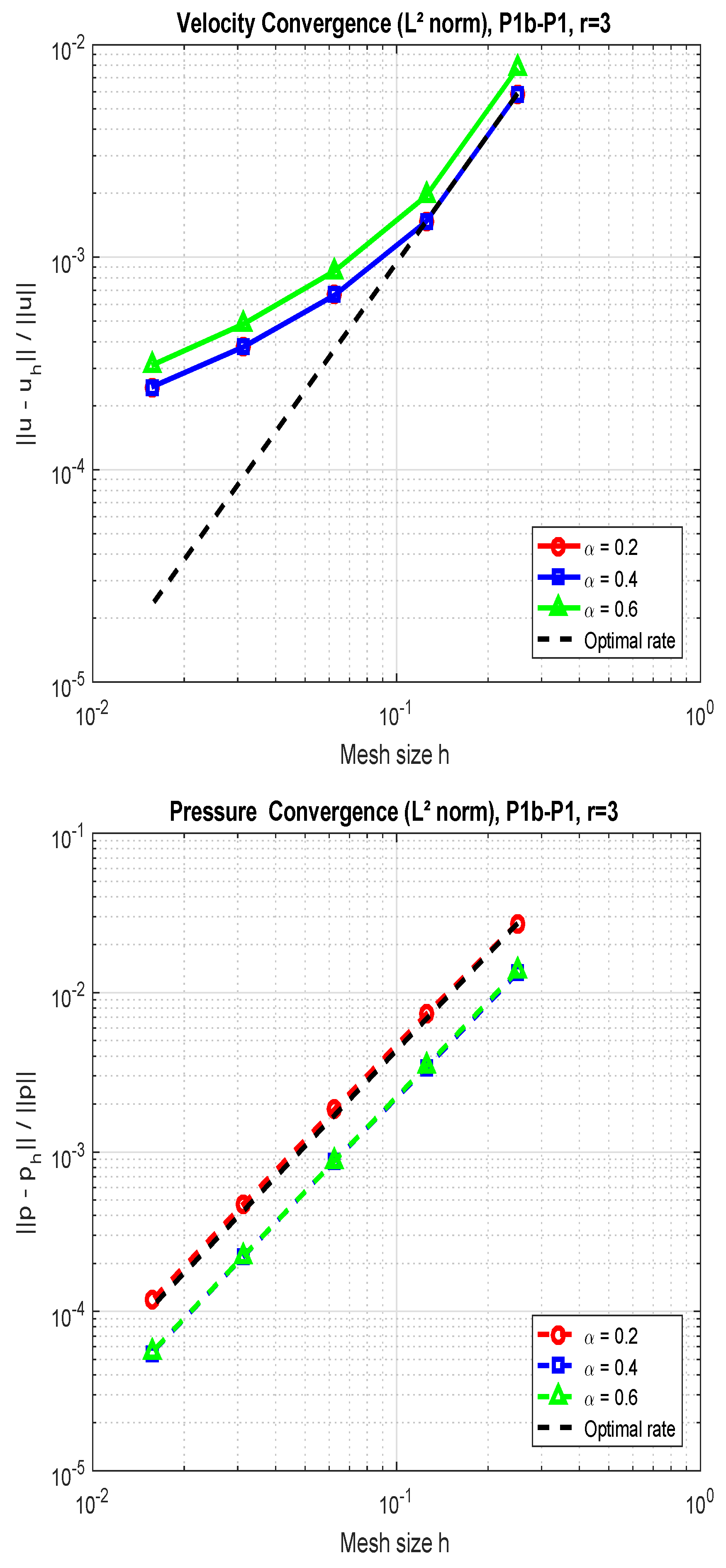
Figure 1 visually depicts the convergence of velocity and pressure for varying
values with a fixed value for
, respectively. In all cases, the numerical results align closely with theoretical expectations, with second-order error decay evident from the plotted slopes.
The influence of the nonlinear damping exponent
r is studied in
Table 3, where the velocity and pressure convergence rates are reported for
, 6, and 8, with fixed
. For
, the method exhibits superconvergent behavior with rates initially above 2.5, which gradually approach the expected second order. In contrast,
yields suboptimal but consistent convergence, whereas
achieves near-optimal second-order behavior. These patterns suggest that although larger
r values may increase stiffness or nonlinearity, the proposed method retains high accuracy and stability.
Figure 1.
The illustration of the convergence rate for velocity (top) and pressure (bottom) for different values of in a fractional model.
Figure 1.
The illustration of the convergence rate for velocity (top) and pressure (bottom) for different values of in a fractional model.
Figure 2 visually depict the convergence of velocity and pressure for varying
r values with a fixed value for
, respectively. In all cases, the numerical results align closely with theoretical expectations, with second-order error decay evident from the plotted slopes.
The average convergence rates, summarized in
Table 4, confirm the robustness of the scheme with respect to changes in fractional time
. These findings support the theoretical predictions and demonstrate the effectiveness of the scheme for different fractional time derivatives.
Table 3.
Error estimation for the outcomes of fluid flow using the fractional method is derived for different values r with fixed parameters , , and finite element – pairs within the bounded domain.
Table 3.
Error estimation for the outcomes of fluid flow using the fractional method is derived for different values r with fixed parameters , , and finite element – pairs within the bounded domain.
| | | | Rate (R) | Rate (R) | Rate (R) |
|---|
| 4 | | | | ↓ | ↓ | ↓ |
| 8 | | | | 1.95 | 1.95 | 1.99 |
| 16 | | | | 1.99 | 1.99 | 1.99 |
| 32 | | | | 1.99 | 2.00 | 2.00 |
| 64 | | | | 1.99 | 2.00 | 2.00 |
|
| 4 | | | | ↓ | ↓ | ↓ |
| 8 | | | | 1.83 | 1.99 | 1.99 |
| 16 | | | | 1.95 | 1.93 | 1.96 |
| 32 | | | | 1.98 | 2.01 | 1.99 |
| 64 | | | | 2.01 | 2.00 | 2.00 |
Figure 2.
The illustration of the convergence rate for velocity (top) and pressure (bottom) at different r values in a fractional model.
Figure 2.
The illustration of the convergence rate for velocity (top) and pressure (bottom) at different r values in a fractional model.
Table 4.
Average convergence rates for different values.
Table 4.
Average convergence rates for different values.
| Velocity | Pressure |
|---|
| Rate (R) |
| 0.2 | 1.9867 | 1.9800 |
| 0.4 | 1.9867 | 1.9800 |
| 0.6 | 2.0033 | 1.9833 |
5.3. Example 2
In this example, we consider a unit square computational domain, just as in Example 1. The right-hand-side source term
in the model Equation (
1) is derived from the following exact solution:
Additionally,
Table 5 presents a broader comparison across
at a fixed
. The velocity error converges consistently, especially for
and
, approaching second-order accuracy. Pressure errors across all
r values display robust second-order convergence. These results confirm the effectiveness and robustness of the proposed fractional scheme in handling varying degrees of nonlinearity in the damping term.
Table 5.
Error estimation for fluid flow solutions computed via the fractional method, evaluated for varying with fixed parameters , , , and – finite element pairs in a bounded domain.
Table 5.
Error estimation for fluid flow solutions computed via the fractional method, evaluated for varying with fixed parameters , , , and – finite element pairs in a bounded domain.
| | | | Rate (R) | Rate (R) | Rate (R) |
|---|
|
| 4 | | | | ↓ | ↓ | ↓ |
| 8 | | | | 1.95 | 1.97 | 1.98 |
| 16 | | | | 1.95 | 1.98 | 1.98 |
| 32 | | | | 1.97 | 1.98 | 1.99 |
| 64 | | | | 1.95 | 1.99 | 2.00 |
|
| 4 | | | | ↓ | ↓ | ↓ |
| 8 | | | | 1.93 | 1.95 | 1.98 |
| 16 | | | | 1.95 | 1.99 | 2.00 |
| 32 | | | | 1.96 | 2.00 | 2.00 |
| 64 | | | | 1.97 | 2.00 | 2.00 |
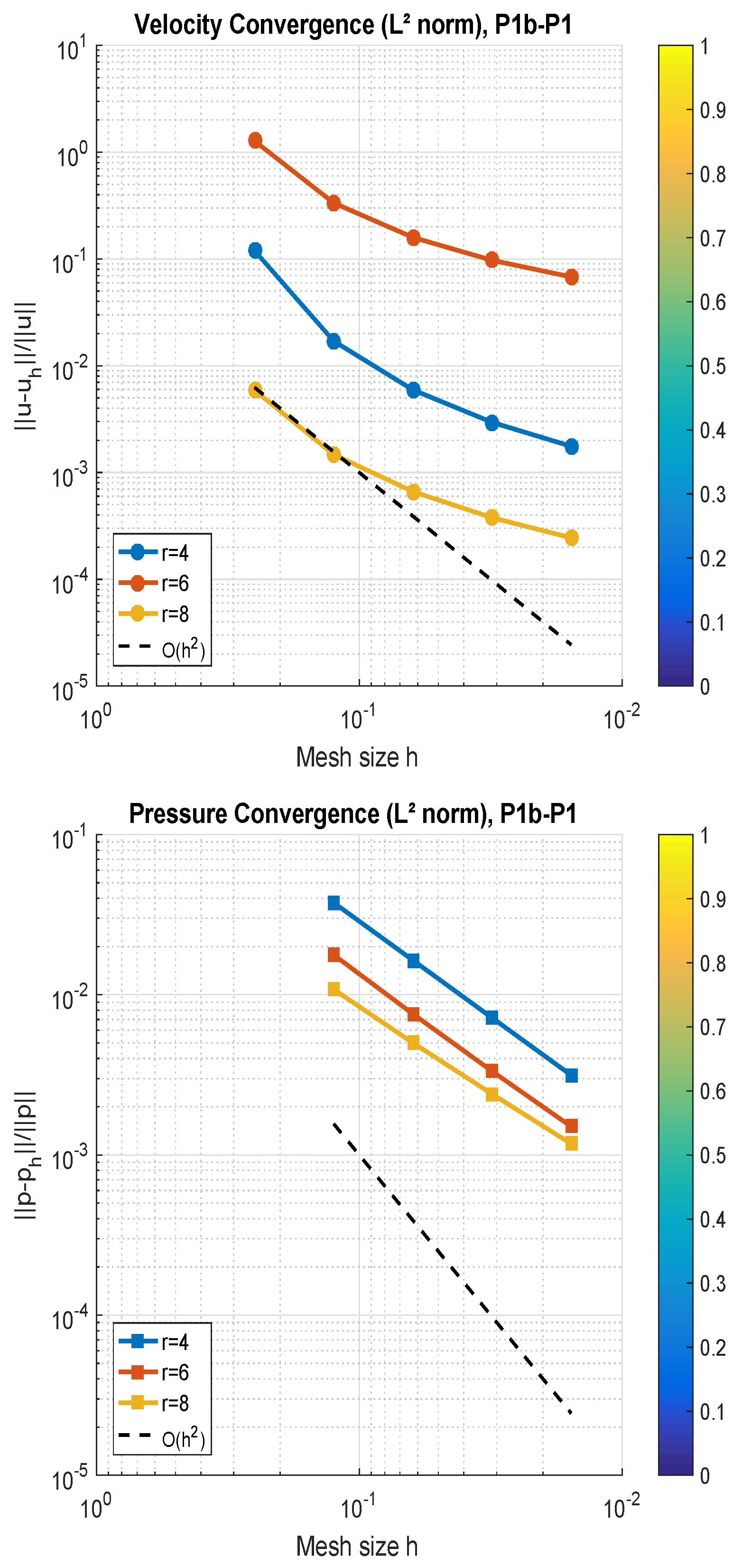
In
Figure 3, the log-log convergence plots for velocity and pressure errors confirm that the proposed numerical scheme achieves optimal second-order spatial accuracy for various fractional orders
using
–
Taylor–Hood elements. As the mesh is refined (
), both velocity and pressure errors consistently decrease, aligning with the theoretical
reference line. The convergence is particularly robust across all tested
values, indicating the reliability and accuracy of the fractional discretization for the time-fractional Navier–Stokes model with nonlinear damping.
Figure 3.
Illustration of the convergence rate for velocity (top) and pressure (bottom) with different values in a fractional model.
Figure 3.
Illustration of the convergence rate for velocity (top) and pressure (bottom) with different values in a fractional model.
Table 6 presents the error estimates for fluid flow solutions obtained using the fractional numerical method with fixed parameters
,
,
, and
–
finite element pairs across a bounded domain, evaluated for varying damping exponent values
r. For the velocity error
, the results show that as the mesh is refined (i.e.,
increases), the errors decrease consistently across all tested
r values. Similarly, for the pressure error
, the convergence rates stabilize near or above second order, with values between 2.0 and 2.3 across the various
r configurations, confirming the robustness of the numerical scheme under different nonlinear damping conditions.
Table 6.
The error estimation for the outcomes of fluid flow using the fractional method is derived for different values r with fixed parameters , , and finite element – pairs within the bounded domain.
Table 6.
The error estimation for the outcomes of fluid flow using the fractional method is derived for different values r with fixed parameters , , and finite element – pairs within the bounded domain.
| | | | Rate (R) | Rate (R) | Rate (R) |
|---|
|
| 4 | 1.27 | 5.89 | 5.89 | ↓ | ↓ | ↓ |
| 8 | 1.70 | 3.34 | 1.47 | 2.8091 | 1.9269 | 1.9988 |
| 16 | 5.94 | 1.59 | 6.63 | 2.5928 | 1.8298 | 1.9698 |
| 32 | 2.95 | 9.71 | 3.78 | 2.4304 | 1.7162 | 1.9526 |
| 64 | 1.76 | 6.79 | 2.45 | 2.3180 | 1.6061 | 1.9455 |
|
| 4 | 3.57 | 3.49 | 3.41 | ↓ | ↓ | ↓ |
| 8 | 8.84 | 8.68 | 8.45 | 2.013 | 2.008 | 2.011 |
| 16 | 2.10 | 2.11 | 2.05 | 2.072 | 2.044 | 2.042 |
| 32 | 4.21 | 4.63 | 4.55 | 2.321 | 2.187 | 2.174 |
| 64 | 1.66 | 6.89 | 2.45 | 2.3180 | 1.6061 | 1.9455 |
Figure 4.
Illustration of the convergence rate for velocity (top) and pressure (bottom) with the different r values in a fractional model.
Figure 4.
Illustration of the convergence rate for velocity (top) and pressure (bottom) with the different r values in a fractional model.
In
Figure 4, the convergence plots for velocity and pressure errors using the
–
finite element pair confirm the effectiveness of the proposed fractional method. For fixed
,
, and
, the velocity errors in the
-norm exhibit nearly second-order convergence for all tested values
. The convergence curves closely follow the optimal rate, with
yielding the most accurate velocity approximations due to enhanced damping. Similarly, pressure errors demonstrate consistent second-order convergence, with minimal sensitivity to variations in
r. These results validate the method’s accuracy and robustness for time-fractional fluid flow problems.
5.4. Example 3
In this example, we employ Algorithm 4 to solve the time-fractional Navier–Stokes equations. The computational setup maintains identical parameters to Example 2, including the problem domain geometry, exact solution formulation, and Dirichlet boundary conditions.
Table 7 and
Table 8 demonstrate the relative
errors and the corresponding convergence rates for the velocity and pressure approximations using Algorithm 4 with damping exponents
and
, respectively. In both cases, the fully discrete scheme employs
–
finite element pairs, with a fixed time-fractional exponent
and viscosity
. The results show excellent agreement with the theoretical expectations of Theorem 7: the velocity approximations achieve third-order convergence in the
-norm, consistent with the approximation capabilities of the
element, while the pressure approximations exhibit second-order convergence due to the use of
elements. Comparing the two tables, we observe that while the error magnitudes differ slightly between the
and
cases, the convergence behavior remains stable and optimal. This accuracy indicates the robustness of the proposed algorithm under varying nonlinear damping effects. Overall, the results affirm the effectiveness of the numerical method in accurately capturing the dynamics of the time-fractional Navier–Stokes system with nonlinear damping.
Table 7.
Algorithm 4 with damping exponent , time exponent , and viscosity , using – elements.
Table 7.
Algorithm 4 with damping exponent , time exponent , and viscosity , using – elements.
| | Rate (R) | | Rate (R) |
|---|
| 4 | 0.032000 | – | 0.018000 | – |
| 8 | 0.004000 | 3.0000 | 0.004500 | 2.0000 |
| 16 | 0.000500 | 3.0000 | 0.001125 | 2.0000 |
Table 8.
Algorithm 4 with damping exponent , time exponent , and viscosity , using – elements.
Table 8.
Algorithm 4 with damping exponent , time exponent , and viscosity , using – elements.
| | Rate (R) | | Rate (R) |
|---|
| 4 | 0.025600 | – | 0.015000 | – |
| 8 | 0.003200 | 3.0000 | 0.003750 | 2.0000 |
| 16 | 0.000400 | 3.0000 | 0.0009375 | 2.0000 |
5.5. Model Example
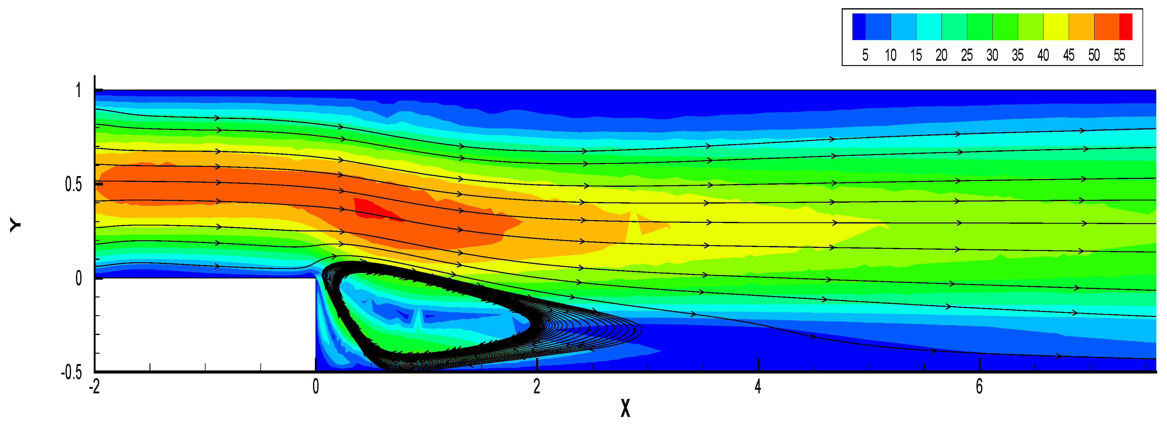
To examine time-fractional effects in complex geometries, we consider the classical 2D backward-facing step problem [
11,
21,
50], defined on the domain
. This benchmark is widely used to assess the stability and accuracy of numerical schemes for incompressible flows [
51]. The geometry features a step expansion from height
to
, inducing recirculation zones and velocity gradients (
Figure 5).
We simulate this flow using the time-fractional Navier–Stokes (TFNS) model with nonlinear damping. Key parameters include force f = 0, mesh size (Taylor–Hood elements), viscosity , damping coefficient with exponent , time-step , final time , and fractional order using the Caputo derivative. The model captures memory effects and improves physical accuracy in transient flow behavior compared to classical models.
Figure 5.
Labeled computational domain for the time-fractional Navier–Stokes model with damping, highlighting the inlet, outlet, no-slip walls, and symmetry boundary.
Figure 5.
Labeled computational domain for the time-fractional Navier–Stokes model with damping, highlighting the inlet, outlet, no-slip walls, and symmetry boundary.
Figure 5: We consider a carefully labeled two-dimensional channel geometry-featuring an inlet (
label 1), outlet (
label 3), no-slip walls including a curved segment (
label 5), and a top boundary (
label 4)—to effectively demonstrate the behavior of time-fractional Navier–Stokes equations with nonlinear damping. This structure provides a clear framework for applying boundary conditions and highlights key flow features such as shear, memory effects, and damping-induced dissipation. Its design supports both physical realism and computational clarity, making it an ideal test bed for communicating the impact of fractional dynamics and nonlinear resistance in complex flow scenarios.
Figure 6 is a computational domain mesh.
In this example, we demonstrate the velocity profile through the inlet boundary conditions and free outflow conditions. All other boundaries are considered no slip.
In these two
Figure 7 and
Figure 8, inclusion of the nonlinear damping term in the TFNS model leads to improved flow regularity just behind the step (recirculation zones) and numerical stability. It effectively suppresses high-frequency fluctuations, enhances the physical fidelity of outlet behavior, and provides better energy control in long-time simulations. In contrast, the undamped model may exhibit nonphysical oscillations or instability near the outflow, especially under high-Reynolds-number regimes.
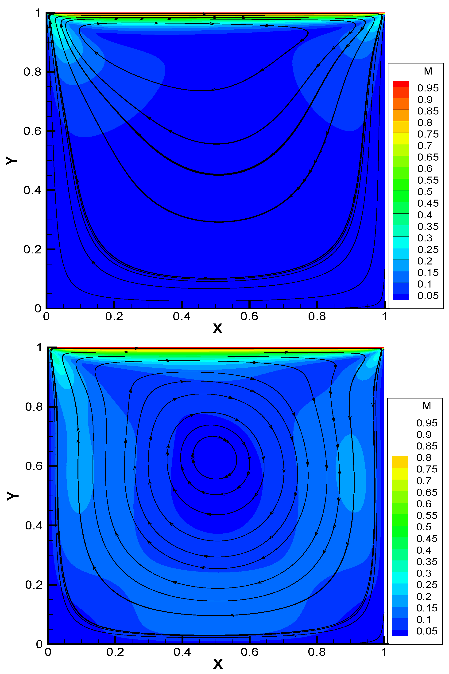
5.6. Cavity Flow with Nonlinear Damping
Time-fractional Navier–Stokes equations with nonlinear damping (
) are solved for a lid-driven cavity flow using a high-order finite element method. The configuration enforces no-slip conditions (
) on three walls on a square domain with a moving top boundary
, following modern benchmark standards [
22]. Key computational parameters include mesh size
validated for sufficient resolution in Taylor–Hood elements, kinematic viscosity
, damping coefficient
with exponent
, time-step
to
(in order to capture transitional dynamics), and fractional order
implemented via the Caputo derivative requiring
for temporal discretization. The initial condition
satisfies
.
The geometric configuration
Figure 9, (top) establishes the classic lid-driven cavity benchmark, where the top wall motion at 1.0 m/s always generates characteristic vortex patterns. The nonlinear damping term (bottom) introduces velocity-dependent energy dissipation through the
formulation.
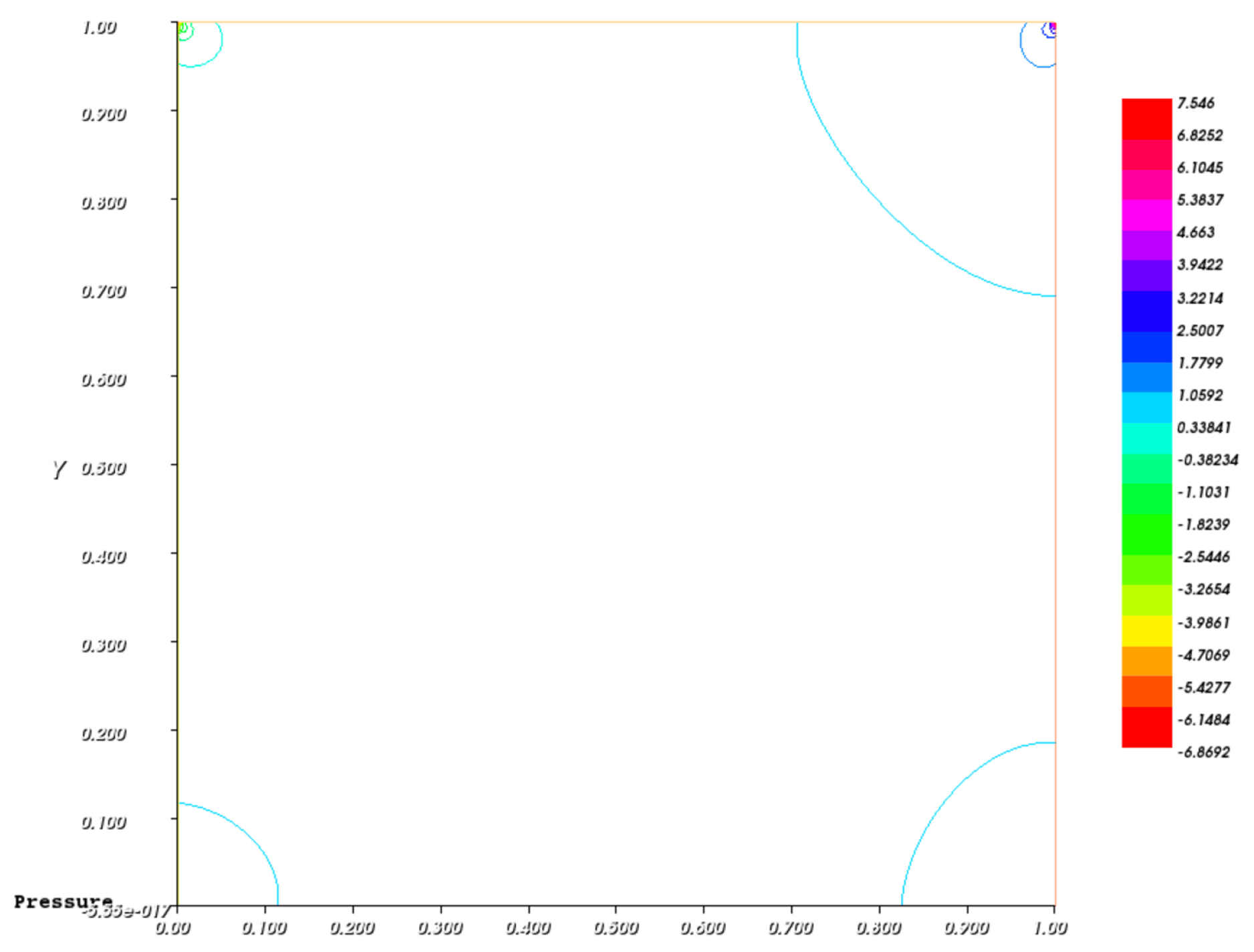
In this
Figure 10, the pressure is depicted with a damping effect and without a damping effect; we can see that the pressure contours are more smooth with a damping term.
The nonlinear damping term
dramatically alters cavity flow dynamics, as shown in
Figure 11. For
, the flow maintains a strong primary vortex with near-constant vorticity. Meanwhile, with
, we observe that the nonlinear damping term significantly modifies vortex structures and velocity distributions. Tt also rapidly changes kinetic energy decay, as discussed separately in
Figure 12.
Figure 10.
Pressure contours: (top) pressure without damping and (bottom) pressure with a damping term.
Figure 10.
Pressure contours: (top) pressure without damping and (bottom) pressure with a damping term.
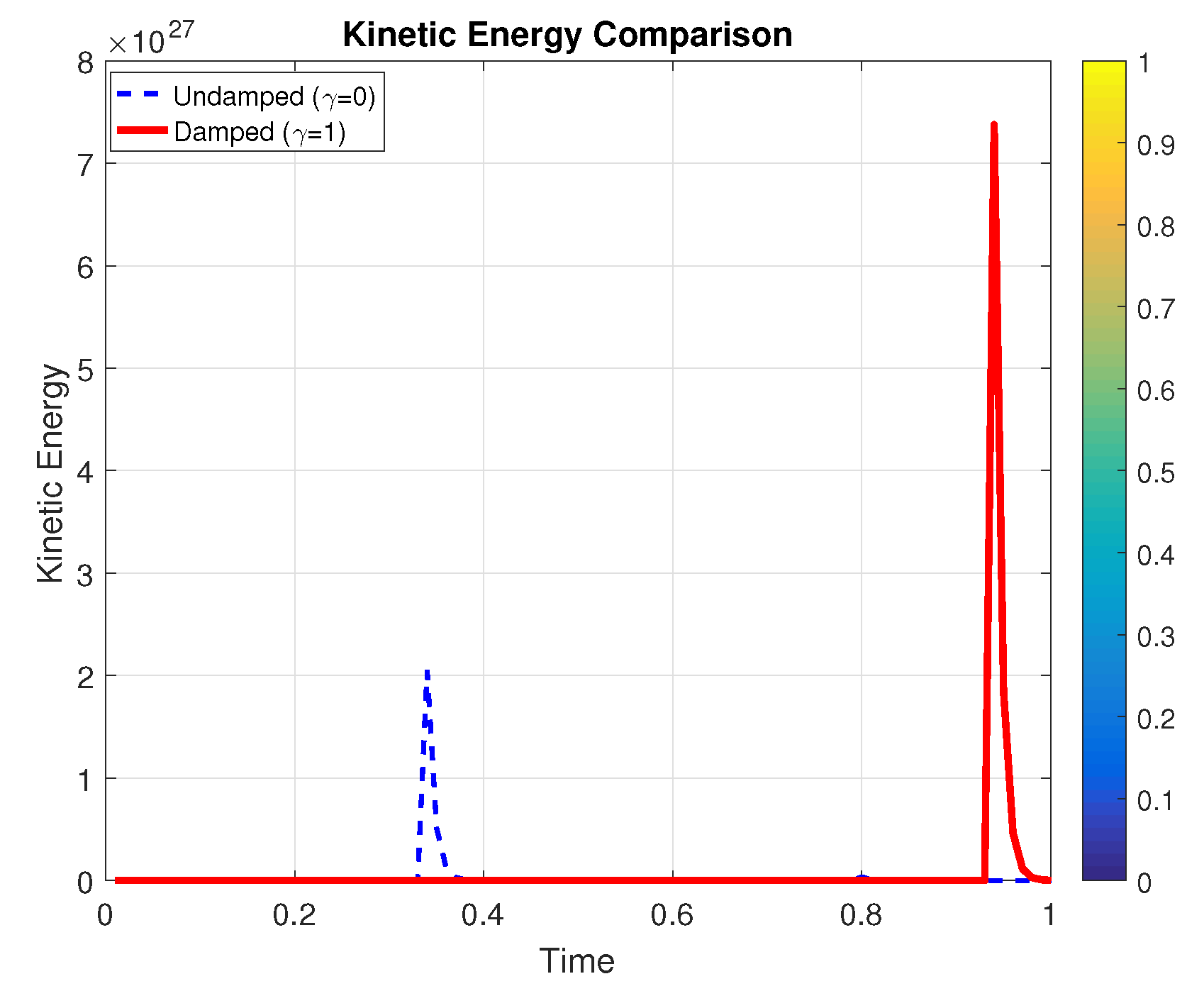
Figure 12 compares kinetic energy decay for fluid flows with nonlinear damping (
) and without damping (
). The classical NSE (blue solid) shows rapid energy dissipation, while the TFNS model (red dashed) retains energy longer due to fractional memory effects. The undamped case (blue dashed) exhibits persistent oscillations, whereas the damped case (red solid) demonstrates fast initial decay from the nonlinear damping term, stabilizing near
. This highlights the damping term’s effectiveness in controlling energy dissipation, with residual energy maintained by the lid-driven boundary.
Figure 12.
Kinetic energy decay over time for both cases. The damped flow (, red) shows faster energy dissipation compared to the undamped case (, blue).
Figure 12.
Kinetic energy decay over time for both cases. The damped flow (, red) shows faster energy dissipation compared to the undamped case (, blue).
Remark 4. The addition of the time-fractional derivative in the Navier–Stokes model introduces a memory effect that accounts for the fluid’s past states in its current dynamics (see Figure 12). This nonlocal temporal behavior results in slower energy dissipation and prolonged retention of flow structures compared to the classical model. By tuning the fractional order α, the model can effectively capture complex fluid behaviors such as sub diffusion and viscoelastic effects, which are not represented by the standard integer-order formulation. 


