A Structure-Preserving Finite Difference Scheme for the Nonlinear Space Fractional Sine-Gordon Equation with Damping Based on the T-SAV Approach

Abstract

This paper presents a high-order structure-preserving difference scheme for the nonlinear space fractional sine-Gordon equation with damping, employing the triangular scalar auxiliary variable approach. The original equation is reformulated into an equivalent system that satisfies a modified energy conservation or dissipation law, significantly reducing the computational complexity of nonlinear terms. Temporal discretization is achieved using a second-order difference method, while spatial discretization utilizes a simple and easily implementable discrete approximation for the fractional Laplacian operator. The boundedness and convergence of the proposed numerical scheme under the maximum norm are rigorously analyzed, demonstrating its adherence to discrete energy conservation or dissipation laws. Numerical experiments validate the scheme’s effectiveness, structure-preserving properties, and capability for long-time simulations for both one- and two-dimensional problems. Additionally, the impact of the parameter $\epsilon$ on error dynamics is investigated.

1. Introduction

By introducing the fractional derivative, the fractional-order nonlinear wave equation breaks through the limitations of the traditional integer-order model in describing complex physical phenomena such as non-local effects, anomalous diffusion, and remote interaction, and provides a more accurate modeling tool for quantum mechanics, fluid dynamics, and other fields. Recently, advances in fractional calculus have stimulated extensive research on both analytical and computational approaches to fractional partial differential equations [1,2,3,4]. A significant development in this field is the nonlinear fractional generalized wave equation, derived by generalizing classical hyperbolic equations through the integration of damping dynamics and fractional Laplacian operators within a fractional calculus framework. However, the non-locality and memory characteristics of the fractional-order operator lead to significant challenges in its numerical solution: the traditional low-order difference method has low computational efficiency, while the balance between accuracy and stability of the high-order method has not been effectively solved.

The space fractional sine-Gordon equation is in a class of nonlinear fractional generalized wave equations. It is an important dynamic model generalized from the classical sine-Gordon equation and used to describe long-range interactions in nonlinear science [5,6,7]. Since the fractional sine-Gordon equation has great advantages in describing the above phenomena, its numerical method has been widely studied [8,9,10]. For example, within the framework of the fractional sine-Gordon system, soliton and breather solution patterns were initially characterized by Korabel et al. [6]. Macías-Díaz [7] also revealed nonlinear supratransmission phenomena in space fractional sine-Gordon configurations through numerical verification.

This paper focuses on the following nonlinear space fractional sine-Gordon equation (NSFSGE):

$$\begin{array}{cc}\hfill & {\psi }_{tt}(x,t)+{\left(-\Delta \right)}^{\alpha /2}\psi (x,t)+\gamma {\psi }_t(x,t)+{\beta }^2\psi (x,t)+sin\left(\psi (x,t)\right)=0,\hfill \\ \hfill & \psi (x,0)=\epsilon u_0\left(x\right),{\psi }_t(x,0)=\epsilon u_1\left(x\right),x\in \overline{\Omega }.\hfill \end{array}$$

(1)

where the compact domain $x\in \Omega ={\prod }_{i=1}^d(a_i,b_i)\subset {\mathbb{R}}^d$, $d=1,2$ and $0<t\le T$. In this paper, we consider the homogeneous Dirichlet boundary conditions $\psi (x,t)=0$ for $x\in \partial \Omega .$ Here, $\gamma$ is a positive constant, $\psi (x,t)$ is a real-valued function, and $u_0\left(x\right)$ and $u_1\left(x\right)$ are two known real-valued initial functions that are independent of $\epsilon$. The operator ${(-\Delta )}^{\alpha /2}$, $1<\alpha \le 2$ is spatial fractional Laplacian defined by the following [11,12]:

$$\begin{array}{c}\hfill {(-\Delta )}^{\alpha /2}\psi (x,t)=c_{d,\alpha }P.V.\underset{{\mathbb{R}}^d}{\int }{\displaystyle \frac{\psi (x,t)-\psi (y,t)}{{|x-y|}^{d+\alpha }}}\mathrm{d}y,c_{d,\alpha }={\displaystyle \frac{2^{\alpha }\Gamma \left((\alpha +d)/2\right)}{{\pi }^{d/2}|\Gamma (-\alpha /2)|}}.\end{array}$$

(2)

When $\alpha =2$, $\gamma =\beta =0$, and $\epsilon =1$, the NSFSGE (1) is simplified to the classical sine-Gordon equation. Here, the dimensionless scaling factor $\epsilon \in (0,1)$ governs the nonlinear interaction intensity in Equation (1), which characterizes the nonlinear strength of Equation (1). When $\epsilon \ll 1$, the system is weakly nonlinear; when $\epsilon =1$, it degenerates into the standard nonlinear case. The lifetime of the solution can reach $O(1/{\epsilon }^2)$ [13].

For $0<\epsilon \le 1$, we introduce the scaled variables $u(x,t)=\psi (x,t)/\epsilon$ and $u_t(x,t)={\psi }_t(x,t)/\epsilon$; the NSFSGE (1) can be reformulated as

$$\begin{array}{cc}\hfill & u_{tt}(x,t)+{(-\Delta )}^{\alpha /2}u(x,t)+\gamma u_t(x,t)+{\beta }^{2}u(x,t)+{\displaystyle \frac{1}{\epsilon }}sin\left(\epsilon u(x,t)\right)=0,\hfill \\ \hfill & u(x,0)=u_0\left(x\right),u_t(x,0)=u_1\left(x\right).\hfill \end{array}$$

(3)

Consider the Taylor expansion $sin\left(u\right)=u-{\displaystyle \frac{u^3}{6}}+O\left(u^5\right)$. The first equation of (3) can rewritten as

$$u_{tt}(x,t)+{(-\Delta )}^{\alpha /2}u(x,t)+\gamma u_t(x,t)+{\beta }^{2}u(x,t)+u(x,t)-{\displaystyle \frac{{\epsilon }^2{u}^3(x,t)}{6}}=0.$$

The long-time dynamics of NSFSGE (1) are equivalent to those of NSFSGE (3). Therefore, we focus on analyzing the error estimates for the long-time dynamics of NSFSGE (3). The corresponding results can be straightforwardly extended to Equation (1).

When $\epsilon =1$, the NSFSGE (3) reduces to the classical NSFSGE, and there are many numerical studies on this [5,14,15,16,17]. Ran and Zhang [16] developed a fourth-order spatially accurate compact discretization scheme with second-order temporal convergence rates to solve the NSFSGE. Alfimov et al. [17] conducted numerical investigations into NSFSGE breather solutions using a rotating-wave approximation framework. Hu et al. [14] introduced a structure-preserving Fourier pseudo-spectral scheme that maintains essential dissipation properties for damped fractional sine-Gordon systems. In [18], a boundary element approach based on continuous linear elements was introduced to solve the two-dimensional sine-Gordon equation. Fu et al. [5] developed a structure-preserving linear implicit numerical scheme for NSFSGE, with rigorous analysis establishing the method’s stability and maximum norm convergence properties. However, these numerical methods and error estimates are generally still valid at $\mathrm{O}\left(1\right)$. When $0<\epsilon \ll 1$, the lifetime of the solution of NSFSGE (3) is $\mathrm{O}(1/{\epsilon }^2)$, and there are still relatively few research results related to this situation.

In the following analysis, we focus exclusively on the numerical methods and theoretical analysis of Equation (3). The equation exhibits energy dissipation or conservation characteristics. To formalize this behavior, define the energy functional $E\left(t\right)$ as

$$E\left(t\right)={\int }_{{\mathbb{R}}^d}{\left|{\displaystyle \frac{u(x,t)}{2}}\right|}^2+{\displaystyle \frac{1}{2}}{\left|{(-\Delta )}^{{\displaystyle \frac{1}{4}}}u(x,t)\right|}^2+{\displaystyle \frac{{\beta }^2}{2}}{\left|u(x,t)\right|}^2+{\displaystyle \frac{1}{{\epsilon }^2}}\left(1-cos\left(\epsilon u\right(x,t\left)\right)\right)\mathrm{d}x,$$

(4)

and then its derivative satisfies

$$E^{\prime }\left(t\right)=-\gamma {\int }_{{\mathbb{R}}^d}{\left|{\displaystyle \frac{\partial u(x,t)}{\partial t}}\right|}^2\mathrm{d}x\le 0,\forall t\in (0,T].$$

When $\gamma =0$, the energy is conserved. For $\gamma >0$, the energy dissipates over time.

The energy dissipation law will also serve as a key benchmark to evaluate numerical accuracy and stability. Within the computational science community, structure-preserving algorithms are widely acknowledged to outperform conventional numerical methodologies due to their capacity to retain critical intrinsic characteristics of the original dynamical system. The existing structure-preserving algorithms include the finite difference method, the finite element method, and so on. For example, Achouri’s work [19] focused on a two-dimensional fourth-order nonlinear wave equation, where a novel energy-preserving difference scheme was developed. Kadri [20] demonstrated the formulation of conservative linear numerical frameworks for fourth-order nonlinear strain wave systems through rigorous operator analysis. The triangular scalar auxiliary variable (T-SAV) method proposed by Yang et al. [21] is a new structure preservation technique. This methodology demonstrates significant efficacy in developing numerical formulations for diverse gradient flow systems, while effectively mitigating predominant limitations inherent in the conventional scalar auxiliary variable approach [22,23,24,25,26].

In this paper, we will propose an innovative structure preservation algorithm based on the T-SAV approach [21] for the NSFSGE, and establish the corresponding error analysis. The finite difference method is used for the fractional Laplacian operator in the spatial direction, and the second-order central difference method is used in the time direction. At the same time, we establish a direct link between computational error and the parameter $\epsilon$, the improved uniform error bound of the fully discrete scheme is verified, and the numerical method is verified to be suitable for long-time simulation via a numerical example. The structure of this paper is as follows: In Section 2, we combine the improved consistent error with the spatial fractional sine-Gordon equation, and transform Equation (3) into an equivalent system by introducing the T-SAV, and derive the modified energy conservation and dissipation property. In Section 3, we employ a temporal second-order central difference operator combined with a spatial fractional approximation method to discretize the equivalent system. We formulate a numerical framework and ultimately derive a conservative linear difference scheme. In Section 4, we prove the boundedness, convergence, and modified discrete dissipation energy law of the difference scheme. In Section 5, we present computational simulations to validate the analytical predictions derived from the theoretical framework. The principal findings and methodological advancements are systematically synthesized in Section 6.

2. Equivalent System Based on T-SAV Approach

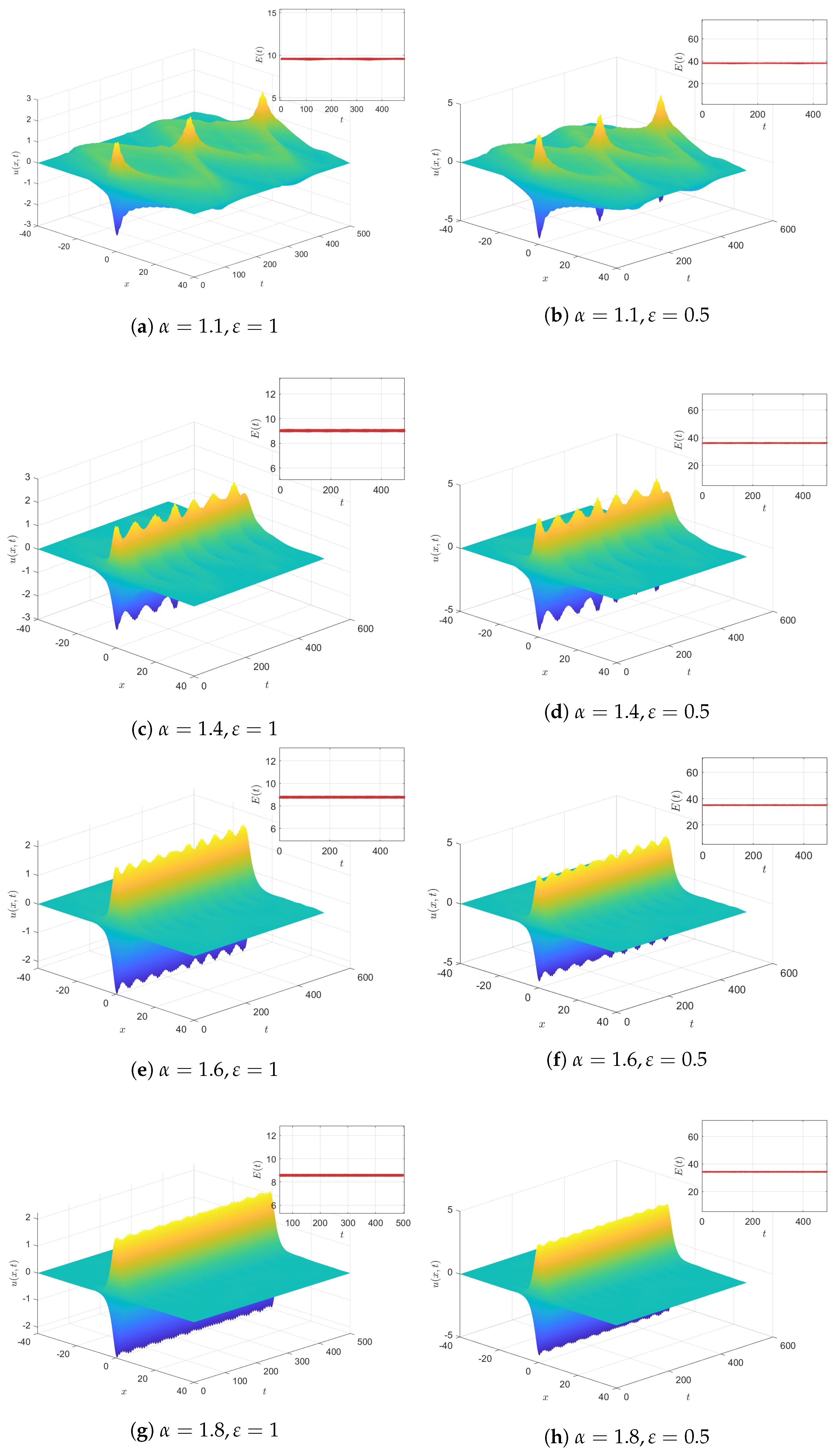
In this section, we reformulate the fractional sine-Gordon Equation (3) into an equivalent system obeying adjusted energy dissipation laws by T-SAV. The equivalent system provides a theoretical framework for the subsequent construction of high-order structure-preserving numerical schemes. Following the T-SAV approach [7], we define a scalar auxiliary variable:

$$r\left(t\right)=sin\left(F\right(t\left)\right)+C,$$

where $F\left(t\right)={\displaystyle \frac{1}{{\epsilon }^2}}{\int }_{\Omega }(1-cos\left(\epsilon u(x,t)\right))\mathrm{d}x$ and the constant $C>1$ serves as a stabilization parameter ensuring $r\left(t\right)>0$ for all t. Differentiating $r\left(t\right)$ with respect to time t yields

$${\displaystyle \frac{\mathrm{d}r\left(t\right)}{\mathrm{d}t}}=cos\left(F\left(t\right)\right)·{\displaystyle \frac{1}{\epsilon }}{\int }_{\Omega }sin\left(\epsilon u(x,t)\right)u_t(x,t)\mathrm{d}x.$$

Then, by using the trigonometric identity ${sin}^2\left(F\left(t\right)\right)+{cos}^2\left(F\left(t\right)\right)=1$, we can get

$${\displaystyle \frac{1}{\sqrt{1-{(r\left(t\right)-C)}^2}}}{\displaystyle \frac{\mathrm{d}r}{\mathrm{d}t}}={\displaystyle \frac{1}{\epsilon }}{\int }_{\Omega }sin\left(\epsilon u\right)u_t\mathrm{d}x,$$

which implies that

$${\displaystyle \frac{\mathrm{d}}{\mathrm{d}t}}\left(arcsin\left(r\right(t)-C)\right)={\displaystyle \frac{1}{\epsilon }}{\int }_{\Omega }sin\left(\epsilon u\right)u_t\mathrm{d}x={\displaystyle \frac{r}{\epsilon (sin(F\left(t\right))+C)}}{\int }_{\Omega }sin\left(\epsilon u\right)u_t\mathrm{d}x.$$

(5)

Therefore, System (3) with the nonlinear term ${\displaystyle \frac{1}{\epsilon }}sin\left(\epsilon u\right)$ can be equivalently rewritten as

$$\begin{array}{cc}\hfill & u_{tt}+{(-\Delta )}^{\alpha /2}u+\gamma u_t+{\beta }^{2}u+{\displaystyle \frac{r}{sin\left(F\right(t\left)\right)+C}}·{\displaystyle \frac{sin\left(\epsilon u\right)}{\epsilon }}=0,\hfill \\ \hfill & {\displaystyle \frac{\mathrm{d}}{\mathrm{d}t}}\left(arcsin\left(r\right(t)-C)\right)={\displaystyle \frac{r}{\epsilon (sin(F\left(t\right))+C)}}\langle sin\left(\epsilon u\right),u_t\rangle ,\hfill \end{array}$$

(6)

where the inner product on the space of measurable functions over $\Omega$ is defined by

$$\langle u,v\rangle ={\int }_{\Omega }uv\mathrm{d}x.$$

For notational simplicity, we define $b\left(u\right)={\displaystyle \frac{sin\left(\epsilon u\right)}{\epsilon (sin(F\left(t\right))+C)}}$. Then Equation (6) can be reformulated as

$$\begin{array}{cc}\hfill & u_{tt}+{(-\Delta )}^{\alpha /2}u+\gamma u_t+{\beta }^{2}u+r\left(t\right)b\left(u\right)=0,\hfill \\ \hfill & {\displaystyle \frac{\mathrm{d}}{\mathrm{d}t}}\left(arcsin\left(r\right(t)-C)\right)=\langle r\left(t\right)b\left(u\right),u_t\rangle .\hfill \end{array}$$

(7)

Theorem 1. 

The equivalent system (7) satisfies the following modified energy dissipation law

$${\displaystyle \frac{\mathrm{d}}{\mathrm{d}t}}\tilde{E}\left(t\right)=-\gamma {\parallel u_t\parallel }^2\le 0,$$

where the modified energy $\tilde{E}\left(t\right)$ is defined as

$$\tilde{E}\left(t\right)={\displaystyle \frac{1}{2}}\parallel u_t{\parallel }^2+{\displaystyle \frac{1}{2}}{\parallel (-\Delta )}^{\alpha /4}{u\parallel }^2+{\displaystyle \frac{{\beta }^2}{2}}{\parallel u\parallel }^2+arcsin(r\left(t\right)-C).$$

Proof. 

Differentiating $\tilde{E}\left(t\right)$ with respect to time t yields

$${\displaystyle \frac{\mathrm{d}}{\mathrm{d}t}}\tilde{E}\left(t\right)=〈u_t,u_{tt}〉+〈{(-\Delta )}^{\alpha /4}u,{(-\Delta )}^{\alpha /4}{u}_t〉+{\beta }^2〈u,u_t〉+{\displaystyle \frac{\mathrm{d}}{\mathrm{d}t}}arcsin(r\left(t\right)-C).$$

(8)

From the equivalent system given in (7), we obtain

$$u_{tt}=-{(-\Delta )}^{\alpha /2}u-\gamma u_t-{\beta }^{2}u-r\left(t\right)b\left(u\right).$$

(9)

Substituting (9) into (8) leads to

$$\begin{array}{cc}\hfill {\displaystyle \frac{\mathrm{d}}{\mathrm{d}t}}\tilde{E}& ={\int }_{\Omega }{u}_t\left[-{(-\Delta )}^{\alpha /2}u-\gamma u_t-{\beta }^{2}u-r\left(t\right)b\left(u\right)\right]\mathrm{d}x\hfill \\ \hfill & +〈{(-\Delta )}^{\alpha /4}u,{(-\Delta )}^{\alpha /4}{u}_t〉+{\beta }^2〈u,u_t〉+{\displaystyle \frac{\mathrm{d}}{\mathrm{d}t}}arcsin(r\left(t\right)-C).\hfill \end{array}$$

(10)

Since ${\int }_{\Omega }{u}_t{(-\Delta )}^{\alpha /2}u\mathrm{d}x=〈{(-\Delta )}^{\alpha /4}u,{(-\Delta )}^{\alpha /4}{u}_t〉$, from (10), it is easy to prove that

$${\displaystyle \frac{\mathrm{d}}{\mathrm{d}t}}\tilde{E}\left(t\right)=-\gamma {\parallel u_t\parallel }^2,$$

which completes the proof since $\gamma >0$. □

This result reveals two distinct physical regimes:

• When $\gamma =0$, it holds that ${\displaystyle \frac{\mathrm{d}\tilde{E}}{\mathrm{d}t}}=0$, indicating energy conservation in the system.
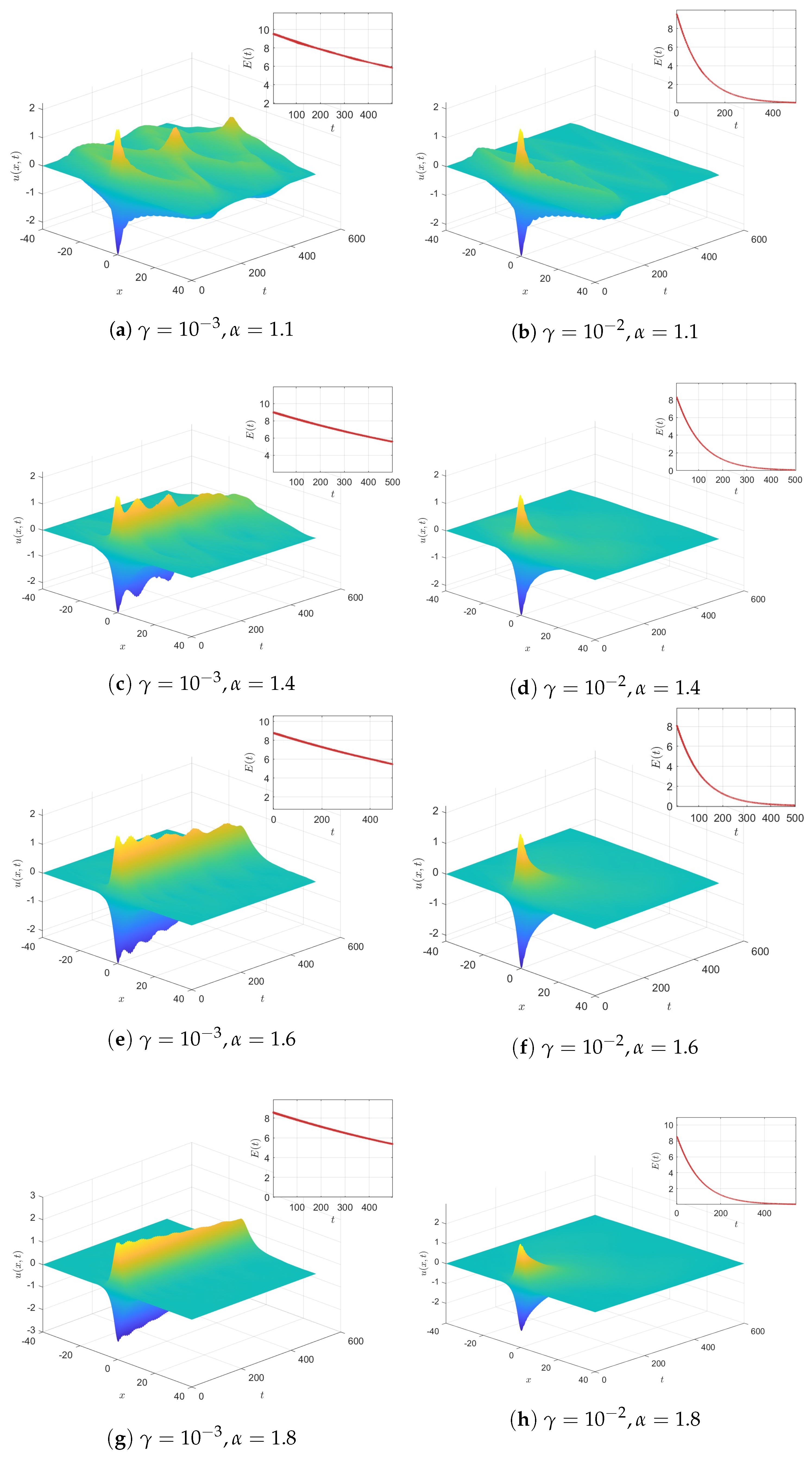
• When $\gamma >0$, the energy dissipates over time, demonstrating the physical effect of the damping term.

The transformation by introducing the T-SAV approach preserves the physical properties of the original system. The auxiliary variable $r\left(t\right)$ localizes the nonlinear term, so that the numerical discretization does not need to directly deal with complex nonlinear operators, which significantly improves the computational efficiency. This method lays a theoretical foundation for the subsequent construction of high-precision and structure-preserving numerical schemes. The next section will design a discrete difference scheme based on this equivalent system and analyze its properties.

3. Structure-Preserving Finite Difference Scheme

In this section, a high-order structure-preserving numerical scheme is designed for the NSFSGE (3), and a strict mathematical analysis is given.

3.1. Approximations for Spatial Fractional Laplacian

Let $V_h=\left\{u\right|u=(u_1,u_2,\cdots ,u_M)\}$ be the space of grid functions. For any two grid functions $u,v\in V_h$, define the discrete inner product and the associated norms as

$$\begin{array}{c}\hfill \langle u,v\rangle =h\sum _{i=1}^M{u}_i{v}_i,∥u∥=\sqrt{\langle u,u\rangle },{∥u∥}_{\infty }=\underset{1\le i\le M}{max}\left|u_i\right|.\end{array}$$

To approximate the spatial fractional Laplacian ${(-\Delta )}^{\alpha /2}$, in [27], a kind of discrete fractional Laplacian operator ${(-{\Delta }_h)}^{\alpha /2}$ is analyzed. In one-dimensional case, the centered difference approximation with step size h is

$${(-{\Delta }_h)}^{\alpha /2}u\left(x\right)={\displaystyle \frac{1}{h^{\alpha }}}\sum _{j\in \mathbb{Z}}{a}_j^{\left(\alpha \right)}u(x+jh),$$

(11)

where $a_j^{\left(\alpha \right)}$ gives expansion coefficients of the generating function ${\left[4{sin}^2\left({\displaystyle \frac{k}{2}}\right)\right]}^{\alpha /2}$, given as

$$\begin{array}{cc}\hfill a_j^{\left(\alpha \right)}& ={\displaystyle \frac{1}{2\pi }}{\int }_{-\pi }^{\pi }{\left[4{sin}^2\left({\displaystyle \frac{k}{2}}\right)\right]}^{\alpha /2}{e}^{-\mathrm{i}jk}\mathrm{d}k.\hfill \end{array}$$

The coefficients given by $a_j^{\left(\alpha \right)}$ can be evaluated using the trapezoidal rule; then, by considering the homogeneous Dirichlet boundary conditions, they are given by

$$\begin{array}{c}\hfill a_j^{\left(\alpha \right)}={\displaystyle \frac{1}{M}}\sum _{j=0}^{M-1}{\left[4{sin}^2\left({\displaystyle \frac{k}{2}}\right)\right]}^{\alpha /2}{e}^{-\mathrm{i}jk},\end{array}$$

where ${\mathrm{i}}^2=-1$. As proposed in [27], they also can be explicitly given in terms of Gamma functions as

$$\begin{array}{c}\hfill a_j^{\left(\alpha \right)}={\displaystyle \frac{{(-1)}^j\Gamma (\alpha +1)}{\Gamma (\alpha /2-j+1)\Gamma (\alpha /2+j+1)}}.\end{array}$$

(12)

For the two-dimensional case, the discrete fractional Laplacian operator can be generalized as follows:

$${(-{\Delta }_h)}_2^{\alpha /2}u(x,y):={\displaystyle \frac{1}{h^{\alpha }}}\sum _{i,j\in \mathbb{Z}}{a}_{i,j}^{\left(\alpha \right)}u(x+ih,y+jh),$$

(13)

where $a_{i,j}^{\left(\alpha \right)}$ gives the coefficients of the generating function ${[4{sin}^2\left({\displaystyle \frac{k_1}{2}}\right)+4{sin}^2\left({\displaystyle \frac{k_2}{2}}\right)]}^{\alpha /2}$, which can be expressed as

$$a_{i,j}^{\left(\alpha \right)}={\displaystyle \frac{1}{4{\pi }^2}}{\int }_{-\pi }^{\pi }{\int }_{-\pi }^{\pi }{[4{sin}^2\left({\displaystyle \frac{k_1}{2}}\right)+4{sin}^2\left({\displaystyle \frac{k_2}{2}}\right)]}^{\alpha /2}{e}^{-\mathrm{i}(i{k}_1+j{k}_2)}\mathrm{d}{k}_1\mathrm{d}{k}_2.$$

(14)

Define the Sobolev space $W^{s,1}\left({\mathbb{R}}^2\right)$ as

$$W^{s,1}\left({\mathbb{R}}^2\right)=\left\{u\mid u\in L^1\left({\mathbb{R}}^2\right),{\int }_{{\mathbb{R}}^2}{(1+|k\left|\right)}^s\left|\widehat{u}(k_1,k_2)\right|\mathrm{d}{k}_1\mathrm{d}{k}_2<\infty \right\}$$

where ${\left|k\right|}^2=k_1^2+k_2^2$. Then, if $u\in W^{\delta +\alpha ,1}\left({\mathbb{R}}^2\right)$ with a positive constant $\delta \le 2$ and $\widehat{u}(k_1,k_2)$ is the Fourier transform of $u(x,y)$. Then for the fractional centered difference operator ${(-{\Delta }_h)}_2^{\alpha /2}$ defined in (13), it holds that

$${(-\Delta )}_2^{\alpha /2}u(x,y)={(-{\Delta }_h)}_2^{\alpha /2}u(x,y)+O\left(h^{\delta }\right).$$

when h is sufficiently small.

Furthermore, it can be proved that there is a unique square root for the discrete fractional Laplacian ${(-{\Delta }_h)}^{\alpha /2}$.

Lemma 1 

([28]).There exists a unique square root ${(-{\Delta }_h)}^{\alpha /4}$ that satisfies the following square root decomposition condition, for any two grid functions $u,v\in V_h$.

$$〈{(-{\Delta }_h)}^{\alpha /2}u,v〉=〈{(-{\Delta }_h)}^{\alpha /4}u,{(-{\Delta }_h)}^{\alpha /4}v〉,$$

(15)

where ${(-{\Delta }_h)}^{\alpha /4}$ is symmetric positive definite.

It is noted that the convergence order of the approximation given in (14) to the fractional Laplacian is $\delta$, with $\delta \le 2$, which depends on the smooth conditions of u. Furthermore, the spatial fractional Laplacian ${(-\Delta )}^{\alpha /2}$ is equivalent to the Riesz fractional derivative in one-dimensional space. Therefore, the discrete fractional Laplacian ${(-{\Delta }_h)}^{\alpha /2}$ can also approximate the Riesz fractional derivative. However, the spatial fractional Laplacian is not equivalent to the Riesz derivative in two-dimensional space.

3.2. Derivation of Structure-Preserving Difference Scheme

Define temporal nodes as $t_n=n\tau$ with time step $\tau$ where $0<t_n\le T$. We denote the point-wise numerical solution as $u_j^n\approx u(x_j,t_n)$, numerical solution vector as $u^n={(u_1^n,u_2^n,\dots ,u_M^n)}^T$, point-wise exact solution as $U_j^n\approx U(x_j,t_n)$, exact solution vector as $U^n={(U_1^n,U_2^n,\dots ,U_M^n)}^T$, and the auxiliary variable as $r^n\approx r\left(t_n\right)$.

Define the following difference operator:

$$\begin{array}{cc}\hfill u_t& \approx {\delta }_t{u}^n:={\displaystyle \frac{u^{n+1}-u^{n-1}}{2\tau }},{\delta }_t^{+}{u}^n:={\displaystyle \frac{u^{n+1}-u^n}{\tau }},\hfill \end{array}$$

$$\begin{array}{cc}\hfill u_{tt}& \approx {\delta }_t^2{u}^n:={\displaystyle \frac{u^{n+1}-2u^n+u^{n-1}}{{\tau }^2}},{\widehat{u}}^n:={\displaystyle \frac{u^{n+1}+u^{n-1}}{2}},u^{n+{\displaystyle \frac{1}{2}}}:={\displaystyle \frac{u^{n+1}+u^n}{2}}.\hfill \end{array}$$

By discretizing the fractional Laplacian operator ${(-\Delta )}^{\alpha /2}$ via the finite difference operator ${(-{\Delta }_h)}^{\alpha /2}$, and discretizing the derivatives in time by using the second-order central difference operator ${\delta }_t^2$, we discretize Formula (7) as

$$\begin{array}{c}{\delta }_t^2{u}^n+{(-{\Delta }_h)}^{\alpha /2}{\widehat{u}}^n+\gamma {\delta }_t{u}^n+{\beta }^2{\widehat{u}}^n+r^{n}b\left(u^n\right)=0,\\ b\left(u^n\right)={\displaystyle \frac{sin\left(\epsilon u^n\right)}{\epsilon (sin\left(F^n\left(t\right)\right)+C)}},\end{array}$$

(16)

and the auxiliary variable update follows:

$${\delta }_t^{+}arcsin(r^n-C)=\langle r^{n}b\left(u^n\right),{\delta }_t{u}^n\rangle .$$

(17)

To implement the proposed three-level scheme (16) and (17), we require initial values $u^0$ and $u^1$. While $u^0=u_0$ is directly given by Equation (3), the determination of $u^1$ necessitates additional analysis.

Setting $t=0$ in Equation (3) gives

$$U_{tt}^0=-\left({(-\Delta )}^{\alpha /2}{U}^0+\gamma U_t^0+{\beta }^2{U}^0+{\displaystyle \frac{sin\left(\epsilon U^0\right)}{\epsilon }}\right).$$

Performing a Taylor expansion of $U^1$ at $t=0$ yields

$$\begin{array}{cc}\hfill U^1& =U^0+\tau U_t^0+{\displaystyle \frac{{\tau }^2}{2}}{U}_{tt}^0+\mathcal{O}\left({\tau }^3\right)\hfill \\ \hfill & =U^0+\tau U_t^0-{\displaystyle \frac{{\tau }^2}{2}}\left({(-\Delta )}^{\alpha /2}{U}^0+\gamma U_t^0+{\beta }^2{U}^0+{\displaystyle \frac{sin\left(\epsilon U^0\right)}{\epsilon }}\right)+\mathcal{O}\left({\tau }^3\right).\hfill \end{array}$$

(18)

Substituting the Taylor expansion of the sine function into the nonlinear term, we can get

$$\begin{array}{cc}\hfill {\displaystyle \frac{1}{\epsilon }}sin\left(\epsilon U^0\right)& =U^0-{\displaystyle \frac{{\epsilon }^2}{6}}{\left(U^0\right)}^3+\mathcal{O}\left({\epsilon }^4{\left(U^0\right)}^5\right)\hfill \\ \hfill & =U^0-{\displaystyle \frac{{\epsilon }^2}{6}}{\left(U^0+\mathcal{O}\left(\tau \right)\right)}^3+\mathcal{O}\left({\epsilon }^4{\left(U^0\right)}^5\right)\hfill \\ \hfill & =U^0-{\displaystyle \frac{{\epsilon }^2}{6}}{\left(U^0\right)}^3+\mathcal{O}\left(\tau \right).\hfill \end{array}$$

(19)

Substituting the expansion in (19) of the nonlinear term and the initial value condition in (3) into (18), and replacing the exact solution by a numerical solution, we obtain

$$\begin{array}{cc}\hfill u^1& =u^0+\tau u_t^0-{\displaystyle \frac{{\tau }^2}{2}}\left({(-{\Delta }_h)}^{\alpha /2}{u}^0+\gamma u_t^0+{\beta }^2{u}^0+{\displaystyle \frac{sin\left(\epsilon u^0\right)}{\epsilon }}\right)\hfill \\ \hfill & =u^0+\tau u_1-{\displaystyle \frac{{\tau }^2}{2}}\left({(-{\Delta }_h)}^{\alpha /2}{u}^0+\gamma u_1+{\beta }^2{u}^0+u^0-{\displaystyle \frac{{\epsilon }^2}{6}}{\left(u^0\right)}^3\right),\hfill \end{array}$$

which leads to

$${\displaystyle \frac{u^1-u^0}{\tau }}+{\displaystyle \frac{\tau }{2}}\left({(-{\Delta }_h)}^{\alpha /2}{u}^0+\gamma u_1+({\beta }^2+1)u^0-{\displaystyle \frac{{\epsilon }^2}{6}}{\left(u^0\right)}^3\right)=u_1.$$

(20)

Then, the initial value $u^1$ required to start the numerical schemes (16) and (17) can be determined by the following scheme:

$${\delta }_t^{+}{u}^0+{\displaystyle \frac{\tau }{2}}{(-{\Delta }_h)}^{\alpha /2}{u}^0+{\displaystyle \frac{({\beta }^2+1)\tau }{2}}{u}^0-{\displaystyle \frac{\tau {\epsilon }^2}{12}}{\left(u^0\right)}^3=\left(1-{\displaystyle \frac{\gamma \tau }{2}}\right)u_1.$$

(21)

4. Numerical Analysis

In this section, the boundedness, convergence, and modified discrete energy dissipation law of the numerical solution for the NSFSGEs are analyzed in detail.

4.1. Discrete Energy Dissipation Law

Theorem 2. 

The difference scheme (16) and (17) satisfies the following modified discrete energy dissipation law:

$$E_h^{n+1}-E_h^n=-\gamma \tau {∥{\delta }_t{u}^n∥}^2,$$

(22)

where the discrete energy is defined as

$$\begin{array}{cc}\hfill E_h^{n+1}& ={\displaystyle \frac{1}{2}}{∥{\delta }_t^{+}{u}^n∥}^2+{\displaystyle \frac{1}{4}}\left({∥{(-{\Delta }_h)}^{\alpha /4}{u}^{n+1}∥}^2+{∥{(-{\Delta }_h)}^{\alpha /4}{u}^n∥}^2\right)\hfill \\ \hfill & +{\displaystyle \frac{{\beta }^2}{4}}\left({∥u^{n+1}∥}^2+{∥u^n∥}^2\right)+arcsin(r^{n+1}-C).\hfill \end{array}$$

(23)

Proof. 

Subtracting $E_h^n$ from $E_h^{n+1}$ defined in (23) leads to

$$\begin{array}{cc}\hfill E_h^{n+1}-E_h^n& ={\displaystyle \frac{1}{2}}\left({∥{\delta }_t^{+}{u}^n∥}^2-{∥{\delta }_t^{+}{u}^{n-1}∥}^2\right)+{\displaystyle \frac{1}{4}}\left({∥{(-{\Delta }_h)}^{\alpha /4}{u}^{n+1}∥}^2-{∥{(-{\Delta }_h)}^{\alpha /4}{u}^{n-1}∥}^2\right)\hfill \\ \hfill & +{\displaystyle \frac{{\beta }^2}{4}}\left({∥u^{n+1}∥}^2-{∥u^{n-1}∥}^2\right)+arcsin(r^{n+1}-C)-arcsin(r^n-C).\hfill \end{array}$$

Taking the inner product of the difference scheme (16) with ${\delta }_t{u}^n$ yields

$$\begin{array}{c}\hfill 〈{\delta }_t^{+}{u}^n,{\delta }_t{u}^n〉+〈{(-{\Delta }_h)}^{\alpha /2}{u}^n,{\delta }_t{u}^n〉+\gamma 〈{\delta }_t{u}^n,{\delta }_t{u}^n〉+{\beta }^2〈u^n,{\delta }_t{u}^n〉+〈b\left(u^n\right)r^n,{\delta }_t{u}^n〉=0.\end{array}$$

(24)

A simple calculation shows that the following identities hold:

$$\begin{array}{cc}\hfill & 〈{\delta }_t^2{u}^n,{\delta }_t{u}^n〉={\displaystyle \frac{1}{2\tau }}\left({∥{\delta }_t^{+}{u}^n∥}^2-{∥{\delta }_t^{+}{u}^{n-1}∥}^2\right),\hfill \end{array}$$

(25)

$$\begin{array}{cc}\hfill & 〈{(-{\Delta }_h)}^{\alpha /2}{\widehat{u}}^n,{\delta }_t{u}^n〉={\displaystyle \frac{1}{4\tau }}\left({∥{(-{\Delta }_h)}^{\alpha /4}{u}^{n+1}∥}^2-{∥{(-{\Delta }_h)}^{\alpha /4}{u}^{n-1}∥}^2\right),\hfill \end{array}$$

(26)

$$\begin{array}{cc}\hfill & \gamma 〈{\delta }_t{u}^n,{\delta }_t{u}^n〉=\gamma \tau {∥{\delta }_t{u}^n∥}^2,\hfill \end{array}$$

(27)

$$\begin{array}{cc}\hfill & {\beta }^2〈{\widehat{u}}^n,{\delta }_t{u}^n〉={\displaystyle \frac{{\beta }^2}{4\tau }}\left({∥u^{n+1}∥}^2-{∥u^{n-1}∥}^2\right).\hfill \end{array}$$

(28)

Substituting (25)–(28) and (17) into (24) yields

$$E_h^{n+1}-E_h^n=\tau \left[〈{\delta }_t^2{u}^n+{(-{\Delta }_h)}^{\alpha /2}{u}^n+{\beta }^2{u}^n+b\left(u^n\right)r^n,{\delta }_t{u}^n〉\right].$$

Combining with the scheme in (16), we obtain the energy dissipation law given in (22), which completes the proof. □

4.2. Boundedness

Theorem 3. 

The numerical solution $u^n$ is uniformly bounded in the maximum norm. That is, there exists a positive constant C independent of h and τ such that $\parallel u^n{\parallel }_{\infty }\le C.$

Proof. 

The theorem can be proved by mathematical induction and using the conserved properties of the modified energy.

For $n=0$, the initial function where $u_0\left(x\right)$ is an infinitely differentiable periodic function on $\Omega$. A key property of such functions is their uniform boundedness on closed intervals; we have that $\parallel u^0{\parallel }_{\infty }\le C_0$ with $C_0$ depends on the bound of $u_0$ but remains independent of h and $\tau$.

Assume that for all $0\le k\le n$, it holds that $\parallel u^k{\parallel }_{\infty }\le C$. According to Theorem 2, the modified discrete energy satisfies $E_h^{n+1}=E_h^n-\gamma \tau {∥{\delta }_t{u}^n∥}^2$. Then, combining the energy dissipation property $E_h^n\le E_h^0$ with the energy definition yields that

$$\begin{array}{c}\hfill {\displaystyle \frac{1}{2}}{∥{\delta }_t^{+}{u}^{n-1}∥}^2+{\displaystyle \frac{1}{4}}({∥{(-{\Delta }_h)}^{\alpha /4}{u}^n∥}^2+{∥{(-{\Delta }_h)}^{\alpha /4}{u}^{n-1}∥}^2)\\ \hfill +{\displaystyle \frac{{\beta }^2}{4}}({∥u^n∥}^2+{∥u^{n-1}∥}^2)\le E_h^0-arcsin(r^n-C).\end{array}$$

Since

$$-{\displaystyle \frac{\pi }{2}}\le arcsin(r^n-C)\le {\displaystyle \frac{\pi }{2}},$$

we further obtain

$$\begin{array}{cc}\hfill & {\displaystyle \frac{1}{2}}{∥{\delta }_t^{+}{u}^{n-1}∥}^2+{\displaystyle \frac{1}{4}}({∥{(-{\Delta }_h)}^{\alpha /4}{u}^n∥}^2+{∥{(-{\Delta }_h)}^{\alpha /4}{u}^{n-1}∥}^2)\hfill \\ & +{\displaystyle \frac{{\beta }^2}{4}}({∥u^n∥}^2+{∥u^{n-1}∥}^2)\le E_h^0-{\displaystyle \frac{\pi }{2}}.\hfill \end{array}$$

From $E_h^n\le E_h^0$, we have

$$\begin{array}{cc}\hfill {\displaystyle \frac{1}{2}}{∥{\delta }_t^{+}{u}^{n-1}∥}^2& \le E_h^0,{\displaystyle \frac{1}{4}}{∥{(-{\Delta }_h)}^{\alpha /4}{u}^n∥}^2\le E_h^0,{\displaystyle \frac{{\beta }^2}{4}}{∥u^n∥}^2\le E_h^0,\hfill \end{array}$$

Further simplification yields

$$\begin{array}{cc}\hfill ∥{(-{\Delta }_h)}^{\alpha /4}{u}^n∥& \le 2\sqrt{E_h^0},∥u^n∥\le 2\sqrt{{\displaystyle \frac{E_h^0}{{\beta }^2}}}.\hfill \end{array}$$

Then, by applying the discrete Sobolev inequality, we obtain

$${∥u^n∥}_{\infty }\le 2M_1\sqrt{E_h^0}+2M_2\sqrt{{\displaystyle \frac{E_h^0}{{\beta }^2}}}\le C.$$

(29)

The conclusion is proved by mathematical induction. □

4.3. Convergence

To analyze the conservation property of the present numerical method, the following discrete Grönwall inequality is needed.

Lemma 2 

([29]). Consider a discrete grid function $\{w^n\mid n=0,1,\cdots ,N=T/\tau \}$ satisfying the inequality

$$w^n-w^{n-1}\le A\tau w^n+B\tau w^{n-1}+C_n\tau ,$$

where $A,B,$ and $C_n$ are non-negative constants. Then, it holds that

$$\underset{1\le n\le N}{max}\left|w^n\right|\le \left(w^0+\tau \sum _{k=1}^N{C}_k\right)e^{2(A+B)T},$$

where τ is sufficiently small such that $(A+B)\tau \le {\displaystyle \frac{N-1}{2N}}<{\displaystyle \frac{1}{2}}$ for $N>1$.

Lemma 3 

([29]). For any grid function $u\in U_t$, we have the estimate

$$\parallel u\parallel \le {\displaystyle \frac{T}{\sqrt{6}}}\parallel {\delta }_t^{+}u\parallel .$$

Theorem 4. 

Assuming the exact solution $U(x,t)\in W^{2+\alpha ,1}(\Omega )\times (0.T)$, the discrete scheme given in (16) achieves second convergence order both in time and space in the maximum norm sense—i.e.,

$$\underset{0\le n\le T/\tau }{max}{∥U^n-u^n∥}_{\infty }\le C({\tau }^2+h^2),$$

where the constant C is independent of h and τ.

Proof. 

Define the error vector $e^n=U^n-u^n$, where $U^n={(U_1^n,U_2^n,\cdots ,U_M^n)}^T$ represents the exact solution values and $u^n$ denotes the numerical solution.

By subtracting the numerical solution obtained in (16) and (21) from the exact solution, we obtain the following error formula:

$$\begin{array}{cc}\hfill & {\delta }_t^2{e}^n+{(-{\Delta }_h)}^{\alpha /2}{\widehat{e}}^n+\gamma {\delta }_t{e}^n+{\beta }^2{\widehat{e}}^n+b\left(U^n\right)R^n-b\left(u^n\right)r^n=q^n,\hfill \end{array}$$

(30)

$$\begin{array}{cc}\hfill & {\delta }_t^{+}{e}^0+{\displaystyle \frac{\tau }{2}}{(-{\Delta }_h)}^{\alpha /2}{e}^0+{\displaystyle \frac{({\beta }^2+1)\tau }{2}}{e}^0-{\displaystyle \frac{{\epsilon }^2\tau }{12}}{\left(U^0\right)}^3+{\displaystyle \frac{{\epsilon }^2\tau }{12}}{\left(u^0\right)}^3=w,\hfill \end{array}$$

(31)

where $q^n={(q_1^n,q_2^n,\cdots ,q_M^n)}^T$ and $w={(w_1,w_2,\cdots ,w_M)}^T$ represent local truncation errors. Therefore, we get

$$\begin{array}{cc}\hfill & {\delta }_t^2{U}^n+{(-{\Delta }_h)}^{\alpha /2}{\widehat{U}}^n+\gamma {\delta }_t{U}^n+{\beta }^2{\widehat{U}}^n+b\left(U^n\right)r^n=q^n,\hfill \\ \hfill & {\delta }_t^{+}{U}^0+{\displaystyle \frac{\tau }{2}}{(-{\Delta }_h)}^{\alpha /2}{U}^0+{\displaystyle \frac{({\beta }^2+1)\tau }{2}}{U}^0-{\displaystyle \frac{{\epsilon }^2\tau }{12}}{\left(U^0\right)}^3=w,\hfill \end{array}$$

with the truncation errors bounded by $q^n\le c_4({\tau }^2+h^2)$, $w\le c_5({\tau }^3+h^2).$

Since the expressions of (31) for $n=0$ and (30) for $n\ge 1$ are different, we will discuss the convergence for the cases of $n=0$ and $n\ge 1$, respectively, in the following proof process.

Firstly, consider the case of $n=0$. Taking the inner product of (31) with ${\delta }_t^{+}{e}^0$, we obtain

$$\begin{array}{cc}\hfill 〈{\delta }_t^{+}{e}^0,{\delta }_t^{+}{e}^0〉& +{\displaystyle \frac{\tau }{2}}〈{(-{\Delta }_h)}^{\alpha /2}{e}^0,{\delta }_t^{+}{e}^0〉+{\displaystyle \frac{({\beta }^2+1)\tau }{2}}〈e^0,{\delta }_t^{+}{e}^0〉\hfill \\ & -{\displaystyle \frac{\tau }{2}}〈{\displaystyle \frac{{\epsilon }^2}{6}}\left({\left(U^0\right)}^3-{\left(u^0\right)}^3\right),{\delta }_t^{+}{e}^0〉=〈w,{\delta }_t^{+}{e}^0〉,\hfill \end{array}$$

(32)

It can be calculated that

$$\begin{array}{cc}\hfill & {\displaystyle \frac{\tau }{2}}〈{(-{\Delta }_h)}^{\alpha /2}{e}^0,{\delta }_t^{+}{e}^0〉={\displaystyle \frac{1}{2}}〈{(-{\Delta }_h)}^{\alpha /2}{e}^0,e^1-e^0〉=0,\hfill \\ \hfill & {\displaystyle \frac{({\beta }^2+1)\tau }{2}}〈e^0,{\delta }_t^{+}{e}^0〉={\displaystyle \frac{({\beta }^2+1)}{2}}〈e^0,e^1-e^0〉=0,\hfill \\ \hfill & {\displaystyle \frac{\tau }{2}}〈{\displaystyle \frac{{\epsilon }^2}{6}}({\left(U^0\right)}^3-{\left(u^0\right)}^3),{\delta }_t^{+}{e}^0〉={\displaystyle \frac{{\epsilon }^2}{12}}〈0,e^1-e^0〉=0.\hfill \end{array}$$

Substituting them into (32) yields

$${∥{\delta }_t^{+}{e}^0∥}^2=〈w,{\delta }_t^{+}{e}^0〉.$$

Since

$${\displaystyle \frac{{∥e^1∥}^2}{\tau }}\le {∥{\delta }_t^{+}{e}^0∥}^2,〈w,{\delta }_t^{+}{e}^0〉\le {\displaystyle \frac{1}{2}}\left({∥w∥}^2+{∥{\delta }_t^{+}{e}^0∥}^2\right),$$

we have

$${\displaystyle \frac{1}{2\tau }}{∥e^1∥}^2\le {\displaystyle \frac{1}{2}}{∥w∥}^2,$$

which implies

$${∥e^1∥}^2\le c_5^2\tau L{({\tau }^3+h^2)}^2\le c_5^{2}TL{({\tau }^3+h^2)}^2.$$

By using the discrete fractional Sobolev embedding theorem, there exists one constant $M_1$ such that

$$\parallel e^1{\parallel }_{\infty }\le \left(c_5{M}_1\sqrt{TL}\right){(h^2+{\tau }^3)}^2.$$

Secondly, consider the case of $n\ge 1$. Applying the mean value theorem $f\left(b\right)-f\left(a\right)=f^{\prime }\left(c\right)(b-a)$ to the nonlinear term $sin\left(\epsilon U^n\right)-sin\left(\epsilon u^n\right)$ yields

$$sin\left(\epsilon U^n\right)-sin\left(\epsilon u^n\right)=\epsilon cos\left(\epsilon {\theta }^n\right)e^n,{\theta }^n\in [u^n,U^n].$$

The error equation simplifies to

$${\delta }_t^2{e}^n+{(-{\Delta }_h)}^{a/2}{\widehat{e}}^n+\gamma {\delta }_t{e}^n+{\beta }^2{\widehat{e}}^n+{\displaystyle \frac{r^{n}cos\left(\epsilon {\theta }^n\right)}{sin\left(F\left(t^n\right)\right)+C}}{e}^n=R^n.$$

Taking the discrete inner product of the error equation with ${\delta }_t{e}^n$ gives

$$\begin{array}{cc}\hfill 〈{\delta }_t^2{e}^n,{\delta }_t{e}^n〉+〈{(-{\Delta }_h)}^{a/2}{\widehat{e}}^n,{\delta }_t{e}^n〉& +\gamma 〈{\delta }_t{e}^n,{\delta }_t{e}^n〉+{\beta }^2〈{\widehat{e}}^n,{\delta }_t{e}^n〉\hfill \\ & =〈R^n,{\delta }_t{e}^n〉-〈{\displaystyle \frac{r^{n}cos\left(\epsilon {\theta }^n\right)}{sin\left(F\left(t^n\right)\right)+C}}{e}^n,{\delta }_t{e}^n〉,\hfill \end{array}$$

where

$$\begin{array}{cc}\hfill & 〈{\delta }_t^2{e}^n,{\delta }_t{e}^n〉={\displaystyle \frac{1}{2\tau }}\left(\parallel {\delta }_t^{+}{e}^n{\parallel }^2-{\parallel {\delta }_t^{+}{e}^{n-1}\parallel }^2\right),\hfill \\ \hfill & 〈{(-{\Delta }_h)}^{a/2}{\widehat{e}}^n,{\delta }_t{e}^n〉={\displaystyle \frac{1}{4\tau }}\left(\parallel {(-{\Delta }_h)}^{a/4}{e}^{n+1}{\parallel }^2-{\parallel {(-{\Delta }_h)}^{a/4}{e}^{n-1}\parallel }^2\right),\hfill \\ \hfill & \gamma 〈{\delta }_t{e}^n,{\delta }_t{e}^n〉=\gamma {∥{\delta }_t{e}^n∥}^2,\hfill \\ \hfill & {\beta }^2〈{\widehat{e}}^n,{\delta }_t{e}^n〉={\displaystyle \frac{{\beta }^2}{4\tau }}\left(\parallel e^{n+1}{\parallel }^2-{\parallel e^{n-1}\parallel }^2\right).\hfill \end{array}$$

Using the fundamental inequality

$$〈{\displaystyle \frac{r^{n}cos\left(\epsilon {\theta }^n\right)}{sin\left(F\left(t^n\right)\right)+C}}{e}^n,{\delta }_t{e}^n〉={\displaystyle \frac{r^{n}cos\left(\epsilon {\theta }^n\right)}{sin\left(F\left(t^n\right)\right)+C}}〈e^n,{\delta }_t{e}^n〉\le c_1\parallel e^n{\parallel }^2+c_1{\parallel {\delta }_t{e}^n\parallel }^2,$$

where $c_1$ is a positive constant satisfying $c_1\ge {\displaystyle \frac{r^{n}cos\left(\epsilon {\theta }^n\right)}{2(sin\left(F\left(t^n\right)\right)+C)}}$, we get

$$〈R^n,{\delta }_t{e}^n〉\le {\displaystyle \frac{1}{2}}(\parallel R^n{\parallel }^2+\parallel {\delta }_t{e}^n{\parallel }^2).$$

Substituting all terms yields

$$\begin{array}{cc}\hfill {\displaystyle \frac{1}{2\tau }}& (\parallel {\delta }_t^{+}{e}^n{\parallel }^2-\parallel {\delta }_t^{+}{e}^{n-1}{\parallel }^2)+{\displaystyle \frac{1}{4\tau }}(\parallel {(-{\Delta }_h)}^{a/4}{e}^{n+1}{\parallel }^2-\parallel {(-{\Delta }_h)}^{a/4}{e}^{n-1}{\parallel }^2)\hfill \\ & +{\displaystyle \frac{{\beta }^2}{4\tau }}(\parallel e^{n+1}{\parallel }^2-\parallel e^{n-1}{\parallel }^2)+\gamma \parallel {\delta }_t{e}^n{\parallel }^2\hfill \\ & \le {\displaystyle \frac{1}{2}}\parallel R^n{\parallel }^2+{\displaystyle \frac{1}{2}}\parallel {\delta }_t{e}^n{\parallel }^2+c_1\parallel e^n{\parallel }^2+c_1{\parallel {\delta }_t{e}^n\parallel }^2.\hfill \end{array}$$

Rearranging terms gives

$$\begin{array}{cc}\hfill {\displaystyle \frac{1}{2\tau }}& (\parallel {\delta }_t^{+}{e}^n{\parallel }^2-\parallel {\delta }_t^{+}{e}^{n-1}{\parallel }^2)+{\displaystyle \frac{1}{4\tau }}(\parallel {(-{\Delta }_h)}^{a/4}{e}^{n+1}{\parallel }^2-\parallel {(-{\Delta }_h)}^{a/4}{e}^{n-1}{\parallel }^2)\hfill \\ & +{\displaystyle \frac{{\beta }^2}{4\tau }}(\parallel e^{n+1}{\parallel }^2-\parallel e^{n-1}{\parallel }^2)+\gamma \parallel {\delta }_t{e}^n{\parallel }^2\hfill \\ & \le {\displaystyle \frac{1}{2}}\parallel R^n{\parallel }^2+c_1\parallel e^n{\parallel }^2+\left(c_1+{\displaystyle \frac{1}{2}}\right){\parallel {\delta }_t{e}^n\parallel }^2.\hfill \end{array}$$

For simplicity, define

$$A^n=\parallel {\delta }_t^{+}{e}^n{\parallel }^2+{\displaystyle \frac{1}{2}}({∥{(-{\Delta }_h)}^{\alpha /4}{e}^{n+1}∥}^2+{∥{(-{\Delta }_h)}^{\alpha /4}{e}^n∥}^2)+{\displaystyle \frac{{\beta }^2}{2}}(\parallel e^{n+1}{\parallel }^2+\parallel e^n{\parallel }^2).$$

Then the inequality simplifies to

$$\begin{array}{cc}\hfill A^n-A^{n-1}& \le \tau c_2\parallel {\delta }_t{e}^n{\parallel }^2+2c_1\tau \parallel e^n{\parallel }^2+\tau {\parallel R^n\parallel }^2\hfill \\ \hfill & \le \tau c_2(\parallel {\delta }^{+}{e}^n{\parallel }^2+\parallel {\delta }^{+}{e}^{n-1}{\parallel }^2)+2c_1\tau \parallel e^n{\parallel }^2+\tau {\parallel R^n\parallel }^2,\hfill \end{array}$$

where $c_2=2c_1-2\gamma -1$.

Note that

$$A^n={∥{\delta }_t^{+}{e}^n∥}^2+{\displaystyle \frac{1}{2}}\left({∥{(-{\Delta }_h)}^{\alpha /4}{e}^{n+1}∥}^2+{∥{(-{\Delta }_h)}^{\alpha /4}{e}^n∥}^2\right)+{\displaystyle \frac{{\beta }^2}{2}}\left({∥e^{n+1}∥}^2+{∥e^n∥}^2\right),$$

where all components of $A^n$ are non-negative terms. Therefore, we have

$$\begin{array}{cc}\hfill A^n-A^{n-1}& \le \tau c_2\left({∥{\delta }^{+}{e}^n∥}^2+{∥{\delta }^{+}{e}^{n-1}∥}^2\right)+2c_1\tau {∥e^n∥}^2+\tau {∥R^n∥}^2\hfill \\ \hfill & \le c_2\tau A^n+c_2\tau A^{n-1}+{\displaystyle \frac{4}{{\beta }^2}}{c}_1\tau A^n+\tau {∥R^n∥}^2\hfill \\ \hfill & \le c_3\tau A^n+c_3\tau A^{n-1}+\tau {∥R^n∥}^2.\hfill \end{array}$$

Here, $c_3$ is a non-negative constant satisfying $c_3>c_2$ and $c_3>{\displaystyle \frac{4}{{\beta }^2}}{c}_1$.

When $\tau \le {\displaystyle \frac{N-1}{4c_{3}N}}\le {\tau }_0:={\displaystyle \frac{1}{4c_3}}$, applying the discrete Grönwall inequality yields

$$A^n\le \left(A^0+\tau \sum _{n=1}^N{∥R^n∥}^2\right)e^{2c_{3}T}.$$

From Equation (3), we immediately obtain $\parallel e^0\parallel =0.$ Consequently, we have

$$\begin{array}{cc}\hfill A^0& ={∥{\delta }_t^{+}{e}^0∥}^2+{\displaystyle \frac{1}{2}}\left({∥{(-{\Delta }_h)}^{\alpha /4}{e}^1∥}^2+{∥{(-{\Delta }_h)}^{\alpha /4}{e}^0∥}^2\right)+{\displaystyle \frac{{\beta }^2}{2}}\left(\parallel e^1{\parallel }^2+{\parallel e^0\parallel }^2\right)\hfill \\ & ={∥{\delta }_t^{+}{e}^0∥}^2+{\displaystyle \frac{1}{2}}\left({∥{(-{\Delta }_h)}^{\alpha /4}{e}^1∥}^2+{∥{(-{\Delta }_h)}^{\alpha /4}{e}^0∥}^2\right)+{\displaystyle \frac{{\beta }^2}{2}}\left(\parallel e^1{\parallel }^2\right)\hfill \\ & \le {2\parallel w\parallel }^2.\hfill \end{array}$$

Therefore, it holds that

$$\begin{array}{cc}\hfill A^n& \le \left(A^0+\tau \sum _{n=1}^N{\parallel R^n\parallel }^2\right)e^{2c_{5}T}\hfill \\ & \le \left(2c_4{({\tau }^2+h^2)}^2+\tau \sum _{n=1}^N{\parallel R^n\parallel }^2\right)e^{2c_{5}T}\hfill \\ & \le \left(2c_4{({\tau }^2+h^2)}^2+c_5^{2}T{({\tau }^2+h^2)}^2\right)e^{2c_{5}T}.\hfill \end{array}$$

Since

$${∥{(-{\Delta }_h)}^{{\displaystyle \frac{\alpha }{4}}}{e}^n∥}^2\le A^n\mathrm{and}{∥{\delta }_t^{+}{e}^n∥}^2\le A^n,$$

we have

$$\begin{array}{cc}\hfill & ∥{\delta }_t^{+}{e}^n∥\le \sqrt{\left(2c_4{({\tau }^2+h^2)}^2+c_5^{2}T{({\tau }^2+h^2)}^2\right)e^{2c_{5}T}},\hfill \\ \hfill & ∥{(-{\Delta }_h)}^{{\displaystyle \frac{\alpha }{4}}}{e}^n∥\le \sqrt{\left(2c_4{({\tau }^2+h^2)}^2+c_5^{2}T{({\tau }^2+h^2)}^2\right)e^{2c_{5}T}}.\hfill \end{array}$$

According to Lemma 3, we obtain

$$\parallel e^n\parallel \le ∥{\delta }_t^{+}{e}^n∥\le {\displaystyle \frac{T}{6}}\sqrt{6\left(2c_4{({\tau }^2+h^2)}^2+c_5^{2}T{({\tau }^2+h^2)}^2\right)e^{2c_{5}T}}.$$

Applying the discrete Sobolev inequality again yields

$$\begin{array}{cc}\hfill \parallel e^n{\parallel }_{\infty }& \le {\displaystyle \frac{T}{6}}{M}_1\sqrt{6\left(2c_4{({\tau }^2+h^2)}^2+c_5^{2}T{({\tau }^2+h^2)}^2\right)e^{2c_{3}T}}\hfill \\ & +M_2\sqrt{\left(2c_4{({\tau }^2+h^2)}^2+c_5^{2}T{({\tau }^2+h^2)}^2\right)e^{2c_{3}T}}.\hfill \end{array}$$

This completes the proof of the theorem. □

5. Numerical Examples

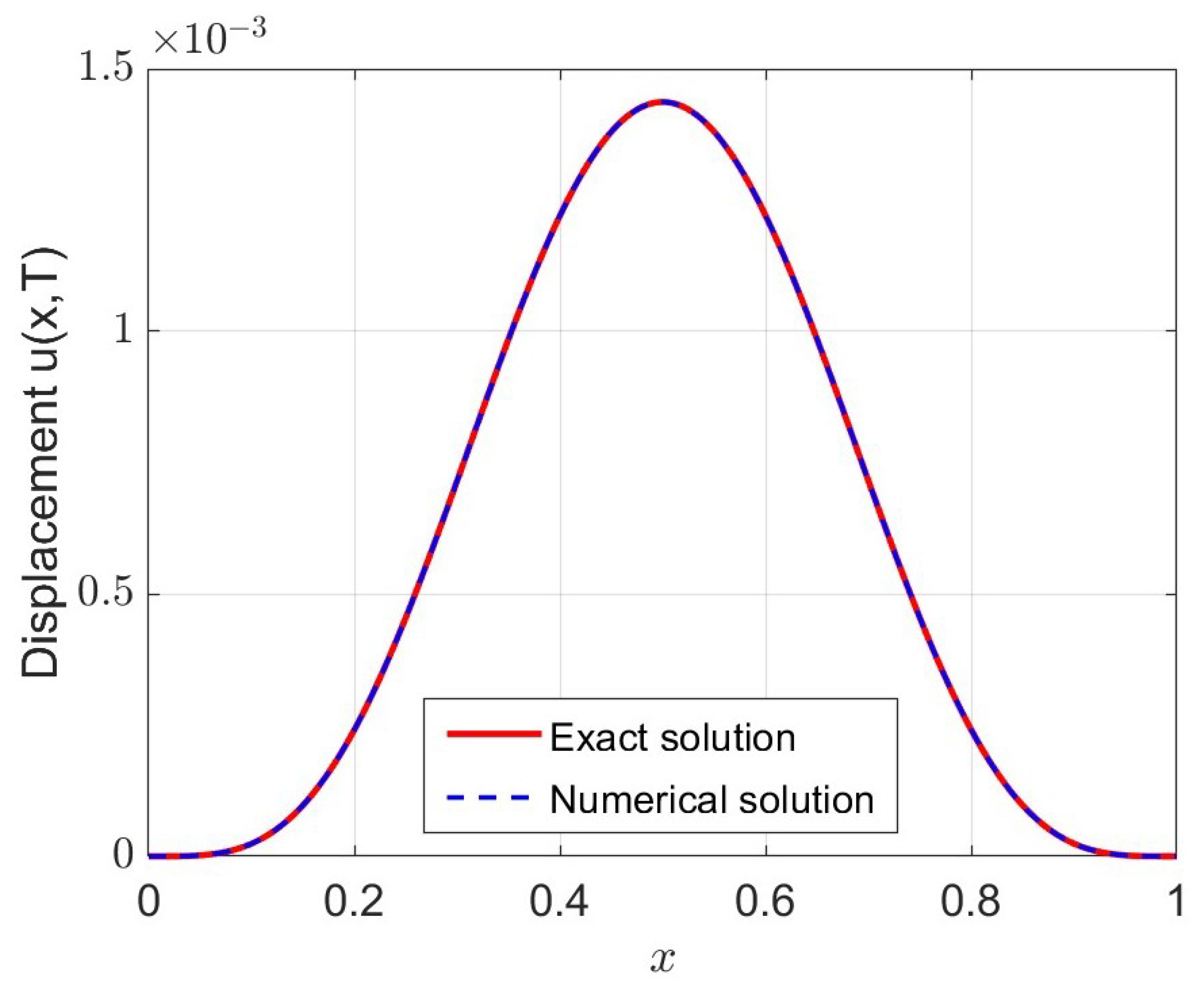
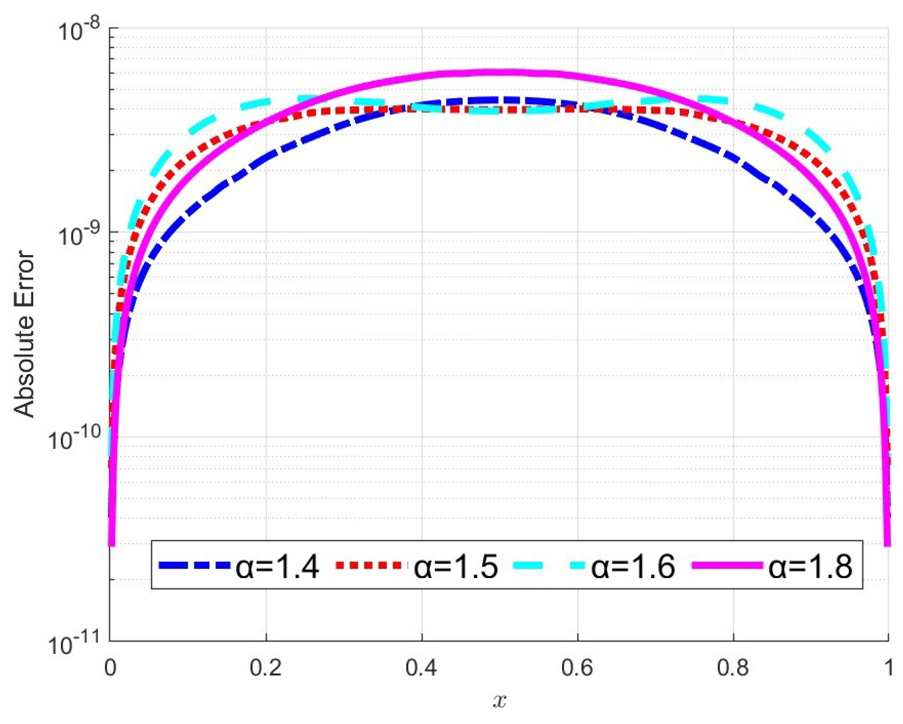
5.1. Convergence Rate

To verify the convergence rate, consider the equation

$${\displaystyle \frac{{\partial }^{2}u(x,t)}{\partial t^2}}+{(-\Delta )}^{\alpha /2}u(x,t)+\gamma {\displaystyle \frac{\partial u(x,t)}{\partial t}}+sin\left(u\right)=f(x,t),x\in (0,1),t\in (0,1],$$

(33)

with the forcing function defined as

$$\begin{array}{cc}\hfill f(x,t)=& sin(x^4{(1-x)}^{4}exp(-t))+(1-\gamma ){(1-x)}^4{x}^{4}exp(-t)\hfill \\ & +{\displaystyle \frac{exp(-t)}{2cos(\alpha \pi /2)}}[{\displaystyle \frac{\Gamma \left(5\right)(x^{4-\alpha }+{(1-x)}^{4-\alpha })}{\Gamma (5-\alpha )}}\hfill \\ & -{\displaystyle \frac{4\Gamma \left(6\right)({(1-x)}^{5-\alpha }+x^{5-\alpha })}{\Gamma (6-\alpha )}}+{\displaystyle \frac{6\Gamma \left(7\right)({(1-x)}^{6-\alpha }+x^{6-\alpha })}{\Gamma (7-\alpha )}}\hfill \\ & -{\displaystyle \frac{4\Gamma \left(8\right)(x^{7-\alpha }+{(1-x)}^{7-\alpha })}{\Gamma (8-\alpha )}}+{\displaystyle \frac{\Gamma \left(9\right)({(1-x)}^{8-\alpha }+x^{8-\alpha })}{\Gamma (9-\alpha )}}].\hfill \end{array}$$

Initial and boundary conditions are given as

$$\begin{array}{cc}\hfill & u(x,0)=x^4{(1-x)}^4,{\displaystyle \frac{\partial u(x,0)}{\partial t}}=-x^4{(1-x)}^4,0\le x\le 1,\hfill \\ \hfill & u(0,t)=u(1,t)=0,t>0.\hfill \end{array}$$

Problem (33) admits an exact solution under the specified constraints, expressed explicitly as

$$u(x,t)=exp(-t){(1-x)}^4{x}^4.$$

Let $e(h,\tau )$ represent the computational error associated with spatial step h and temporal step $\tau$ at time $t=T$ in the $L^2$-norm, calculated by

$$e(h,\tau )=\sqrt{h\sum _{i=1}^{N_x-1}{|u(x_i,T)-u_i^{N_t}|}^2}.$$

To quantify convergence behavior, the experimental order of convergence (EOC) is calculated through

$$EOC={log}_2{\displaystyle \frac{e(h,\tau )}{e(h/2,\tau /2)}}.$$

Table 1. The errors and EOC of the numerical method given in (16) and (17) together with the initial value scheme in (21) (Present method) compared with the EGL method for Equation (33) with $\alpha =1.2,1.5,1.8$ by keeping $h=\tau$ at time $T=1$.

$\mathit{\gamma }$	$\mathit{h}=\mathit{\tau }$	$\mathit{\alpha }=1.2$				$\mathit{\alpha }=1.5$				$\mathit{\alpha }=1.8$
		Present		EGL		Present		EGL		Present		EGL
		$\mathit{e}(\mathit{h},\mathit{\tau })$	EOC	$\mathit{e}(\mathit{h},\mathit{\tau })$	EOC	$\mathit{e}(\mathit{h},\mathit{\tau })$	EOC	$\mathit{e}(\mathit{h},\mathit{\tau })$	EOC	$\mathit{e}(\mathit{h},\mathit{\tau })$	EOC	$\mathit{e}(\mathit{h},\mathit{\tau })$	EOC
0	1/32	$3.66\times {10}^{-7}$	–	$5.89\times {10}^{-3}$	–	$1.28\times {10}^{-6}$	–	$4.98\times {10}^{-3}$	–	$2.43\times {10}^{-6}$	–	$5.56\times {10}^{-3}$	–
	1/64	$1.63\times {10}^{-7}$	1.17	$3.16\times {10}^{-3}$	0.90	$2.70\times {10}^{-7}$	2.24	$2.58\times {10}^{-3}$	0.95	$4.14\times {10}^{-7}$	2.55	$2.83\times {10}^{-3}$	0.98
	1/128	$4.37\times {10}^{-8}$	1.90	$1.75\times {10}^{-3}$	0.85	$5.78\times {10}^{-8}$	2.22	$1.42\times {10}^{-3}$	0.86	$7.83\times {10}^{-8}$	2.40	$1.59\times {10}^{-3}$	0.84
	1/256	$1.12\times {10}^{-8}$	1.97	$1.15\times {10}^{-3}$	0.61	$1.37\times {10}^{-8}$	2.08	$9.76\times {10}^{-4}$	0.54	$1.75\times {10}^{-8}$	2.16	$1.01\times {10}^{-3}$	0.66
	1/512	$2.81\times {10}^{-9}$	1.99	$6.95\times {10}^{-4}$	0.72	$3.37\times {10}^{-9}$	2.02	$6.09\times {10}^{-4}$	0.68	$4.25\times {10}^{-9}$	2.05	$5.98\times {10}^{-4}$	0.75
0.5	1/32	$2.88\times {10}^{-7}$	–	$6.23\times {10}^{-3}$	–	$1.04\times {10}^{-6}$	–	$5.10\times {10}^{-3}$	–	$2.11\times {10}^{-6}$	–	$7.57\times {10}^{-3}$	–
	1/64	$1.33\times {10}^{-7}$	1.87	$4.36\times {10}^{-3}$	0.52	$2.26\times {10}^{-7}$	2.21	$4.00\times {10}^{-3}$	0.35	$3.56\times {10}^{-7}$	2.57	$5.67\times {10}^{-3}$	0.42
	1/128	$3.64\times {10}^{-8}$	1.87	$2.86\times {10}^{-3}$	0.61	$4.81\times {10}^{-8}$	2.23	$2.50\times {10}^{-3}$	0.68	$6.69\times {10}^{-8}$	2.41	$3.66\times {10}^{-3}$	0.63
	1/256	$9.37\times {10}^{-9}$	1.96	$2.01\times {10}^{-3}$	0.51	$1.13\times {10}^{-8}$	2.09	$1.80\times {10}^{-3}$	0.47	$1.50\times {10}^{-8}$	2.16	$2.56\times {10}^{-3}$	0.52
	1/512	$2.36\times {10}^{-9}$	1.99	$1.15\times {10}^{-3}$	0.81	$2.78\times {10}^{-9}$	2.02	$1.05\times {10}^{-3}$	0.78	$3.62\times {10}^{-9}$	2.05	$1.47\times {10}^{-3}$	0.80

shows the error and EOC of the numerical method (16) and (17) and the initial value scheme (21) for Equation (33) by keeping $h=\tau$ at time $T=1$ when the values of $\alpha$ and h are different.

The numerical results in Table 1 show that the present numerical method has second-order accuracy both in the spatial and temporal directions for different $\alpha$ and $\gamma$. For this example, the function is smooth enough, so it achieves second-order convergence to the fractional Laplacian. When a function exhibits singularity along the boundary, the convergence order is anticipated to drop below two. Nevertheless, our numerical examples reveal that the approximation maintains second-order convergence in the interior domain.

In Figure 1, we show a comparison between the exact solution and the numerical solution of Equation (33) obtained by the proposed numerical method with $h=\tau =1/512$. Figure 2 shows the absolute error with different $\alpha$ values. The numerical results presented in Figure 1 and Figure 2 demonstrate the effectiveness of the proposed numerical method. The results show a second-order temporal discretization with a high-order spatial approximation for the fractional Laplacian, achieving second-order convergence in both time and space, and the errors decrease optimally as $h=\tau$ is refined. For comparison purposes, we reduce the NSFSGE to a problem involving a first-order-derivative system and subsequently employe a first-order Euler method combined with a Grünwald–Letnikov approximation for the space fractional derivatives; we denote this method the EGL method. This approach is straightforward but theoretically limited to first-order accuracy in time and the first or second order in space [30].

The proposed method exhibits significantly smaller errors compared to the EGL method for the same step size $h=\tau$. The errors of the present method can reach ${10}^{-8}$, whereas the EGL method only achieves ${10}^{-4}$. Additionally, the proposed method maintains an EOC close to 2, confirming its second-order convergence, while the EGL method exhibits an EOC approaching one. This discrepancy primarily stems from the use of the first-order Euler method in the temporal direction. It should be noted that second-order or higher-order temporal methods have already been studied; we merely employ this example for error comparison purposes here.

5.2. Energy Dissipation or Conservation

In this part, we verify the energy conservation or dissipation behavior of the present method by considering the NSFSGE (3) with $\beta =0$ in the domain $x\in [-40,40]$, $t\in (0,T]$ and the initial conditions

$$u(x,0)=4arctan\left({\displaystyle \frac{\sqrt{1-w^2}}{wcosh\sqrt{1-w^2}}}\right),{\displaystyle \frac{\partial u(x,0)}{\partial t}}=0,$$

where $0<w<1$.

In Figure 3, the surface plot of the numerical solution $u^n$ for the NSFSGE (3) with $w=0.85$ and $\gamma =0$, which is computed using the present method with spatial step $h=1/4$ and temporal step $\tau =1/16$, is given in the left subplot, and the right subplot shows the discrete energy $E_n$ defined by (23) with different parameters $\alpha$ and $\epsilon$. It can be seen that the proposed scheme exhibits inherent energy conservation characteristics under $\gamma =0$. For different values of $\epsilon$, the range of numerical solutions changes from $[-2,2]$ when $\epsilon =1$ to $[-5,5]$ when $\epsilon =0.5$. Additionally, Figure 3 clearly reveals the influence of different values of $\alpha$ on the surface of the numerical solution, while the numerical method is verified to be suitable for long-time simulations in this example.

For $\gamma >0$, the system governed by (3) is energy dissipative. Figure 4 presents surface visualizations in its left-hand panels and the temporal evolution of the discrete energy $E_n$ in its right-hand panels of the corresponding numerical solutions with different values of $\gamma$ and $\alpha$ obtained by using the proposed method with $h=1/4$ and $\tau =1/32$.

Figure 4 demonstrates that the proposed numerical method conserves the energy-dissipation principle of (3) under $\gamma >0$, which validates the theoretical conclusion established in Theorem 2. Moreover, Figure 4 further illustrates that the solution surfaces change corresponding to varying $\gamma$ values, and the amplitude of the solutions decreases as $\gamma$ decreases, and the lower $\gamma$ values significantly attenuated discrete energy variation rates.

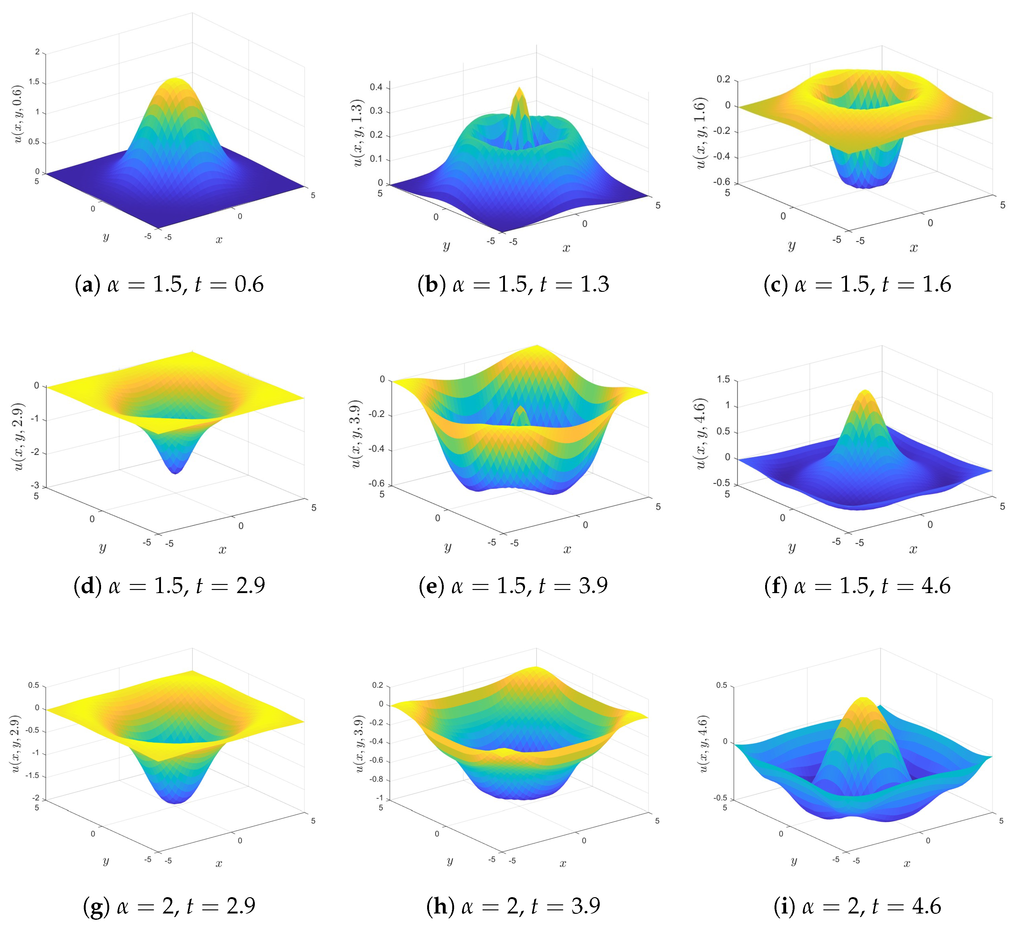
5.3. Two-Dimensional Problem

Consider the following two-dimensional sine-Gordon problem:

$${\displaystyle \frac{{\partial }^{2}u(\mathbf{x},t)}{\partial t^2}}+{(-\Delta )}^{\alpha /2}u(\mathbf{x},t)+\gamma {\displaystyle \frac{\partial u(\mathbf{x},t)}{\partial t}}+{\displaystyle \frac{1}{\epsilon }}sin\left(\epsilon u(\mathbf{x},t)\right)=0,$$

(34)

where $\mathbf{x}=(x, y)$ is the two-dimensional space on the finite domain $\Omega =B\times (0, T]$ with $B=(a_1, b_1)\times (a_2, b_2)$. Define the mesh point $x_i=a_1+i{h}_x$, with $i=1,2,\dots ,N_x-1$, and let $y_j=a_2+j{h}_y$, $j=1,2,\dots ,N_y-1$ with $h_x=(b_1-a_1)/N_x$, $h_y=(b_2-a_2)/N_y$. Consequently, the method proposed in this paper for the one-dimensional case can be extended to the two-dimensional case directly. All essential features presented for the one-dimensional Equation (3) can also be extended to the two-dimensional case.

Specifically, in this example, we consider the two-dimensional Equation (34) subjected to the initial conditions

$$u_0(x,y,0)={\displaystyle \frac{2}{cosh\left[0.3(x^2+y^2)\right]}},u_1(x,y,0)=0,$$

for $(x, y)\in \overline{B}$ and the Dirichlet boundary condition $u(x, y, t)=0$ for $(x, y)\in \partial B$ with $B=(-5, 5)\times (-5, 5)$, $\alpha =1.5$, $\gamma =0$, and $\epsilon =1$. We discretize the spatial fractional Laplacian by using the discrete fractional Laplacian operator with step sizes $h_x=h_y=h=0.25$ and $\tau =0.01$. In Figure 5, we present the numerical solutions and the corresponding contour plots of Equation (34) with $\alpha =1.5$ and $\alpha =2$ at the time points $t=0.6, 1.3, 1.6, 2.9, 3.9$, and $4.6$. The solutions appear to follow almost a periodic behavior.

Figure 5 illustrates the numerical solution of the structure-preserving finite difference scheme for the nonlinear space fractional sine-Gordon equation with damping based on the T-SAV approach (34), exhibiting characteristic breather solution behavior. The solution demonstrates significant periodic amplitude modulation within the spatial domain $B=(-5, 5)\times (-5, 5)$. Persistent energy localization occurs in the core region, where the amplitude evolves through quasi-periodic expansion–contraction cycles, consistent with fundamental breather characteristics. At the same time, the classical breather solutions of Equation (34) with $\alpha =2$ at $t=2.9$, $3.9$, and $4.6$ are also shown in Figure 5. Compared with the corresponding results in the fractional-order case in Figure 5, it can be seen that the boundary of the classical breathers has almost no oscillation, while the boundary of the fractional-order case still has obvious oscillations, indicating a slower spatial decay. Additionally, both the waveform and peak values of the breathers at the same time points are different between the classical and fractional-order cases.

6. Conclusions

In this paper, the NSFDGE with a damping term is transformed into a structure-preserving equivalent system satisfying the modified energy conservation or dissipation law by using the T-SAV method. By combining a second-order central difference method and the finite difference method, the numerical method obtains the optimal convergence rate of $\mathrm{O}({\tau }^2+h^{\delta })$ while strictly maintaining the discrete energy dissipation/conservation law. The boundedness and convergence of the numerical solution are proved by theoretical analysis. Numerical experiments confirm the effictiveness of the numerical method for different fractional orders $\alpha$, damping terms $\gamma$, and nonlinear strengths $\epsilon$, and prove the long-term simulation ability of the numerical scheme to simulate nonlinear wave phenomena. Although the current scheme effectively handles one- and two-dimensional problems, extending the method to higher-dimensional fractional wave systems in the future research will broaden its applicability to complex physical systems, such as quantum field theory and turbulence. Moreover, extending the proposed method to a variable-step format would significantly enhance the computational efficiency of long-term estimation.

References

1. Kilbas, A.A.; Srivastava, H.M.; Trujillo, J.J. Theory and Applications of Fractional Differential Equations; Elsevier: Amsterdam, The Netherlands, 2006. [Google Scholar]
2. Baleanu, D.; Diethelm, K.; Scalas, E.; Trujillo, J.J. Fractional Calculus: Models and Numerical Methods; Springer: Berlin/Heidelberg, Germany, 2012. [Google Scholar]
3. Gu, X.M.; Zhao, Y.L.; Zhao, X.L.; Carpentieri, B.; Huang, Y.Y. A note on parallel preconditioning for the all-at-once solution of Riesz fractional diffusion equations. Numer. Math. Theory Methods Appl. 2021, 14, 1003–1026. [Google Scholar] [CrossRef]
4. Zhao, J.J.; Jiang, X.Z.; Xu, Y. A kind of generalized backward differentiation formulae for solving fractional differential equations. Appl. Math. Comput. 2022, 419, 126872. [Google Scholar] [CrossRef]
5. Fu, Y.Y.; Cai, W.J.; Wang, Y.S. A linearly implicit structure-preserving scheme for the fractional Sine-Gordon equation based on the IEQ approach. Appl. Math. Comput. 2021, 404, 126281. [Google Scholar] [CrossRef]
6. Korabel, N.; Zaslavsky, G.M.; Tarasov, V.E. Coupled oscillators with power-law interaction and their fractional dynamics analogues. Commun. Nonlinear Sci. Numer. Simul. 2007, 12, 1003–1017. [Google Scholar] [CrossRef]
7. Macías-Díaz, J.E. Numerical study of the process of nonlinear supratransmission in Riesz space-fractional Sine-Gordon equations. Commun. Nonlinear Sci. Numer. Simul. 2017, 46, 89–102. [Google Scholar] [CrossRef]
8. Amabili, M.; Balasubramanian, P.; Ferrari, G. Nonlinear vibrations and damping of fractional viscoelastic rectangular plates. Nonlinear Dyn. 2021, 103, 1–29. [Google Scholar] [CrossRef]
9. Jia, J.H.; Zheng, X.C.; Wang, H. Numerical discretization and fast approximation of a variably distributed-order fractional wave equation. ESAIM. Math. Model. Numer. Anal. 2021, 55, 2211–2232. [Google Scholar] [CrossRef]
10. Tarasov, V.E.; Aifantis, E.C. Non-standard extensions of gradient elasticity: Fractional non-locality, memory and fractality. Int. J. Eng. Sci. 2014, 83, 1–22. [Google Scholar] [CrossRef]
11. Huang, Y.; Oberman, A. Numerical methods for the fractional Laplacian: A finite difference-quadrature approach. SIAM J. Numer. Anal. 2014, 52, 3056–3084. [Google Scholar] [CrossRef]
12. Lischke, A.; Pang, G.F.; Gulian, M.; Song, F.Y.; Glusa, C.; Zheng, X.N.; Mao, Z.P.; Cai, W.; Meerschaert, M.M.; Ainsworth, M. What is the fractional Laplacian? A comparative review with new results. J. Comput. Phys. 2019, 404, 109023. [Google Scholar] [CrossRef]
13. Jia, J.; Jiang, X.; Chi, X. Improved uniform error bounds of Lawson-type exponential integrator method for long-time dynamics of the high-dimensional space fractional Sine-Gordon equation. Numer. Algorithms 2024, 97, 1179–1214. [Google Scholar] [CrossRef]
14. Hu, D.D.; Cai, W.J.; Xu, Z.Z.; Bo, Y.H.; Wang, Y.S. Dissipation-preserving Fourier pseudo-spectral method for the space fractional nonlinear Sine-Gordon equation with damping. Math. Comput. Simul. 2021, 188, 1–18. [Google Scholar] [CrossRef]
15. Nikan, O.; Avazzadeh, Z.; Machado, J.A.T. Numerical investigation of fractional nonlinear sine-Gordon and Klein-Gordon models arising in relativistic quantum mechanics. Eng. Anal. Bound. Elem. 2020, 120, 223–237. [Google Scholar] [CrossRef]
16. Ran, M.; Zhang, C. Compact difference scheme for a class of fractional-in-space nonlinear damped wave equations in two space dimensions. Comput. Math. Appl. 2016, 71, 1151–1162. [Google Scholar] [CrossRef]
17. Alfimov, G.; Pierantozzi, T.; Vázquez, L. Numerical study of a fractional Sine-Gordon equation. J. Phys. A Math. Gen. 2004, 37, 10767–10781. [Google Scholar] [CrossRef]
18. Mirzaei, D.; Dehghan, M. Boundary element solution of the two-dimensional Sine-Gordon equation using continuous linear elements. Eng. Anal. Bound. Elem. 2009, 33, 12–24. [Google Scholar] [CrossRef]
19. Achouri, T.; Simos, T.E. Conservative finite difference scheme for the nonlinear fourth-order wave equation. Appl. Math. Comput. 2019, 359, 121–131. [Google Scholar] [CrossRef]
20. Tlili, K. On the L-convergence of two conservative finite difference schemes for fourth-order nonlinear strain wave equations. Comput. Appl. Math. 2021, 40, 1–31. [Google Scholar] [CrossRef]
21. Yang, J.X.; Kim, J. The stabilized-trigonometric scalar auxiliary variable approach for gradient flows and its efficient schemes. J. Eng. Math. 2021, 129, 1–26. [Google Scholar] [CrossRef]
22. Shen, J.; Xu, J. Convergence and error analysis for the scalar auxiliary variable schemes to gradient flows. SIAM J. Numer. Anal. 2018, 56, 2895–2912. [Google Scholar] [CrossRef]
23. Hou, D.M.; Azaiez, M.; Xu, C.J. A variant of scalar auxiliary variable approaches for gradient flows. J. Comput. Phys. 2019, 395, 26. [Google Scholar] [CrossRef]
24. Shen, J.; Xu, J.; Yang, J. A new class of efficient and robust energy stable schemes for gradient flows. J. Sci. Comput. 2017, 73, 218–245. [Google Scholar] [CrossRef]
25. Fu, Y.Y.; Hu, D.D.; Wang, Y.S. High-order structure-preserving algorithms for the multi-dimensional fractional nonlinear Schrödinger equation based on the SAV approach. Math. Comput. Simul. 2021, 185, 1–20. [Google Scholar] [CrossRef]
26. Fu, Y.Y.; Cai, W.J.; Wang, Y.S. A structure-preserving algorithm for the fractional nonlinear Schrödinger equation based on the SAV approach. Commun. Nonlinear Sci. Numer. Simul. 2019, 72, 105–121. [Google Scholar] [CrossRef]
27. Hao, Z.; Zhang, Z.; Du, R. Fractional centered difference scheme for high-dimensional integral fractional Laplacian. J. Comput. Phys. 2021, 424, 109851. [Google Scholar] [CrossRef]
28. Hu, D.; Cai, W.; Fu, Y.; Wang, Y. Fast dissipation-preserving difference scheme for nonlinear generalized wave equations with the integral fractional Laplacian. Commun. Nonlinear Sci. Numer. Simul. 2021, 99, 105786. [Google Scholar] [CrossRef]
29. Tian, Z.H.; Ran, M.H.; Liu, Y. Higher-order energy-preserving difference scheme for the fourth-order nonlinear strain wave equation. Comput. Math. Appl. 2023, 128, 221–235. [Google Scholar] [CrossRef]
30. Scherer, R.; Kalla, S.L.; Tang, Y.; Huang, J. The Grunwald-Letnikov method for fractional differential equations. Comput. Math. Appl. 2011, 62, 902–917. [Google Scholar] [CrossRef]
Figure 1. Comparison between the numerical solution and the exact solution.
Fractalfract 09 00455 g001
Figure 2. Absolute error for different α .
Fractalfract 09 00455 g002
Figure 3. The surface of the numerical solution and the discrete energy E n for γ = 0 , and different values of α and ε .
Fractalfract 09 00455 g003
Figure 4. The surface of the numerical solution and the discrete energy E n with ε = 1 , for different γ and α , obtained using the present method with h = 1 / 4 and τ = 1 / 32 .
Fractalfract 09 00455 g004
Figure 5. The surface of the numerical solution of Equation (34) versus the spatial coordinates x and y in the spatial domain B = ( 5 , 5 ) × ( 5 , 5 ) R 2 with γ = 0 and different α at various times t = 0.6 , 1.3 , 1.6 , 2.9 , 3.9 , 4.6 by using the present method.
Fractalfract 09 00455 g005