Multifractal-Aware Convolutional Attention Synergistic Network for Carbon Market Price Forecasting

Abstract

Accurate carbon market price prediction is crucial for promoting a low-carbon economy and sustainable engineering. Traditional models often face challenges in effectively capturing the multifractality inherent in carbon market prices. Inspired by the self-similarity and scale invariance inherent in fractal structures, this study proposes a novel multifractal-aware model, MF-Transformer-DEC, for carbon market price prediction. The multi-scale convolution (MSC) module employs multi-layer dilated convolutions constrained by shared convolution kernel weights to construct a scale-invariant convolutional network. By projecting and reconstructing time series data within a multi-scale fractal space, MSC enhances the model’s ability to adapt to complex nonlinear fluctuations while significantly suppressing noise interference. The fractal attention (FA) module calculates similarity matrices within a multi-scale feature space through multi-head attention, adaptively integrating multifractal market dynamics and implicit associations. The dynamic error correction (DEC) module models error commonality through variational autoencoder (VAE), and uncertainty-guided dynamic weighting achieves robust error correction. The proposed model achieved an average R² of 0.9777 and 0.9942 for 7-step ahead predictions on the Shanghai and Guangdong carbon price datasets, respectively. This study pioneers the interdisciplinary integration of fractal theory and artificial intelligence methods for complex engineering analysis, enhancing the accuracy of carbon market price prediction. The proposed technical pathway of “multi-scale deconstruction and similarity mining” offers a valuable reference for AI-driven fractal modeling.

1. Introduction

Transitioning to low-carbon energy is a pivotal strategy to optimize energy consumption structures and promote sustainable development. Carbon emissions trading systems and carbon tax policies are widely recognized as key points for a low-carbon economy [1]. The formation of a carbon market price that meets the supply and demand mechanisms according to the current market situation is the core of the carbon trading market [2]. Therefore, accurate prediction of carbon market price is the core requirement for carbon market participants to optimise their decision-making, and it is also the key technical support to achieve the goal of ‘dual-carbon’ strategy and the transformation of a low-carbon economy [3]. However, the carbon market price time series in China exhibits characteristics similar to those of financial time series, including overall volatility, heavy tails, and non-normal distribution [4]. Its high nonlinearity and non-stationarity lead to complex price fluctuations, posing significant challenges for accurate carbon price prediction.

Fractal theory has been widely applied in the modeling and structural analysis of complex systems. In financial markets, it is often used to analyze asymmetric and volatile market behaviors, aiding in the identification of nonlinearity and long-memory characteristics in financial time series. Additionally, in tasks such as large language models and image processing, fractal theory is commonly employed to jointly analyze local data and global trends, quantify the self-similarity of language, and perform fractal-based data augmentation. Fractal theory provides theoretical support for understanding complex structures and developing multi-scale analysis algorithms. However, traditional fractal models primarily rely on statistical measures to reveal the nonlinear characteristics, long-memory effects, and scale-invariant structures in multifractal complex systems. Fan et al. [5] used multifractal detrended volatility analysis (MFDFA) to calculate the generalised Hurst exponent h(q), which breaks through the limitations of the qualitative study of the traditional efficient market hypothesis (EMH) and proves the multifractal nature of the carbon market time series. Khurshid et al. [6] applied methods such as Asymmetric Multifractal Detrended Fluctuation Analysis (A-MFDFA) to examine the asymmetric multifractal characteristics and market efficiency of global and Chinese green energy markets. Their study captured the asymmetric multifractal features of price uptrends and downtrends, and constructed a Market Inefficiency Index (MLM) by integrating the Market Deficiency Measure (MDM) and the Hurst exponent, offering a comparative analysis of market dynamics before and after the COVID-19 pandemic. Li and Tian [7] combined the BEAST algorithm with Skewed Multifractal Detrended Cross-Correlation Analysis (MF-DCCA) to detect structural breakpoints in carbon market time series. Their research addressed the limitations of traditional multifractal analysis by accounting for the impact of abrupt changes on the cross-correlation between carbon price and trading volume, and tackled the lack of dynamic efficiency evaluation under pandemic-induced shocks. Ni et al. [8] proposed a stock trend prediction model based on fractal feature selection and Support Vector Machines (SVM). The model measured feature importance using fractal dimensions and employed an Ant Colony Optimization algorithm to select optimal feature subsets, effectively overcoming the limitations of conventional feature selection methods in determining the optimal number of features and handling nonlinear relationships. Liu & Huang et al. [9] use Fractal Brownian Motion (FBM) to effectively portray the long memory and fractal characteristics of the time series, and describe the time-varying volatility of the financial time series through the Generalised Autoregressive Conditional Heteroskedasticity (GARCH) model, which can better adapt to the changes in market structure. Raubitzek and Neubauer [10] proposed a method that integrates fractal interpolation with Long Short-Term Memory (LSTM) neural networks. By using fractal interpolation to dynamically adapt to the complexity characteristics of time series—such as the Hurst exponent—they generated finer-grained sequences that better match the complexity of real-world systems. This approach addresses the poor predictive performance of conventional LSTM models when dealing with insufficient data or highly complex structures. Dandan et al. [11] introduced the Skewed-t distribution—capable of capturing the leptokurtic and skewed features of return series—into the Markov-switching multifractal (MSM) model, forming the Skewed-t-MSM-EVT model to quantify extreme risks in the carbon market. This model overcomes the limitations of traditional approaches that fail to fully account for the multifractal properties of carbon markets and the asymmetry in return distributions. Jin et al. [12] developed a short-term wind speed prediction model that integrates Fractal Dimension (FD), Variational Mode Decomposition (VMD), and Generalized Continued Fraction (GCF). By determining VMD decomposition parameters based on the fractal characteristics of wind speed series, the model solves the ambiguity in parameter selection faced by traditional VMD methods and enhances the ability to capture dynamic wind speed patterns. Alabdulmohsin et al. [13] employed an information-theoretic approach to convert text into bit sequences and used fractal theory to quantify the self-similarity and long-range dependencies of language. This method addresses the incomplete characterization of linguistic structures caused by computational constraints in previous studies, offering a novel perspective for understanding the nature of language and the success of large language models (LLMs). However, traditional econometric models need to go through multiple steps such as distributional assumptions, parameter estimation, and cointegration tests, which makes the modeling process complicated and sensitive to pre-processing. Moreover, traditional econometric models are difficult to capture the nonlinear characteristics and non-stationarity of the carbon market price series due to stringent assumptions [14], and the prediction error is significantly enlarged, especially in the face of sudden market changes. For complex systems, the calculation results of econometric methods are often not intuitive, requiring in-depth research and professional analysis, and the results are difficult to understand and apply.

Deep learning models support end-to-end modeling without manual feature engineering, with powerful nonlinear mapping capability, and support online updating and migration. CNN and its many variants have been widely used in carbon market price time series feature extraction due to their feature extraction advantages, such as parallel computing and local awareness. Transformer, with its core of self-attention mechanism, can effectively capture long-distance dependencies and complex nonlinear features, and has been widely used this year. Wu et al. [15] integrated four different kernels of 1D convolution as a multi-scale extraction module and improved the feature learning ability by designing a dual-stream Transformer module to capture multivariate internal relations and univariate time dependence, respectively. Yin et al. [16] proposed a spatio-temporal multi-dimensional collaborative attention network (TSMA) that, through the temporal attention mechanism, feature attention mechanism, and convolutional block attention module, the features of multi-region information at different spatio-temporal levels are fully extracted, and BIGRU further extracts the time series features and predicts them. Ji et al. [17] (2025) proposed the QRTransformer-MIDAS model, which integrates quantile regression, Transformer architecture, and mixed-frequency modeling. By employing Mixed Data Sampling (MIDAS) regression, the model captures the influence of high-frequency variables on low-frequency carbon prices. It leverages the transformer to model nonlinear dependencies and utilizes kernel density estimation (KDE) for probabilistic forecasting. This approach addresses key limitations of traditional same-frequency models, such as neglecting high-frequency information and relying solely on point forecasts that fail to capture uncertainty in volatility. Zhang et al. [18] implemented a framework that performs multi-scale decomposition and reconstruction of carbon price series via adaptive feature extraction and entropy-based recomposition. The method expands the model’s local receptive field through time series patching and applies a two-stage stabilization process to enhance adaptability to non-stationary data. Additionally, a dynamic weighted ensemble algorithm is designed to intelligently assign weights to sub-sequences, overcoming limitations of traditional models related to insufficient feature extraction and sub-sequence weight misallocation.

Due to the multi-scale complexity characteristics of carbon market price time series data, multi-scale decomposition methods are often combined with deep learning methods, which can reduce the data complexity to improve the prediction performance. Current carbon market price prediction models mostly use signal processing methods for multi-scale decomposition. Yue et al. [19] used the Hampel identifier (HI) for outlier processing, time-varying filtering empirical modal decomposition (TVFEMD) for data decomposition and reconstruction, and the Transformer model for multi-step ahead and interval prediction of carbon market price to cope with the nonlinearities, nonsmoothness, and complex fluctuations of the carbon market price series. Smoothness and complex fluctuation problems. Hong et al. [20] proposed a hybrid model combining depth-enhanced frequency-enhanced decomposition transformer (DA-FEDformer), improved complete ensemble empirical modal decomposition with adaptive noise (ICEEMDAN) and multi-model optimised segmentation error correction, which organically integrates the frequency and time domain information and improves the performance of carbon market price prediction. Sun et al. [21] used discrete wavelet transform (DWT), complete ensemble empirical modal decomposition of adaptive noise (CEEMDAN) and singular spectrum analysis (SSA) for hybrid multi-scale decomposition and Transformer model for prediction, which improves the model’s fitting and prediction of the data by utilising the carbon market price prediction model with multi-source information and specific data processing methods. Li et al. [22] proposed a dual decomposition ensemble model based on the Sparrow Search Algorithm-optimized Variational Mode Decomposition (SVMD). The model classifies decomposed components using fuzzy entropy, then applies Whale Optimization-enhanced LSTM and Extreme Learning Machine (ELM) for prediction, respectively. Additionally, it introduces Ensemble Empirical Mode Decomposition (EEMD) to further decompose and correct residual error sequences. This approach overcomes issues such as mode mixing and parameter dependency commonly found in traditional decomposition methods. Liu et al. [23] addressed mixed-frequency data by applying frequency alignment and implementing a sub-model selection strategy to match different feature sub-sequences. A multi-objective optimization algorithm is then used to determine integration weights. This method resolves limitations in conventional models that overlook the influence of high-frequency external variables, lack adaptability in sub-sequence model matching, and inadequately optimize ensemble weights. Cai et al. [24] employed the adaptive white-noise-assisted Complete Ensemble Empirical Mode Decomposition with Adaptive Noise (CEEMDAN) to decompose nonlinear and non-stationary carbon price series into structured components such as high-frequency, low-frequency, and trend residuals. Temporal features of each component are then extracted using a TCN-LSTM model to achieve accurate predictions. This approach addresses challenges in capturing complex carbon price fluctuations and reduces the vulnerability of single deep learning models to noise interference. Ma et al. [25] proposed the TCN-LSTM-Self-Attention model for carbon price prediction, which integrates decomposition and a dual-channel attention mechanism. The Temporal Convolutional Network (TCN) is used to extract short-term local features, the LSTM captures long-term dependencies, and self-attention is introduced to enhance the importance of key information. This model effectively overcomes the limitation of traditional methods in jointly modeling short-term volatility and long-term trends. Lu et al. [26] transformed the maximum and minimum carbon prices into central and radius sequences to capture volatility information. Variational Mode Decomposition parameters are optimized using a Differential Evolution Algorithm, and fuzzy entropy is used to reconstruct subsequences. Optimal Multi-Kernel Support Vector Regression (MKSVR) and Exponential Generalized Autoregressive Conditional Heteroskedasticity (EGARCH) models are applied to different sub-sequence types. This method addresses deficiencies in handling interval data volatility, subjective parameter selection in decomposition, and poor adaptability of single kernel functions. Fang et al. [27] developed a carbon price prediction model based on secondary decomposition and BiLSTM. It uses CEEMDAN and VMD to perform a two-stage decomposition of carbon price time series and adopts the Capuchin Optimization Algorithm (COA) to fine-tune BiLSTM parameters such as step size and number of neurons. This framework enables deep feature extraction and model parameter optimization for complex carbon price sequences. Dong et al. [28] employs a multi-wavelet-layered stacked DWNN (Deep Wavelet Neural Network) to achieve more accurate approximation of nonlinear mappings through multi-scale feature extraction.

However, there are still three limitations of existing carbon market price forecasting models.

(1)

Most of the existing fractal models are based on traditional statistics and machine learning methods, which struggle to deeply explore multiple fractal characteristics and make predictions. For complex systems, the calculation results of econometric statistical methods are often not intuitive, requiring in-depth research and professional analysis, and the results are difficult to understand and apply practically in prediction tasks. The combination of deep learning models and fractal theory is insufficient, and there is a lack of integration of interdisciplinary methods.

(2)

Most of the existing multi-scale prediction methods for carbon market price are based on signal processing, using a fixed way of decomposition, are difficult to co-optimize with downstream models, and lack end-to-end learning, dynamic adaptation, and complex feature modeling capabilities.

(3)

Existing forecasting frameworks are difficult to model complex dynamic changes in time series and multiple fractalities well, and there are problems such as gradient disappearance or gradient explosion.

Considering the aforementioned drawbacks and the improvement of carbon market price prediction, this study designs the MF-Transformer-DEC model that contains a multi-scale convolution module, a fractal attention module, and a dynamic error correction module. In addition, to illustrate the superiority of the proposed model, we evaluate it through several experiments. The main contributions of this research are as follows.

(1) A novel multi-scale similarity modeling method MF-Transformer-DEC, is proposed, integrating the self-similarity and scale invariance theories of fractals to build a robust prediction framework with strong feature modeling and mining capabilities. The understanding and prediction ability of complex systems are enhanced.

(2) The multifractal-driven multi-scale convolution (MSC) module introduces a scale-invariant convolutional network, which projects and reconstructs time series data within a multi-scale fractal space, thereby enhancing the model’s ability to comprehend multi-scale chaotic sequences. By assigning distinct dilation rates to each convolutional layer, the MSC module efficiently decomposes multi-scale features. Meanwhile, the kernel weights of different dilated convolutions are isomorphic, which ensures the invariance of cross-scale characterization patterns. A meticulously designed convolutional structure endows MSC with a learnable fractal perception capability.

(3) The fractal attention (FA) module computes cross-scale similarity matrices to adaptively capture the potential similar structures in multi-scale feature sequences, enabling the perception of the market’s multifractal dynamics. The integration of pooling and nonlinear projection adaptively balances scale-specific patterns, reducing noise sensitivity and enhancing generalization capacity.

(4) The uncertainty-guided dynamic error correction (DEC) module implements a variable autoencoder (VAE) to capture the temporal and distributional characteristics of error sequences, learn the fractal commonality of errors, and finally achieve error correction through uncertainty-guided dynamic weighting. It mitigates the risk of overfitting, often caused by the fixed error weight assignment in traditional error compensation models.

2. Materials and Methods

The carbon market price time series forecasting task aims to construct a model capable of predicting future carbon market price trends based on a given historical time series. The input to the predictive model is a carbon market price time series with a time step length of T, denoted as X = $\left\{{\mathrm{x}}_1,{\mathrm{x}}_2,\dots ,{\mathrm{x}}_{\mathrm{T}}\right\}$.

2.1. Overall Architecture

Existing carbon market price prediction frameworks focus on capturing complex temporal dependencies but often suffer from issues such as gradient vanishing or gradient explosion. Moreover, most current methods lack sufficient modeling capability for multi-scale fluctuation patterns and fractal characteristics inherent in carbon market price sequences, neglecting the self-similarity and scale-specific volatility mechanisms across different time horizons in carbon markets, which significantly constrain the model’s representational capacity and generalization performance when handling complex price dynamics. To address these challenges, this paper proposes a novel carbon market price forecasting model, MF-Transformer-DEC, which enhances robustness against nonlinear fluctuations. 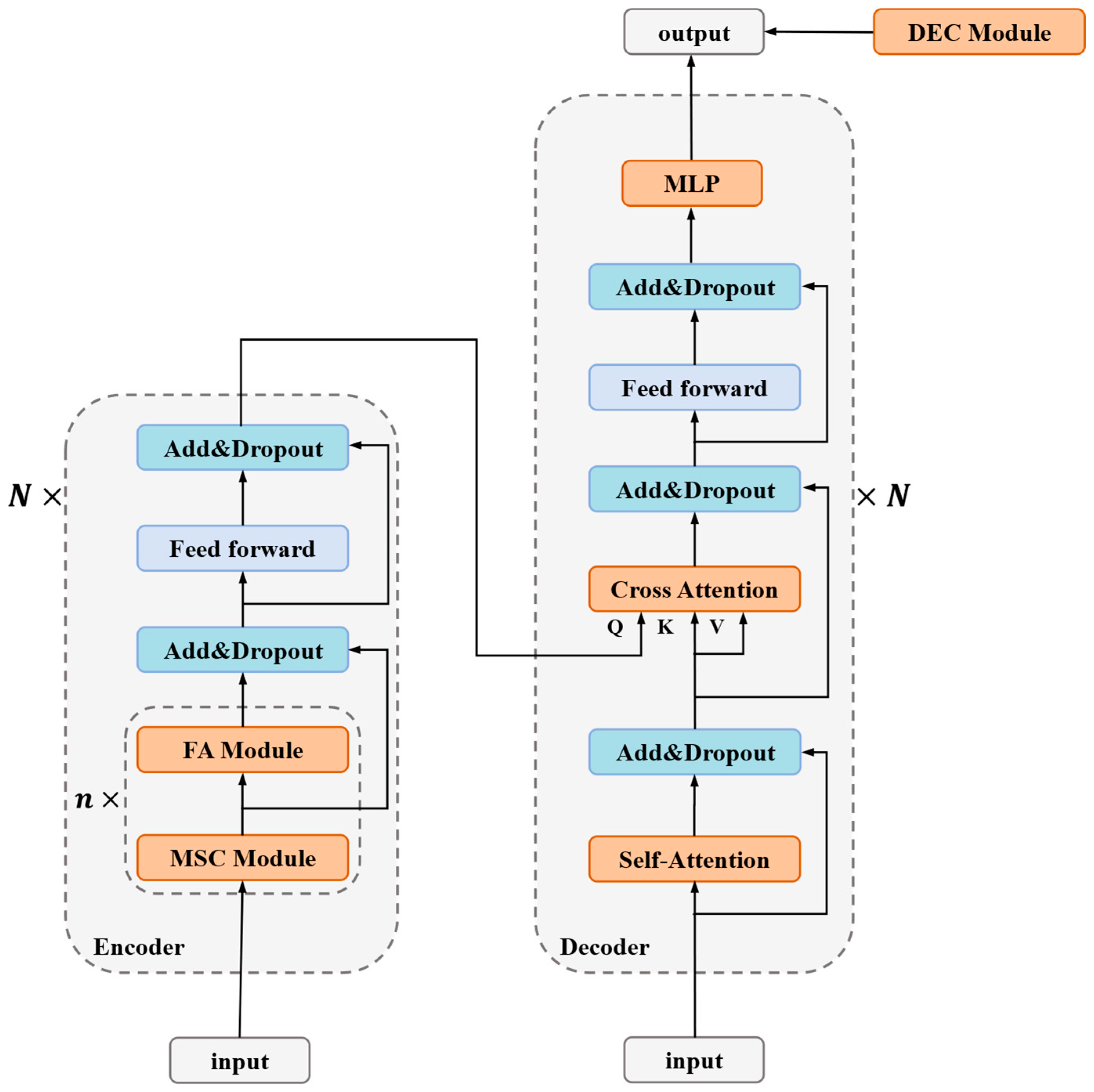Figure 1 is the overall architecture diagram of the model.

(1) The MF-Transformer model is constructed based on the MSC module and FA module, combined with transformer architecture, modeling the carbon market price time series and predicting the future trend. This model adopts a Transformer-based encoder-decoder architecture. The encoder processes and encodes the input time series, while the decoder generates predictions through iterative decoding.

(2) The encoder of the MF-Transformer model consists of MSC and FA modules, which decouple and model the multifractal characteristics of carbon market prices. The MSC module employs multi-layer dilated convolutions to decompose the time series into multi-scale components. The FA module calculates similarity weights between feature sequences at different scales to uncover the underlying multifractal structure of carbon market price series, thereby enhancing the model’s perception and understanding capabilities of complex dependency structures.

(3) The decoder of the MF-Transformer model adopts the standard Transformer decoder architecture, comprising self-attention, cross-attention, and feed-forward neural networks. It captures long-range dependencies in carbon market prices and dynamically integrates all extracted features for prediction.

(4) The DEC module is constructed based on the VAE model and an uncertainty-guided dynamic weighting mechanism to capture the latent distribution of error sequences and adaptively fuse the residual correction term with the underlying predicted values.

The MF-Transformer model is constructed by proposing multi-scale convolution, fractal attention, combined with a transformer architecture. And the DEC module is proposed for prediction error correction. The proposed method effectively models and accurately predicts multifractality, non-stationarity, multi-scale properties, and extreme volatility in carbon market price forecasting.

2.2. Implementation Principle of the MF-Transformer Core Module

2.2.1. Multi-Scale Convolution (MSC) Module

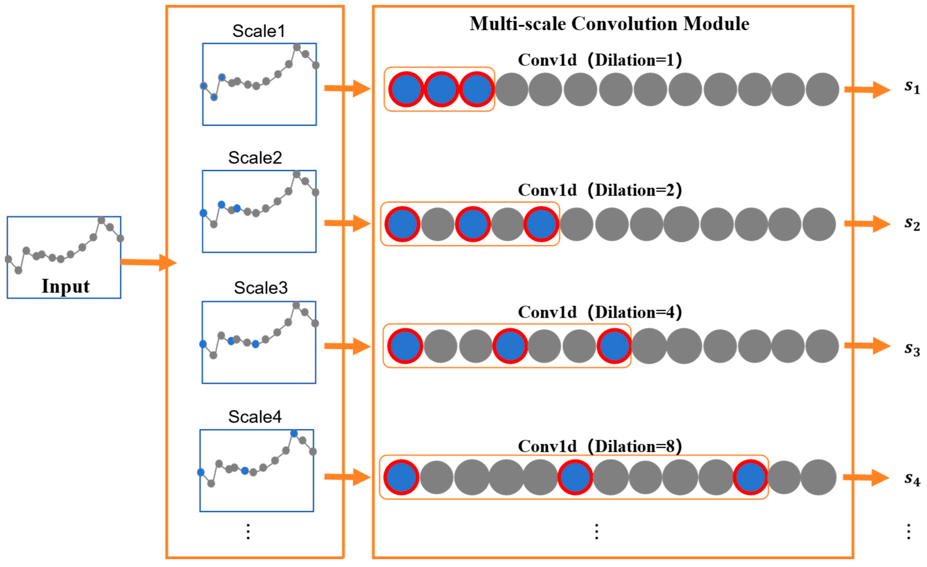
The carbon market price time series exhibits complex multifractality. However, most existing multi-scale carbon market price prediction methods rely on signal processing techniques and employ fixed decomposition approaches, lacking end-to-end learning capability, dynamic adaptability, and sophisticated feature modeling capacity. To address these limitations, a convolutional network with scale invariance is proposed in the MSC module. The MSC module adopts multiple dilated convolutional layers with varying dilation rates but shared convolutional kernel weights, endowing MSC with a learnable fractal perception capability. Compared with traditional convolution operations, dilated convolution employs interval sampling through hole filling, which expands the receptive field without increasing parameters or computational overhead, resulting in higher convolution efficiency. Figure 2 illustrates the schematic diagram of the multi-scale convolution principle.

The MSC module designs multiple layers of dilated convolutions where different dilated convolutional layers share the same convolutional kernel weights but employ exponentially increasing dilation rates. This creates a multi-layer convolutional structure that maintains identical feature extraction patterns while operating at different temporal scales, thereby projecting and reconstructing time series data within a multi-scale fractal space. Below, we detail the operation of a single dilated convolutional layer.

For a time series X = $\left\{{\mathrm{x}}_1,{\mathrm{x}}_2,\dots ,{\mathrm{x}}_{\mathrm{T}}\right\}$, Formula (1) represents the principle of the padding operation, Formula (2) represents the formula for performing dilated convolution with a dilation rate of d on the padded sequence, and Formula (3) represents the formula for applying the activation operation to the convolution output:

$${\tilde{\mathrm{x}}}_{\mathrm{i}}=\{\begin{array}{l}0,\mathrm{i}<1 \mathrm{o}\mathrm{r} \mathrm{i}>\mathrm{T}\\ {\mathrm{x}}_{\mathrm{i}},1<=\mathrm{i}<=\mathrm{T}\end{array},$$

(1)

$$\left\{{\mathrm{u}}_{\mathrm{t}}\right\}={\displaystyle \sum }_{\mathrm{n}=1}^{\mathrm{N}}{\mathsf{\omega }}_{\mathrm{n}}·{ \tilde{\mathrm{x}}}_{\mathrm{t}-\mathrm{d}·\left(\mathrm{n}-1\right)}\left(\mathrm{t}=1,2,\dots ,\mathrm{T}\right),$$

(2)

$$\left\{{\mathrm{z}}_{\mathrm{t}}\right\}=\mathrm{RELU}\left(\left\{{\mathrm{u}}_{\mathrm{t}}\right\}\right)\left(\mathrm{t}=1,2,\dots ,\mathrm{T}\right),$$

(3)

where ${ \tilde{\mathrm{x}}}_{\mathrm{i}}$ represents the result of one time step after the padding operation; $\left\{{\mathrm{u}}_{\mathrm{t}}\right\}\left(\mathrm{t}=1,2,\dots ,\mathrm{T}\right)$ is the output of the dilated convolution operation with dilation rate d; $\left\{{\mathsf{\omega }}_1,{\mathsf{\omega }}_2,\dots ,{\mathsf{\omega }}_{\mathrm{N}}\right\}$ denotes the original convolution kernel weights before dilation; ReLU is the activation layer that introduces nonlinearity, enabling the model to learn complex functional mappings; $\left\{{\mathrm{z}}_{\mathrm{t}}\right\}\left(\mathrm{t}=1,2,\dots ,\mathrm{T}\right)$ is the output after activation.

The dilation rates of different dilated convolutional layers vary. To progressively expand the receptive field, we adopt exponentially increasing dilation rates as shown in Formula (4). Different dilation rates correspond to different receptive fields, with the receptive field calculation formula given in Formula (5):

$$\mathrm{d}\in \left\{2^0,2^1,\dots ,2^{\mathrm{m}-1}\right\},$$

(4)

$$\mathrm{Receptive} \mathrm{Field}=\mathrm{d}·(\mathrm{N}-1)+1,$$

(5)

where 0, 1, …, m denotes the exponential order of dilation rate growth; d represents the dilation rate value, which belongs to an exponentially increasing set of dilation rates; N indicates the receptive field size of standard convolution.

2.2.2. Fractal Attention Module (FA)

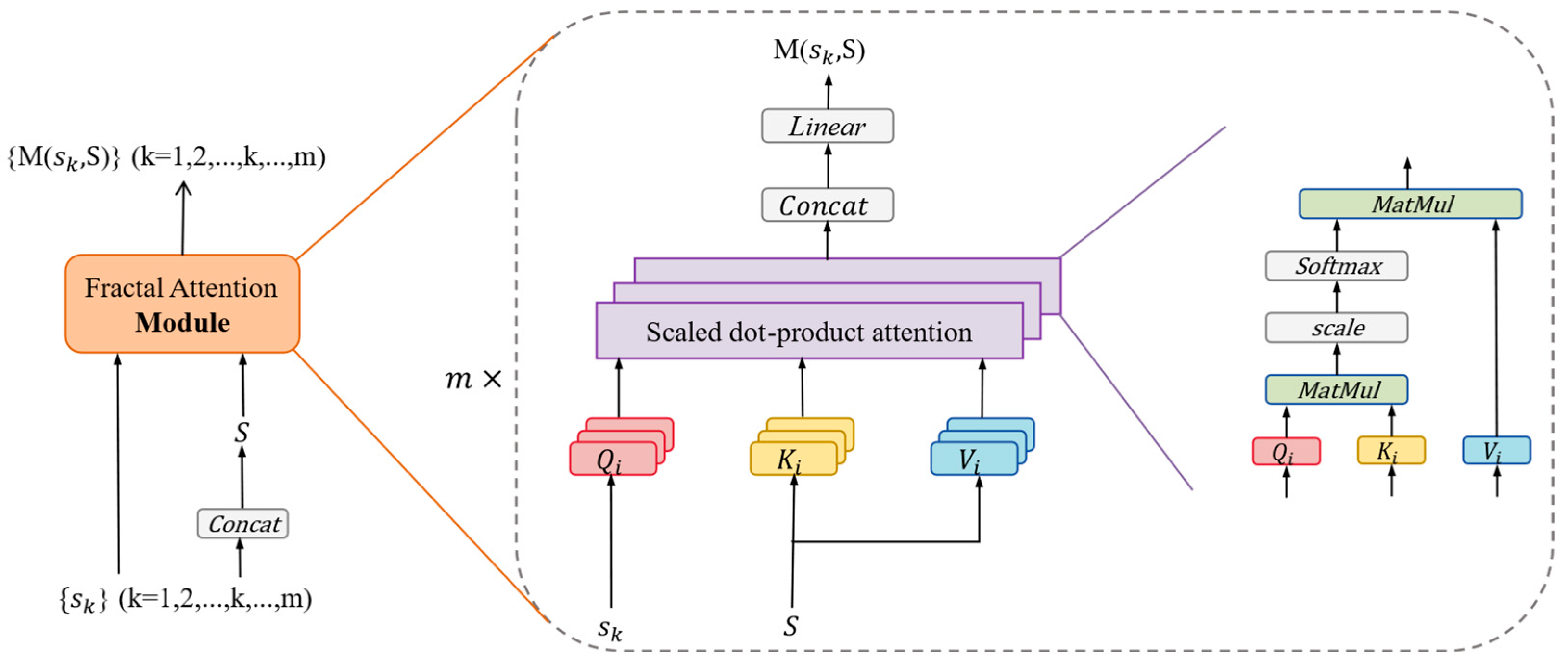
Carbon market price variations exhibit significant nonlinear dynamic characteristics and prominent non-stationarity, constituting a complex system with implicit multifractality. Existing carbon market price prediction models struggle to effectively capture the intricate temporal dynamics and suffer from issues such as gradient vanishing or explosion. To address this, we propose FA module, which employs multi-head attention to mine similarities across different scales and model multifractality in the data. Figure 3 illustrates the schematic diagram of fractal attention.

The output of one MSC module is connected to an FA module, where the FA module models latent dependencies in the data by computing similarities between different scales. The calculation of similarity between the k-scale and all scales is illustrated below as an example. Formula (6) is the calculation formula for concatenating all dilated convolution output vectors ${\mathrm{s}}_1$, ${\mathrm{s}}_2$, …, ${\mathrm{s}}_{\mathrm{k}}$, …, ${\mathrm{s}}_{\mathrm{m}}$ to obtain the vector S, containing the feature vectors from all scales. Formula (7) is the calculation formula for the query vector ${\mathrm{Q}}_{\mathrm{i}}$ corresponding to ${\mathrm{s}}_{\mathrm{k}}$ which is the convolution output of scale k, as well as the key vector ${\mathrm{K}}_{\mathrm{i}}$ and value vector ${\mathrm{V}}_{\mathrm{i}}$ corresponding to S, i $\in \left[1,\mathrm{h}\right]$ represents the i-th attention head. Formula (8) is the calculation formula for the similarity score $\mathrm{Score}$(${\mathrm{Q}}_{\mathrm{i}}$,${\mathrm{K}}_{\mathrm{i}}$) between the ${\mathrm{Q}}_{\mathrm{i}}$ and the ${\mathrm{K}}_{\mathrm{i}}$, obtained by the dot product. Formula (9) computes the weighted sum over each position based on the $\mathrm{Score}$(${\mathrm{Q}}_{\mathrm{i}}$,${\mathrm{K}}_{\mathrm{i}}$) to obtain the output of the attention mechanism Attention(${\mathrm{Q}}_{\mathrm{i}}$,${\mathrm{K}}_{\mathrm{i}}$,${\mathrm{V}}_{\mathrm{i}}$). Formula (10) is the calculation formula for the multi-head attention output M(${\mathrm{s}}_{\mathrm{k}}$,S) at ${\mathrm{s}}_{\mathrm{k}}$ on S. Different attention heads focus on different correlation relationships, facilitating comprehensive latent dependency mining.

$$\mathrm{S}=\mathrm{Concat}({\mathrm{s}}_1, {\mathrm{s}}_2, \dots , {\mathrm{s}}_{\mathrm{k}}, \dots , {\mathrm{s}}_{\mathrm{m}},\dim =-1),$$

(6)

$${\mathrm{Q}}_{\mathrm{i}}={\mathrm{s}}_{\mathrm{k}}{\propto }_{\mathrm{i}},{ \mathrm{K}}_{\mathrm{i}}={\mathrm{S}\mathsf{\beta }}_{\mathrm{i}},{ \mathrm{V}}_{\mathrm{i}}={\mathrm{S}\mathsf{\gamma }}_{\mathrm{i}},$$

(7)

$$\mathrm{Score}({\mathrm{Q}}_{\mathrm{i}},{\mathrm{K}}_{\mathrm{i}})=\mathrm{Q}{{\mathrm{K}}_{\mathrm{i}}}^{\mathrm{T}},$$

(8)

$$\mathrm{Attention}({\mathrm{Q}}_{\mathrm{i}},{\mathrm{K}}_{\mathrm{i}},{\mathrm{V}}_{\mathrm{i}})=\mathrm{Softmax}(({\displaystyle \frac{\mathrm{Score}\left(\mathrm{Q},\mathrm{k}\right)}{\sqrt{{\mathrm{D}}_{\mathrm{key}}}}})){\mathrm{V}}_{\mathrm{i}},$$

(9)

$$\mathrm{M}({\mathrm{s}}_{\mathrm{k}},\mathrm{S})=\mathrm{Concat}(\mathrm{Attention}({\mathrm{Q}}_1,{\mathrm{K}}_1,{\mathrm{V}}_1), \dots , \mathrm{Attention}({\mathrm{Q}}_{\mathrm{h}},{\mathrm{K}}_{\mathrm{h}},{\mathrm{V}}_{\mathrm{h}}\left)\right),$$

(10)

Concat(*,dim = −1) denotes concatenation along the last dimension; ${\propto }_{\mathrm{i}},{ \mathsf{\beta }}_{\mathrm{i}}$, ${\mathsf{\gamma }}_{\mathrm{i}}$ are trainable weight matrices ${\mathrm{D}}_{\mathrm{key}}$ is the dimension of keys.

By introducing the multi-head attention mechanism, we enable autonomous learning of similarity relationships across multiple scales to model the multifractal market dynamics, thereby enhancing the model’s understanding of complex systems and improving prediction accuracy.

2.2.3. MF-Transformer

The MF-Transformer model employs the transformer’s encoder-decoder architecture for integrated carbon market price prediction.

The encoder consists of MSC, FA, and other modules to model the multifractality of carbon market price series. Each MSC-FA combination extracts multi-scale similarity features. Multiple such parallel combinations can be configured, with different MSC modules in each combination using distinct convolutional kernel parameters to model time series through varied feature extraction patterns. These different combinations capture diverse feature types, achieving complementary feature learning and enabling comprehensive feature extraction from the time series.

The decoder consists of conventional self-attention, cross-attention, and feed-forward neural networks, featuring high modularity and scalability. The self-attention mechanism captures long-range dependencies within the sequence to enhance model generalization, as shown in Equation (11). The cross-attention dynamically integrates the fractal features extracted by the decoder with the long-range dependencies captured by self-attention, as shown in Equation (12):

$${\mathrm{R}}_2=\mathrm{SelfAttention}\left(\mathrm{X}\right)=\mathrm{M}(\mathrm{X},\mathrm{X}),$$

(11)

$$\mathrm{F}=\mathrm{CrossAttention}({\mathrm{R}}_1,{\mathrm{R}}_2)=\mathrm{M}({\mathrm{R}}_1,{\mathrm{R}}_2),$$

(12)

where $\mathrm{X}$ is the input time series ${\mathrm{R}}_1$ represents the encoder’s computation results; ${\mathrm{R}}_2$ denotes the self-attention computation results in the decoder; M($\mathrm{X}$,$\mathrm{X}$) indicates multi-head attention computation on $\mathrm{X}$; M(${\mathrm{R}}_1$,${\mathrm{R}}_2$) represents ${\mathrm{R}}_1$ computes multi-head attention on ${\mathrm{R}}_2$; F is the output after cross-attention fusion.

Residual connections with dropout are applied to prevent overfitting, followed by ReLU activation, as expressed in the following formula:

$$\mathrm{E}=\mathrm{ReLU}(\mathrm{F}+\mathrm{Dropout}(\mathrm{F}+\mathrm{M}({\mathrm{R}}_1,{\mathrm{R}}_2\left)\right)),$$

(13)

where Dropout denotes the dropout operation; M(${\mathrm{R}}_1$,${\mathrm{R}}_2$) represents ${\mathrm{R}}_1$ computes multi-head attention on ${\mathrm{R}}_2$; ReLU indicates the ReLU activation function operation; $\mathrm{E}$ is the final output result.

The feed-forward neural network utilizes the extracted features for prediction. The fused data is flattened and fed into a multi-layer perceptron (MLP), where linear transformation layers map the data to different dimensional spaces. Nonlinear feature transformation is achieved through ReLU activation, ultimately yielding the prediction result. The formula is as follows:

$$\hat{\mathrm{y}}=\mathrm{ReLU}({\mathrm{W}}_2\left(\mathrm{ReLU}\right({\mathrm{W}}_1\mathrm{Flatten}\left(\mathrm{E}\right)+{\mathrm{b}}_1\left)\right)+{\mathrm{b}}_2),$$

(14)

where $\hat{\mathrm{y}}$ is the final prediction; ${\mathrm{W}}_1$ represents the weight matrix from input to hidden layer; ${\mathrm{W}}_2$ denotes the weight matrix from hidden to output layer; ${\mathrm{b}}_1$ is the bias term for the hidden layer; ${\mathrm{b}}_2$ is the bias term for the output layer; ReLU indicates the ReLU nonlinear activation function; Flatten represents the flattening operation.

2.3. Dynamic Error Correction (DEC) Module

To enhance the carbon market price prediction model’s capability to analyze complex market fluctuations, the DEC module employs a Variational Autoencoder (VAE) to learn the latent distribution of errors and dynamically weights them for error correction in carbon market price sequences.

The VAE captures both temporal and distributional characteristics of error sequences, enabling it to learn the fractal commonality and extract the “de-randomized” core error properties. The VAE models the latent distribution of data through hidden variables and has strong regularization properties that prevent overfitting. Formula (15) is the calculation formula for activating the error sequence $\mathsf{ϵ}$. Formula (16) is the calculation formula for sampling the hidden variable z from a Gaussian distribution using the reparameterization technique. Formula (17) is the calculation formula for activating z. Formula (18) is the calculation formula for prediction output $\widehat{\mathsf{ϵ}}$.

$${\mathrm{h}}_1=\mathrm{Relu}({\mathrm{W}}_3\mathsf{ϵ}+{\mathrm{b}}_3),$$

(15)

$$\mathrm{z}=\mathsf{\mu }+\mathsf{\sigma }·{\mathsf{ϵ}}_{\mathrm{noise}},$$

(16)

$${\mathrm{h}}_2=\mathrm{Relu}({\mathrm{W}}_4\mathrm{z}+{\mathrm{b}}_4),$$

(17)

$$\widehat{\mathsf{ϵ}}={\mathrm{W}}_{\mathrm{out}}{\mathrm{h}}_2+{\mathrm{b}}_{\mathrm{out}},$$

(18)

where ${\mathrm{W}}_3$, ${\mathrm{W}}_4$ are hidden layer weights; ${\mathrm{b}}_3$, ${\mathrm{b}}_4$ are hidden layer bias terms; ReLU denotes the ReLU activation function; $\mathsf{\mu }$ represents the mean of ${\mathrm{h}}_1$; σ is the standard deviation of ${\mathrm{h}}_1; {\mathsf{ϵ}}_{\mathrm{noise}}$ is noise sampled from standard normal distribution; ${\mathrm{W}}_{\mathrm{out}}$ and ${\mathrm{b}}_{\mathrm{out}}$ are output layer weight and bias.

Traditional error compensation models using fixed error weights often lead to overfitting risks and struggle to adapt to the non-stationary volatility characteristics of carbon market price series. We utilize standard deviation to quantify uncertainty in error sequences and dynamically adjust the main model’s predictions. Formula (19) is the calculation formula for the uncertainty-driven dynamic weighting coefficient $\mathsf{\alpha }$. Formula (20) is the formula for dynamically weighting the error compensation $\widehat{\mathsf{ϵ}}$ back into the initial prediction value $\hat{\mathrm{y}}$.

$$\mathsf{\alpha }=1/(1+\mathsf{\sigma }),$$

(19)

$$\widehat{{\mathrm{y}}_{\mathrm{c}}}= \hat{\mathrm{y}}+\mathsf{\alpha }·\widehat{\mathsf{ϵ}},$$

(20)

where $\mathsf{\sigma }$ is the standard deviation of ${\mathrm{h}}_1$; $\widehat{\mathsf{ϵ}}$ denotes the error generated by the VAE model; $\widehat{{\mathrm{y}}_{\mathrm{c}}}$ is the final output after error compensation.

Compared with traditional fixed-weight methods, this strategy dynamically adjusts fusion weights based on σ’s uncertainty, significantly reducing interference from abnormal fluctuations while enhancing long-term trend fitting capability.

3. Results

This section describes the experimental data, multifractal analysis of carbon market prices, performance metrics, parameter settings, training and prediction process.

3.1. Description of Experimental Data

We construct forecasting tasks based on high-frequency data from China’s Shanghai and Guangdong carbon markets. The Shanghai carbon price dataset covers the Shanghai carbon market price series from 19 December 2013 to 30 August 2024, with a total of 1800 carbon price time-point data; the Guangdong carbon price dataset covers the Guangdong carbon market price series from 12 October 2016 to 30 August 2024, with a total of 1845 carbon price time-point data. The Shanghai carbon market price dataset is visualised in Figure 4 below, and the Shanghai carbon market price dataset is visualised in Figure 5 below.

The statistical characteristics of the Shanghai and Guangdong carbon market price datasets are shown in

Table 1. Table of Statistical Characteristics of Shanghai Carbon Market Price Dataset and Guangdong Carbon Market Price Dataset.

Statistical Characteristics	Shanghai Carbon Price Dataset	Guangdong Carbon Price Dataset
Mean	43.67	40.35
Median	40.16	28.99
Standard deviation	17.10	24.87
Range	73.47	85.46
Max	77.67	95.26
Min	4.20	9.80
Skewness	0.03	0.51
Kurtosis	−0.30	−1.27

. According to the data in the table:

For the Shanghai carbon price dataset, the mean is 43.67 and the median is 40.16. The standard deviation is 17.10, indicating a moderate level of price volatility and suggesting a certain degree of regularity in price fluctuations. The range is 73.47, determined by a maximum value of 77.67 and a minimum value of 4.20, indicating a notable historical fluctuation interval. The skewness is 0.03, showing that the price distribution is nearly symmetric with no significant skew. The kurtosis is −0.30, a negative value suggesting that extremely high and low prices occur less frequently.

For the Guangdong carbon price dataset, the mean is 40.35 and the median is 28.99, which is significantly lower than the mean, indicating a right-skewed distribution. The standard deviation is 24.87, a relatively large value, reflecting higher price volatility and a less stable market. The range is 85.46, composed of a maximum value of 95.26 and a minimum value of 9.80, indicating a wide historical variation in prices. The skewness is 0.51, a positive value indicating right skewness in the price distribution. The kurtosis is −1.27, also negative, indicating a low frequency of extreme values.

3.2. Multifractal Analysis of Carbon Market Price Series

The carbon market price variation exhibits notable nonlinear dynamical characteristics and pronounced non-stationarity, constituting a complex system with multifractal properties. We employ the Multifractal Detrended Fluctuation Analysis (MFDFA) method from the perspective of mathematical statistical analysis to verify the multifractal characteristics of the carbon market price datasets for Shanghai and Guangdong, thereby demonstrating the practical value of the proposed model.

The following introduction to the MFDFA method is based on the work of Kantelhardt et al. [29]. The specific steps of MFDFA are as follows:

(1) Calculate the dispersion sequence $\left\{{\mathrm{y}}_{\mathrm{i}}\right\}$ of the time series $\left\{{\mathrm{x}}_{\mathrm{i}}\right\}$(i = 1, 2, …, N),

$$\left\{{\mathrm{y}}_{\mathrm{i}}\right\}={{\displaystyle \sum }}_{\mathrm{k}=1}^{\mathrm{i}}\left({\mathrm{x}}_{\mathrm{k}}- \overline{\mathrm{x}}\right) (\mathrm{i}=1,2,\dots ,\mathrm{N}),$$

(21)

Here $\overline{\mathrm{x}}$ represents the mean value,

(2) Divide the sequence $\left\{{\mathrm{y}}_{\mathrm{i}}\right\}$ into ${\mathrm{N}}_{\mathrm{s}}=\mathrm{int}\left(\mathrm{N}/\mathrm{s}\right)$ intervals. Each interval contains s data points. When N is not divisible by s, ${\mathrm{y}}_{\mathrm{i}}$ will be a remainder. To avoid losing data, the division process is repeated from the end of the sequence, and ultimately, two equal-length subintervals are obtained, encompassing all the data points in the sequence.

(3) Calculate the mean squared error ${\mathrm{F}}^2\left(\mathrm{s},\mathrm{v}\right)$. Taking the interval v (v = 1, 2, …, 2${\mathrm{N}}_{\mathrm{s}}$) as an example, perform k-order polynomial fitting:

$${\mathrm{y}}_{\mathrm{v}}\left(\mathrm{i}\right)={\mathrm{a}}_1{\mathrm{i}}^{\mathrm{k}}+{\mathrm{a}}_2{\mathrm{i}}^{\mathrm{k}-1}+\dots +{\mathrm{a}}_{\mathrm{k}+1} (\mathrm{i}=1,2,\dots \mathrm{N}),$$

(22)

For the interval (v = 1, 2,…, 2$N_s$):

$${\mathrm{F}}^2(\mathrm{s},\mathrm{v})={\displaystyle \frac{1}{\mathrm{s}}}{{\displaystyle \sum }}_{\mathrm{i}=1}^{\mathrm{s}}\left\{\mathrm{y}\left[\left(\mathrm{v}-1\right)\mathrm{s}+\mathrm{i}\right]-{\mathrm{y}}_{\mathrm{v}}\left(\mathrm{i}\right)\right\},$$

(23)

For the interval (v = $N_s$ + 1,$N_s$ + 2, …, 2$N_s$):

$${\mathrm{F}}^2(\mathrm{s},\mathrm{v})={\displaystyle \frac{1}{\mathrm{s}}}{{\displaystyle \sum }}_{\mathrm{i}=1}^{\mathrm{s}}\left\{\mathrm{y}\left[\mathrm{N}-\left(\mathrm{v}-{\mathrm{N}}_{\mathrm{s}}\right)\mathrm{s}+\mathrm{i}\right]-{\mathrm{y}}_{\mathrm{v}}\left(\mathrm{i}\right)\right\},$$

(24)

(4) Calculate the q-order fluctuation function F(q,s):

$$\mathrm{F}(\mathrm{q},\mathrm{s})={\left\{{\displaystyle \frac{1}{2{\mathrm{N}}_{\mathrm{s}}}}{{\displaystyle \sum }}_{\mathrm{v}=1}^{2{\mathrm{N}}_{\mathrm{s}}}{[{\mathrm{F}}^2\left(\mathrm{s},\mathrm{v}\right)]}^{\mathrm{q}/2}\right\}}^{1/\mathrm{q}},$$

(25)

In the formula, q is a non-zero real number, and F(q,s) exhibits a power-law relationship with s.

(5) Calculate the individual generalized Hurst exponent h(q). Take q as a certain value and s as different values, repeat steps (26)–(28), and take the logarithm of F(q,s). Fit the slope of the curve to obtain the generalized h(q) value:

$$\ln \mathrm{F}\left(\mathrm{q},\mathrm{s}\right)=\ln \mathrm{k}+\mathrm{h}\left(\mathrm{q}\right)·\ln \mathrm{s},$$

(26)

(6) Calculate the generalized Hurst exponent and singularity exponent. Repeat steps (25)–(29) with different values of q to obtain them. Calculate the area and its width according to the following formula:

$$\mathsf{\alpha }\left(\mathrm{q}\right)=\mathrm{h}\left(\mathrm{q}\right)+\mathrm{q}{\displaystyle \frac{\mathrm{dh}\left(\mathrm{q}\right)}{\mathrm{dq}}},$$

(27)

$$\mathrm{f}\left(\mathsf{\alpha }\right)=\mathrm{q}[\mathsf{\alpha }-\mathrm{h}\left(\mathrm{q}\right)]+1,$$

(28)

$$\Delta \mathsf{\alpha }={\mathsf{\alpha }}_{\max }-{\mathsf{\alpha }}_{\min },$$

(29)

In the formula, $\mathsf{\alpha }$ represents the singularity exponent, indicating the growth probability of each sub-interval, and its value is inversely proportional to the singularity; $\mathrm{f}\left(\mathsf{\alpha }\right)$ denotes the multifractal spectrum; $\Delta \mathsf{\alpha }$ represents the difference between the maximum and minimum probabilities, and a larger value indicates a more uneven sequence distribution and a stronger fractal intensity.

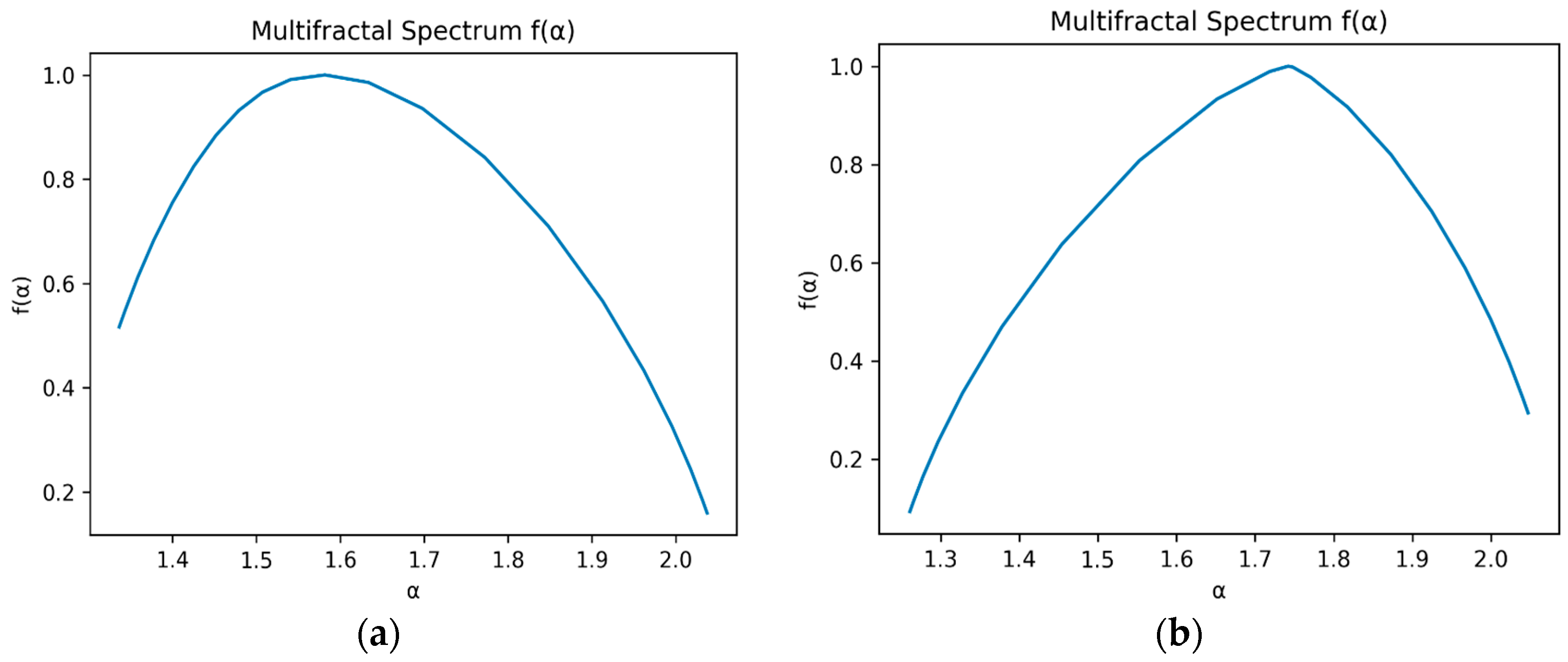
The multifractal spectrum of the Shanghai and Guangdong carbon market price datasets is shown in Figure 6. It can be concluded that the multifractal spectrum of the Shanghai carbon market price dataset is left-skewed, indicating that short-term fluctuations dominate. On the other hand, the multifractal spectrum of the Guangdong carbon market price dataset is right-skewed, indicating that long-term fluctuations dominate. The calculated value for the multifractal spectrum of the Shanghai carbon market price dataset is $\Delta \mathsf{\alpha }$ = 0.701 $>0$, while that of the Guangdong carbon market price dataset is $\Delta \mathsf{\alpha }$ = 0.786 $>0$, further confirming the multifractal nature of both datasets.

3.3. Performance Metrics

In this study, mean square residuals (MSE), mean absolute residuals (MAE), and root mean square residuals (RMSE) are selected as the evaluation indices to quantitatively evaluate the model’s prediction accuracy and robustness.

MAE is the average of absolute residuals. It is the average value of the absolute difference between the predicted value and the true value, which can intuitively reflect the average level of the prediction residuals. Its calculation formula is:

$$\mathrm{MAE}={\displaystyle \frac{1}{\mathrm{n}}}{{\displaystyle \sum }}_{\mathrm{i}=1}^{\mathrm{n}}|{\mathrm{y}}_{\mathrm{i}}-{ \hat{\mathrm{y}}}_{\mathrm{i}}{|}^2,$$

(30)

MSE is the expected value of the square of the difference between the estimated parameter and the true value. It can reflect the overall degree of variation in the predicted residuals. Its calculation formula is:

$$\mathrm{MSE}={\displaystyle \frac{1}{\mathrm{n}}}{{\displaystyle \sum }}_{\mathrm{i}=1}^{\mathrm{n}}{({\mathrm{y}}_{\mathrm{i}}-{ \hat{\mathrm{y}}}_{\mathrm{i}})}^2,$$

(31)

RMSE is the square root of the mean square residuals, and its unit is the same as the original data, which can reflect the size of the predicted residuals more intuitively. Its calculation formula is:

$$\mathrm{RMSE}=\sqrt{{\displaystyle \frac{1}{\mathrm{n}}}{{\displaystyle \sum }}_{\mathrm{i}=1}^{\mathrm{n}}{({\mathrm{y}}_{\mathrm{i}}-{ \hat{\mathrm{y}}}_{\mathrm{i}})}^2},$$

(32)

${\mathrm{R}}^2$ is used as an important indicator for assessing the performance of a regression model, which measures the model’s ability to explain the variance of the target variable. The range of values is usually between (−∞, 1).

$${\mathrm{R}}^2=1-{\displaystyle \frac{{{\displaystyle \sum }}_{\mathrm{i}=1}^{\mathrm{n}}{\left({\mathrm{y}}_{\mathrm{i}}-{ \hat{\mathrm{y}}}_{\mathrm{i}}\right)}^2}{{{\displaystyle \sum }}_{\mathrm{i}=1}^{\mathrm{n}}{\left({\mathrm{y}}_{\mathrm{i}}- \overline{\mathrm{y}}\right)}^2}},$$

(33)

In the above formula, n is the number of samples that have been validated, is the true value, is the predicted value of the model, is the mean of the actual value; the closer the values of MSE, MAE and RMSE are to 0, the better the predictive performance of the model. The closer the value is to 1, the better the explanatory ability of the model.

3.4. Parameter Settings

In this study, the parameter settings of the model have an important impact on the prediction performance. To ensure the stability and generalisation ability of the model, we optimised the key parameters through experiments and cross-validation. The specific parameter settings are shown in

Table 2. Core model hyperparameter settings.

Parameter Category	Parameter Name	Set Value
Model Architecture	dilations	[1, 2, 4, 8]
	kernel_size	3
	num_heads	4
	Dropout	0.1
Training strategy	Optimiser	Adam
	Loss function	MSE
	Batch size	32
	Training rounds (epochs)	60
	Random seed (random state)	42
	Regularisation factor λ1	1 × 10−4
	Regularisation factor λ2	1 × 10−3

:

The MSC module in the encoder part of the model uses a kernel size of 3 for the original convolution to extract local and global context information. The num_heads in multi-head attention is set to 4 to enhance the model’s ability to perceive features. Also, dropout is set to 0.1 to prevent overfitting.

The standard self-attention and cross-attention mechanisms in the decoder part of the model, num_heads and dropout, are used with settings consistent with the attention mechanism in the decoder.

During training, the Adam optimiser is used with the learning rate set to 1 × 10⁻³, the batch size set to 32, and the initial number of training rounds set to 10. The evaluation metrics include MSE, RMSE, MAE, and R² to comprehensively measure the model’s performance under different error metrics.

To enhance model robustness, a multi-level regularisation strategy is introduced. The L1 regularisation coefficient λ₁ = 1 × 10⁻⁴ is used to induce sparsity, and the L2 regularisation coefficient λ₂ = 1 × 10⁻³ is used to constrain the smooth variation of the mask function and enhance model stability.

3.5. Training and Prediction Process

The MF-Transformer-DEC’s modules work synergistically to achieve high-performance carbon market price prediction. The prediction process is shown in Figure 7. The specific processing steps are as follows:

Step 1: Data Pre-processing: Perform Z-score normalization on the original carbon market price series. Obtain a dataset using the sliding window method, and employ a sliding window technique with a fixed window length of 90 to construct a time series task that predicts the carbon market price trend for the next 7 days using the past 90 days. By defining a window function W(t) = [${\mathrm{x}}_{\mathrm{t}-89},{\mathrm{x}}_{\mathrm{t}-88}$, …, ${\mathrm{x}}_{\mathrm{t}}$] that slides continuously along the time axis with a unit stride (Stride=1), a set of observation subsequence samples {W(t)${\}}_{\mathrm{t}=90}^{\mathrm{T}}$ with strict temporal continuity, a form is formed. The sliding window method not only enhances the availability of training data but also ensures the integrity of sequence information, allowing for flexible construction of multi-step prediction datasets. A training-to-testing split ratio of 0.8:0.2 is adopted for the generated subsequence samples, which ensures sufficient model training while maintaining the effectiveness and comparability of the evaluation. The number of training and testing samples for 1-step, 3-step, and 7-step predictions in the Shanghai and Guangdong carbon market price datasets, which were obtained through the sliding window method and dataset partitioning, is presented in

Table 3. Table of training set sample sizes and testing set sample sizes for 1-step, 3-step, and 7-step predictions of the Shanghai carbon market price dataset and the Guangdong carbon market price dataset.

Dataset	Steps	Number of Samples in the Training Set	Number of Samples in the Testing Set
Shanghai carbon price dataset	1-step	1484	371
	3-step	1482	371
	6-step	1479	370
Guangdong carbon price dataset	1-step	1528	382
	3-step	1526	382
	6-step	1523	381
	1-step	1484	371

.

Step 2: Model Training: Initialize model parameters such as Dropout, and input the training dataset into the model for training.

Step 3: Model Prediction: Input the test dataset into the MF-Transformer model. The model outputs carbon market price prediction data for h time steps {$\widehat{{\mathrm{y}}_1}$, $\widehat{{\mathrm{y}}_2}$, …, $\widehat{{\mathrm{y}}_{\mathrm{p}}}$}.

Step 4: Residual prediction: Predict the residual sequence {${\mathsf{ϵ}}_1,{\mathsf{ϵ}}_2,\dots ,{\mathsf{ϵ}}_{\mathrm{p}}$} by inputting it into the VAE model for prediction, serving as the predicted values {$\widehat{{\mathsf{ϵ}}_1},\widehat{{\mathsf{ϵ}}_2},\dots ,\widehat{{\mathsf{ϵ}}_{\mathrm{p}}}$} for the carbon market price prediction residuals for h time points.

Step 5: Obtain the final forecast value of the carbon market price. The residual forecast results {$\widehat{{\mathsf{ϵ}}_1},\widehat{{\mathsf{ϵ}}_2},\dots ,\widehat{{\mathsf{ϵ}}_{\mathrm{p}}}$} for h time points are used to further optimize the original forecast results {$\widehat{{\mathrm{y}}_1}$, $\widehat{{\mathrm{y}}_2}$, …, $\widehat{{\mathrm{y}}_{\mathrm{h}}}$}, with the corrected carbon market price serving as the final carbon market price forecast value for the h time points.

4. Experimental Results and Discussion

The fifth part first constructs a multi-step prediction comparison experiment for the MF-Transformer model, then conducts ablation experiments, and finally evaluates the MF-Transformer model after dynamic residual correction. The performance advantages of the proposed model are verified through experiments from multiple aspects.

4.1. Multi-Step Prediction Comparison Experiment

The MF-Transformer proposed in this paper is compared and evaluated with SVR, LSTM, CNN, and Transformer. Based on high-frequency data from the carbon markets in Shanghai and Guangdong, China, a multi-step prediction task is constructed, utilizing carbon market price data from the past 90 time steps to predict future prices at 1, 3, and 7 time steps, respectively. Experimental results show that the MF-Transformer model proposed in this study significantly outperforms traditional methods in multi-dimensional evaluations. Compared to the benchmark models, its prediction accuracy and robustness have been significantly improved, and its key indicators surpass existing methods. The core advantage of this model stems from technological innovation in addressing the complex characteristics of carbon market price series.

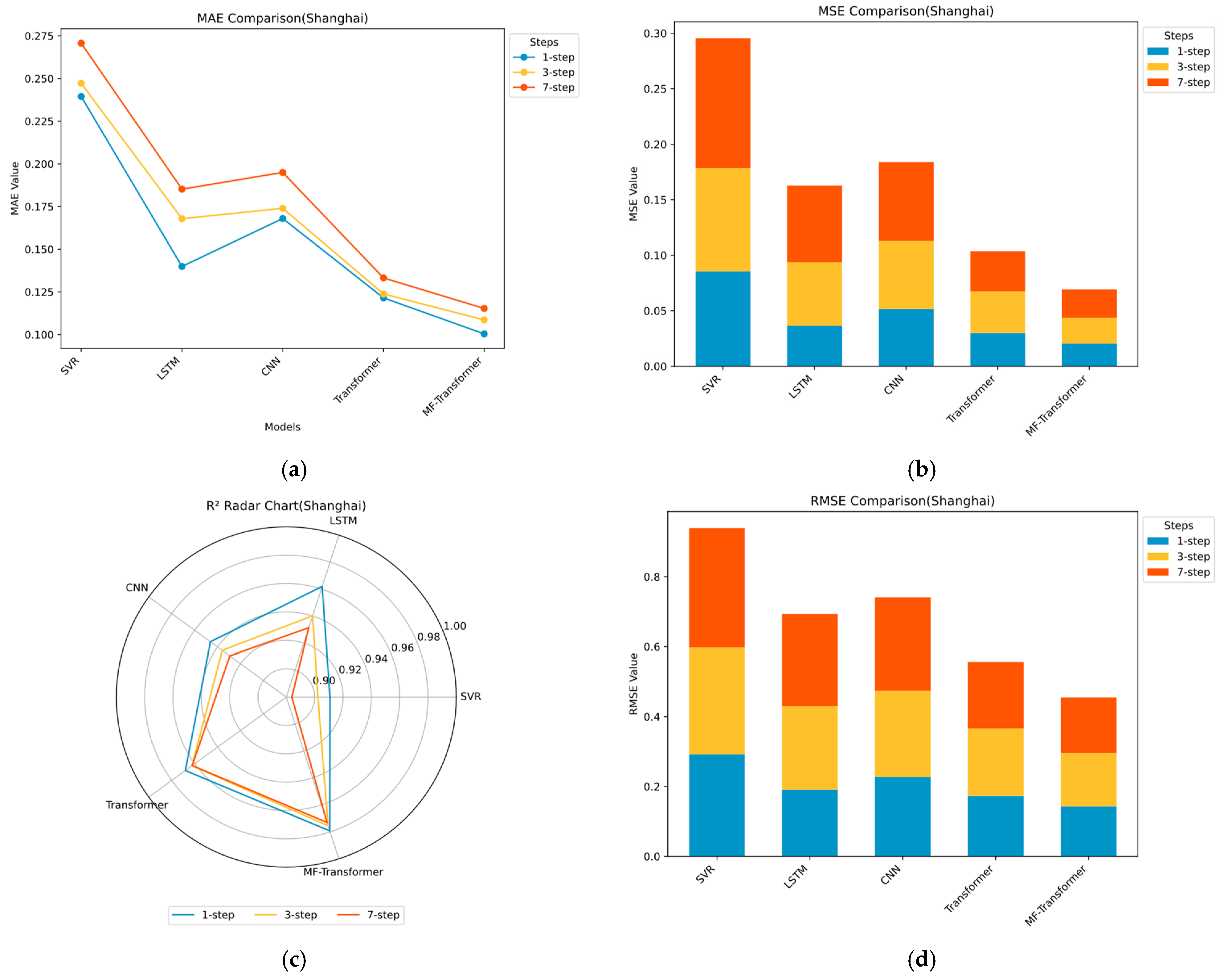
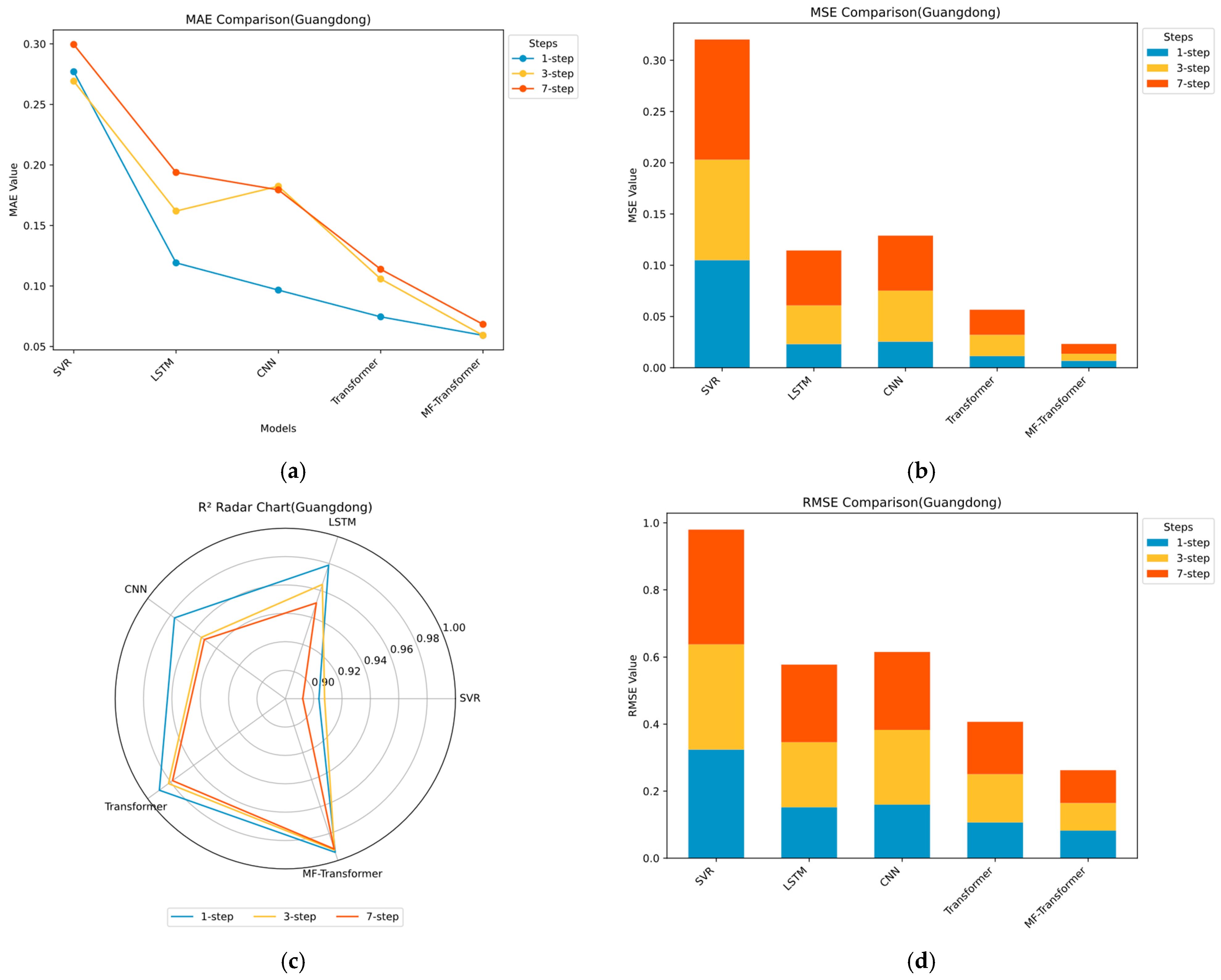
The experiment evaluates model performance using four quality metrics (detailed in Section 3.3 Performance Metrics). Mean Absolute Error (MAE) measures the average deviation between predicted and actual values; lower values indicate smaller overall prediction errors. Mean Squared Error (MSE) reflects the stability of the model under extreme conditions; smaller values suggest reduced variance in prediction errors. Root Mean Squared Error (RMSE), the square root of MSE, retains the same unit as the original data, making it easier to interpret the error magnitude; smaller RMSE values indicate better alignment between predicted and actual values. The coefficient of determination (R²) assesses the proportion of variance in the actual data that is explained by the model; values closer to 1 reflect stronger explanatory power.

The statistical results and visualizations of multi-step carbon price forecasting are presented in

Table 4. Evaluation Metrics Table for Multi-Step Forecasting on the Shanghai Carbon Market Price Dataset.

Steps	Experimental Group 1	MAE	MSE	RMSE	R2
1-step	SVR	0.2395	0.0855	0.2924	0.9108
	LSTM	0.1399	0.0365	0.1911	0.9619
	CNN	0.1680	0.0516	0.2271	0.9462
	Transformer	0.1215	0.0300	0.1732	0.9681
	MF-Transformer	0.1004	0.0204	0.1430	0.9792
3-step	SVR	0.2472	0.0932	0.3054	0.9023
	LSTM	0.1679	0.0572	0.2392	0.9401
	CNN	0.1740	0.0612	0.2473	0.9359
	Transformer	0.1238	0.0374	0.1933	0.9623
	MF-Transformer	0.1086	0.0233	0.1526	0.9755
7-step	SVR	0.2707	0.1168	0.3418	0.8839
	LSTM	0.1852	0.0691	0.2629	0.9313
	CNN	0.1950	0.0711	0.2667	0.9293
	Transformer	0.1332	0.0362	0.1903	0.9621
	MF-Transformer	0.1153	0.0255	0.1596	0.9730

and

Table 5. Evaluation Metrics Table for Multi-Step Forecasting on the Guangdong Carbon Market Price Dataset.

Steps	Experimental Group 2	MAE	MSE	RMSE	R2
1-step	SVR	0.2770	0.1050	0.3241	0.9037
	LSTM	0.1191	0.0231	0.1520	0.9788
	CNN	0.0966	0.0255	0.1598	0.9766
	Transformer	0.0745	0.0114	0.1066	0.9898
	MF-Transformer	0.0592	0.0068	0.0822	0.9939
3-step	SVR	0.2692	0.0980	0.3131	0.9077
	LSTM	0.1619	0.0377	0.1941	0.9645
	CNN	0.1824	0.0497	0.2229	0.9532
	Transformer	0.1058	0.0207	0.1440	0.9818
	MF-Transformer	0.0592	0.0068	0.0822	0.9922
7-step	SVR	0.2995	0.1173	0.3426	0.8923
	LSTM	0.1938	0.0536	0.2316	0.9508
	CNN	0.1794	0.0537	0.2318	0.9506
	Transformer	0.1138	0.0245	0.1564	0.9783
	MF-Transformer	0.0683	0.0096	0.0981	0.9914

and Figure 8 and Figure 9. The main findings are as follows: (1) The proposed MF-Transformer achieves the best overall performance across all metrics. On the Shanghai carbon price dataset, the average MAE, MSE, RMSE, and R² are 0.1081, 0.0231, 0.1517, and 0.9759, respectively. On the Guangdong dataset, the corresponding values are 0.0622, 0.0077, 0.0875, and 0.9925. These results demonstrate the model’s strong accuracy, generalization capability, and modeling effectiveness. (2) Deep learning models generally outperform traditional machine learning approaches. Traditional models such as SVR lack the ability to capture sequential dependencies, resulting in R² values ranging between 0.88 and 0.91 and MAE values exceeding 0.2. These figures indicate limited capability in capturing complex market dynamics and higher prediction errors. (3) The performance of LSTM and CNN models generally deteriorates as the forecast horizon increases. For instance, in the Guangdong dataset, LSTM’s MAE increases from 0.1191 at 1-step to 0.1938 at 7-step, and RMSE rises from 0.1520 to 0.2316, highlighting the limitations in long-term forecasting and weak generalization ability. (4) The Transformer model achieves higher prediction accuracy than other baseline models. In the 7-step prediction task on the Guangdong dataset, the Transformer model achieves an RMSE of 0.1564 and an R² of 0.9783, clearly outperforming LSTM and CNN, which supports the effectiveness of Transformer-based architectures. (5) MF-Transformer consistently delivers the best performance across all datasets. It maintains R² values above 0.97 and RMSE values below 0.15, outperforming other ensemble models. The consistent superiority and stability of MF-Transformer indicate its robustness and strong generalization ability, confirming its structural advantages in carbon price prediction tasks.

4.2. Ablation Experiment of MF-Transformer

Due to the excellent performance of the proposed method, which is generated by multiple modules, we conducted an ablation study. Since the prediction task of 7 time steps can verify the model’s performance on different prediction time scales and ensure the model’s generalization ability under multi-step prediction, the ablation experiment was based on the task of predicting carbon market prices for the next 7 time steps. The statistical results of the prediction evaluation metrics are presented in

Table 6. Evaluation Metrics Table for Ablation Experiments on the Shanghai Carbon Market Price Dataset.

Experimental Group 3	MAE	MSE	RMSE	R2
Single transformer	0.1332	0.0362	0.1903	0.9621
Remove MSC	0.1299	0.0345	0.1857	0.9653
Remove FA	0.1286	0.0303	0.1740	0.9680
MF-Transformer	0.1153	0.0255	0.1596	0.9730

and

Table 7. Evaluation metric table for ablation experiments on the Guangdong carbon market price dataset.

Experimental Group 4	MAE	MSE	RMSE	R2
Single transformer	0.1138	0.0245	0.1564	0.9783
Remove MSC	0.1006	0.0170	0.1305	0.9849
Remove FA	0.0909	0.0142	0.1191	0.9868
MF-Transformer	0.0683	0.0096	0.0981	0.9914

, from which it can be observed that: (1) the proposed model performs the best, indicating that the network architecture of the proposed model excels in carbon market price prediction. (2) The prediction performance of the other three methods declined to varying degrees, indicating that each module of the proposed method plays a positive role and further validates the rationality of the model design. When the MSC module is removed from the proposed model, its performance decreases. On the Shanghai dataset, the MAE increases from 0.1153 to 0.1299, and the R² drops from 0.9730 to 0.9653. On the Guangdong dataset, the MAE increases from 0.0683 to 0.1006, and the R² decreases to 0.9849. The simultaneous increase in prediction error and decrease in model fit suggest that the MSC module plays a crucial role in capturing temporal scale variations and enhancing the model’s fitting ability. Similarly, removing the FA module also leads to increased prediction errors. On the Shanghai dataset, the MAE rises to 0.1286 and the RMSE increases to 0.1740. On the Guangdong dataset, the MAE increases to 0.0909 and the RMSE rises to 0.1191. These results demonstrate that the FA module is essential for modeling the multifractal structure and reducing prediction errors. (3) The single transformer model yields the poorest prediction performance. On the Shanghai and Guangdong datasets, the MAE values are 0.1332 and 0.1138, respectively, and the R² values are only 0.9621 and 0.9783. While the proposed ensemble model achieves the highest prediction accuracy on the dataset, it demonstrates the importance of multi-scale complex temporal analysis and similarity modeling in predicting carbon market prices. In summary, the proposed method integrates the aforementioned three modules to ensure high-performance prediction results, further proving that each module plays its own positive role in improving prediction performance.

4.3. Evaluation Experiment of the DEC Mechanism and Model Stability Analysis

The statistical metrics from 15 repeated experiments of MF-Transformer-DEC on the Shanghai and Guangdong carbon market price datasets were used to evaluate the effectiveness of the DEC mechanism in correcting prediction errors of the MF-Transformer, while also verifying that the model’s performance is not due to chance. This eliminates the bias caused by single-run experimental randomness and demonstrates the model’s stable and statistically significant performance. Since the 7-step prediction task allows the evaluation of model performance across different forecast horizons, it serves as an effective test of the model’s generalization ability under multi-step prediction scenarios. Therefore, the evaluation of the dynamic error correction mechanism was conducted based on the task of forecasting carbon prices over the next 7 time steps.

Table 8. Table of mean and standard deviation of evaluation metrics for MF-Transformer-Dec running 15 times on Shanghai and Guangdong carbon market price datasets.

Experimental Group 5	MAE		MSE		RMSE		R2		MAE		MSE		RMSE		R2
	Mean	Std	Mean	Std	Mean	Std	Mean	Std	Mean	Std	Mean	Std	Mean	Std	Mean	Std
Shanghai Carbon Market Price Dataset	0.0983	0.0064	0.0219	0.0016	0.1478	0.0055	0.9777	0.0016	0.0983	0.0064	0.0219	0.0016	0.1478	0.0055	0.9777	0.0016
Guangdong Carbon Market Price Dataset	0.0485	0.0039	0.0059	0.0005	0.0773	0.0033	0.9942	0.0005	0.0485	0.0039	0.0059	0.0005	0.0773	0.0033	0.9942	0.0005

presents the mean and standard deviation of evaluation metrics obtained from 15 runs of MF-Transformer-DEC on the Shanghai and Guangdong datasets. The results show that: (1) Compared with MF-Transformer, MF-Transformer-DEC achieves over a 14% reduction in MAE and MSE on both datasets, indicating smaller prediction errors and higher forecasting accuracy. The R² of MF-Transformer-DEC is consistently higher, suggesting an improved ability to capture carbon price trends. These results confirm that the DEC mechanism significantly enhances prediction performance. (2) On the Shanghai dataset, the model achieved very low average MAE, MSE, and RMSE across 15 repeated experiments, with standard deviations all below 0.007, indicating both low prediction error and high consistency. The average R² reached 0.9777, meaning the model explains 97.77% of the price variance and demonstrates strong generalization ability. On the Guangdong dataset, the average MAE was only 0.0485, showing extremely low prediction error. The mean and standard deviation of MSE and RMSE were also low, reflecting high prediction precision. The R² reached 0.9942, with minimal standard deviation across 15 runs, indicating that the model accurately captures market fluctuations. (3) Across 15 independent repeated experiments on both datasets, MF-Transformer-DEC consistently achieved excellent average performance and small standard deviations for MAE, MSE, RMSE, and R². This confirms the model’s high fitting capability and robustness, effectively ruling out the possibility of accidental performance. It demonstrates that the model is stable and reliable.

4.4. Discussion

The proposed MF-Transformer-DEC, through the integration of fractal thinking and architectural innovation, demonstrates significant performance advantages in carbon market price prediction tasks. It breaks through the limitations of traditional methods and existing deep learning structures, providing a new solution and paradigm for complex time series modeling. In three experiments, the average evaluation metrics of MF-Transformer-DEC outperformed all other metrics, exhibiting remarkable advantages and strong modeling capabilities and generalization performance.

In the aspect of multi-scale modeling, MF-Transformer-DEC employs multiple layers of dilated convolutions to capture variation patterns at different temporal scales, enabling fully end-to-end learning. Existing multi-scale modeling approaches often rely on fixed signal processing techniques such as discrete wavelet transform (DWT), variational mode decomposition (VMD), and ensemble empirical mode decomposition (EEMD), which involve complex decomposition procedures and are difficult to unify within a trainable framework. The proposed model addresses these limitations by integrating multi-scale modeling directly within the deep learning architecture, jointly training it with the backbone network. This approach overcomes the separation of decomposition and prediction, non-learnable parameters, and strong dependence on prior assumptions seen in traditional methods, significantly enhancing the model’s dynamic adaptability and its ability to represent complex, non-stationary temporal features.

In the aspect of multifractal modeling, MF-Transformer-DEC introduces innovative methods and carefully designed modules to dynamically perceive and effectively model multifractal characteristics using deep learning. Traditional fractal modeling techniques primarily depend on mathematical statistical methods, including multifractal detrended fluctuation analysis (MFDFA), asymmetric MFDFA (A-MFDFA), multifractal detrended cross-correlation analysis (MF-DCCA), fractal dimension calculation, and Hurst exponent estimation. These approaches focus on analysis without predictive capabilities, often involving complex workflows, heavy reliance on data pre-processing, and modular separation that hinders embedding into deep networks. MF-Transformer-DEC overcomes these issues by enabling MSA and FA modules to work synergistically, converting traditional fractal feature extraction from a static, non-trainable, and prediction-decoupled external process into an end-to-end trainable embedded module. This resolves the limitations of non-integrability and non-optimizability in conventional methods. The MSC module is designed as a scale-invariant convolutional network that adaptively extracts fractal features relevant to prediction through learnable convolution kernels. The FA module explicitly models potential multifractal structures in carbon price sequences by computing similarity weights among multi-scale convolution features, enabling cross-scale relational modeling and enhancing the model’s understanding of complex fluctuation patterns. This approach effectively improves the model’s adaptability to nonlinear features in carbon market price sequences, increasing prediction accuracy and generalization performance, and demonstrates a novel paradigm integrating fractal modeling with deep learning.

In the aspect of modeling long-range dependencies, MF-Transformer-DEC adopts a standard Transformer decoder architecture, comprising self-attention, cross-attention, and feed-forward networks, which provides strong capabilities for capturing global dependencies. In contrast, recurrent structures like LSTM and GRU, although possessing memory mechanisms, depend on sequential state updates, limiting parallelization and suffering from information decay across multiple steps. Such architectures often encounter vanishing gradient and information loss issues when processing long sequences or distant dependencies. The global modeling and parallel processing advantages of the decoder’s self-attention enable MF-Transformer-DEC to more accurately capture the propagation of long-distance fluctuations in the carbon market.

In the aspect of residual correction, MF-Transformer-DEC utilizes an uncertainty-guided dynamic weighted fusion strategy to address a common shortcoming in existing research, where prediction residuals are often ignored or treated with static adjustments. Compared with other methods that employ fuzzy entropy combined with EEMD for secondary residual decomposition, support vector regression for residual modeling, or BiLSTM for independent error learning—which, although improving accuracy to some extent, mostly rely on static modeling that neglects temporal variability and uncertainty in errors—MF-Transformer-DEC measures uncertainty of the residual sequence using standard deviation to guide adaptive weighted fusion. This dynamic compensation of prediction errors significantly enhances robustness under abnormal fluctuations and sudden market changes. Moreover, the VAE module employed is simple, with low parameter count, fast forward propagation, and minimal training overhead. Traditional approaches based on fuzzy entropy, differential evolution, or EEMD for secondary residual correction often depend on manual tuning and external algorithms, leading to complexity, limited interpretability, and difficulty in joint optimization within the model.

The proposed MF-Transformer-DEC model consistently delivers excellent results across multiple datasets, demonstrating strong transferability and broad applicability in various carbon market environments. Compared to traditional and existing deep integration models, it significantly reduces errors, facilitating more accurate guidance for policy formulation, market decision-making, and carbon asset management. This provides a solid model foundation for high-quality, deployable carbon market price prediction tasks.

5. Conclusions

This study proposes a Transformer model based on multi-scale convolution and fractal attention, incorporating a variational autoencoder (VAE) to model error distribution. By adaptively integrating the residual correction term with the baseline prediction value, the model enhances its ability to analyze the complex fluctuation characteristics of the energy market. The proposed model flexibly models the multifractality of carbon market prices and performs fusion prediction while introducing an uncertainty-guided dynamic residual prediction mechanism, significantly improving the prediction accuracy of complex carbon market price sequences. Experimental results demonstrate that the proposed model outperforms benchmark models in key metrics such as MAE, RMSE, and R², validating the effectiveness of the synergistic interaction between multi-scale extraction, similarity mining, and residual correction.

The primary limitation of this study lies in the insufficient consideration of exogenous variables, such as geographical factors, that may impact carbon market prices. Future research could introduce a dynamic variable selection mechanism to enhance model adaptability. Additionally, exploring the integration of multi-source heterogeneous data (e.g., satellite remote sensing carbon monitoring data) with the existing model represents a promising direction for expanding the model’s application scenarios.