Nonfragile State Estimator Design for Memristor-Based Fractional-Order Neural Networks with Randomly Occurring Hybrid Time Delays and Stochastic Cyber-Attacks

Abstract

This paper addresses the design of nonfragile state estimators for memristor-based fractional-order neural networks that are subject to stochastic cyber-attacks and hybrid time delays. To mitigate the issue of limited bandwidth during signal transmission, quantitative processing is introduced to reduce network burden and prevent signal blocking. In real network environments, the outputs may be compromised by cyber-attacks, which can disrupt data transmission systems. To better reflect the actual conditions of fractional-order neural networks, a Bernoulli variable is utilized to describe the statistical properties. Additionally, novel conditions are presented to ensure the stochastic asymptotic stability of the augmented error system through a new fractional-order free-matrix-based integral inequality. Finally, the effectiveness of the proposed estimation methods is demonstrated through two numerical simulations.

1. Introduction

It is widely recognized that fractional-order calculus (FOC) can be considered an extension of traditional integer-order calculus. It is important to note that the previous outstanding results for FOC have primarily been involved in theoretical research [1,2]. Until 1960, FOC was gradually being applied to various fields, such as mechanics, science, and biology [3,4,5,6]. Owing to the properties of infinite memory and heredity, FOC can describe real phenomena more accurately than integer-order calculus [1,7]. In recent decades, the system models described by FOC have attracted considerable research attention, and a great many results of synchronization and stability analysis have become available [8,9]. In [10], the authors investigated the design of an adaptive sliding mode controller for fractional-order singular systems with parameter uncertainties, utilizing both state and output feedback. Furthermore, event-triggered synchronization control based on sampled data for fractional complex networks with time-varying delays has been investigated [11], and a more general class of network structures has been taken into consideration.

Over the past few decades, neural networks (NNs) have garnered significant attention due to their diverse applications in various real-world contexts, including target tracking, signal processing, pinning control, and other scientific domains [12,13,14]. For these applications, it is essential to first verify the stability of NNs. This verification is crucial, as most of these applications primarily depend on the dynamic behavior of equilibrium points [15]. Notably, fractional-order derivatives are well suited to describing various materials and dynamical processes due to their memory and hereditary properties. Consequently, fractional-order derivatives are frequently employed to characterize different types of systems across multiple fields. To enhance understanding of the dynamical behavior of neurons, fractional-order neural networks (FONNs), which integrate fractional calculus with NNs, have been proposed.

It is well known that the state information of neurons plays a crucial role in the extensive application of NNs. However, NNs are constructed using large-scale integrated circuits. Given the constraints of limited measurement resources, it is challenging to directly obtain the state information of all neurons [14]. Therefore, investigating the state estimation (SE) problem of NNs is essential for addressing various real-world applications. In neural network circuit systems, the limited switching speed of amplifiers and the restricted speed of signal transmission result in inevitable time delays within these systems. 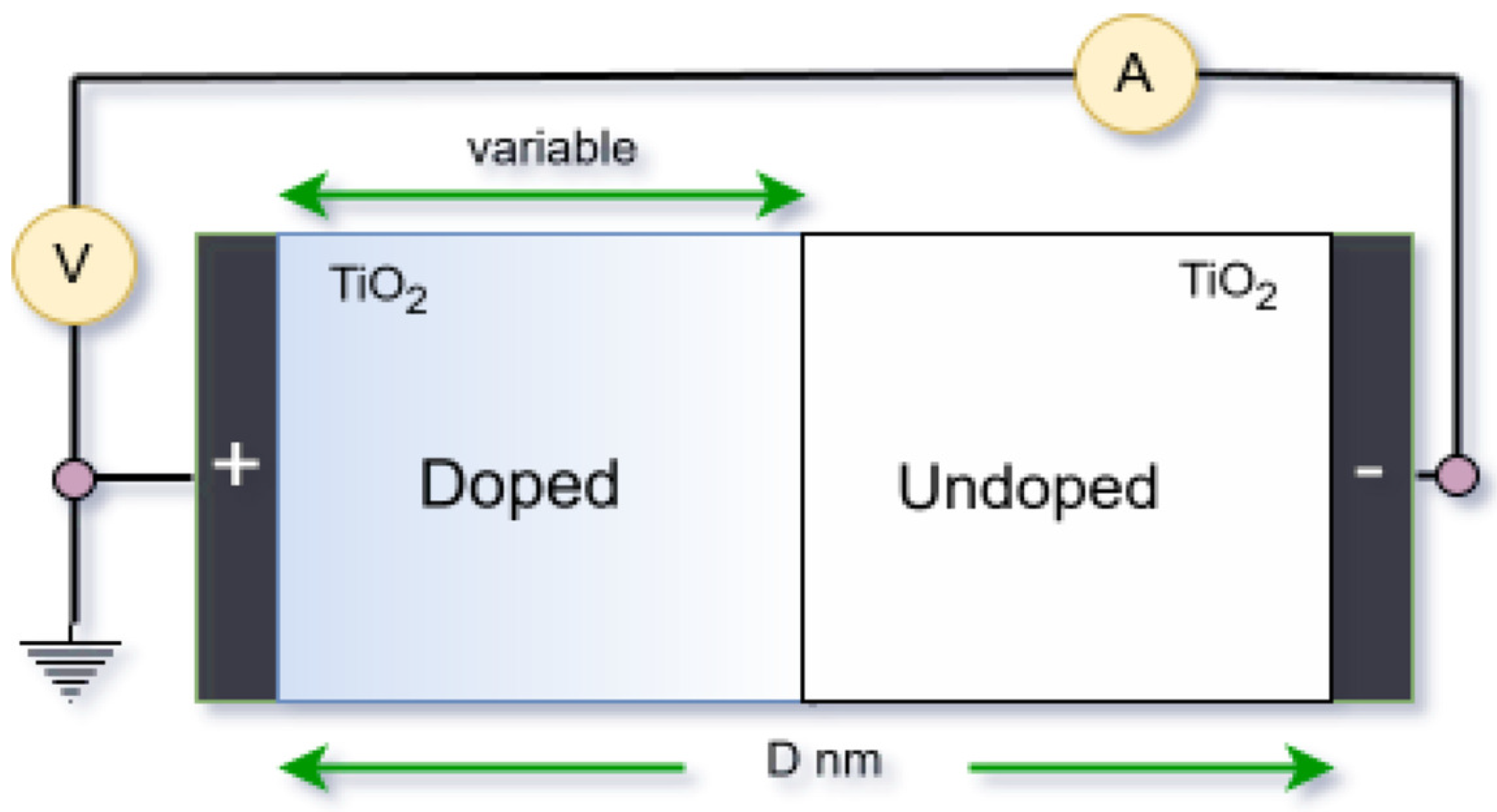The issue of SE for delayed NNs was first introduced in [16]. It is noteworthy that Chua first proposed the concept of the memristor in 1971 [17], and the initial memristor component was fabricated by HP Labs (shown in Figure 1). Distinct from traditional resistors, memristors reduce energy consumption, enhance operational speeds, and decrease memory space requirements. Therefore, memristors are frequently utilized in various complex systems, particularly within NNs. In [18], the issue of state estimation for memristor-based FONNs with time delays is addressed. By employing fractional-order Lyapunov methods, the authors present stability conditions that guarantee asymptotic stability. However, the results are delay-independent and exhibit a higher degree of conservatism. In [19], the author addresses the issue of event-based SE for FONNs with external disturbances. A delay- and order-dependent condition is provided to ensure the existence of a fractional-order state estimator. However, this criterion does not actually depend on delay or order, indicating that the condition is excessively conservative.

On the other hand, the performance of the estimator may be adversely affected by fluctuations resulting from variable environments, leading to fragility of the estimator. Therefore, it is essential to design a robust nonfragile state estimator for memristor-based FONNs. Currently, numerous design studies have concentrated on nonfragile estimators in integer-order systems. However, there is a relative scarcity of research addressing the issue of nonfragile SE in fractional systems. The nonfragile SE problem for memristor-based FONNs was examined with and without time delays in [18]. It is noteworthy that the results derived in [18] are delay-independent, indicating that the conditions may be overly conservative. Additionally, quantitative processing is often employed to conserve network resources in practice due to finite bandwidth limitations. In [21], the authors explore the synchronization issue of memristor-based FONNs with time delays through quantized control. Despite this, there are few studies focused on designing a fractional-order nonfragile estimator for memristor-based FONNs, which serves as the motivation for our research.

Time delays (TDs) are commonly observed in most physical systems, particularly in neural network circuit systems, due to the switching speed limitations of amplifiers [22]. The presence of TDs can result from oscillations and instabilities within NNs. Therefore, it is essential to take TDs into consideration when examining the dynamical behavior of NNs. In real-world environments, time delays may occur probabilistically, called randomly occurring time-varying delays (ROTVDs). This phenomenon has garnered significant attention from researchers. For example, the authors address the issue of resilient proportional-integral observers for Markov memristor-based neural networks (NNs) with sensor saturation and ROTVDs in [23]. The problem of partial-neuron-based state estimation for delayed NNs is addressed in [24]. To the best of our knowledge, there is limited research on fractional-order systems with ROTVDs, particularly in the context of NNs. Motivated by these considerations, our objective is to investigate the design of nonfragile state estimators for a class of memristor-based FONNs that are subject to ROTVDs and stochastic cyber-attacks. The key advantages of our investigation are outlined as follows:

(1)

The issue of nonfragile state estimator design for memristor-based FONNs is investigated subject to hybrid ROTVDs and stochastic cyber-attacks.

(2)

The traditional Lyapunov–Krasovskii functions (LKFs), which include derivative terms, are not suitable for fractional-order systems. In this paper, we construct several novel LKFs which contain fractional integral terms and time delay information. This approach implies that the results presented in this paper exhibit reduced conservatism.

(3)

Combining fractional-order Lyapunov approaches and a novel free-matrix-based integral inequality, several delay- and order-dependent criteria are derived to guarantee the asymptotic stability of the augmented system.

(4)

Due to the finite bandwidth and complex environment, a kind of fractional-order quantized nonfragile state estimator is developed for memristor-based FONNs. Finally, some numerical examples are shown to validate the usefulness of the proposed estimation algorithm.

2. Problem Formulation and Preliminaries

Definition 1

([25]). For the function $h\left(t\right)$, the fractional integral operator is defined as

$$\begin{array}{c}\hfill I^{\beta }h\left(t\right)={\displaystyle \frac{1}{\mathrm{\Gamma }\left(\beta \right)}}{\int }_a^t{(t-x)}^{\beta -1}h\left(x\right)dx,\beta \in {\mathbb{R}}^{+}\end{array}$$

where $t\ge a$ and the Gamma function $\mathrm{\Gamma }\left(z\right)={\int }_a^{\infty }{e}^{-t}{t}^{z-1}dt$.

Definition 2

([25]). Caputo’s derivative for function $h\left(t\right)$ is

$$\begin{array}{c}\hfill {}_a{}^{C}D_t^{\beta }h\left(t\right)={\displaystyle \frac{1}{\mathrm{\Gamma }(l-\beta )}}{\int }_a^t{(t-x)}^{l-\beta -1}{h}^{\left(l\right)}\left(x\right)dx,\end{array}$$

where $t\ge a$, and $\beta \in (l-1,l)$, $h\left(t\right)\in C^k([a,\infty ),\mathbb{R})$.

Let us consider the following memristor-based FONN models with time-varying delays:

$$\left\{\begin{array}{c}\begin{array}{cc}\hfill {}_{t_0}{}^{C}D_t^{\beta }{\zeta }_i\left(t\right)=& -c_i\left({\zeta }_i\left(t\right)\right){\zeta }_i\left(t\right)+\sum _{j=1}^n{a}_{ij}\left({\zeta }_j\left(t\right)\right)f_j\left({\zeta }_j\left(t\right)\right)\hfill \\ & +\varrho \left(t\right)\sum _{j=1}^n{b}_{ij}\left({\zeta }_j\left(t\right)\right)f_j\left({\zeta }_j(t-\rho \left(t\right))\right)\hfill \\ & +\delta \left(t\right)\sum _{j=1}^n{e}_{ij}\left({\zeta }_j\left(t\right)\right){\int }_{t-d\left(t\right)}^t{f}_j\left({\zeta }_j\left(s\right)\right)ds,\hfill \\ \hfill {\zeta }_i\left(t_0\right)=& {\tilde{\phi }}_i\left(t_0\right),t_0\in [-\overline{\rho },0],\overline{\rho }=max\left\{\rho ,d\right\},\hfill \end{array}\hfill \end{array}\right.$$

(1)

where the system order $0<\beta <1,{\zeta }_i\left(t\right)$ is the ith neuron state; $f_j(·)$ is the activation function; and $\rho \left(t\right)$ and $\mathfrak{d}\left(t\right)$ stand for the time-varying delays, and satisfy

$$\begin{array}{c}\hfill 0\le \rho \left(t\right)\le \rho ,0\le d\left(t\right)\le d,\dot{\rho }\left(t\right)\le \overline{\rho }<1\end{array}$$

in which $\rho$ and d are known constants. $c\left(\zeta \right(t\left)\right)$ is the state feedback positive matrix, and the connection weights $a_{ij}\left({\zeta }_j\left(t\right)\right),b_{ij}\left({\zeta }_j\left(t\right)\right)$ and $e_{ij}\left({\zeta }_j\left(t\right)\right)$ can be described as

$$\begin{array}{cc}\hfill c_i\left({\zeta }_i\left(t\right)\right)& ={\displaystyle \frac{1}{{\tilde{C}}_i}}\left[\sum _{j=1}^n({\mathfrak{W}}_{ij}^a+{\mathfrak{W}}_{ij}^b+{\mathfrak{W}}_{ij}^e)\times {\mathrm{sgn}}_{ij}+{\displaystyle \frac{1}{{\mathcal{R}}_i}}\right],\hfill \\ \hfill a_{ij}\left({\zeta }_j\left(t\right)\right)& ={\displaystyle \frac{{\mathfrak{W}}_{ij}^a}{{\tilde{C}}_i}}\times {\mathrm{sgn}}_{ij},b_{ij}\left({\zeta }_j\left(t\right)\right)={\displaystyle \frac{{\mathfrak{W}}_{ij}^b}{{\tilde{C}}_i}}\times {\mathrm{sgn}}_{ij},\hfill \\ \hfill e_{ij}\left({\zeta }_j\left(t\right)\right)& ={\displaystyle \frac{{\mathfrak{W}}_{ij}^e}{{\tilde{C}}_i}}\times {\mathrm{sgn}}_{ij},\hfill \end{array}$$

in which ${\mathfrak{W}}_{ij}^a,{\mathfrak{W}}_{ij}^b,{\mathfrak{W}}_{ij}^e$ are the memductances of memristors $F_{aij},F_{aij}$ satisfying ${\mathfrak{W}}_{ij}^a={\displaystyle \frac{1}{F_{aij}}},{\mathfrak{W}}_{ij}^b={\displaystyle \frac{1}{F_{bij}}},{\mathfrak{W}}_{ij}^e={\displaystyle \frac{1}{F_{eij}}}$, and ${\tilde{C}}_i$ represents the capacitor. ${\mathrm{sgn}}_{ij}=1$ if $i\ne j$; otherwise, it is $-1$. Based on the characteristics of $d_i\left({\zeta }_i\left(t\right)\right),a_{ij}\left({\zeta }_j\left(t\right)\right),b_{ij}\left({\zeta }_j\left(t\right)\right),e_{ij}\left({\zeta }_j\left(t\right)\right)$, we can obtain

$$\begin{array}{c}\hfill c_i\left({\zeta }_i\left(t\right)\right)=\left\{\begin{array}{c}{c}_i^{\prime },\left|{\zeta }_i\left(t\right)\right|\le {\mathcal{T}}_i,\hfill \\ c_i^{\prime \prime },\left|{\zeta }_i\left(t\right)\right|>{\mathcal{T}}_i,\hfill \end{array}\right.a_{ij}\left({\zeta }_j\left(t\right)\right)=\left\{\begin{array}{c}{a}_{ij}^{\prime },\left|{\zeta }_j\left(t\right)\right|\le {\mathcal{T}}_i,\hfill \\ a_{ij}^{\prime \prime },\left|{\zeta }_j\left(t\right)\right|>{\mathcal{T}}_i,\hfill \end{array}\right.\\ \hfill b_{ij}\left({\zeta }_j\left(t\right)\right)=\left\{\begin{array}{c}{b}_{ij}^{\prime },\left|{\zeta }_j\left(t\right)\right|\le {\mathcal{T}}_i,\hfill \\ b_{ij}^{\prime \prime },\left|{\zeta }_j\left(t\right)\right|>{\mathcal{T}}_i,\hfill \end{array}\right.e_{ij}\left({\zeta }_j\left(t\right)\right)=\left\{\begin{array}{c}{e}_{ij}^{\prime },\left|{\zeta }_j\left(t\right)\right|\le {\mathcal{T}}_i,\hfill \\ e_{ij}^{\prime \prime },\left|{\zeta }_j\left(t\right)\right|>{\mathcal{T}}_i,\hfill \end{array}\right.\end{array}$$

For the sake of simplicity, the following can be denoted:

$$\begin{array}{cc}\hfill \zeta \left(t\right)& \triangleq {\left[{\zeta }_1\left(t\right),{\zeta }_2\left(t\right),\cdots ,{\zeta }_n\left(t\right)\right]}^T,\hfill \\ \hfill f\left(\zeta \right(t\left)\right)& \triangleq {\left[{\mathsf{f}}_1\left({\zeta }_1\left(t\right)\right),{\mathsf{f}}_2\left({\zeta }_2\left(t\right)\right),\cdots ,{\mathsf{f}}_n\left({\zeta }_n\left(t\right)\right)\right]}^T,\hfill \\ \hfill \mathcal{C}\left(\zeta \right(t\left)\right)& \triangleq \mathrm{diag}\left\{c_1\left({\zeta }_1\left(t\right)\right),c_2\left({\zeta }_2\left(t\right)\right),\cdots ,c_n\left({\zeta }_n\left(t\right)\right)\right\},\hfill \\ \hfill \mathcal{A}\left(\zeta \right(t\left)\right)& \triangleq {\left(a_{ij}\left({\zeta }_i\left(t\right)\right)\right)}_{n\times n},\mathcal{B}\left(\zeta \left(t\right)\right)\triangleq {\left(b_{ij}\left({\zeta }_i\left(t\right)\right)\right)}_{n\times n},\mathcal{E}\left(\zeta \left(t\right)\right)\triangleq {\left(e_{ij}\left({\zeta }_i\left(t\right)\right)\right)}_{n\times n}.\hfill \end{array}$$

Then, the compact form of (1) is as follows:

$$\begin{array}{cc}\hfill {}_{t_0}{}^{C}D_t^{\beta }\zeta \left(t\right)=& -\mathcal{C}\left(\zeta \right(t\left)\right)\zeta \left(t\right)+\mathcal{A}\left(\zeta \right(t\left)\right)f\left(\zeta \right(t\left)\right)+\varrho \left(t\right)\mathcal{B}\left(\zeta \right(t\left)\right)f\left(\zeta \right(t-\rho \left(t\right)\left)\right)\hfill \\ & +\delta \left(t\right)\mathcal{E}\left(\zeta \left(t\right)\right){\int }_{t-d\left(t\right)}^{t}f\left(\zeta \left(s\right)\right)ds.\hfill \end{array}$$

(2)

Then, let

$$\begin{array}{cc}\hfill \underline{\mathcal{C}}& =\mathrm{diag}\left\{{\underline{c}}_1,{\underline{c}}_2,\cdots ,{\underline{c}}_n\right\},\overline{\mathcal{C}}=\mathrm{diag}\left\{{\overline{c}}_1,{\overline{c}}_2,\cdots ,{\overline{c}}_n\right\},\hfill \\ \hfill \underline{\mathcal{A}}& ={\left({\underline{a}}_{ij}\right)}_{n\times n},\overline{\mathcal{A}}={\left({\overline{a}}_{ij}\right)}_{n\times n},{\underline{a}}_{ij}=min\left\{a_{ij}^{\prime },a_{ij}^{\prime \prime }\right\},{\overline{a}}_{ij}=max\left\{a_{ij}^{\prime },a_{ij}^{\prime \prime }\right\},\hfill \\ \hfill \underline{\mathcal{B}}& ={\left({\underline{b}}_{ij}\right)}_{n\times n},\overline{B}={\left({\overline{b}}_{ij}\right)}_{n\times n},{\underline{b}}_{ij}=min\left\{b_{ij}^{\prime },b_{ij}^{\prime \prime }\right\},{\overline{b}}_{ij}=max\left\{b_{ij}^{\prime },b_{ij}^{\prime \prime }\right\},\hfill \\ \hfill \underline{\mathcal{E}}& ={\left({\underline{b}}_{ij}\right)}_{n\times n},\overline{\mathcal{E}}={\left({\overline{b}}_{ij}\right)}_{n\times n},{\underline{e}}_{ij}=min\left\{e_{ij}^{\prime },e_{ij}^{\prime \prime }\right\},{\overline{e}}_{ij}=max\left\{e_{ij}^{\prime },e_{ij}^{\prime \prime }\right\},\hfill \\ \hfill {\underline{c}}_i& =min\left\{c_i^{\prime },c_i^{\prime \prime }\right\},{\overline{c}}_i=max\left\{c_i^{\prime },c_i^{\prime \prime }\right\}.\hfill \end{array}$$

Based on the description provided above, it can be derived that $\mathcal{C}\left(\zeta \left(t\right)\right)\in [\underline{\mathcal{C}},\overline{\mathcal{C}}]$, $\mathcal{A}\left(\zeta \left(t\right)\right)\in [\underline{\mathcal{A}},\overline{\mathcal{A}}]$, $\mathcal{B}\left(\zeta \left(t\right)\right)\in [\underline{\mathcal{B}},\overline{\mathcal{B}}]$, $\mathcal{E}\left(\zeta \left(t\right)\right)\in [\underline{\mathcal{E}},\overline{\mathcal{E}}]$.

For the convenience of analysis, we define

$$\begin{array}{cc}\hfill \mathcal{C}& \triangleq {\displaystyle \frac{\overline{\mathcal{C}}+\underline{\mathcal{C}}}{2}}=\mathrm{diag}\left\{{\displaystyle \frac{{\overline{c}}_1+{\underline{c}}_1}{2}},{\displaystyle \frac{{\overline{c}}_2+{\underline{c}}_2}{2}},\cdots ,{\displaystyle \frac{{\overline{c}}_n+{\underline{c}}_n}{2}}\right\},\hfill \\ \hfill \mathcal{A}& \triangleq {\displaystyle \frac{\overline{\mathcal{A}}+\underline{\mathcal{A}}}{2}}={\left({\displaystyle \frac{{\overline{a}}_{ij}+{\underline{a}}_{ij}}{2}}\right)}_{n\times n},\mathcal{B}\triangleq {\displaystyle \frac{\overline{\mathcal{B}}+\underline{\mathcal{B}}}{2}}={\left({\displaystyle \frac{{\overline{b}}_{ij}+{\underline{b}}_{ij}}{2}}\right)}_{n\times n}.\hfill \end{array}$$

Next, the memristive connection weights $\mathcal{C}\left(\zeta \right(t\left)\right),\mathcal{A}\left(\zeta \right(t\left)\right),\mathcal{B}\left(\zeta \right(t\left)\right)$ and $\mathcal{E}\left(\zeta \right(t\left)\right)$ can be rewritten as

$$\begin{array}{cc}\hfill \mathcal{C}\left(\zeta \right(t\left)\right)& =\mathcal{C}+\mathrm{\Delta }\mathcal{C}\left(t\right),\mathcal{A}\left(\zeta \right(t\left)\right)=\mathcal{A}+\mathrm{\Delta }\mathcal{A}\left(t\right),\hfill \\ \hfill \mathcal{B}\left(\zeta \right(t\left)\right)& =\mathcal{B}+\mathrm{\Delta }\mathcal{B}\left(t\right),\mathcal{E}\left(\zeta \right(t\left)\right)=\mathcal{E}+\mathrm{\Delta }\mathcal{E}\left(t\right),\hfill \end{array}$$

in which $\begin{array}{c}\hfill \mathrm{\Delta }\mathcal{C}\left(t\right)=\sum _{i=1}^n{\ell }_i{\varpi }_i^c\left(t\right){\ell }_i^T,\mathrm{\Delta }\mathcal{A}\left(t\right)=\sum _{i,j=1}^n{\ell }_i{\varpi }_{ij}^a\left(t\right){\ell }_j^T,\mathrm{\Delta }\mathcal{B}\left(t\right)=\sum _{i,j=1}^n{\ell }_i{\varpi }_{ij}^b\left(t\right){\ell }_j^T,\end{array}$$\begin{array}{c}\hfill \mathrm{\Delta }\mathcal{E}\left(t\right)=\end{array}$$\begin{array}{c}\hfill \sum _{i,j=1}^n{\ell }_i{\varpi }_{ij}^e\left(t\right){\ell }_j^T\end{array}$. ${\ell }_i\in \mathbb{R}$, in which the ith element is equal to 1, and the others are equal to 0; this implies that ${\varpi }_i^c\left(t\right)$, ${\varpi }_{ij}^a\left(t\right)$, ${\varpi }_{ij}^b\left(t\right)$, and ${\varpi }_{ij}^e\left(t\right)$ are unknown, and satisfy $|{\varpi }_i^c\left(t\right)|\le {\tilde{c}}_i$, $|{\varpi }_{ij}^a\left(t\right)|\le {\tilde{a}}_{ij}$, $|{\varpi }_{ij}^b\left(t\right)|\le {\tilde{b}}_{ij}$, $|{\varpi }_{ij}^e\left(t\right)|\le {\tilde{e}}_{ij}$, $\begin{array}{c}\hfill {\tilde{c}}_i={\displaystyle \frac{{\overline{c}}_i-{\underline{c}}_i}{2}},{\tilde{a}}_{ij}={\displaystyle \frac{{\overline{a}}_{ij}-{\underline{a}}_{ij}}{2}},{\tilde{b}}_{ij}={\displaystyle \frac{{\overline{b}}_{ij}-{\underline{b}}_{ij}}{2}},\end{array}$$\begin{array}{c}\hfill {\tilde{e}}_{ij}={\displaystyle \frac{{\overline{e}}_{ij}-{\underline{e}}_{ij}}{2}}\end{array}$.

According to the above analysis, the matrices $\mathrm{\Delta }\mathcal{C}\left(t\right)$, $\mathrm{\Delta }\mathcal{A}\left(t\right)$, $\mathrm{\Delta }\mathcal{B}\left(t\right)$, and $\mathrm{\Delta }\mathcal{E}\left(t\right)$ can be descried as

$$\begin{array}{c}\hfill \left[\mathrm{\Delta }\mathcal{C}\left(t\right),\mathrm{\Delta }\mathcal{A}\left(t\right),\mathrm{\Delta }\mathcal{B}\left(t\right),\mathrm{\Delta }\mathcal{E}\left(t\right)\right]=\mathcal{H}\mathcal{F}\left(t\right)\mathcal{N},\end{array}$$

(3)

where $\mathcal{H}=\left[\mathcal{H},\mathcal{H},\mathcal{H},\mathcal{H}\right]$, $\mathcal{N}=\mathrm{diag}\left\{{\mathcal{N}}_c,{\mathcal{N}}_a,{\mathcal{N}}_b,{\mathcal{N}}_e\right\}$, $\mathcal{F}\left(t\right)=\mathrm{diag}\left\{F_c\left(t\right),F_a\left(t\right),F_b\left(t\right),F_e\left(t\right)\right\}$, and

$$\begin{array}{cc}\hfill \mathcal{H}& =\left[{\mathcal{H}}_1,{\mathcal{H}}_2,\cdots ,{\mathcal{H}}_n\right],{\mathcal{N}}_{cj}=\left[{\ell }_1^T,{\ell }_2^T,\cdots ,{\ell }_{j-1}^T,{\ell }_j^T,{\ell }_{j+1}^T,\cdots ,{\ell }_n^T\right],\hfill \\ \hfill {\mathcal{H}}_i& =\underset{n}{\underbrace{\left[{\ell }_i,{\ell }_i,\cdots ,{\ell }_i\right]}},{\mathcal{N}}_a={\left[{\mathcal{N}}_{a1}^T,{\mathcal{N}}_{a2}^T,\cdots ,{\mathcal{N}}_{an}^T\right]}^T,\hfill \\ \hfill {\mathcal{N}}_b& ={\left[{\mathcal{N}}_{b1}^T,{\mathcal{N}}_{b2}^T,\cdots ,{\mathcal{N}}_{bn}^T\right]}^T,{\mathcal{N}}_e={\left[{\mathcal{N}}_{e1}^T,{\mathcal{N}}_{e2}^T,\cdots ,{\mathcal{N}}_{en}^T\right]}^T,\hfill \\ \hfill {\mathcal{N}}_{aj}& =\left[{\tilde{a}}_{j1}{\ell }_1^T,{\tilde{a}}_{j2}{\ell }_2^T,\cdots ,{\tilde{a}}_{jn}{\ell }_n^T\right],\hfill \\ \hfill {\mathcal{N}}_{bj}& =\left[{\tilde{b}}_{j1}{\ell }_1^T,{\tilde{b}}_{j2}{\ell }_2^T,\cdots ,{\tilde{b}}_{jn}{\ell }_n^T\right],{\mathcal{N}}_{ej}=\left[{\tilde{e}}_{j1}{\ell }_1^T,{\tilde{e}}_{j2}{\ell }_2^T,\cdots ,{\tilde{e}}_{jn}{\ell }_n^T\right],\hfill \\ \hfill F_z\left(t\right)& =\mathrm{diag}\left\{F_{z1}\left(t\right),F_{z2}\left(t\right),\cdots ,F_{zn}\left(t\right)\right\},\hfill \\ \hfill F_{cj}\left(t\right)& =\mathrm{diag}\{\underset{j-1}{\underbrace{0,\cdots ,0}},{\varpi }_i^c\left(t\right){\tilde{c}}_j^{-1},\underset{n-j}{\underbrace{0,\cdots ,0}}\},\hfill \\ \hfill F_{aj}\left(t\right)& =\mathrm{diag}\left\{{\varpi }_{j1}^a\left(t\right){\tilde{a}}_{j1}^{-1},{\varpi }_{j2}^a\left(t\right){\tilde{a}}_{j2}^{-1},\cdots ,{\varpi }_{jn}^a\left(t\right){\tilde{a}}_{jn}^{-1}\right\},\hfill \\ \hfill F_{bj}\left(t\right)& =\mathrm{diag}\left\{{\varpi }_{j1}^b\left(t\right){\tilde{b}}_{j1}^{-1},{\varpi }_{j2}^b\left(t\right){\tilde{b}}_{j2}^{-1},\cdots ,{\varpi }_{jn}^b\left(t\right){\tilde{b}}_{jn}^{-1}\right\}\hfill \\ \hfill F_{ej}\left(t\right)& =\mathrm{diag}\left\{{\varpi }_{j1}^e\left(t\right){\tilde{e}}_{j1}^{-1},{\varpi }_{j2}^e\left(t\right){\tilde{e}}_{j2}^{-1},\cdots ,{\varpi }_{jn}^e\left(t\right){\tilde{e}}_{jn}^{-1}\right\}.\hfill \end{array}$$

Then, the memristor-based FONN model (2) can be rewritten as

$$\left\{\begin{array}{c}\begin{array}{cc}\hfill {}_{t_0}{}^{C}D_t^{\beta }\zeta \left(t\right)=& -(\mathcal{C}+\mathrm{\Delta }\mathcal{C})\zeta \left(t\right)+(\mathcal{A}+\mathrm{\Delta }\mathcal{A})f\left(\zeta \right(t\left)\right)+\varrho \left(t\right)(\mathcal{B}+\mathrm{\Delta }\mathcal{B})f\left(\zeta \right(t-\rho \left(t\right)\left)\right)\hfill \\ & +\delta \left(t\right)(\mathcal{E}+\mathrm{\Delta }\mathcal{E}){\int }_{t-d\left(t\right)}^{t}f\left(\zeta \left(s\right)\right)ds,\hfill \\ \hfill y\left(t\right)=& \mathcal{D}\zeta \left(t\right),\hfill \end{array}\hfill \end{array}\right.$$

(4)

where $y\left(t\right)$ denotes the network measurement outputs and $\mathcal{D}\in {\mathbb{R}}^{m\times n}$ represents known constant matrices with appropriate dimensions.

In (1), $\varrho \left(t\right),\delta \left(t\right)$ are stochastic variables with Bernoulli distribution. In this paper, the random variables $\varrho \left(t\right),\delta \left(t\right)$ are introduced to describe the phenomenon of ROTVDs.

$$\begin{array}{c}\hfill \varrho \left(t\right)/\delta \left(t\right)=\left\{\begin{array}{c}1,\mathrm{time-varying}\mathrm{delays}\mathrm{occur}\hfill \\ 0,\mathrm{time-varying}\mathrm{delays}\mathrm{disappear}\hfill \end{array}\right.\end{array}$$

which satisfies the following probability distribution:

$$\begin{array}{cc}\hfill \mathrm{Pr}\left\{\varrho \left(t\right)=1\right\}& =\mathbb{E}\left\{\varrho \left(t\right)\right\}=\overline{\varrho },\mathrm{Pr}\left\{\varrho \left(t\right)=0\right\}=1-\overline{\varrho },\hfill \\ \hfill \mathrm{Pr}\left\{\delta \left(t\right)=1\right\}& =\mathbb{E}\left\{\delta \left(t\right)\right\}=\overline{\delta },\mathrm{Pr}\left\{\delta \left(t\right)=0\right\}=1-\overline{\delta },\hfill \end{array}$$

where $0\le \overline{\varrho }\le 1,0\le \overline{\delta }\le 1$.

Remark 1.

To more accurately reflect reality, two random variables, $\varrho \left(t\right)$ and $\delta \left(t\right)$, are utilized in system (1). As a switched system, studying the dynamic behaviors of memristor-based FONNs is challenging due to the state-dependent characteristics of memristive weights. Unlike the existing notable results [15,26,27], this paper transforms memristor-based FONNs (1) into a class of FONNs with parameter uncertainties using some switching functions.

Assumption 1.

For $\forall p_1,p_2\in \mathbb{R}$, the activation function $f_j(·):\mathbb{R}\to \mathbb{R}$ satisfies the following sector-bounded condition:

$$\begin{array}{c}\hfill {\left[f\left(p_1\right)-f\left(p_2\right)-{\overrightarrow{F}}_1(p_1-p_2)\right]}^T\left[f\left(p_1\right)-f\left(p_2\right)-{\overrightarrow{F}}_1(p_1-p_2)\right]\le 0,\end{array}$$

where ${\overrightarrow{F}}_1,{\overrightarrow{F}}_2$ are constants.

In many practical applications, the estimator gain $\mathcal{K}$ may experience fluctuations, which may lead to fragility of the designed estimator. Therefore, in this paper, the following nonfragile estimator is constructed to reduce the influences of potential gain perturbations:

$$\left\{\begin{array}{c}\begin{array}{cc}\hfill {}_{t_0}{}^{C}D_t^{\beta }\hat{\zeta }\left(t\right)=& -\mathcal{C}\hat{\zeta }\left(t\right)+\mathcal{A}f\left(\hat{\zeta }\left(t\right)\right)+\overline{\varrho }\mathcal{B}f\left(\hat{\zeta }(t-\rho \left(t\right))\right)\hfill \\ & +\overline{\delta }\mathcal{E}{\int }_{t-d\left(t\right)}^{t}f\left(\hat{\zeta }\left(s\right)\right)ds+(\mathcal{K}+\mathrm{\Delta }\mathcal{K})(\tilde{y}\left(t\right)-\hat{y}\left(t\right)),\hfill \\ \hfill \hat{y}\left(t\right)=& \mathcal{D}\hat{\zeta }\left(t\right),\hfill \end{array}\hfill \end{array}\right.$$

(5)

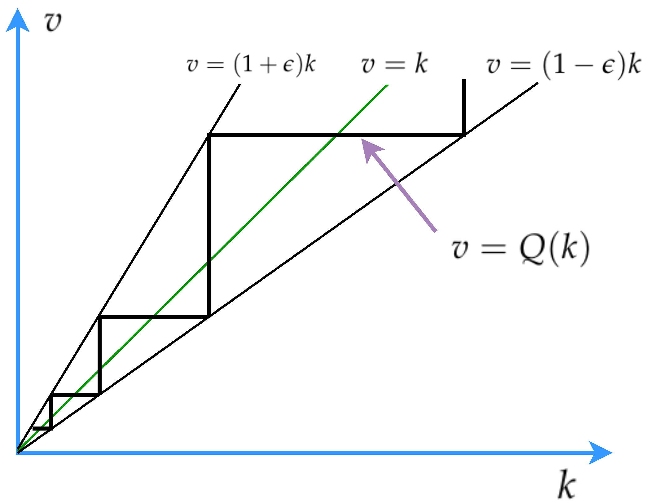
where $\hat{\zeta }\left(t\right)$ stands for the estimation of $\zeta \left(t\right)$, and $\mathcal{K}$ is the estimator gain to be designed. $\mathrm{\Delta }\mathcal{K}$ signifies the fluctuation with ${\mathcal{H}}_k{F}_k\left(t\right){\mathcal{N}}_k,F_k^T\left(t\right)F_k\left(t\right)\le I$. In addition, considering the effect of quantization in [28,29], we introduce the quantitative process to save bandwidth, and the logarithmic quantizer $Q\left(z\right)=\mathrm{col}\left\{Q_1\left(z_1\right),Q_2\left(z_2\right),\cdots ,Q_m\left(z_m\right)\right\}$ is employed (shown in Figure 2). In this paper, $Q\left(z\right)$ is defined as

$$Q_l\left(k_l\right)=\left\{\begin{array}{c}\begin{array}{c}{v}^i{\mu }_0,{\displaystyle \frac{v^i{\mu }_0}{1+ϵ}}<k_l\le {\displaystyle \frac{v^i{\mu }_0}{1-ϵ}},i=0,\pm 1,\pm 2,\cdots \hfill \\ 0, k_l=0,\hfill \\ -Q_l(-k_l),k_l<0\hfill \end{array}\hfill \end{array}\right.$$

(6)

where $v\in (0,1)$ is the quantization density, ${\mu }_0>0$, and $\begin{array}{c}\hfill ϵ={\displaystyle \frac{1-v}{1+v}}\end{array}$.

Analogous to the method in [30], $Q\left(k\right)$ can be described as

$$\begin{array}{c}\hfill \overline{y}\left(t\right)\triangleq Q\left(k\right)=(I+\mathrm{\Delta }\iota )k,\end{array}$$

(7)

where $-ϵ\le \mathrm{\Delta }{\iota }_i\le ϵ$.

Remark 2.

In a network control environment, due to the limitations of bandwidth or bit rate, signals need to be quantized before transmission. A quantizer can be regarded as a device that uses the values in a finite set to convert real-valued data into segmented continuous constant data.

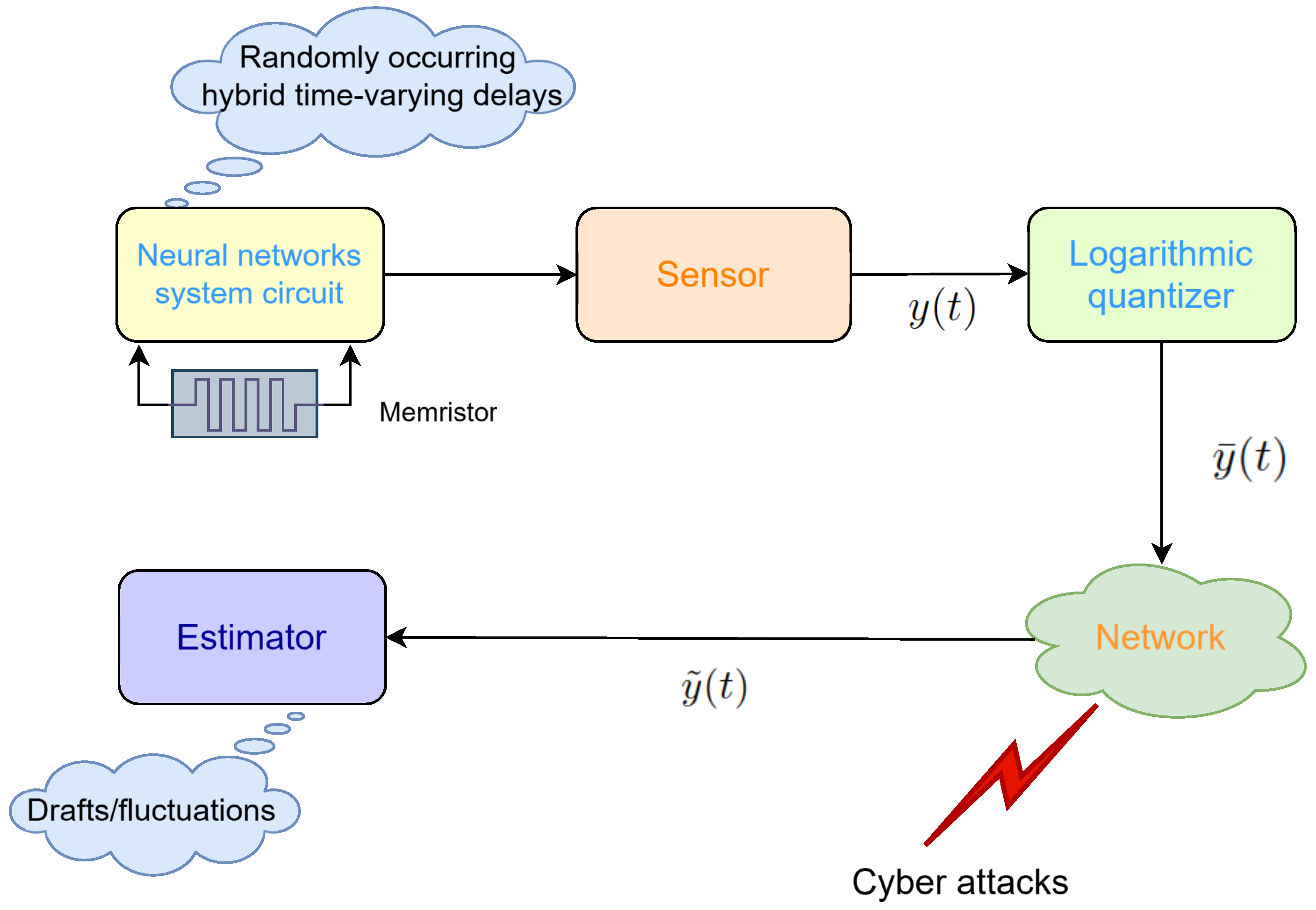
Remark 3.

The flow diagram of memristor-based neural network state estimation is presented in Figure 3. As a circuit system, the synaptic voltage and temporal noise associated with transmitter release must be considered, particularly due to the random occurrence of time delays. In this paper, we utilize the network measurement outputs $y\left(t\right)$ to estimate neural state information. The measurement outputs are transmitted to the network using a logarithmic quantizer. Given the complex network environment, cyber-attacks may occur. When a cyber-attack takes place, the actual data is combined with the attack signal and sent to the state estimator.

The actual input to the state estimator can be described as follows:

$$\begin{array}{c}\hfill \tilde{y}\left(t\right)=(1-\gamma \left(t\right))\overline{y}\left(t\right)+\gamma \left(t\right)g\left(y\left(t\right)\right)\end{array}$$

(8)

where $g(·)$ represents cyber-attacks. $\gamma \left(t\right)$ is used to describe the occurrence probability of stochastic cyber-attacks, and satisfies

$$\begin{array}{c}\hfill \mathrm{Prob}\left\{\gamma \left(t\right)=1\right\}=\mathbb{E}\left\{\gamma \left(t\right)\right\}=\overline{\gamma }.\end{array}$$

Assumption 2.

The nonlinear function $g\left(y\right(t\left)\right)$ satisfies the following condition:

$$\begin{array}{c}\hfill {\parallel g\left(y\left(t\right)\right)\parallel }_2\le {\parallel Gy\left(t\right)\parallel }_2\end{array}$$

(9)

where G is a constant matrix representing the upper bound of the nonlinearity.

Next, denote $r\left(t\right)\triangleq \zeta \left(t\right)-\hat{\zeta }\left(t\right)$, $\tilde{f}\left(r\left(t\right)\right)\triangleq f\left(\zeta \left(t\right)\right)-f\left(\hat{\zeta }\left(t\right)\right)$. Combining (2) and (5)∼(8), the error dynamic can be obtained:

$$\begin{array}{cc}\hfill {}_{t_0}{}^{C}D_t^{\beta }r\left(t\right)=& -\left(\mathcal{C}+\tilde{\mathcal{K}}\mathcal{D}\right)r\left(t\right)+\mathcal{A}\tilde{f}\left(r\left(t\right)\right)+\mathrm{\Delta }\mathcal{A}f\left(\zeta \left(t\right)\right)+\overline{\varrho }\mathcal{B}\tilde{f}\left(r(t-\rho \left(t\right))\right)\hfill \\ \hfill & +\overline{\varrho }\mathrm{\Delta }\mathcal{B}f\left(\zeta (t-\rho \left(t\right))\right)+\overline{\delta }\mathcal{E}{\int }_{t-d\left(t\right)}^t\tilde{f}\left(r\left(s\right)\right)ds+\overline{\delta }\mathrm{\Delta }\mathcal{E}{\int }_{t-d\left(t\right)}^{t}f\left(\zeta \left(s\right)\right)ds\hfill \\ \hfill & +\left(\tilde{\mathcal{K}}\mathcal{D}-\mathrm{\Delta }\mathcal{C}-(1-\gamma \left(t\right))\tilde{\mathcal{K}}\tilde{I}\mathcal{D}\right)\zeta \left(t\right)-\gamma \left(t\right)\tilde{\mathcal{K}}g\left(\mathcal{D}\zeta \left(t\right)\right)+\varsigma \left(t\right),\hfill \end{array}$$

(10)

where

$$\begin{array}{cc}\hfill \varsigma \left(t\right)=& \tilde{\gamma }(\mathcal{B}+\mathrm{\Delta }\mathcal{B})f\left(\zeta (t-\rho \left(t\right))\right)+\tilde{\delta }\left(t\right)(\mathcal{E}+\mathrm{\Delta }\mathcal{E}){\int }_{t-d\left(t\right)}^{t}f\left(\zeta \left(s\right)\right)ds,\hfill \\ \hfill \tilde{\varrho }\left(t\right)=& \varrho \left(t\right)-\overline{\varrho },\tilde{\delta }\left(t\right)=\delta \left(t\right)-\overline{\delta },\tilde{\mathcal{K}}=\mathcal{K}+\mathrm{\Delta }\mathcal{K},\tilde{I}=I+{\mathrm{\Delta }}_{\iota }.\hfill \end{array}$$

Let $\overline{\nu }\left(t\right)\triangleq \mathrm{col}\left\{\zeta \left(t\right),r\left(t\right)\right\}$, ${\phi }_f\left(t\right)\triangleq \mathrm{col}\left\{f\left(t\right),\tilde{f}\left(r\left(t\right)\right)\right\}$, ${\phi }_f(t-\rho \left(t\right))\triangleq \mathrm{col}\left\{f(t-\rho \left(t\right)),\tilde{f}(t-\rho \left(t\right))\right\}$. According to (4) and (10), the augmented system is obtained as

$$\begin{array}{cc}\hfill {}_{t_0}{}^{C}D_t^{\beta }\overline{\nu }\left(t\right)=& -\left(\tilde{\mathcal{C}}+\overrightarrow{\gamma }{\tilde{\mathcal{C}}}_k\right)\overline{\nu }\left(t\right)+\tilde{\mathcal{A}}{\phi }_f\left(t\right)+\overline{\varrho }\tilde{\mathcal{B}}{\phi }_f(t-\rho \left(t\right))-\overline{\gamma }{\tilde{\mathcal{K}}}^{\prime }g\left(\overline{\mathcal{D}}\overline{\nu }\left(t\right)\right)\hfill \\ & +\overline{\delta }\tilde{\mathcal{E}}{\int }_{t-d\left(t\right)}^t{\phi }_f\left(s\right)ds+\tilde{\varsigma }\left(t\right),\hfill \end{array}$$

(11)

where

$$\begin{array}{cc}\hfill \tilde{\mathcal{C}}=& \left[\begin{array}{cc}\mathcal{C}+\mathrm{\Delta }\mathcal{C}& \hat{0}\\ \mathrm{\Delta }\mathcal{C}-\tilde{\mathcal{K}}\mathcal{D}& \mathcal{C}+\tilde{\mathcal{K}}\mathcal{D}\end{array}\right],\tilde{\mathcal{A}}=\left[\begin{array}{cc}\mathcal{A}+\mathrm{\Delta }\mathcal{A}& \hat{0}\\ \mathrm{\Delta }\mathcal{A}& \mathcal{A}\end{array}\right],\overline{\mathcal{D}}={\left[\begin{array}{c}{\mathcal{D}}^T\\ \hat{0}\end{array}\right]}^T,\hfill \\ \hfill \tilde{\mathcal{B}}=& \left[\begin{array}{cc}\mathcal{B}+\mathrm{\Delta }\mathcal{B}& \hat{0}\\ \mathrm{\Delta }\mathcal{B}& \mathcal{B}\end{array}\right],\tilde{\mathcal{E}}=\left[\begin{array}{cc}\mathcal{E}+\mathrm{\Delta }\mathcal{E}& \hat{0}\\ \mathrm{\Delta }\mathcal{E}& \mathcal{E}\end{array}\right],{\tilde{\mathcal{B}}}^{\prime }=\left[\begin{array}{cc}\mathcal{B}+\mathrm{\Delta }\mathcal{B}& \hat{0}\\ \mathcal{B}+\mathrm{\Delta }\mathcal{B}& \hat{0}\end{array}\right],\hfill \\ \hfill {\tilde{\mathcal{E}}}^{\prime }=& \left[\begin{array}{cc}\mathcal{E}+\mathrm{\Delta }\mathcal{E}& \hat{0}\\ \mathcal{E}+\mathrm{\Delta }\mathcal{E}& \hat{0}\end{array}\right],\widetilde{{\mathcal{C}}_k}=\left[\begin{array}{cc}\hat{0}& \hat{0}\\ \tilde{\mathcal{K}}\tilde{I}\mathcal{D}& \hat{0}\end{array}\right],{\tilde{\mathcal{K}}}^{\prime }=\left[\begin{array}{c}\hat{0}\\ \tilde{\mathcal{K}}\end{array}\right],\overrightarrow{\gamma }=1-\overline{\gamma },\hfill \\ \hfill \tilde{\varsigma }\left(t\right)=& \tilde{\gamma }\left(t\right){\tilde{\mathcal{C}}}_k\overline{\nu }\left(t\right)-\tilde{\gamma }\left(t\right){\tilde{\mathcal{K}}}^{\prime }g\left(\overline{\mathcal{D}}\overline{\nu }\left(t\right)\right)+\tilde{\varrho }\left(t\right){\tilde{\mathcal{B}}}^{\prime }{\phi }_f(t-\rho \left(t\right))\hfill \\ & +\tilde{\delta }\left(t\right){\tilde{\mathcal{E}}}^{\prime }{\int }_{t-d\left(t\right)}^t{\phi }_f\left(s\right)ds.\hfill \end{array}$$

Lemma 1

([31]). For the continuous and differential function $\eta \left(t\right)\in {\mathbb{R}}^n$, the following inequation holds:

$$\begin{array}{c}\hfill {}_{t_0}{}^{C}D_t^{\beta }\left({\eta }^T\left(t\right)P\eta \left(t\right)\right)\le 2{\eta }^T\left(t\right)P_{t_0}^C{D}_t^{\beta }\nu \left(t\right),\forall \beta \in (0,1).\end{array}$$

Lemma 2

([32]). For any matrix $\mathcal{O}\in {\mathbb{R}}^{n\times n}$, a vector $\psi :[\rho ,\tau ]\in {\mathbb{R}}^{+}\to {\mathbb{R}}^n$ is differentiable. There exist matrices ${\mathfrak{L}}_1,{\mathfrak{L}}_2\in {\mathbb{R}}^{2n\times n}$ satisfying

$$\begin{array}{cc}\hfill -{}_{\rho }I_{\tau }^{\beta }\left({\psi }^T\left(\tau \right)\mathcal{O}\psi \left(\tau \right)\right)\le & {\zeta }^T(\rho ,\tau )\mathrm{Sym}\left({\mathrm{\Omega }}^{*}\right)\zeta (\rho ,\tau )\hfill \\ & +{\displaystyle \frac{{(\tau -\rho )}^{\beta }}{\mathrm{\Gamma }(\beta +1)}}{\zeta }^T(\rho ,\tau )\mathrm{{\rm Y}}{\hat{\mathcal{O}}}^{-1}{\mathrm{{\rm Y}}}^T\zeta (\rho ,\tau ),\hfill \end{array}$$

where

$$\begin{array}{cc}\hfill \zeta (\rho ,\tau )& =[x^T\left(\rho \right),x^T\left(\tau \right),{\displaystyle \frac{2}{{(\tau -\rho )}^{\beta }}}{}_{\rho }I_{\tau }^{\beta }{x}^T\left(\tau \right){]}^T,\hfill \\ \hfill {\mathrm{\Omega }}^{*}& =N_1{\overline{w}}_1^T+N_2{\overline{w}}_2^T,N_1=I_2-I_1,\psi \left(\tau \right)={}_{\rho }D_{\tau }^{\beta }x\left(\tau \right),\hfill \\ \hfill N_2& ={\displaystyle \frac{1}{\mathrm{\Gamma }\left(\beta \right)}}{I}_3-{\displaystyle \frac{1}{\mathrm{\Gamma }\left(2\beta \right)}}{I}_2+\left({\displaystyle \frac{1}{\mathrm{\Gamma }\left(2\beta \right)}}-{\displaystyle \frac{2}{\mathrm{\Gamma }\left(\beta \right)\mathrm{\Gamma }(\beta +1)}}\right)I_1,\hfill \\ \hfill {\overline{w}}_1& =\left[I_2-I_1,I_3-{\displaystyle \frac{2}{\mathrm{\Gamma }(\beta +1)}}\right]{\mathfrak{L}}_1,{\overline{w}}_2=\left[I_2-I_1,I_3-{\displaystyle \frac{2}{\mathrm{\Gamma }(\beta +1)}}\right]{\mathfrak{L}}_2,\hfill \\ \hfill I_j& ={\left[0_{n(j-1)n},I,0_{n\times (3-j)n}\right]}^T(j=1,2,3),\mathrm{{\rm Y}}=\left[{\overline{w}}_1,{\overline{w}}_2\right],\hfill \\ \hfill \hat{\mathcal{O}}& =\mathrm{diag}\left\{\mathcal{O},3{\mathrm{\Gamma }}^2\left(2\beta \right)\mathcal{O}\right\}.\hfill \end{array}$$

Lemma 3

([33]). For any vector $\zeta \left(t\right):\left[d_1,d_2\right]\to {\mathbb{R}}^n$, a constant matrix $M\in {\mathbb{R}}^{n\times n},M=M^T>0$, two scalars $d_1,d_2(0<d_1<d_2)$. Then, the following inequality is well defined:

$$\begin{array}{c}\hfill (d_2-d_1){\int }_{d_1}^{d_2}{\zeta }^T\left(\tau \right)M\zeta \left(\tau \right)d\tau >{\left({\int }_{d_1}^{d_2}\zeta \left(\tau \right)d\tau \right)}^{T}M\left({\int }_{d_1}^{d_2}\zeta \left(\tau \right)d\tau \right).\end{array}$$

Definition 3

([34]). Consider the fractional-order nonlinear system ${}_{t_0}{}^{C}D^{\beta }\nu \left(t\right)=\mathsf{f}(t,\nu \left(t\right))$. For any scalars $c>0,0<\beta <1$, assume $\mathbb{V}(t,\nu (t\left)\right)$ and the class-$\mathcal{K}$ functions ${\mathfrak{b}}_i(i=1,2,3)$ satisfy

$$\begin{array}{c}\hfill {\mathfrak{b}}_1(\parallel \nu \parallel )\le \mathbb{V}(t,\nu \left(t\right))\le {\mathfrak{b}}_2(\parallel \nu \parallel ),\\ \hfill {}_{t_0}{}^{C}D^{\beta }\mathbb{V}(t,\nu \left(t\right))\le -{\mathfrak{b}}_3(\parallel \nu \parallel )+c{t}^{-\beta }.\end{array}$$

Then, the fractional-order nonlinear system (11) is asymptotically stable.

3. Main Results

In this section, we derive several delay- and order-dependent criteria to ensure the asymptotical stability of the augmented system (11). Several novel Lyapunov–Krasovskii functionals are proposed that incorporate the bounded information of time-varying delays and the order of the system, aiming to reduce conservatism.

For convenience of expression, let

$$\begin{array}{cc}\hfill \overline{\eta }\left(t\right)& ={\left[{\overline{\eta }}_1^T\left(t\right),{\overline{\eta }}_2^T\left(t\right),\cdots ,{\overline{\eta }}_n^T\left(t\right)\right]}^T,{\overline{\eta }}_i\left(t\right)=:{\overline{\nu }}_i\left(t\right)-{}_{t-\rho }I_t^{\beta }{\vartheta }_i\left(t\right),\hfill \\ \hfill \vartheta \left(t\right)& ={\left[{\vartheta }_1^T\left(t\right),{\vartheta }_2^T\left(t\right),\cdots ,{\vartheta }_n^T\left(t\right)\right]}^T,{\vartheta }_i\left(t\right)=-{\displaystyle \frac{1}{\mathrm{\Gamma }(1-\beta )}}{\int }_{t_0}^{t-\rho }{(t-\tau )}^{-\beta }{\dot{\overline{\nu }}}_i\left(\tau \right)d\tau ,\hfill \\ \hfill \tilde{\vartheta }\left(t\right)& =:{\displaystyle \frac{2}{{\rho }^{\beta }}}{}_{t-\rho }I_t^{\beta }\overline{\nu }\left(t\right)-{\displaystyle \frac{2}{{\rho }^{\beta }}}{}_{t-\rho }I_t^{2\beta }\vartheta \left(t\right),\hfill \\ \hfill \varpi \left(t\right)& \triangleq \mathrm{col}\{\overline{\nu }\left(t\right),\overline{\nu }(t-\rho \left(t\right)),\overline{\nu }(t-\rho ),{\phi }_f\left(t\right),{\phi }_f(t-\rho \left(t\right)),{\int }_{t-d\left(t\right)}^t{\phi }_f\left(s\right)ds,\hfill \\ \hfill & g\left(\overline{\mathcal{D}}\overline{\nu }\left(t\right)\right),{}_{t-\rho }I_t^{\beta }\vartheta \left(t\right),\tilde{\vartheta }\left(t\right),{}_{t_0}D_t^{\beta }\overline{\nu }\left(t\right)\},\hfill \\ \hfill {\mathfrak{e}}_i& ={\left[0_{2n\times 2(j-1)n},I_{2n},0_{2n\times 2(10-j)n}\right]}^T,j=1,2,\cdots ,10.\hfill \end{array}$$

Theorem 1.

Let the estimator gain matrix $\mathcal{K}$ and $\mathrm{\Delta }\mathcal{K}$ be given; Assumption 1 holds. For the given positive scalars ρ, $\overline{\gamma }$, $\overline{\varrho }$ and $\overline{\rho }$, the augmented system (11) is stochastically asymptotically stable if there exist positive definite matrices $\mathcal{P}\in {\mathbb{R}}^{2n\times 2n}$, ${\mathcal{Q}}_1\in {\mathbb{R}}^{2n\times 2n}$, ${\mathcal{Q}}_2\in {\mathbb{R}}^{2n\times 2n}$, $\mathcal{O}\in {\mathbb{R}}^{2n\times 2n}$, $M\in {\mathbb{R}}^{4n\times 4n}$, and any matrices $W_1\in {\mathbb{R}}^{4n\times 2n},W_2\in {\mathbb{R}}^{4n\times 2n}$ and scalars ${\kappa }_1>0$, ${\kappa }_2>0$, such that

$$\begin{array}{c}\hfill \tilde{\mathrm{\mho }}=\left[\begin{array}{cc}\mathrm{\mho }& \mathrm{\Xi }\\ ★& -{\displaystyle \frac{\mathrm{\Gamma }(\beta +1)}{{\rho }^{\beta }}}\tilde{\mathcal{Y}}\end{array}\right]<\hat{0},\end{array}$$

(12)

where

$$\begin{array}{cc}\hfill \mathrm{\mho }& ={\mathrm{\Theta }}_1+{\mathrm{\Theta }}_2+{\mathrm{\Pi }}_1+{\mathrm{\Pi }}_2+{\mathrm{{\rm Y}}}_1+{\mathrm{{\rm Y}}}_2+\mathrm{\Lambda }+\mathrm{\Psi }+\mathrm{Sym}\left\{{\mathrm{\aleph }}_1{\mathrm{\Omega }}_1^T+{\mathrm{\aleph }}_2{\mathrm{\Omega }}_2^T\right\},\hfill \\ \hfill {\mathrm{\Theta }}_1& ={\mathfrak{e}}_{10}\mathcal{P}{\mathfrak{e}}_1^T+{\mathfrak{e}}_1\mathcal{P}{\mathfrak{e}}_{11}^T,{\mathrm{\Theta }}_2={\mathfrak{e}}_1{\mathcal{Q}}_1{\mathfrak{e}}_1^T-{\mathfrak{e}}_3{\mathcal{Q}}_2{\mathfrak{e}}_3^T-(1-\overline{\rho }){\mathfrak{e}}_2({\mathcal{Q}}_1-{\mathcal{Q}}_2){\mathfrak{e}}_2^T,\hfill \\ \hfill \tilde{\mathcal{Y}}& =\left[\begin{array}{cc}\mathcal{Y}& 0\\ 0& 3{\mathrm{\Gamma }}^2\left(2\beta \right)\mathcal{Y}\end{array}\right],{\mathrm{\Theta }}_4=\left[\begin{array}{c}{\mathfrak{e}}_1\\ {\mathfrak{e}}_4\end{array}\right]M{\left[\begin{array}{c}{\mathfrak{e}}_1\\ {\mathfrak{e}}_4\end{array}\right]}^T-(1-\overline{\rho })\left[\begin{array}{c}{\mathfrak{e}}_2\\ {\mathfrak{e}}_5\end{array}\right]M{\left[\begin{array}{c}{\mathfrak{e}}_2\\ {\mathfrak{e}}_5\end{array}\right]}^T,\hfill \\ \hfill {\mathrm{\aleph }}_1& ={\mathfrak{e}}_1-{\mathfrak{e}}_8-{\mathfrak{e}}_3,{\mathrm{\aleph }}_2={\displaystyle \frac{{\mathfrak{e}}_8}{\mathrm{\Gamma }\left(\beta \right)}}-{\displaystyle \frac{{\mathfrak{e}}_1-{\mathfrak{e}}_8}{\mathrm{\Gamma }\left(2\beta \right)}}+\left({\displaystyle \frac{1}{\mathrm{\Gamma }\left(2\beta \right)}}-{\displaystyle \frac{2}{\mathrm{\Gamma }\left(\beta \right)\mathrm{\Gamma }(\beta +1)}}\right){\mathfrak{e}}_3,\hfill \\ \hfill {\mathrm{\Omega }}_1& =\left[{\mathfrak{e}}_1-{\mathfrak{e}}_8-{\mathfrak{e}}_3,{\mathfrak{e}}_9-{\displaystyle \frac{2}{\mathrm{\Gamma }(\beta +1)}}{\mathfrak{e}}_3\right]W_1,{\mathrm{\Omega }}_2=\left[{\mathfrak{e}}_1-{\mathfrak{e}}_8-{\mathfrak{e}}_3,{\mathfrak{e}}_9-{\displaystyle \frac{2}{\mathrm{\Gamma }(\beta +1)}}{\mathfrak{e}}_3\right]W_2,\hfill \\ \hfill \mathrm{\Psi }& ={\displaystyle \frac{{\rho }^{\beta }}{\mathrm{\Gamma }(\beta +1)}}{\mathfrak{e}}_{10}\mathcal{Y}{\mathfrak{e}}_{10},{\mathrm{\Pi }}_1=-{\kappa }_1{\mathfrak{e}}_1{J}_1{\mathfrak{e}}_1^T+2{\kappa }_1{\mathfrak{e}}_1{J}_2{\mathfrak{e}}_4^T-{\kappa }_1{\mathfrak{e}}_{4}I{\mathfrak{e}}_4^T,\hfill \\ \hfill \mathrm{\Lambda }& =\mathrm{Sym}\left\{{\mathfrak{e}}_1{\mathcal{W}}_1\Im +{\mathfrak{e}}_{10}{\mathcal{W}}_2\Im \right\},{\mathrm{\Pi }}_2=-{\kappa }_2{\mathfrak{e}}_2{J}_1{\mathfrak{e}}_2^T+2{\kappa }_2{\mathfrak{e}}_2{J}_2{\mathfrak{e}}_5^T-{\kappa }_2{\mathfrak{e}}_{5}I{\mathfrak{e}}_5^T,\hfill \\ \hfill \mathrm{\Xi }& =\left[{\mathrm{\Omega }}_1,{\mathrm{\Omega }}_2\right],{\mathrm{{\rm Y}}}_1={\mathfrak{e}}_1{\overline{\mathcal{D}}}^T{G}^{T}G\overline{\mathcal{D}}{\mathfrak{e}}_1^T-{\mathfrak{e}}_{7}I{\mathfrak{e}}_7^T,{\mathrm{{\rm Y}}}_2=d^2{\mathfrak{e}}_4\mathcal{R}{\mathfrak{e}}_4^T-{\mathfrak{e}}_6\mathcal{R}{\mathfrak{e}}_6^T,\hfill \\ \hfill \Im & =-{\mathfrak{e}}_{10}^T-(\tilde{\mathcal{C}}+\overrightarrow{\gamma }{\tilde{\mathcal{C}}}_k){\mathfrak{e}}_1^T+\tilde{\mathcal{A}}{\mathfrak{e}}_4^T+\overline{\varrho }\tilde{\mathcal{B}}{\mathfrak{e}}_5^T+\overline{\delta }\tilde{\mathcal{E}}{\mathfrak{e}}_6^T-\overline{\gamma }{\tilde{\mathcal{K}}}^{\prime }{\mathfrak{e}}_7^T,\hfill \\ \hfill J_1& =\mathrm{diag}\left\{I\otimes {\displaystyle \frac{{\overrightarrow{F}}_1^T{\overrightarrow{F}}_2+{\overrightarrow{F}}_2^T{\overrightarrow{F}}_1}{2}}\right\},J_2=-\mathrm{diag}\left\{I\otimes {\displaystyle \frac{{\overrightarrow{F}}_1^T+{\overrightarrow{F}}_2^T}{2}}\right\}.\hfill \end{array}$$

Proof. 

Choose the following LKFs:

$$\mathbb{V}(t,\overline{\nu }\left(t\right))=\sum _{h=1}^5{\mathbb{V}}_h(t,\overline{\nu }\left(t\right)),$$

(13)

where

$$\begin{array}{cc}\hfill {\mathbb{V}}_1(t,\overline{\nu }\left(t\right))& ={}_{t_0}{}^{C}D_t^{-(1-\beta )}\left(\overline{\nu }{\left(t\right)}^T\mathcal{P}\overline{\nu }\left(t\right)\right),\hfill \\ \hfill {\mathbb{V}}_2(t,\overline{\nu }\left(t\right))& ={\int }_{t-\rho \left(t\right)}^t{\eta }_0^T\left(\tau \right)M{\eta }_0\left(\tau \right)d\tau ,\hfill \\ \hfill {\mathbb{V}}_3(t,\overline{\nu }\left(t\right))& ={\int }_{t-\rho \left(t\right)}^t{\overline{\nu }}^T\left(\tau \right){\mathcal{Q}}_1\overline{\nu }\left(\tau \right)d\tau +{\int }_{t-\rho }^{t-\rho \left(t\right)}{\overline{\nu }}^T\left(\tau \right){\mathcal{Q}}_2\overline{\nu }\left(\tau \right)d\tau ,\hfill \\ \hfill {\mathbb{V}}_4(t,\overline{\nu }\left(t\right))& ={\displaystyle \frac{1}{\mathrm{\Gamma }\left(\beta \right)}}{\int }_{-\rho }^0{\left(-\theta \right)}^{\beta -1}{\int }_{t+\theta }^t{V}^{*}\left(\tau \right)d\tau d\theta ,\hfill \\ \hfill {\mathbb{V}}_5(t,\overline{\nu }\left(t\right))& =d{\int }_{-d}^0{\int }_{t+\theta }^t{\left({\phi }_f\left(\tau \right)\right)}^T\mathcal{R}{\phi }_f\left(\tau \right)d\tau d\theta .\hfill \end{array}$$

with ${\eta }_0\left(t\right)\triangleq {\left[{\overline{\nu }}^T\left(t\right),{\phi }_f^T\left(t\right)\right]}^T,V^{*}\left(t\right)={\left({}_{t_0}{}^{C}D_t^{\beta }\overline{\nu }\left(t\right)\right)}^T\mathcal{Y}\left({}_{t_0}{}^{C}D_t^{\beta }\overline{\nu }\left(t\right)\right)$.

Define the infinitesimal operator $\mathcal{L}$ of $\mathbb{V}(t,\overline{\nu }\left(t\right))$ [35] as follows:

$$\begin{array}{c}\hfill \mathcal{L}\mathbb{V}(t,\overline{\nu }\left(t\right))=\underset{\epsilon \to 0^{+}}{lim}{\displaystyle \frac{1}{\epsilon }}\left\{\mathbb{E}\left\{\mathbb{V}(t+\epsilon ,\overline{\nu }(t+\epsilon )){|}_{(t,\overline{\nu }\left(t\right))}\right\}-\mathbb{V}(t,\overline{\nu }\left(t\right))\right\}.\end{array}$$

According to Lemma 1,

$$\begin{array}{cc}\hfill \mathbb{E}\left\{\mathcal{L}{\mathbb{V}}_1(t,\overline{\nu }\left(t\right))\right\}\le & \mathbb{E}\{{\left({}_{t_0}{}^{C}D_t^{\beta }\overline{\nu }\left(t\right)\right)}^T\mathcal{P}\overline{\nu }\left(t\right)+{\overline{\nu }}^T\left(t\right)\mathcal{P}{}_{t_0}{}^{C}D_t^{\beta }\overline{\nu }\left(t\right)\hfill \\ & +{\displaystyle \frac{{\overline{\nu }}^T\left(t_0\right)\mathcal{P}\overline{\nu }\left(t_0\right)}{\mathrm{\Gamma }(1-\beta )}}{t}^{-\beta }\},\hfill \end{array}$$

(14)

$$\begin{array}{cc}\hfill \mathbb{E}\left\{\mathcal{L}{\mathbb{V}}_2(t,\overline{\nu }\left(t\right))\right\}=& \mathbb{E}\left\{{\eta }_0^T\left(t\right)M{\eta }_0\left(t\right)-(1-\dot{\rho }\left(t\right)){\eta }_0^T(t-\rho \left(t\right))M{\eta }_0(t-\rho \left(t\right))\right\}\hfill \\ \hfill \le & \mathbb{E}\left\{{\eta }_0^T\left(t\right)M{\eta }_0\left(t\right)-(1-\overline{\rho }){\eta }_0^T(t-\rho \left(t\right))M{\eta }_0(t-\rho \left(t\right))\right\},\hfill \end{array}$$

(15)

$$\begin{array}{cc}\hfill \mathbb{E}\left\{\mathcal{L}{\mathbb{V}}_3(t,\overline{\nu }\left(t\right))\right\}=& \mathbb{E}\{{\overline{\nu }}^T\left(t\right){\mathcal{Q}}_1\overline{\nu }\left(t\right)-{\overline{\nu }}^T(t-\rho ){\mathcal{Q}}_2\overline{\nu }(t-\rho )\hfill \\ & -(1-\dot{\rho }\left(t\right)){\overline{\nu }}^T(t-\rho \left(t\right))\left({\mathcal{Q}}_1-{\mathcal{Q}}_2\right)\overline{\nu }(t-\rho \left(t\right))\}\hfill \\ \hfill \le & \mathbb{E}\{{\overline{\nu }}^T\left(t\right){\mathcal{Q}}_1\overline{\nu }\left(t\right)-{\overline{\nu }}^T(t-\rho ){\mathcal{Q}}_2\overline{\nu }(t-\rho )\hfill \\ & -(1-\overline{\rho }){\overline{\nu }}^T(t-\rho \left(t\right))\left({\mathcal{Q}}_1-{\mathcal{Q}}_2\right)\overline{\nu }(t-\rho \left(t\right))\}.\hfill \end{array}$$

(16)

As stated by Lemma 2, one has

$$\begin{array}{cc}\hfill & \mathbb{E}\left\{\mathcal{L}{\mathbb{V}}_4(t,\overline{\nu }\left(t\right))\right\}\hfill \\ \hfill =& \mathbb{E}\{{\displaystyle \frac{1}{\mathrm{\Gamma }\left(\beta \right)}}{\int }_{-\rho }^0{(-\theta )}^{\beta -1}{\left({}_{t_0}{}^{C}D_t^{\beta }\overline{\nu }\left(t\right)\right)}^T\mathcal{Y}\left({}_{t_0}{}^{C}D_t^{\beta }\overline{\nu }\left(t\right)\right)d\theta \hfill \\ & -{\displaystyle \frac{1}{\mathrm{\Gamma }\left(\beta \right)}}{\int }_{-\rho }^0{(-\theta )}^{\beta -1}{\left({}_{t_0}{}^{C}D_{t+\theta }^{\beta }\overline{\nu }(t+\theta )\right)}^T\mathcal{Y}\left({}_{t_0}{}^{C}D_{t+\theta }^{\beta }\overline{\nu }(t+\theta )\right)d\theta \}\hfill \\ \hfill =& \mathbb{E}\{{\displaystyle \frac{{\rho }^{\beta }}{\mathrm{\Gamma }(\beta +1)}}{\left({}_{t_0}{}^{C}D_t^{\beta }\overline{\nu }\left(t\right)\right)}^T\mathcal{Y}\left({}_{t_0}{}^{C}D_t^{\beta }\overline{\nu }\left(t\right)\right)\hfill \\ \hfill & -{\displaystyle \frac{1}{\mathrm{\Gamma }\left(\beta \right)}}{\int }_{t-\rho }^t{\left(t-\mu \right)}^{\beta -1}{\left({}_{t_0}{}^{C}D_{\mu }^{\beta }\overline{\nu }\left(\mu \right)\right)}^T\mathcal{Y}\left({}_{t_0}{}^{C}D_{\mu }^{\beta }\overline{\nu }\left(\mu \right)\right)d\mu \}.\hfill \end{array}$$

(17)

In accordance with the Definition 1 and Lemma 2, one gets

$$\begin{array}{cc}\hfill & -{\displaystyle \frac{1}{\mathrm{\Gamma }\left(\beta \right)}}{\int }_{t-\rho }^t{\left(t-\mu \right)}^{\beta -1}{\left({}_{t_0}{}^{C}D_{\mu }^{\beta }\overline{\nu }\left(\mu \right)\right)}^T\mathcal{Y}\left({}_{t_0}{}^{C}D_{\mu }^{\beta }\overline{\nu }\left(\mu \right)\right)d\mu \hfill \\ \hfill =& -{\displaystyle \frac{1}{\mathrm{\Gamma }\left(\beta \right)}}{\int }_{t-\rho }^t{\left(t-\mu \right)}^{\beta -1}{\left({}_{t-\rho }D_{\mu }^{\beta }\overline{\eta }\left(\mu \right)\right)}^T\mathcal{Y}\left({}_{t-\rho }D_{\mu }^{\beta }\overline{\eta }\left(\mu \right)\right)d\mu \hfill \\ \hfill \le & {\varpi }^T\left(t\right){\displaystyle \frac{\mathrm{{\rm Y}}{\tilde{\mathcal{Y}}}^{-1}{\mathrm{{\rm Y}}}^T}{\mathrm{\Gamma }(\beta +1){\rho }^{-\beta }}}\varpi \left(t\right)+{\varpi }^T\left(t\right)\mathrm{Sym}\left\{{\mathrm{\aleph }}_1{\mathrm{{\rm Y}}}_1^T+{\mathrm{\aleph }}_2{\mathrm{{\rm Y}}}_2^T\right\}\varpi \left(t\right).\hfill \end{array}$$

(18)

On the basis of Lemma 3, we have

$$\begin{array}{cc}\hfill \mathbb{E}\left\{\mathcal{L}{\mathbb{V}}_5(t,\overline{\nu }\left(t\right))\right\}& =\mathbb{E}\left\{d{\int }_{-d}^0{\phi }_f^T\left(\tau \right)\mathcal{R}{\phi }_f\left(\tau \right)d\tau -d{\int }_{-d}^0{\phi }_f^T(t+\tau )\mathcal{R}{\phi }_f(t+\tau )d\tau \right\}\hfill \\ & =\mathbb{E}\left\{d^2{\phi }_f^T\left(t\right)\mathcal{R}{\phi }_f\left(t\right)-d{\int }_{t-d}^t{\phi }_f^T\left(\tau \right)\mathcal{R}{\phi }_f\left(\tau \right)d\tau \right\}\hfill \\ & \le \mathbb{E}\left\{d^2{\phi }_f^T\left(t\right)\mathcal{R}{\phi }_f\left(t\right)-{\int }_{t-d\left(t\right)}^t{\phi }_f^T\left(\tau \right)d\tau \mathcal{R}{\int }_{t-d\left(t\right)}^t{\phi }_f\left(\tau \right)d\tau \right\}.\hfill \end{array}$$

(19)

According to the Assumption 1, the following inequation can be inferred:

$$\begin{array}{c}\hfill {\left[\begin{array}{c}\overline{\nu }\left(t\right)\\ {\phi }_f\left(t\right)\end{array}\right]}^T\left[\begin{array}{cc}{J}_1& J_2\\ \ast & I\end{array}\right]\left[\begin{array}{c}\overline{\nu }\left(t\right)\\ {\phi }_f\left(t\right)\end{array}\right]\le \hat{0},\end{array}$$

(20)

$$\begin{array}{c}\hfill {\left[\begin{array}{c}\overline{\nu }(t-\rho \left(t\right))\\ {\phi }_f(t-\rho \left(t\right))\end{array}\right]}^T\left[\begin{array}{cc}{J}_1& J_2\\ \ast & I\end{array}\right]\left[\begin{array}{c}\overline{\nu }(t-\rho \left(t\right))\\ {\phi }_f(t-\rho \left(t\right))\end{array}\right]\le \hat{0}.\end{array}$$

(21)

  From Assumption (2), which is the limited condition of cyber-attacks, we can get

$$\begin{array}{c}\hfill {\overline{\nu }}^T\left(t\right){\overline{\mathcal{D}}}^T{G}^{T}G\overline{\mathcal{D}}\overline{\nu }\left(t\right)-g^T\left(\overline{\mathcal{D}}\overline{\nu }\left(t\right)\right)g\left(\overline{\mathcal{D}}\overline{\nu }\left(t\right)\right)\ge \hat{0}\end{array}$$

(22)

For any matrices ${\mathcal{W}}_1$ and ${\mathcal{W}}_2$, integrating the augmented system (11), we have

$$\begin{array}{cc}\hfill \hat{0}=& \mathbb{E}\left\{2\left[{\overline{\nu }}^T\left(t\right){\mathcal{W}}_1+{}_{t_0}{}^{C}D_t^{\beta }{\overline{\nu }}^T\left(t\right){\mathcal{W}}_2\right]\right[-{}_{t_0}{}^{C}D_t^{\beta }\overline{\nu }\left(t\right)-\left(\tilde{\mathcal{C}}+\overrightarrow{\gamma }\widetilde{{\mathcal{C}}_k}\right)\overline{\nu }\left(t\right)+\tilde{\mathcal{A}}{\phi }_f\left(t\right)\hfill \\ & +\overline{\varrho }\tilde{\mathcal{B}}{\phi }_f(t-\rho \left(t\right))+\overline{\delta }\tilde{\mathcal{E}}{\int }_{t-d\left(t\right)}^t{\phi }_f\left(s\right)ds-\overline{\gamma }{\tilde{\mathcal{K}}}^{\prime }g\left(\overline{\mathcal{D}}\overline{\nu }\left(t\right)\right)+\tilde{\varsigma }\left(t\right)\left]\right\}.\hfill \end{array}$$

(23)

Combining (14)∼(23), when (12) holds, one gets

$$\begin{array}{cc}\hfill \mathbb{E}\left\{\mathcal{L}\mathbb{V}(t,\overline{\nu }\left(t\right))\right\}\le & \mathbb{E}\left\{{\varpi }^T\left(t\right)\left(\mathrm{\mho }+{\displaystyle \frac{{\rho }^{\beta }}{\mathrm{\Gamma }(\beta +1)}}\mathrm{\Xi }{\tilde{\mathcal{Y}}}^{-1}{\mathrm{\Xi }}^T\right)\varpi \left(t\right)+{\displaystyle \frac{{\overline{\nu }}^T\left(t_0\right)\mathcal{P}\overline{\nu }\left(t_0\right)}{\mathrm{\Gamma }(1-\beta )}}{t}^{-\beta }\right\}\hfill \\ \hfill \le & {\lambda }_{min}\left(\tilde{\mathrm{\mho }}\right){\overline{\nu }}^T\left(t\right)\overline{\nu }\left(t\right)+{\displaystyle \frac{{\overline{\nu }}^T\left(t_0\right)\mathcal{P}\overline{\nu }\left(t_0\right)}{\mathrm{\Gamma }(1-\beta )}}{t}^{-\beta }.\hfill \end{array}$$

(24)

According to Definition 3, it can be inferred that $\underset{t\to \infty }{lim}{\parallel \mathbb{E}\left\{\overline{\nu }\left(t\right)\right\}\parallel }^2=0$. Then, the augmented system (11) is stochastically asymptotically stable.    □

Remark 4.

So far, numerous excellent results regarding the stability of delayed FONNs can be obtained [7,15,26,29,36,37]. However, most of these significant findings are delay-independent. The stability criterion proposed in this paper depends not only on the time-varying delay information, but also on the system order β. This is to say, by adjusting the bounded information of time-varying delays and the order β of the neural network systems, the feasible domain of the stability criterion can be effectively improved and have less conservatism.

In what follows, the estimator design for the memristor-based FONNs (1) based on the conclusion of Theorem 1 will be detailed.

Theorem 2.

For given positive sclars ρ, $\overline{\gamma }$, $\overline{\varrho }$, and $\overline{\rho }$, the augmented system (11) is stochastically asymptotically stable if there exist positive definite matrices $\mathcal{P}\in {\mathbb{R}}^{2n\times 2n}$, ${\mathcal{Q}}_1\in {\mathbb{R}}^{2n\times 2n}$, ${\mathcal{Q}}_2\in {\mathbb{R}}^{2n\times 2n}$, $\mathcal{O}\in {\mathbb{R}}^{2n\times 2n}$, $M\in {\mathbb{R}}^{4n\times 4n}$, and any matrices $W_1\in {\mathbb{R}}^{4n\times 2n},W_2\in {\mathbb{R}}^{4n\times 2n}$,$\mathcal{W}=\mathrm{diag}\left\{V_1,V_2\right\}$ and scalars ${\kappa }_1>0$, ${\kappa }_2>0$, $\mathfrak{u}>0,\mathfrak{t}>0,\mathfrak{s}>0$ and $\mathfrak{r}>0$ satisfying the following LMIs:

$$\begin{array}{c}\hfill \left[\begin{array}{ccc}{\overline{\mathrm{\mho }}}^{\prime }& \mathrm{\Xi }& {\overrightarrow{ð}}_1\\ ★& -{\displaystyle \frac{\mathrm{\Gamma }(\beta +1)}{{\rho }^{\beta }}}\tilde{\mathcal{Y}}& \hat{0}\\ ★& ★& -{\overrightarrow{ð}}_2\end{array}\right]<\hat{0},\end{array}$$

(25)

where

$$\begin{array}{cc}\hfill {\overline{\mathrm{\mho }}}^{\prime }& ={\mathrm{\Theta }}_1+{\mathrm{\Theta }}_2+{\mathrm{\Pi }}_1+{\mathrm{\Pi }}_2+{\mathrm{{\rm Y}}}_1+{\mathrm{{\rm Y}}}_2+\mathrm{\Psi }+\mathrm{Sym}\left\{{\mathrm{\aleph }}_1{\mathrm{\Omega }}_1^T+{\mathrm{\aleph }}_2{\mathrm{\Omega }}_2^T\right\}+{\overline{\mathrm{\Lambda }}}^{\prime },\hfill \\ \hfill {\overline{\mathrm{\Lambda }}}^{\prime }& =\mathrm{Sym}\{-{\mathfrak{e}}_1\mathcal{W}{\mathfrak{e}}_{10}^T-{\mathfrak{e}}_1\overrightarrow{\mathcal{C}}{\mathfrak{e}}_1^T-\overrightarrow{\gamma }{\mathfrak{e}}_1{\overrightarrow{\mathcal{C}}}_k{\mathfrak{e}}_1^T+{\mathfrak{e}}_1\overline{\mathcal{A}}{\mathfrak{e}}_4^T+\overline{\varrho }{\mathfrak{e}}_1\mathcal{W}\overline{\mathcal{B}}{\mathfrak{e}}_5^T+\overline{\delta }{\mathfrak{e}}_1\mathcal{W}\overline{\mathcal{E}}{\mathfrak{e}}_6^T\hfill \\ & -\overline{\gamma }{\mathcal{e}}_1{\overrightarrow{\mathcal{K}}}^{\prime }{\mathfrak{e}}_7^T-\tilde{\mu }{\mathfrak{e}}_{10}\mathcal{W}{\mathfrak{e}}_{10}^T-\tilde{\mu }{\mathfrak{e}}_{10}\overrightarrow{\mathcal{C}}{\mathfrak{e}}_1^T-\tilde{\mu }\overrightarrow{\gamma }{\mathfrak{e}}_{10}{\overrightarrow{\mathcal{C}}}_k{\mathfrak{e}}_1^T+\tilde{\mu }{\mathfrak{e}}_{10}\overline{\mathcal{A}}{\mathfrak{e}}_4^T+\tilde{\mu }\overline{\varrho }{\mathfrak{e}}_{10}\mathcal{W}\overline{\mathcal{B}}{\mathfrak{e}}_5^T\hfill \\ & +\tilde{\mu }\overline{\delta }{\mathfrak{e}}_{10}\mathcal{W}\overline{\mathcal{E}}{\mathfrak{e}}_6^T-\tilde{\mu }\overline{\gamma }{\mathfrak{e}}_{10}{\overrightarrow{\mathcal{K}}}^{\prime }{\mathfrak{e}}_7^T\},\hfill \\ \hfill {\overrightarrow{ð}}_1& =\left[\overrightarrow{\gamma }\mathcal{ϝ}{\overrightarrow{\mathcal{K}}}^{\prime },ϵ\mathfrak{u}{\mathcal{e}}_1{\overline{N}}_d^T,\mathcal{ϝ}\mathcal{W}{\tilde{H}}_k,ϵ\mathfrak{t}{\mathfrak{e}}_1{\overline{N}}_k^T,\tilde{\mathcal{H}},\mathfrak{r}{\tilde{\mathcal{N}}}^T,\mathcal{ϝ}{\tilde{\mathcal{H}}}_k,\mathfrak{s}{\tilde{\mathcal{N}}}_k^T\right],\tilde{\mathfrak{s}}=\mathrm{diag}\left\{\mathfrak{s},\mathfrak{s}\right\},\hfill \\ \hfill {\overrightarrow{ð}}_2& =\mathrm{diag}\left\{\tilde{\mathfrak{u}}I,\tilde{\mathfrak{t}}I,\tilde{\mathfrak{r}}I,\tilde{\mathfrak{s}}I\right\},\tilde{\mathfrak{u}}=\mathrm{diag}\left\{\mathfrak{u},\mathfrak{u}\right\},\tilde{\mathfrak{t}}=\mathrm{diag}\left\{\mathfrak{t},\mathfrak{t}\right\},\tilde{\mathfrak{r}}=\mathrm{diag}\left\{\mathfrak{r},\mathfrak{r}\right\},\hfill \\ \hfill {\overrightarrow{\mathcal{C}}}_k& =\left[\begin{array}{cc}\hat{0}& \hat{0}\\ -\mathcal{X}\mathcal{D}& \hat{0}\end{array}\right],\overrightarrow{\mathcal{C}}=\left[\begin{array}{cc}{V}_1\mathcal{C}& \hat{0}\\ -\mathcal{X}\mathcal{D}& V_2\mathcal{C}+\mathcal{X}\mathcal{D},\end{array}\right],{\overrightarrow{\mathcal{K}}}^{\prime }=\left[\begin{array}{c}\hat{0}\\ \mathcal{X}\end{array}\right].\hfill \end{array}$$

Other terms ${\mathrm{\Theta }}_j$, ${\mathrm{\Pi }}_j$, ${\mathrm{{\rm Y}}}_j(j=1,2)$, $\mathrm{\Psi }$, $\tilde{\mathcal{Y}}$, $\mathrm{\Xi }$ have been defined in Theorem 1. If $(\mathcal{P}$, ${\mathcal{Q}}_1$, ${\mathcal{Q}}_2$, $\mathcal{O}$, $\mathcal{R}$, $\mathcal{W}$, $\mathfrak{u}$, $\mathfrak{t}$, $\mathfrak{s}$, $\mathfrak{r}$, ${\kappa }_1$, ${\kappa }_2)$ are a set of feasible solutions of (25), Algorithm 1 shows the process of calculating the developed estimator gain $\mathcal{K}$. Then, the estimator gain matrix $\mathcal{K}$ in (5) can be designed as

$$\begin{array}{c}\hfill \mathcal{K}=V_2^{-1}\mathcal{X}.\end{array}$$

(26)

Algorithm 1 Estimator Gain $\mathcal{K}$

Step i:   Supply the system parameters for memristor-based FONNs (1) and (5). Step ii:  Set the constants $\overline{\rho },d,\overline{\delta },\rho$ Step iii: By means of the Matlab LMI Toolbox and the parameters in Step i and ii, seek the feasible solution of (25). If the feasible solutions can not find, return to Step i and ii and reset the correlation parameters. Step iv: According to the feasible solutions and the setting $\mathcal{X}=V_2\mathcal{K}$, calculate the estimator gain $\mathcal{K}$.

Proof. 

First, define $X\left(t\right)\triangleq {\left[{\overline{\nu }}^T\left(t\right){\left(t_0{D}_t^{\beta }\overline{\nu }\left(t\right)\right)}^T\right]}^T,\mathcal{W}=\mathrm{diag}\left\{V_1,V_2\right\}$, in which $\mathcal{W}={\mathcal{W}}_1$, ${\mathcal{W}}_2=\tilde{\mu }\mathcal{W}(\tilde{\mu }>0)$ and $\mathcal{W}$ is a non-singular matrix. Then, (23) can be rewritten as

$$\begin{array}{cc}\hfill \hat{0}=& \mathbb{E}\left\{2X^T\left(t\right)\mathcal{W}\right[-{}_{t_0}{}^{C}D_t^{\beta }\overline{\nu }\left(t\right)-\left(\overline{\mathcal{C}}+\overrightarrow{\gamma }{\overline{\mathcal{C}}}_k\right)\overline{\nu }\left(t\right)+\overline{\mathcal{A}}{\phi }_f\left(t\right)+\overline{\varrho }\overline{\mathcal{B}}{\phi }_f(t-\rho \left(t\right))\hfill \\ & +\overline{\delta }\overline{\mathcal{E}}{\int }_{t-d\left(t\right)}^t{\phi }_f\left(s\right)ds-{\tilde{H}}_k{F}_k\left(t\right){\tilde{N}}_k\overline{\nu }\left(t\right)-\overline{\gamma }{\overline{\mathcal{K}}}^{\prime }g\left(\overline{\mathcal{D}}\overline{\nu }\left(t\right)\right)+\tilde{\varsigma }\left(t\right)\hfill \\ & -\overrightarrow{\gamma }{\tilde{H}}_k{F}_k\left(t\right){\overline{N}}_k\overline{\nu }\left(t\right)+\tilde{H}{\tilde{F}}_a\left(t\right){\tilde{N}}_a{\phi }_f\left(t\right)+\tilde{H}{\tilde{F}}_b\left(t\right){\tilde{N}}_b{\phi }_f(t-\rho \left(t\right))\hfill \\ \hfill & -\overline{\gamma }{\tilde{H}}_k{F}_k\left(t\right){\mathcal{N}}_{k}g\left(\overline{\mathcal{D}}\overline{\nu }\left(t\right)\right)-\overrightarrow{\gamma }{\overrightarrow{H}}_k{\mathrm{\Delta }}_{\iota }{\overline{N}}_d\overline{\nu }\left(t\right)-\overrightarrow{\gamma }{\tilde{H}}_k{F}_k\left(t\right){\mathrm{\Delta }}_{\iota }{\overline{N}}_k\overline{\nu }\left(t\right)\left]\right\},\hfill \end{array}$$

(27)

where

$$\begin{array}{cc}\hfill \overline{\mathcal{C}}& =\left[\begin{array}{cc}\mathcal{C}& 0\\ -\mathcal{K}\mathcal{D}& \mathcal{C}+\mathcal{K}\mathcal{D}\end{array}\right],{\overline{\mathcal{C}}}_k=\left[\begin{array}{cc}0& 0\\ \mathcal{K}\mathcal{D}& 0\end{array}\right],\overline{\mathcal{A}}=\left[\begin{array}{cc}\mathcal{A}& 0\\ 0& \mathcal{A}\end{array}\right],{\tilde{H}}_k=\left[\begin{array}{c}0\\ {\mathcal{H}}_k\end{array}\right],\hfill \\ \hfill \overline{\mathcal{B}}& =\left[\begin{array}{cc}\mathcal{B}& 0\\ 0& \mathcal{B}\end{array}\right],\overline{\mathcal{E}}=\left[\begin{array}{cc}\mathcal{E}& 0\\ 0& \mathcal{E}\end{array}\right],\tilde{H}=\left[\begin{array}{cc}H& 0\\ 0& H\end{array}\right],{\tilde{N}}_a=\left[\begin{array}{cc}{N}_a& 0\\ N_a& 0\end{array}\right],{\overrightarrow{H}}_k=\left[\begin{array}{c}0\\ \mathcal{K}\end{array}\right],\hfill \\ \hfill {\tilde{N}}_b& =\left[\begin{array}{cc}\overline{\varrho }{N}_b& 0\\ \overline{\varrho }{N}_b& 0\end{array}\right],{\tilde{N}}_c=\left[\begin{array}{cc}-N_c& 0\\ -N_c& 0\end{array}\right],{\tilde{N}}_e=\left[\begin{array}{cc}\overline{\delta }{N}_e& 0\\ \overline{\delta }{N}_e& 0\end{array}\right],{\overline{N}}_k=\left[{\mathcal{N}}_k\mathcal{D},0\right],\hfill \\ \hfill {\tilde{F}}_a\left(t\right)& =\mathrm{diag}\left\{F_a\left(t\right),F_a\left(t\right)\right\},{\tilde{F}}_b\left(t\right)=\mathrm{diag}\left\{F_b\left(t\right),F_b\left(t\right)\right\},{\tilde{N}}_k=\left[-{\mathcal{N}}_k\mathcal{D},{\mathcal{N}}_k\mathcal{D}\right],\hfill \\ \hfill {\tilde{F}}_c\left(t\right)& =\mathrm{diag}\left\{F_c\left(t\right),F_c\left(t\right)\right\},{\tilde{F}}_e\left(t\right)=\mathrm{diag}\left\{F_e\left(t\right),F_e\left(t\right)\right\},{\overline{N}}_d=\left[-\mathcal{D},0\right].\hfill \end{array}$$

In order to eliminate the uncertainties $\mathrm{\Delta }\mathcal{C}$, $\mathrm{\Delta }\mathcal{A}$, $\mathrm{\Delta }\mathcal{B}$, and $\mathrm{\Delta }\mathcal{E}$ in (12), the inequation $\pm 2\mathfrak{a}\mathfrak{b}\le \sigma {\mathfrak{a}}^T\mathfrak{a}+{\sigma }^{-1}{\mathfrak{b}}^T\mathfrak{b}$ is utilized, and there exists an arbitrary scalar $\mathfrak{r}>0$ satisfying

$$\begin{array}{cc}\hfill & 2\mathcal{ϝ}\mathcal{W}\left[\tilde{H}{\tilde{F}}_c\left(t\right){\tilde{N}}_c{\mathfrak{e}}_1^T+\tilde{H}{\tilde{F}}_a\left(t\right){\tilde{N}}_a{\mathfrak{e}}_4^T+\tilde{H}{\tilde{F}}_b\left(t\right){\tilde{N}}_b{\mathfrak{e}}_5^T+\tilde{H}{\tilde{F}}_e\left(t\right){\tilde{N}}_e{\mathfrak{e}}_6^T\right]\hfill \\ \hfill =& \tilde{\mathcal{H}}\tilde{\mathcal{F}}\left(t\right)\tilde{\mathcal{N}}\le {\mathfrak{r}}^{-1}\tilde{\mathcal{H}}{\tilde{\mathcal{H}}}^T+\mathfrak{r}{\tilde{\mathcal{N}}}^T\tilde{\mathcal{N}},\hfill \end{array}$$

(28)

$$\begin{array}{cc}\hfill & 2\mathcal{ϝ}\mathcal{W}\left[-{\tilde{H}}_k{F}_k\left(t\right){\tilde{N}}_k{\mathfrak{e}}_1^T-\overrightarrow{\gamma }{\tilde{H}}_k{F}_k\left(t\right){\overrightarrow{N}}_k{\mathfrak{e}}_1^T-\overline{\gamma }{\tilde{H}}_k{F}_k\left(t\right){\mathcal{N}}_k{\mathfrak{e}}_7^T\right]\hfill \\ \hfill =& {\tilde{H}}_k{F}_k\left(t\right){\tilde{\mathcal{N}}}_k\le {\mathfrak{s}}^{-1}{\tilde{\mathcal{H}}}_k{\tilde{\mathcal{H}}}_k^T+\mathfrak{s}{\tilde{\mathcal{N}}}_k^T{\tilde{\mathcal{N}}}_k,\hfill \end{array}$$

(29)

where

$$\begin{array}{cc}\hfill \tilde{\mathcal{F}}\left(t\right)& =\mathrm{diag}\left\{{\tilde{F}}_c\left(t\right),{\tilde{F}}_a\left(t\right),{\tilde{F}}_b\left(t\right),{\tilde{F}}_e\left(t\right)\right\},\mathcal{ϝ}={\mathfrak{e}}_1+\tilde{\mu }{\mathfrak{e}}_{10},\hfill \\ \hfill \tilde{\mathcal{H}}& =\left[\begin{array}{cccc}\mathcal{W}\tilde{H}& \cdots & \cdots & \mathcal{W}\tilde{H}\\ \hat{0}& \cdots & \cdots & \hat{0}\\ \tilde{\mu }\mathcal{W}\tilde{H}& \cdots & \cdots & \tilde{\mu }\mathcal{W}\tilde{H}\end{array}\right],\tilde{\mathcal{N}}=\left[\begin{array}{cccccc}{\tilde{N}}_c& \hat{0}& \hat{0}& \hat{0}& \hat{0}& \hat{0}\\ \hat{0}& \hat{0}& {\tilde{N}}_a& \hat{0}& \hat{0}& \hat{0}\\ \hat{0}& \hat{0}& \hat{0}& {\tilde{N}}_b& \hat{0}& \hat{0}\\ \hat{0}& \hat{0}& \hat{0}& \hat{0}& {\tilde{N}}_e& \hat{0}\end{array}\right],\hfill \\ \hfill {\tilde{\mathcal{N}}}_k& =\left[-{\tilde{N}}_k-\overrightarrow{\gamma }{\overline{N}}_k,\hat{0},\hat{0},\hat{0},-\overline{\gamma }{\mathcal{N}}_k,\hat{0}\right].\hfill \end{array}$$

Similarly to (28), for the arbitrary scalars $\mathfrak{u}$ and $\mathfrak{t}$, one has

$$\begin{array}{cc}\hfill -2\overrightarrow{\gamma }\mathcal{ϝ}\mathcal{W}{\overrightarrow{H}}_k{\mathrm{\Delta }}_{\iota }{\overline{N}}_d{\mathfrak{e}}_1^T\le {\overrightarrow{\gamma }}^2{\mathfrak{u}}^{-1}\mathcal{ϝ}\mathcal{W}{\overrightarrow{H}}_k{\overrightarrow{H}}_k^T{\mathcal{ϝ}}^T+{ϵ}^2\mathfrak{u}{\mathfrak{e}}_1{\overline{N}}_d^T{\overline{N}}_d{\mathfrak{e}}_1^T,& \end{array}$$

(30)

$$\begin{array}{cc}\hfill -2\mathcal{ϝ}\mathcal{W}{\tilde{H}}_k{F}_k\left(t\right){\mathrm{\Delta }}_{\iota }{\overline{N}}_k{\mathfrak{e}}_1^T\le {\mathfrak{t}}^{-1}\mathcal{ϝ}\mathcal{W}{\tilde{H}}_k{\tilde{H}}_k^T\mathcal{W}{\mathcal{ϝ}}^T+{ϵ}^2\mathfrak{t}{\mathfrak{e}}_1{\overline{N}}_k^T{\overline{N}}_k{\mathfrak{e}}_1^T,& \hfill \end{array}$$

(31)

Combining (12) and (27)∼(31), we can get

$$\begin{array}{cc}\hfill \tilde{\mathrm{\mho }}\le & \overline{\mathrm{\mho }}+{\mathfrak{r}}^{-1}\tilde{\mathcal{H}}{\tilde{\mathcal{H}}}^T+\mathfrak{r}{\tilde{\mathcal{N}}}^T\tilde{\mathcal{N}}+{\overrightarrow{\gamma }}^2{\mathfrak{u}}^{-1}\mathcal{ϝ}\mathcal{W}{\overrightarrow{H}}_k{\overrightarrow{H}}_k^T{\mathcal{ϝ}}^T+{\mathfrak{s}}^{-1}{\tilde{\mathcal{H}}}_k{\tilde{\mathcal{H}}}_k^T\hfill \\ \hfill & +\mathfrak{s}{\tilde{\mathcal{N}}}_k^T{\tilde{\mathcal{N}}}_k+{ϵ}^2\mathfrak{u}{\mathfrak{e}}_1{\overline{N}}_d^T{\overline{N}}_d{\mathfrak{e}}_1^T+{\mathfrak{t}}^{-1}\mathcal{ϝ}\mathcal{W}{\tilde{H}}_k{\tilde{H}}_k^T\mathcal{W}{\mathcal{ϝ}}^T\hfill \\ \hfill & +{ϵ}^2\mathfrak{t}{\mathfrak{e}}_1{\overline{N}}_k^T{\overline{N}}_k{\mathfrak{e}}_1^T+{\displaystyle \frac{{\rho }^{\beta }}{\mathrm{\Gamma }(\beta +1)}}\mathrm{\Xi }{\tilde{\mathcal{O}}}^{-1}{\mathrm{\Xi }}^T\hfill \\ \hfill <& \hat{0},\hfill \end{array}$$

(32)

in which $\overline{\mathrm{\mho }}={\mathrm{\Theta }}_1+{\mathrm{\Theta }}_2+{\mathrm{{\rm Y}}}_1+{\mathrm{{\rm Y}}}_2+{\mathrm{\Pi }}_1+{\mathrm{\Pi }}_2+\mathrm{\Psi }+\mathrm{Sym}\left\{{\mathrm{\aleph }}_1{\mathrm{\Omega }}_1^T+{\mathrm{\aleph }}_2{\mathrm{\Omega }}_2^T\right\}+\overline{\mathrm{\Lambda }}$,

$$\begin{array}{cc}\hfill \overline{\mathrm{\Lambda }}& =\mathrm{Sym}\{-\mathcal{ϝ}\mathcal{W}{\mathfrak{e}}_{10}^T-\mathcal{ϝ}\mathcal{W}(\overline{\mathcal{C}}+\overrightarrow{\gamma }{\overline{\mathcal{C}}}_k){\mathfrak{e}}_1^T+\mathcal{ϝ}\mathcal{W}\overline{\mathcal{A}}{\mathfrak{e}}_4^T+\overline{\varrho }\mathcal{ϝ}\mathcal{W}\overline{\mathcal{B}}{\mathfrak{e}}_5^T\hfill \\ \hfill & +\overline{\delta }\mathcal{ϝ}\mathcal{W}\overline{\mathcal{E}}{\mathfrak{e}}_6^T-\overline{\gamma }\mathcal{ϝ}\mathcal{W}{\overline{\mathcal{K}}}^{\prime }{\mathfrak{e}}_7^T\}.\hfill \end{array}$$

The other terms ${\mathrm{\Theta }}_1$, ${\mathrm{\Theta }}_2$, ${\mathrm{{\rm Y}}}_1$, ${\mathrm{{\rm Y}}}_2$, ${\mathrm{\Pi }}_1$, $\mathrm{\Psi }$ and ${\mathrm{\Pi }}_2$ have been defined in Theorem 1.

To facilitate the calculation of the estimator gain $\mathcal{K}$, the variable $\mathcal{X}=V_2\mathcal{K}$ is defined. When Equation (32) is satisfied, it can be deduced from Schur’s Lemma that Equation (25) holds. From this, it can be known that the augmented system (11) is asymptotically stable. The proof is completed. □

Next, ignoring the random-occurrence characteristics of time-varying delays in (1), the memristor-based FONNs (1) are simplified to a type of traditional FONN with hybrid time-varying delays. In an ideal environment, the following fractional-order state estimator with ideal gain is designed:

$$\left\{\begin{array}{c}\begin{array}{cc}\hfill {}_{t_0}{}^{C}D_t^{\beta }\hat{\zeta }\left(t\right)=& -\mathcal{C}\hat{\zeta }\left(t\right)+\mathcal{A}f\left(\hat{\zeta }\left(t\right)\right)+\mathcal{B}f\left(\hat{\zeta }(t-\rho \left(t\right))\right)+\mathcal{E}{\int }_{t-d\left(t\right)}^{t}f\left(\hat{\zeta }\left(s\right)\right)ds\hfill \\ & +{\mathcal{K}}^{\prime }(y\left(t\right)-\hat{y}\left(t\right)),\hfill \\ \hfill \hat{y}\left(t\right)=& \mathcal{D}\hat{\zeta }\left(t\right),\hfill \end{array}\hfill \end{array}\right.$$

(33)

The following Corollary 1 can be easily inferred from Theorem 2. Therefore, the proof is omitted.

Corollary 1.

Under Assumption 1, for given scalars ρ, $\overline{\rho }$, the augmented system (11) is stochastically asymptotically stable if there exist positive symmetric matrices $\mathcal{P}\in {\mathbb{R}}^{2n\times 2n}$, ${\mathcal{Q}}_1\in {\mathbb{R}}^{2n\times 2n}$, ${\mathcal{Q}}_2\in {\mathbb{R}}^{2n\times 2n}$, $\mathcal{O}\in {\mathbb{R}}^{2n\times 2n}$, $M\in {\mathbb{R}}^{4n\times 4n}$, any matrices $W_1\in {\mathbb{R}}^{4n\times 2n},W_2\in {\mathbb{R}}^{4n\times 2n},\mathcal{W}=\mathrm{diag}\left\{V_1,V_2\right\}$, scalars ${\kappa }_1>0$, ${\kappa }_2>0$, $\mathfrak{r}>0$ satisfying the following LMI:

$$\begin{array}{c}\hfill \left[\begin{array}{cccc}{\overline{\mathrm{\mho }}}^{\prime \prime }& \mathrm{\Xi }& \tilde{\mathcal{H}}& \mathfrak{r}{\tilde{\mathcal{N}}}^{\prime }\\ ★& -{\displaystyle \frac{\mathrm{\Gamma }(\beta +1)}{{\rho }^{\beta }}}\tilde{\mathcal{Y}}& \hat{0}& \hat{0}\\ ★& ★& -\mathfrak{r}I& \hat{0}\\ ★& ★& ★& -\mathfrak{r}I\end{array}\right]<\hat{0},\end{array}$$

(34)

where

$$\begin{array}{cc}\hfill {\overline{\mathrm{\mho }}}^{\prime \prime }& ={\mathrm{\Theta }}_1+{\mathrm{\Theta }}_2+{\mathrm{\Pi }}_1+{\mathrm{\Pi }}_2+{\mathrm{{\rm Y}}}_1+{\mathrm{{\rm Y}}}_2+\mathrm{\Psi }+\mathrm{Sym}\left\{{\mathrm{\aleph }}_1{\mathrm{\Omega }}_1^T+{\mathrm{\aleph }}_2{\mathrm{\Omega }}_2^T\right\}+{\overline{\mathrm{\Lambda }}}^{\prime \prime },\hfill \\ \hfill {\overline{\mathrm{\Lambda }}}^{\prime \prime }& =\mathrm{Sym}\{-{\mathfrak{e}}_1\mathcal{W}{\mathfrak{e}}_{10}^T-{\mathfrak{e}}_1\overrightarrow{\mathcal{C}}{\mathfrak{e}}_1^T-\overrightarrow{\gamma }{\mathfrak{e}}_1{\overrightarrow{\mathcal{C}}}_k{\mathfrak{e}}_1^T+{\mathfrak{e}}_1\overline{\mathcal{A}}{\mathfrak{e}}_4^T+{\mathfrak{e}}_1\mathcal{W}\overline{\mathcal{B}}{\mathfrak{e}}_5^T+{\mathfrak{e}}_1\mathcal{W}\overline{\mathcal{E}}{\mathfrak{e}}_6^T\hfill \\ & -{\overline{\gamma }}_1{\overrightarrow{\mathcal{K}}}^{\prime }{\mathfrak{e}}_7^T-\tilde{\mu }{\mathfrak{e}}_{10}\mathcal{W}{\mathfrak{e}}_{10}^T-\tilde{\mu }{\mathfrak{e}}_{10}\overrightarrow{\mathcal{C}}{\mathfrak{e}}_1^T-\tilde{\mu }\overrightarrow{\gamma }{\mathfrak{e}}_{10}{\overrightarrow{\mathcal{C}}}_k{\mathfrak{e}}_1^T+\tilde{\mu }{\mathfrak{e}}_{10}\overline{\mathcal{A}}{\mathfrak{e}}_4^T+\tilde{\mu }{\mathfrak{e}}_{10}\mathcal{W}\overline{\mathcal{B}}{\mathfrak{e}}_5^T\hfill \\ & +\tilde{\mu }{\mathfrak{e}}_{10}\mathcal{W}\overline{\mathcal{E}}{\mathfrak{e}}_6^T-\tilde{\mu }\overline{\gamma }{\mathcal{e}}_{10}{\overrightarrow{\mathcal{K}}}^{\prime }{\mathfrak{e}}_7^T\},\hfill \\ \hfill {\tilde{\mathcal{N}}}^{\prime }& =\left[\begin{array}{cc}{\tilde{N}}_1& \hat{0}\\ \hat{0}& {\tilde{N}}_2\end{array}\right],{\tilde{N}}_1=\left[\begin{array}{ccc}{\tilde{N}}_c& \hat{0}& \hat{0}\\ \hat{0}& \hat{0}& {\tilde{N}}_a\end{array}\right],{\tilde{N}}_2=\left[\begin{array}{ccc}{\tilde{N}}_b^{\prime }& \hat{0}& \hat{0}\\ \hat{0}& {\tilde{N}}_e^{\prime }& \hat{0}\end{array}\right],\hfill \\ \hfill {\tilde{N}}_b^{\prime }& =\left[\begin{array}{cc}{N}_b& \hat{0}\\ N_b& \hat{0}\end{array}\right],{\tilde{N}}_e^{\prime }=\left[\begin{array}{cc}{N}_e& \hat{0}\\ N_e& \hat{0}\end{array}\right].\hfill \end{array}$$

The rest terms ${\mathrm{\Theta }}_1$, ${\mathrm{\Theta }}_2$, ${\mathrm{{\rm Y}}}_1$, ${\mathrm{{\rm Y}}}_2$, $\mathrm{\Psi }$, ${\mathrm{\Pi }}_1$, ${\mathrm{\Pi }}_2$ can be found in Theorem 2. The estimator gain matrix ${\mathcal{K}}^{\prime }$ is calculated by ${\mathcal{K}}^{\prime }=V_2^{-1}\mathcal{X}$.

Based on the Corollary 1, a further discussion is carried out. Denote $c_{ij}^{\prime }=c_{ij}^{\prime \prime }$, $a_{ij}^{\prime }=a_{ij}^{\prime \prime }$, $b_{ij}^{\prime }=b_{ij}^{\prime \prime }$, $e_{ij}^{\prime }=e_{ij}^{\prime \prime }$. The fractional-order memristive neural networks (1) are simplified to a class of traditional FONNs with mixed delays. In an ideal environment, the following Corollary 2 can be obtained. This criterion can be directly derived from Corollary 1.

Corollary 2.

Suppose that Assumption 1, and let scalars ρ, $\overline{\rho }$, be given; if there exist positive definite matrices $\mathcal{P}\in {\mathbb{R}}^{2n\times 2n}$, ${\mathcal{Q}}_1\in {\mathbb{R}}^{2n\times 2n}$, ${\mathcal{Q}}_2\in {\mathbb{R}}^{2n\times 2n}$, $\mathcal{O}\in {\mathbb{R}}^{2n\times 2n}$, $M\in {\mathbb{R}}^{4n\times 4n}$, any diagonal matrix $\mathcal{W}=\mathrm{diag}\left\{V_1,V_2\right\}$, and scalars ${\kappa }_1>0$, ${\kappa }_2>0$ satisfying the following LMI:

$$\begin{array}{c}\hfill \left[\begin{array}{cc}{\overline{\mathrm{\mho }}}^{\prime \prime }& \mathrm{\Xi }\\ ★& -{\displaystyle \frac{\mathrm{\Gamma }(\beta +1)}{{\rho }^{\beta }}}\tilde{\mathcal{Y}}\end{array}\right]<\hat{0},\end{array}$$

(35)

then, the augmented estimation error system (11) is asymptotically stable, where, ${\overline{\mathrm{\mho }}}^{\prime \prime }$, $\mathrm{\Xi }$, and $\tilde{\mathcal{Y}}$ have been defined in Corollary 1. The estimator gain ${\mathcal{K}}^{\prime }$ is computed by ${\mathcal{K}}^{\prime \prime }=V_2^{-1}\mathcal{X}$.

Remark 5.

In this paper, several novel LKFs containing the integral term $\begin{array}{c}\hfill {\int }_{t-\rho }^t{}_{t_0}{}^{C}D_{\tau }^{\beta }{\overline{\nu }}^T\left(\tau \right)\mathcal{Y}{}_{t_0}{}^{C}D_t^{\beta }\overline{\nu }\left(\tau \right)d\tau \end{array}$ and time delay information are constructed. Combining fractional-order Lyapunov approaches and a novel free-matrix-based integral inequality, several delay and order-dependent criteria are derived to guarantee the existence of a nonfragile state estimator. In [32,36,38], the available results are delay-independent or contain less time delay information. The results in this paper are delay- and order-independent, which reduces conservatism.

4. Numerical Examples

Numerical simulation examples are provided in this section to verify the validity and superiority of the aforementioned theoretical results.

Example 1.

To verify the validity of the estimator method in this paper, consider a class of 2-D fractional-order memristive neural network models (1):

$$\left\{\begin{array}{c}\begin{array}{cc}\hfill {}_{t_0}{}^{C}D^{\beta }{\zeta }_1\left(t\right)=& -c_1\left({\zeta }_1\left(t\right)\right){\zeta }_1\left(t\right)+a_{11}\left({\zeta }_1\left(t\right)\right)f_1\left({\zeta }_1\left(t\right)\right)+a_{12}\left({\zeta }_1\left(t\right)\right)f_2\left({\zeta }_2\left(t\right)\right)\hfill \\ & +\varrho \left(t\right)b_{11}\left({\zeta }_1\left(t\right)\right)f_1\left({\zeta }_1(t-\rho \left(t\right))\right)+\varrho \left(t\right)b_{12}\left({\zeta }_1\left(t\right)\right){\mathsf{f}}_2\left({\zeta }_2(t-\rho \left(t\right))\right)\hfill \\ & +\delta \left(t\right)e_{11}\left({\zeta }_1\left(t\right)\right){\int }_{t-d\left(t\right)}^t{f}_1\left({\zeta }_1\left(s\right)\right)ds+\delta \left(t\right)e_{12}\left({\zeta }_1\left(t\right)\right){\int }_{t-d\left(t\right)}^t{f}_2\left({\zeta }_2\left(s\right)\right)ds,\hfill \\ \hfill {}_{t_0}{}^{C}D^{\beta }{\zeta }_2\left(t\right)=& -c_2\left({\zeta }_2\left(t\right)\right){\zeta }_2\left(t\right)+a_{21}\left({\zeta }_2\left(t\right)\right)f_1\left({\zeta }_1\left(t\right)\right)+a_{22}\left({\zeta }_2\left(t\right)\right)f_2\left({\zeta }_2\left(t\right)\right)\hfill \\ & +\varrho \left(t\right)b_{21}\left({\zeta }_2\left(t\right)\right)f_1\left({\zeta }_1(t-\rho \left(t\right))\right)+\varrho \left(t\right)b_{22}\left({\zeta }_2\left(t\right)\right){\mathsf{f}}_2\left({\zeta }_2(t-\rho \left(t\right))\right)\hfill \\ & +\delta \left(t\right)e_{21}\left({\zeta }_2\left(t\right)\right){\int }_{t-d\left(t\right)}^t{f}_1\left({\zeta }_1\left(s\right)\right)ds+\delta \left(t\right)e_{22}\left({\zeta }_2\left(t\right)\right){\int }_{t-d\left(t\right)}^t{f}_2\left({\zeta }_2\left(s\right)\right)ds,\hfill \end{array}\hfill \end{array}\right.$$

(36)

where the correspond parameters can be chosen as

$$\begin{array}{cc}\hfill a_{11}\left({\zeta }_1(·)\right)& =\left\{\begin{array}{c}-0.59,|{\zeta }_1(·)|\le 1,\hfill \\ -0.60,|{\zeta }_1(·)|>1,\hfill \end{array}\right.\hspace{1em}{a}_{12}\left({\zeta }_1(·)\right)=\left\{\begin{array}{c}1.00,|{\zeta }_1(·)|\le 1,\hfill \\ 0.50,|{\zeta }_1(·)|>1,\hfill \end{array}\right.\hfill \\ \hfill a_{21}\left({\zeta }_2(·)\right)& =\left\{\begin{array}{c}0.20,|{\zeta }_2(·)|\le 1,\hfill \\ -0.70,|{\zeta }_2(·)|>1,\hfill \end{array}\right.\hspace{1em}{a}_{22}\left({\zeta }_2(·)\right)=\left\{\begin{array}{c}-0.82,|{\zeta }_2(·)|\le 1,\hfill \\ -0.50,|{\zeta }_2(·)|>1,\hfill \end{array}\right.\hfill \\ \hfill b_{11}\left({\zeta }_1(·)\right)& =\left\{\begin{array}{c}0.60,|{\zeta }_1(·)|\le 1,\hfill \\ 1.20,|{\zeta }_1(·)|>1,\hfill \end{array}\right.\hspace{1em}{b}_{12}\left({\zeta }_1(·)\right)=\left\{\begin{array}{c}0.05,|{\zeta }_1(·)|\le 1,\hfill \\ -0.25,|{\zeta }_1(·)|>1,\hfill \end{array}\right.\hfill \\ \hfill b_{21}\left({\zeta }_2(·)\right)& =\left\{\begin{array}{c}0.30,|{\zeta }_2(·)|\le 1,\hfill \\ -0.70,|{\zeta }_2(·)|>1,\hfill \end{array}\right.\hspace{1em}{b}_{22}\left({\zeta }_2(·)\right)=\left\{\begin{array}{c}-0.10,|{\zeta }_2(·)|\le 1,\hfill \\ -0.40,|{\zeta }_2(·)|>1,\hfill \end{array}\right.\hfill \\ \hfill e_{11}\left({\zeta }_1(·)\right)& =\left\{\begin{array}{c}-0.70,|{\zeta }_1(·)|\le 1,\hfill \\ -0.80,|{\zeta }_1(·)|>1,\hfill \end{array}\right.\hspace{1em}{e}_{12}\left({\zeta }_1(·)\right)=\left\{\begin{array}{c}0.25,|{\zeta }_1(·)|\le 1,\hfill \\ 0.15,|{\zeta }_1(·)|>1,\hfill \end{array}\right.\hfill \\ \hfill e_{21}\left({\zeta }_2(·)\right)& =\left\{\begin{array}{c}0.30,|{\zeta }_2(·)|\le 1,\hfill \\ -1.00,|{\zeta }_2(·)|>1,\hfill \end{array}\right.\hspace{1em}{e}_{22}\left({\zeta }_2(·)\right)=\left\{\begin{array}{c}-0.70,|{\zeta }_2(·)|\le 1,\hfill \\ -0.40,|{\zeta }_2(·)|>1,\hfill \end{array}\right.\hfill \\ \hfill c_{11}\left({\zeta }_1(·)\right)& =\left\{\begin{array}{c}0.70,|{\zeta }_1(·)|\le 1,\hfill \\ 0.90,|{\zeta }_1(·)|>1,\hfill \end{array}\right.\hspace{1em}{c}_{22}\left({\zeta }_2(·)\right)=\left\{\begin{array}{c}0.85,|{\zeta }_2(·)|\le 1,\hfill \\ 1.00,|{\zeta }_2(·)|>1,\hfill \end{array}\right.\hfill \end{array}$$

then, one can derive that

$$\begin{array}{cc}\hfill \mathcal{A}=& \left[\begin{array}{cc}-0.75& 0.75\\ -0.25& -0.65\end{array}\right],\mathcal{B}=\left[\begin{array}{cc}0.90& -0.10\\ -0.20& -0.25\end{array}\right],\mathcal{E}=\left[\begin{array}{cc}-0.75& 0.2\\ -0.35& -0.55\end{array}\right],\hfill \\ \hfill N_a=& \left[\begin{array}{cccc}0.15& 0.25& 0& 0\\ 0& 0& 0.45& 0.15\end{array}\right],N_b=\left[\begin{array}{cccc}0.30& 0.15& 0& 0\\ 0& 0& 0.50& 0.15\end{array}\right],\hfill \\ \hfill N_e=& \left[\begin{array}{cccc}0.05& 0.05& 0& 0\\ 0& 0& 0.65& 0.15\end{array}\right],N_c=\left[\begin{array}{cccc}0.100& 0& 0& 0\\ 0& 0& 0& 0.075\end{array}\right],\hfill \\ \hfill \mathcal{D}=& \left[\begin{array}{cc}-0.1& 0.3\\ 0& -0.4\end{array}\right],{\mathcal{H}}_k=\left[\begin{array}{cc}0.1& 0\\ 0& 0.1\end{array}\right],{\mathcal{N}}_k=\left[\begin{array}{cc}0.4& 0.4\\ 0.4& 0.4\end{array}\right].\hfill \end{array}$$

The time-varying delays $\rho \left(t\right)$ and $d\left(t\right)$ are chosen as $\rho \left(t\right)=0.02+0.4|sin(t\left)\right|$, $d\left(t\right)=0.05+0.3|cos(t\left)\right|$, which imply $\rho =0.42$, $\overline{\rho }=0.4$, $d=0.35$.

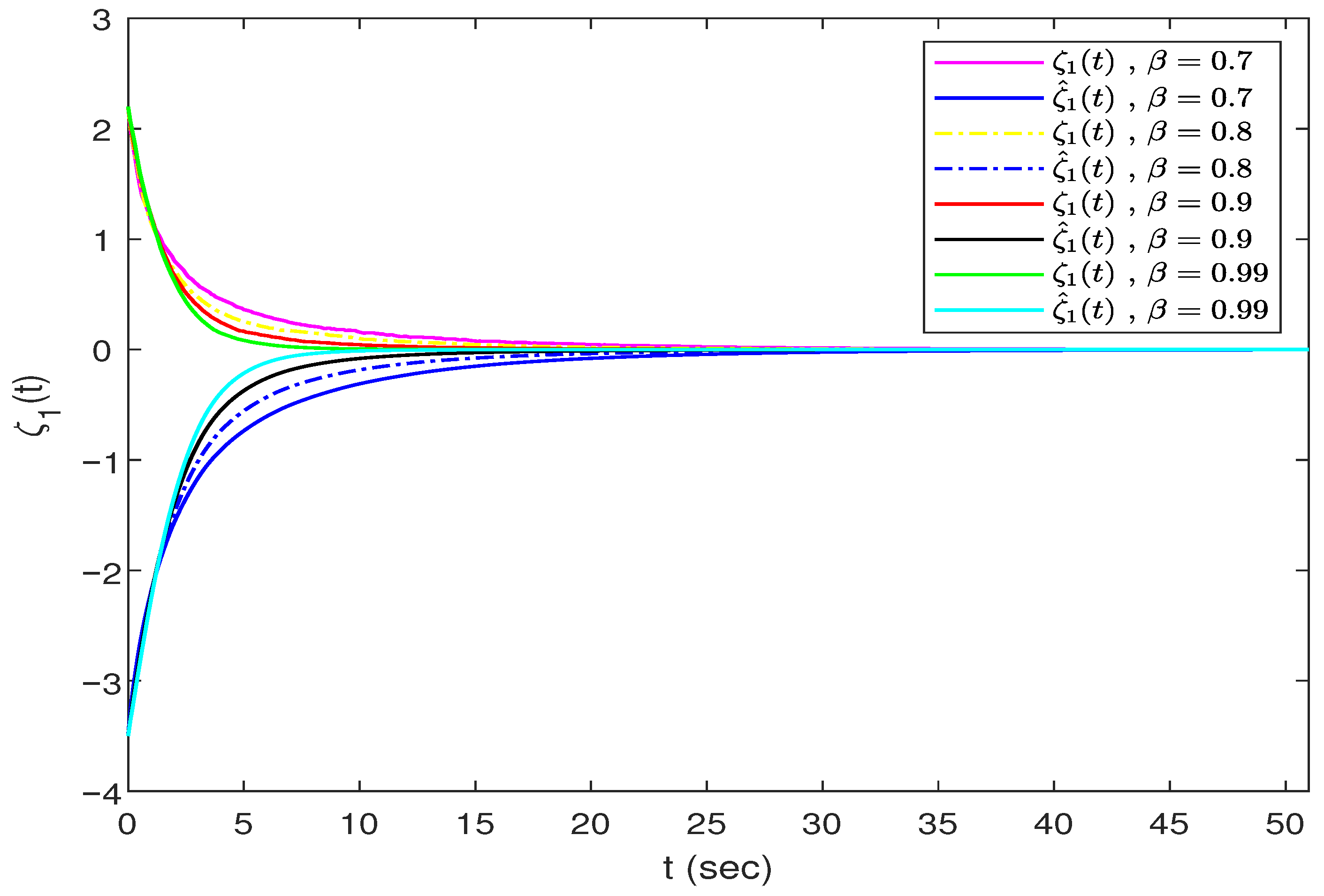
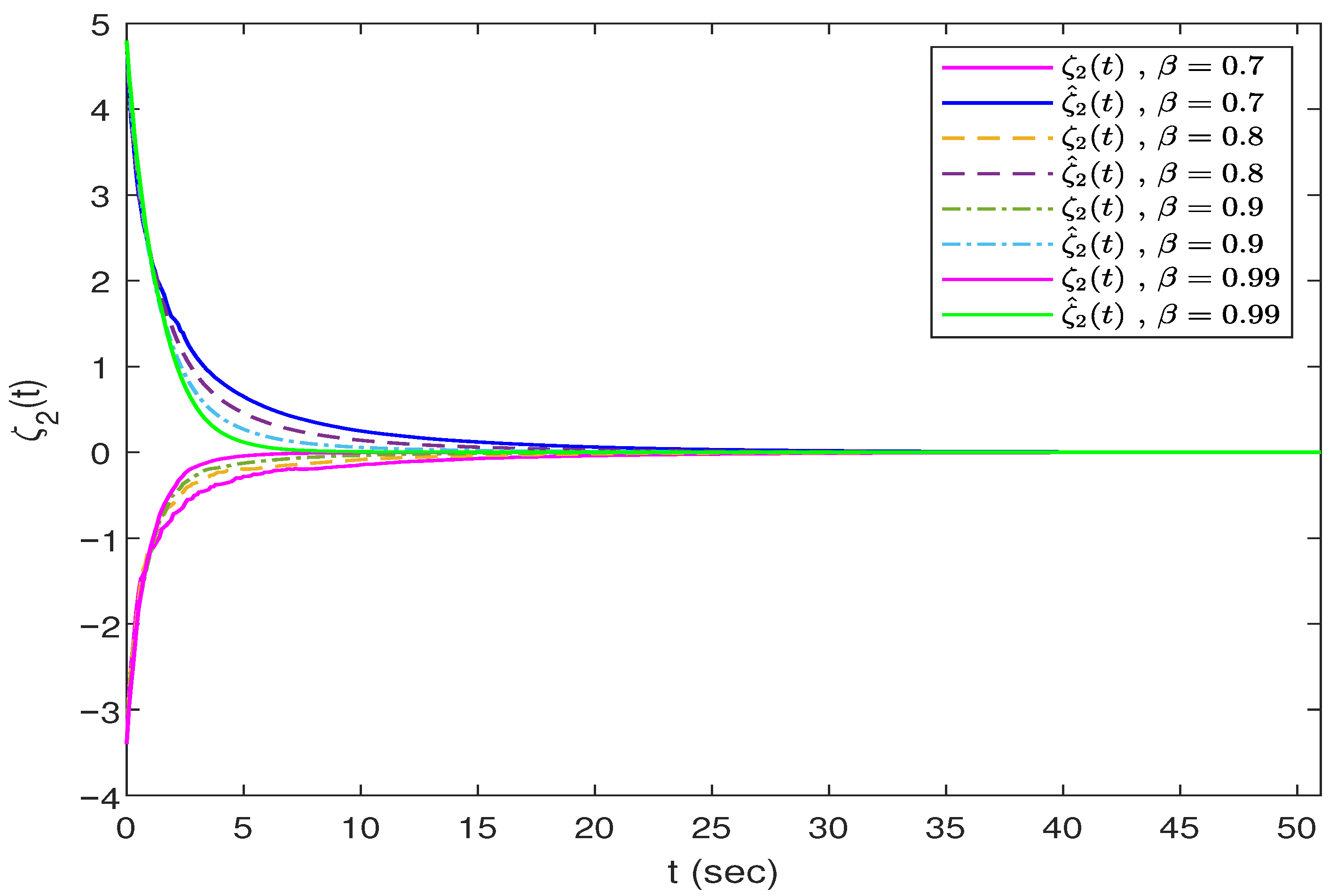
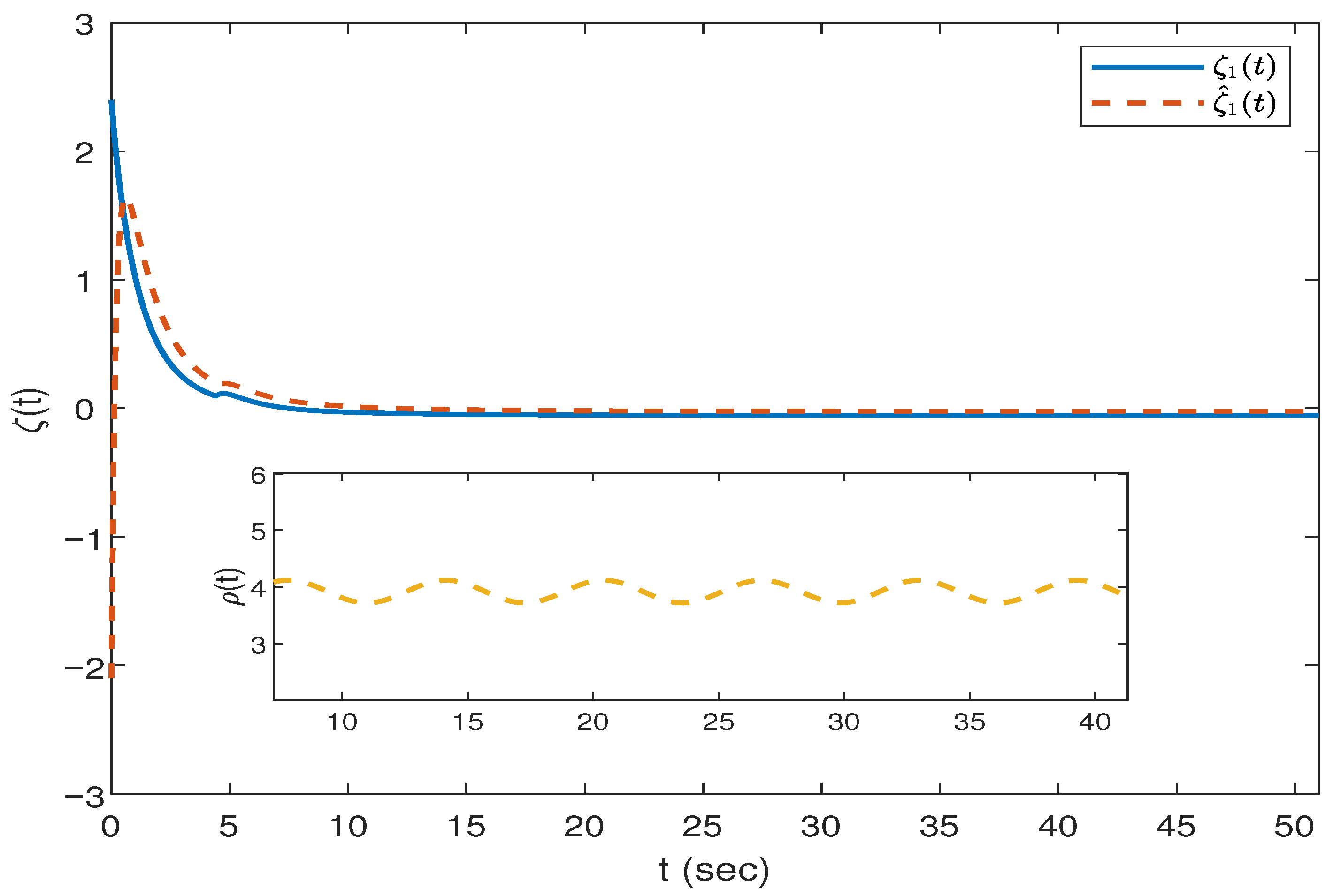
In this example, we assume that the time-varying delays $\rho \left(t\right)$ and $d\left(t\right)$ satisfy $\overline{\varrho }=\mathbb{E}\left\{\varrho \left(t\right)\right\}=0.7$, $\overline{\delta }=\mathbb{E}\left\{\delta \left(t\right)\right\}=0.65$. Choose the following activation functions:

$$f\left(\zeta \left(t\right)\right)=\left[\begin{array}{c}-0.4{\zeta }_1\left(t\right)+\tanh \left(0.2{\zeta }_1\left(t\right)\right)+0.3{\zeta }_2\left(t\right)\\ -0.2{\zeta }_2\left(t\right)+\tanh \left(0.3{\zeta }_2\left(t\right)\right)\end{array}\right],$$

which implies that

$${\overrightarrow{F}}_1=\left[\begin{array}{cc}-0.4& 0.3\\ 0& -0.2\end{array}\right],{\overrightarrow{F}}_2=\left[\begin{array}{cc}-0.2& 0.3\\ 0& 0.1\end{array}\right].$$

By utilizing the Matlab LMI Toolbox, we can obtain a set of solutions of LMIs (25) as follows:

$$\begin{array}{c}\hfill U_2=\left[\begin{array}{cc}0.0409& 0.0013\\ 0.0013& 0.0384\end{array}\right],\mathcal{X}=\left[\begin{array}{cc}0.0046& -0.0029\\ -0.0025& 0.0048\end{array}\right].\end{array}$$

From (26), the gain matrix $\mathcal{K}$ is derived as

$$\begin{array}{c}\hfill \mathcal{K}=\left[\begin{array}{cc}0.1147& -0.0751\\ -0.0686& 0.1275\end{array}\right],\end{array}$$

and ${\kappa }_1=0.6339$, ${\kappa }_2=0.3673$, $\mathfrak{r}=0.1049$, $\mathfrak{s}=0.1618$, $\mathfrak{u}=0.1422$, $\mathfrak{t}=0.1334$.

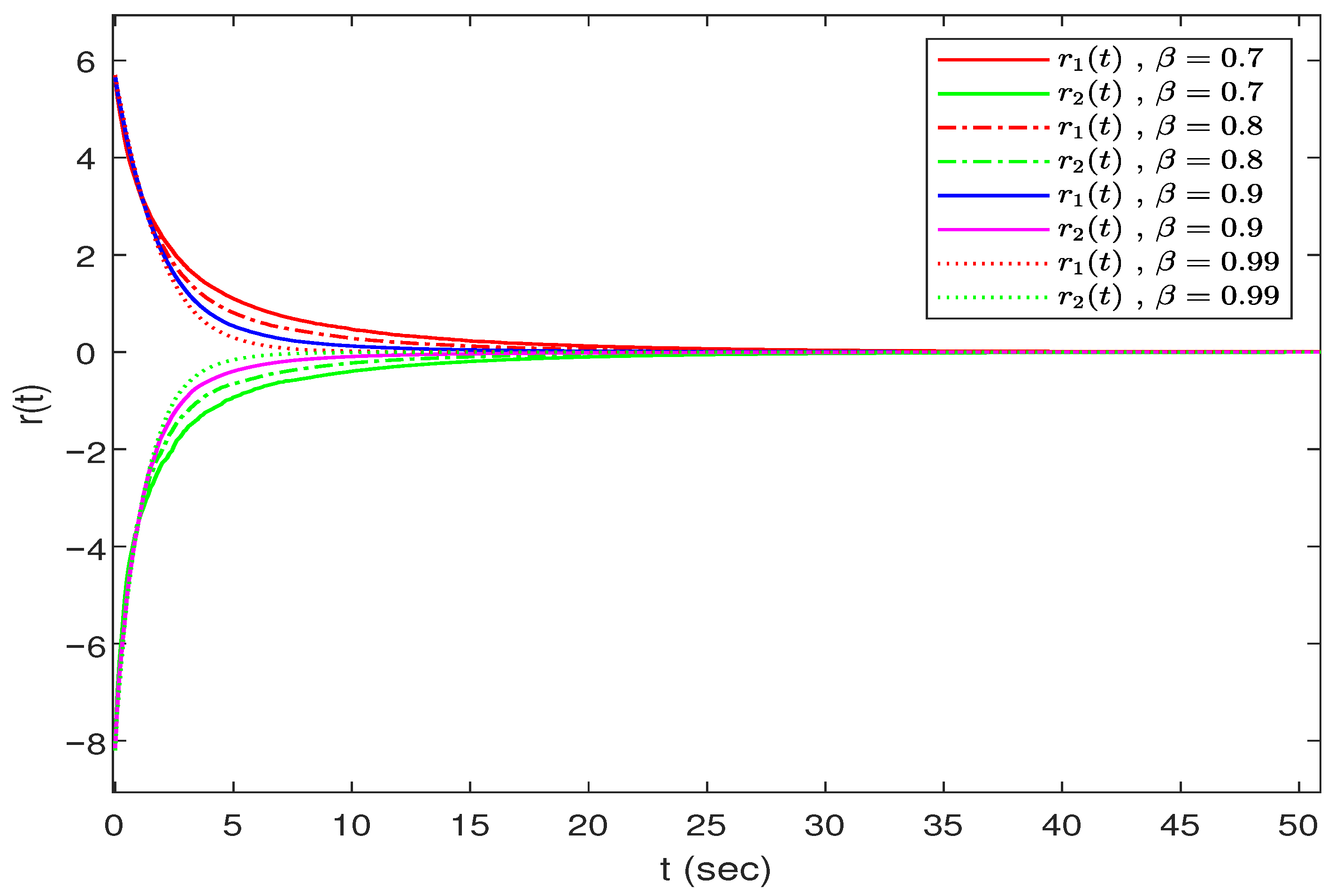
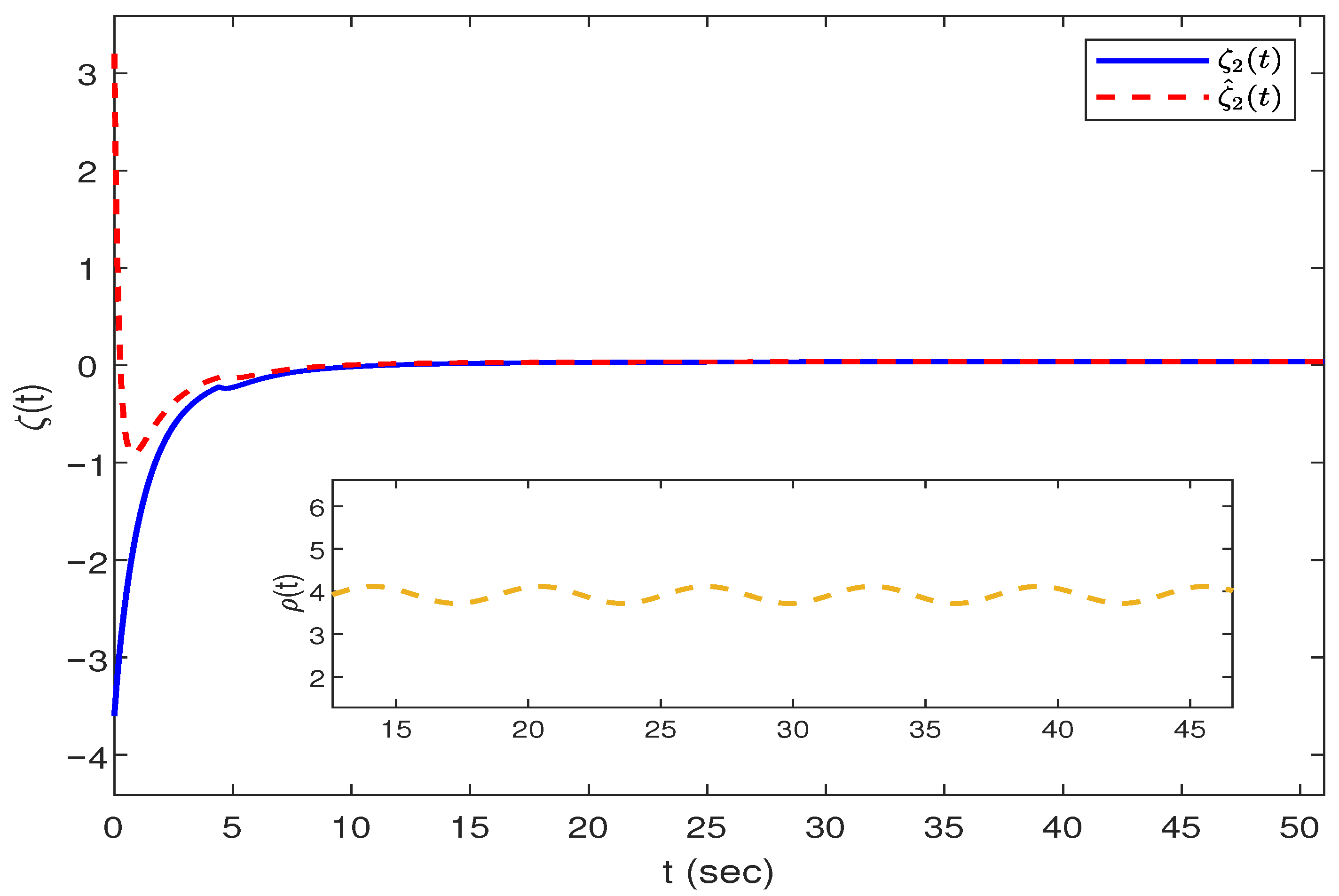
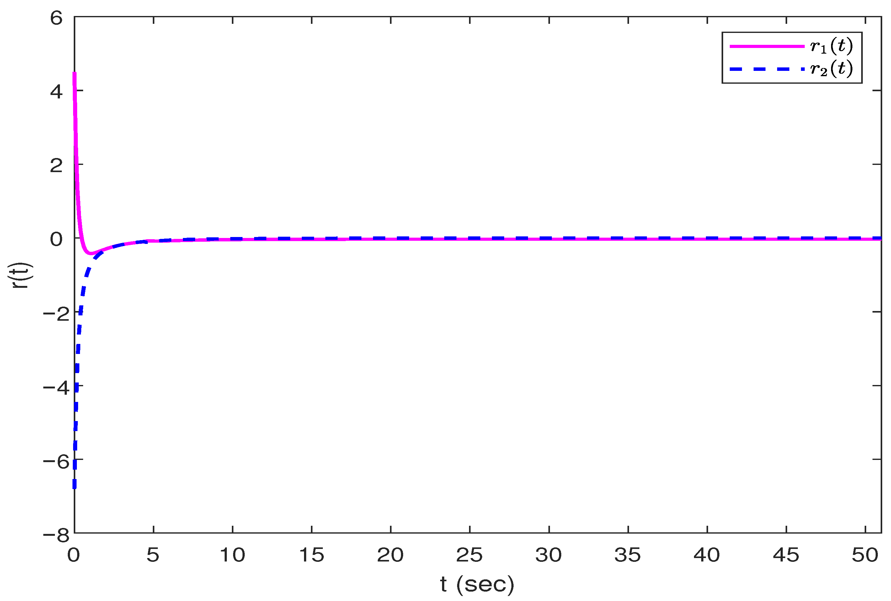
Based on the above parameters and feasible solutions, Figure 4, Figure 5 and Figure 6 show all the simulation results. Figure 4 and Figure 5 depict the trajectories of the neuronal states ${\zeta }_1\left(t\right)$ and ${\zeta }_2\left(t\right)$ and their estimated values at different orders. 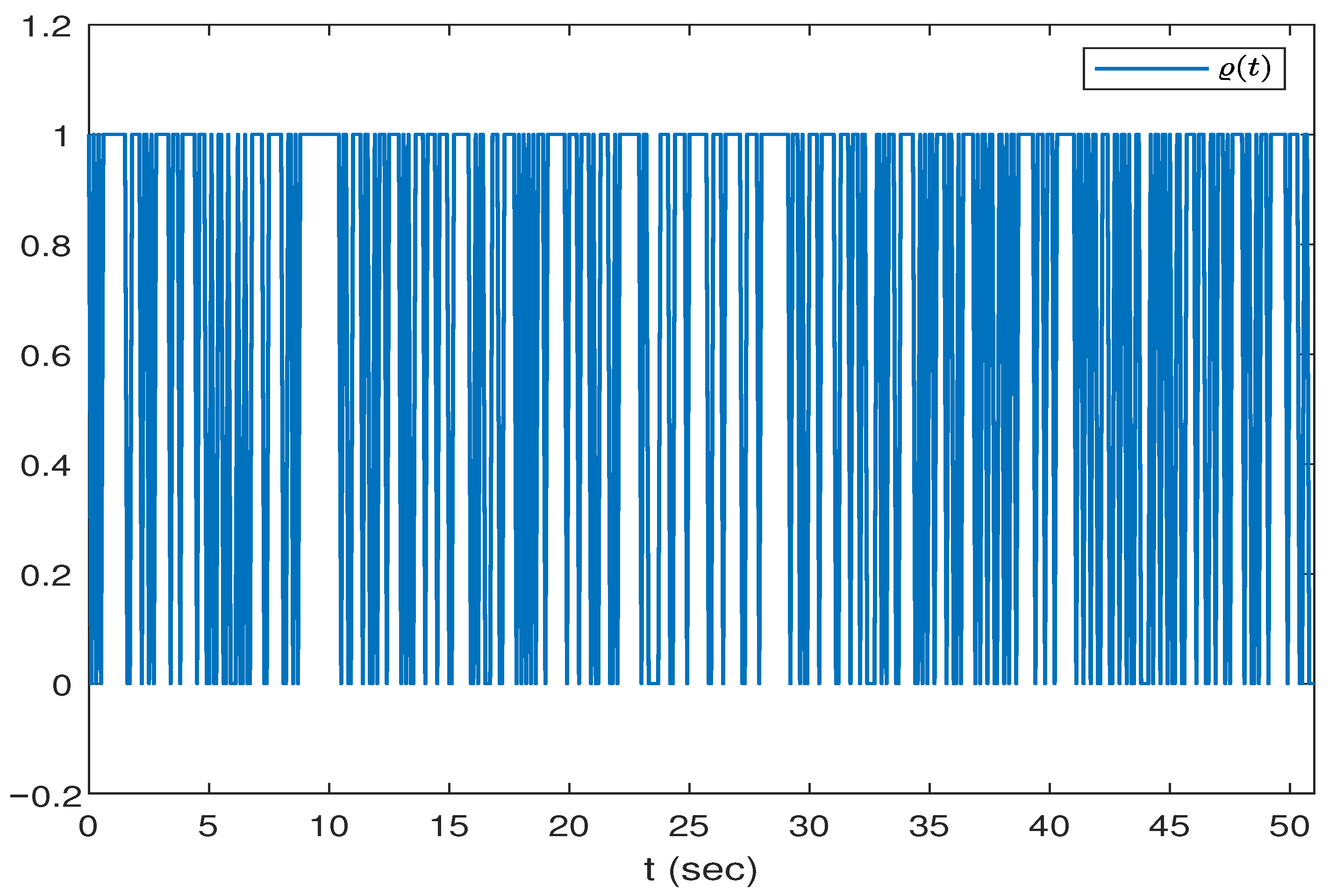Figure 6 shows the dynamic error-response curves at different orders $(\beta =\left\{0.7,0.8,0.9\right\})$, and Figure 7 indicates the value of the random variable $\varrho \left(t\right)$ when the time-varying delay $\rho \left(t\right)$ occurs randomly. 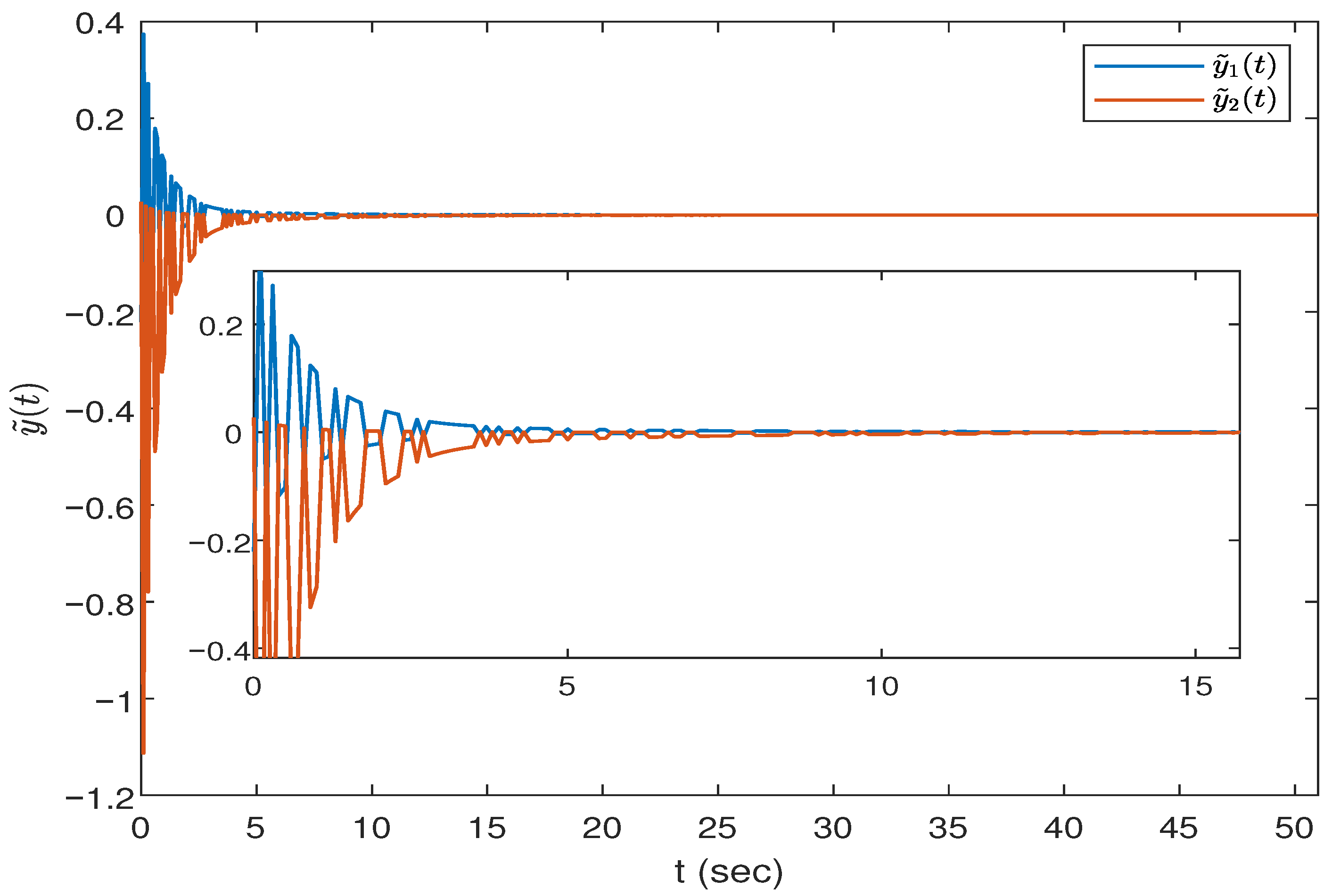Figure 8 and Figure 9 show the actual outputs of neural networks and the cyber-attacks for $y\left(t\right)$, respectively. From this, it can be seen that the fractional nonfragile state estimator designed in this paper is valid.

Example 2.

To further verify the validity and superiority of the methods provided in this example, consider the conventional FONN system [39]

$$\left\{\begin{array}{c}\begin{array}{cc}\hfill {}_{t_0}{}^{C}D_t^{\beta }\zeta \left(t\right)& =-\mathcal{C}\zeta \left(t\right)+\mathcal{A}f\left(\zeta \left(t\right)\right)+\mathcal{B}f\left(\zeta (t-\rho \left(t\right))\right)+\mathcal{E}{\int }_{t-d\left(t\right)}^{t}f\left(\zeta \left(s\right)\right)ds,\hfill \\ \hfill y\left(t\right)& =\mathcal{D}\zeta \left(t\right),\hfill \end{array}\hfill \end{array}\right.$$

(37)

with the following parameters:

$$\begin{array}{cc}\hfill \mathcal{C}& =\left[\begin{array}{cc}1& 0\\ 0& 1\end{array}\right],\mathcal{A}=\left[\begin{array}{cc}-0.8& 0.19\\ 0.5& -0.82\end{array}\right],\mathcal{B}=\left[\begin{array}{cc}-0.7& 0.8\\ 0.17& -0.6\end{array}\right],\mathcal{D}=\left[\begin{array}{cc}0.1& 0.65\\ 0& 0.15\end{array}\right].\hfill \end{array}$$

In this simulation, we choose the following activation functions:

$$\begin{array}{c}\hfill g\left(\zeta \left(t\right)\right)=\left[\begin{array}{c}-0.6{\zeta }_1\left(t\right)+tanh\left(0.3{\zeta }_1\right)+0.3{\zeta }_2\left(t\right)\\ 0.1{\zeta }_1\left(t\right)-0.2{\zeta }_2\left(t\right)+tanh\left(0.6{\zeta }_2\left(t\right)\right)\end{array}\right],\end{array}$$

which implies that

$$\begin{array}{c}\hfill {\overrightarrow{F}}_1=\left[\begin{array}{cc}-0.6& 0.3\\ 0.1& -0.2\end{array}\right],{\overrightarrow{F}}_2=\left[\begin{array}{cc}-0.3& 0.3\\ 0.1& 0.4\end{array}\right].\end{array}$$

In this example, we obtain the maximal allowable upper bounds for different $\overline{\rho }$, $\beta =0.9$, which are shown in

Table 1. Maximal allowable delays for different values $\overline{\rho }$ ($\beta =0.9$).

Methods	$\overline{\mathit{\rho }}=0.1$	$\overline{\mathit{\rho }}=0.2$	$\overline{\mathit{\rho }}=0.3$	$\overline{\mathit{\rho }}=0.5$	$\overline{\mathit{\rho }}=0.7$	$\overline{\mathit{\rho }}=0.9$
[40]	4.353	3.5514	2.4549	1.8431	1.1201	0.5829
[38]	∞	∞	∞	∞	∞	∞
Corollary 2	5.5932	4.1192	3.2484	2.1654	1.4158	0.7049

. Simultaneously, for the different $d\in \left\{0.1,0.2,0.3,0.5,0.7,0.9\right\}$, the results of MAUBs corresponding to system orders $\beta$ are presented in

Table 2. Maximal allowable delays for different orders of $\beta$ and d.

$\mathit{\beta }$	d
	0.2	0.6	1	1.4	1.8	2.2
0.6	10.416	3.5376	2.1283	1.5016	1.1452	0.9152
0.8	6.1067	2.7168	1.8559	1.4287	1.1659	0.9855
0.9	4.1192	2.5195	1.7956	1.4231	1.1878	1.0230
0.99	4.6167	2.3993	1.7634	1.4274	1.2112	1.0574

, where the system orders are selected as $\beta \in \left\{0.6,0.8,0.9,0.99\right\}$. From Table 1 and Table 2, it can be easily concluded that the methods proposed in this paper exhibit reduced conservatism.

Choose $\overline{\rho }=0.2,d=0.2$, and the allowable upper bound $\rho =4.1192$. Assume that $\rho \left(t\right)=0.2sin\left(t\right)+3.9192$ and $\zeta \left(0\right)={[2.4;-3.6]}^T,\hat{\zeta }\left(0\right)={[-2.1;3.2]}^T$. The state trajectories of the FONNs (37) are shown in Figure 10 and Figure 11. Figure 12 depicts the estimation errors. As a result, the simulation results demonstrate the effectiveness of the designed estimator (5).

5. Conclusions

This paper addresses the nonfragile SE problem for a class of memristor-based FONNs with ROTVDs and cyber-attacks. Considering the phenomenon of cyber-attacks in the network transmission process and the problem of the signal transmission burden that affects network communication in practical engineering applications, a nonfragile fractional-order state estimator, based on quantized measurement outputs, was designed. Finally, two examples were provided to verify the validity of the estimation method. In the future, we will apply the proposed method to address fractional-order linear systems with parameter uncertainties, as well as other nonlinear systems.