A Novel Fractional Order Multivariate Partial Grey Model and Its Application in Natural Gas Production

Abstract

Accurate prediction of natural gas production is of great significance for optimizing development strategies, simplifying production management, and promoting decision-making. This paper utilizes partial differentiation to effectively capture the spatiotemporal characteristics of natural gas data and the advantages of grey prediction models. By introducing the fractional damping accumulation operator, a new fractional order partial grey prediction model is established. The new model utilizes partial capture of details and features in the data, improves model accuracy through fractional order accumulation, and extends the metadata of the classic grey prediction model from time series to matrix series, effectively compensating for the phenomenon of inaccurate results caused by data fluctuations in the model. Meanwhile, the principle of data accumulation is effectively expressed in matrix form, and the least squares method is used to estimate the parameters of the model. The time response equation of the model is obtained through multiplication transformation, and the modelling steps are elaborated in detail. Finally, the new model is applied to the prediction of natural gas production in Qinghai Province, China, selecting energy production related to natural gas production, including raw coal production, oil production, and electricity generation, as relevant variables. To verify the effectiveness of the new model, we started by selecting the number of relevant variables, divided them into three categories for analysis based on the number of relevant variables, and compared them with five other grey prediction models. The results showed that in the seven simulation experiments of the three types of experiments, the average relative error of the new model was less than 2%, indicating that the new model has strong stability. When selecting the other three types of energy production as related variables, the best effect was achieved with an average relative error of 0.3821%, and the natural gas production for the next nine months was successfully predicted.

1. Introduction

Natural gas, as a clean source of fossil energy, is gradually becoming one of the main sources of energy and will be an important guarantee for China’s energy strategy and carbon emission reduction implementation for a long time [1]. Accurate forecasting of natural gas production plays an important role in optimizing development strategies, streamlining production management, and facilitating decision-making [2]. Qinghai natural gas plays an irreplaceable role in guaranteeing national energy security, promoting regional economic development, and facilitating new energy transformation. Its abundant natural gas resources and stable production and supply capacity have given Qinghai an important position in the energy map of western China. Stable production and supply are important to ensure the diversification of the national energy mix and the peaking capacity. Adequate natural gas reserves are a key factor in achieving improved energy supply capacity and new energy bases. Accurate gas production forecasts can provide strong support to governments and energy companies in developing long-term energy strategies and policies.

2. Literature Review

2.1. Introduction to Three Types of Natural Gas Production Prediction Methods

The earliest oil and gas field production prediction methods in China were life cycle models, including generalized Weng’s model and Hubbert’s model, etc., which regarded the cyclical change of production as a life cycle process and predicted it by constructing the corresponding cyclic model. For example, Chen [3] extended Weng’s prediction model by using probabilistic statistics to derive a generalized model for predicting oil and gas field production, which extended the practical value of Weng’s prediction. Chen et al. [4] proposed a model modification method based on multiplicative and exponential correction coefficients for predicting natural gas production for the traditional Weng and Weibull production prediction models. In the subsequent development, a variety of conventional decline analysis methods (e.g., Arps hyperbolic decline, Arps harmonic decline, extended exponential decline, and DUONG decline) have been widely applied to the prediction of natural gas production, and these methods have demonstrated good results in the prediction of the decline period of gas wells. For example, Chen et al. [5] conducted a detailed comparative analysis of the prediction results of four commonly used decreasing prediction models at different production stages. Despite the success of the above methods in natural gas production forecasting, there are some limitations of these models. They are prone to the phenomenon of multiple solutions, which reduces the fitting accuracy, while the model itself is not easy to generalize, and these factors may limit the effectiveness of their application to some extent.

The second category of traditional time-series forecasting methods is based on statistical principles of modelling the course, direction, and trend of a time series, which is then extended and extrapolated to achieve the forecasting objective. For example, Wang et al. [6] used the ARIMA prediction method to predict natural gas production, and the prediction results have high accuracy and are consistent with the change in coalbed methane production. Manowska et al. [7] combined an autoregressive sliding average summation model with a long and short-term memory neural network (LSTM) to construct a combined model for integrated forecasting of natural gas production. Chen et al. [8] constructed a low-cost adsorbed natural gas content estimation model based on geological parameters using a statistical learning approach, which can effectively estimate natural gas production. Smajla et al. [9] statistically analysed the natural gas consumption data and forecasted the natural gas consumption data in a short time. Kani et al. [10] developed a smooth transition regression model from a regression model and assessed and forecasted the demand for natural gas in Iran and obtained better results. All of the above statistical methods have yielded good results in natural gas production and consumption forecasting. However, general statistical learning prediction methods make it difficult to obtain parameters to meet the current needs of daily oilfield development, which affects the prediction accuracy of the model to a certain extent.

With the arrival of the big data era, oil and gas field automation technology is developing rapidly; machine learning and deep learning methods provide an effective way for the digital construction of oil and gas fields. At the same time, they have also become the current hotspot of research in various fields [11]. As a machine learning technique, artificial neural networks have shown great potential in unconventional oil and gas production. For example, Ji et al. [12] who used random forests for shale gas production prediction, solved the problem of poor accuracy of production prediction of multi-stage horizontal wells in shale gas wells under idealised models. Qiao et al. [13] constructed a combinatorial model based on wavelet transform for predicting the monthly production variance of natural gas in the United States. Zhu et al. [14] combined adaptive threshold denoising (ATD) with BP neural networks to predict shale gas well production based on reservoir modification data. In addition, Zha et al. [15] combined a neural network model (CNN) with a long short-term memory neural network (LSTM) to build a combined CNN-LSTM model to predict the monthly production of natural gas. Anđelković and Bajatović [16] used a machine learning approach to predict urban natural gas consumption from weather prediction data. These above cases of applying methods such as neural networks have yielded good results in natural gas production forecasting and can converge quickly to an acceptable solution. However, their drawbacks are that the direction of convergence may have some deviation, the stability is relatively poor, and the computational efficiency needs to be improved.

2.2. Research on Grey Prediction Model and Its Application in Natural Gas Production Prediction

The grey prediction has become a research hotspot in recent years because of its simple structure, and easy calculation, and is well-suited for small sample system research [17,18]. With the development over the past 40 years, the grey prediction model has been widely expanded from the initial GM(1,1) model through model parameter optimization [19], model structure expansion [20], and model modelling mechanism analysis [21,22,23], and has been successfully applied to a variety of domains such as transportation [24], environment [25], energy [26], and economy [27]. In natural gas production and consumption prediction, grey prediction also plays a significant role. For example, Han et al. [28] combined the grey model with the support vector machine to predict shale gas production, which provided reliable data for the later evaluation of the decreasing law of gas wells and the calculation of the recoverable reserves of gas wells. Zeng et al. [29] established a grey model with a new structure from the classical Verhulst model and applied it to national natural gas production forecasting. Ma et al. [30] combined the kernel ridges of generalized Morlet wavelets with the depth of a grey prediction model to establish a combined model and applied it to natural gas production forecasting. Ding [31] established a new adaptive intelligent grey model and applied it to natural gas demand forecasting in China. Hu et al. [32] established a new multi-order time-lagged fractional grey model using the fractional order principle for the phenomenon of time-lagged natural gas consumption in the Chinese manufacturing industry. These are the development processes of the grey forecasting model and its application to natural gas production, demand, and consumption, which have achieved better results.

2.3. Research Limitations, Contributions, and Structure of This Paper

However, both univariate and multivariate grey models use time series as inputs. The metadata used in the literature [28,29,30,31,32] for applications in natural gas systems is time series in the form of vectors, which is processed in such a way that the spatio-temporal characteristics of the data are relatively weakly represented. To more fully represent the spatio-temporal properties of the data, the input data can be expanded from vector form to matrix form. Duan and Wang [33] established a partial differential grey prediction model for the spatio-temporal nature of traffic flow, which was successfully applied to short-time traffic flow prediction. Zhou and Duan [11] used the volatility of traffic flow data to establish a grey prediction model with second-order partial differentiation from the nature of traffic flow and applied it to short-time traffic flow.

At the same time, the grey multivariate model mentioned above for natural gas production forecasting takes into account relevant variables that are factors other than energy production. Aiming at the spatio-temporal characteristics of natural gas production data and combining the advantages of high prediction accuracy of the grey GMC(1,N) model, this paper establishes a new partial grey prediction model. To verify the validity of the new model, the monthly data of natural gas production in Qinghai, China, as well as related serial data of oil, raw coal production, and electricity production are used as inputs. The results show that the new model exhibits good stability and its prediction is much better than the other five grey prediction models. The contributions of this paper are as follows:

• Given the spatiotemporal and nonlinear characteristics of natural gas production data, this paper utilizes the advantages of partial differentiation to effectively capture details and features in the data. Fractional order damping accumulation can improve model accuracy and effectively compensate for the phenomenon of inaccurate results caused by data fluctuations. A new fractional order multivariate biased grey prediction model is established.
• In terms of model structure, the classic grey prediction model is extended from ordinary differential form to partial differential form, and the fractional order accumulation principle is integrated into the partial grey prediction model to expand the structure of the classic grey prediction model. This improvement enables the model to more effectively capture various complex features such as time and space of data, improve model accuracy, and greatly broaden the structural framework and scope of application of the grey prediction model.
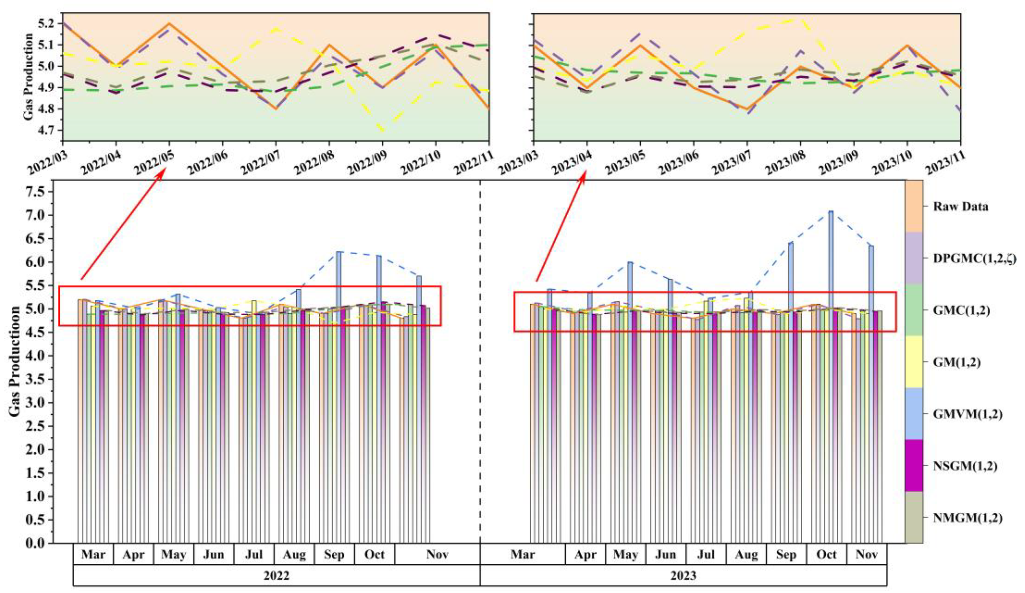
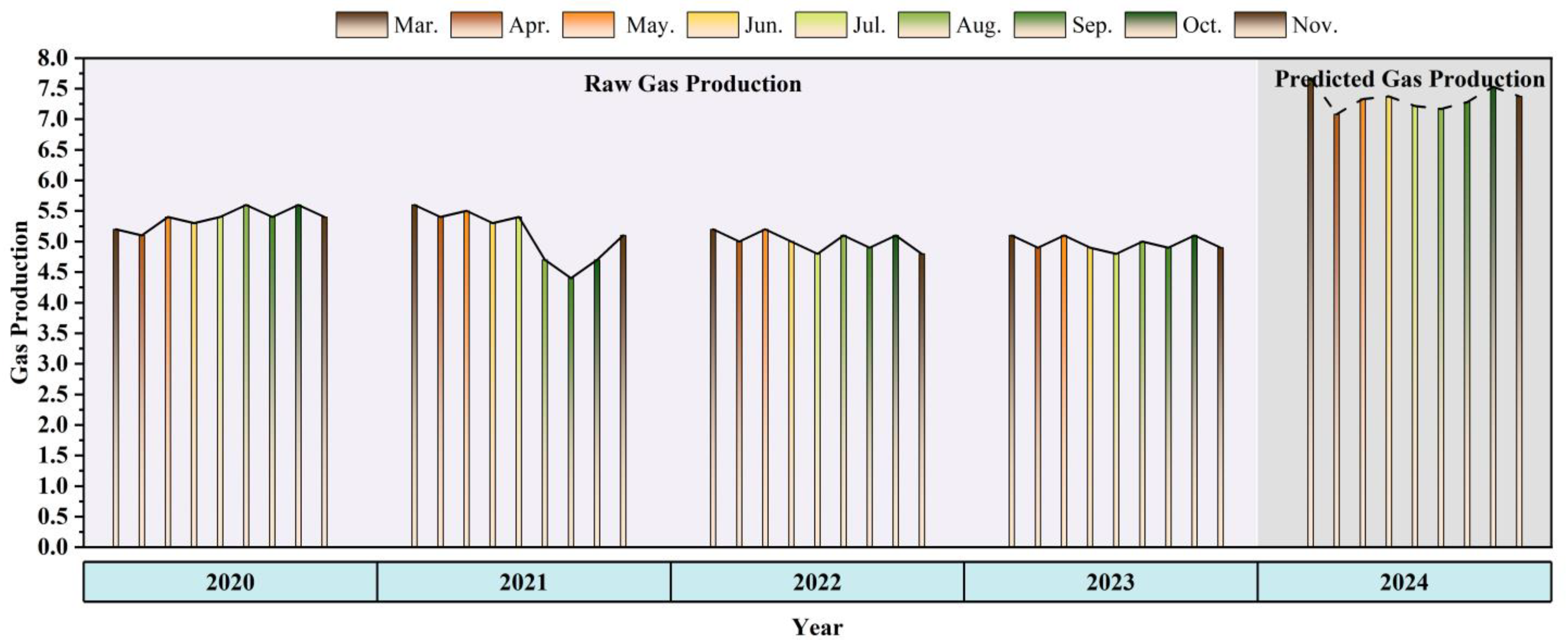
• In terms of application practice, this study applies the newly constructed partial grey prediction to the field of natural gas production forecasting. Based on the selection of oil, raw coal, and electricity production as the relevant series, the validity of the model is analysed in-depth through seven specific cases in three categories. The results showed that the average relative error of the new model was around 1% in all seven cases, and its prediction performance is significantly better than the other five grey prediction models. In addition, the model has successfully achieved an accurate forecast of natural gas production for the next nine months.

The rest of the paper is organized as follows: Section 3 develops a fractional order multivariate partial grey model and examines the parameter estimation and modelling steps of the model. Section 4 analyses the validity of the new model using data on natural gas and three types of energy production in Qinghai, China. Section 5 applies the new model to the problem of forecasting monthly natural gas production and analyses the results. Finally, Section 6 gives the conclusions of the study and proposes relevant policies.

In the full text, the different abbreviations are for different grey prediction models. Abbreviations and their meanings are listed in

Table 1. Abbreviations of the models.

Number	Abbreviation	Definition
1	GM(1,1)	Grey model with one variable and one first order equation
2	GMC(1,N)	A first-order n-variable grey differential equation model [34]
3	GM(1,N)	Grey model of the first order with n variables [35]
4	GMVM(1,N)	The grey multivariable Verhulst model [36]
5	NSGM(1,N)	The new structured grey model [37]
6	NMGM(1,N)	Novel multi-variable grey model [38]
7	DPGMC(1,N,ζ)	The damping fractional order multivariate partial grey prediction model

.

3. Modelling Partial Grey Differential Equations in First-Order Individual Variables

3.1. Grey Differential Equation Model with First-Order Individual Variables

This section introduces the damping accumulation generation operator into the partial grey prediction model, establishes a new fractional order partial grey prediction model, estimates the model process parameters, optimizes the fractional order using the particle swarm optimization algorithm, solves the time response equation of the model, and obtains the modelling steps.

Definition 1. 

Let  $X_1^{(0)}=(x_1^{(0)}(1),x_1^{(0)}(2),\dots ,x_1^{(0)}(n))$ be a sequence of system characteristic data, $X_r^{(0)}=(x_r^{(0)}(1),$ $x_r^{(0)}(2),\dots ,x_r^{(0)}(n)),r=2,3,\dots ,N$ is the sequence of relevant factors. $X_r^{(1)}$ is the accumulative generation sequence (1-AGO) of the original sequence $X_r^{(0)}$, $r=1,2,\dots ,N$, $Z_1^{(1)}$ is the mean sequence generated by consecutive neighbours of $X_1^{(1)}$, establishing the whitening equation:

$${\displaystyle \frac{d{X}_1^{(1)}(t)}{dt}}+a{X}_1^{(1)}(t)=b_2{X}_2^{(1)}(t)+b_3{X}_3^{(1)}(t)+\dots +b_N{X}_N^{(1)}(t)+u$$

(1)

is a first-order n-variable grey differential equation model, denoted GMC(1,N). Where  $a$  is called the system development coefficient,  $u$  is the grey control parameter of the system,  $b_r(r=2,3,\dots ,N)$  is the driving coefficient, and  $b_r{X}_r^{(1)}(t)(r=2,3,\dots ,N)$  is the driving term.

Let

$$f(t)=b_2{X}_2^{(1)}(t)+b_3{X}_3^{(1)}(t)+\dots +b_N{X}_N^{(1)}(t)+u$$

(2)

The model solution for the system 1-AGO sequence can be obtained as

$${\widehat{X}}_1^{(1)}(t)=X_1^{(1)}(1)e^{-b_1(t-1)}+{\displaystyle {\int }_1^t{e}^{-b_1(t-\tau )}f(\tau )d\tau }$$

(3)

The convolution integral term ${\displaystyle {\int }_1^t{e}^{-b_1(t-\tau )}f(\tau )d\tau }$ in Equation (7) can be approximated by the convolution method and the trapezoidal norm in the discrete domain, and the following model solution is obtained from the initial value ${\widehat{X}}_1^{(1)}(1)=X_1^{(1)}(1)=X_1^{(0)}(1)$. This leads to the following theorem.

Theorem 1. 

Solution of the GMC(1,N) model

$${\widehat{X}}_1^{(1)}(t)\cong X_1^{(0)}(1)e^{-b_1(t-1)}+{\displaystyle \frac{1}{2}}{e}^{-b_1(t-1)}f(1)+{\displaystyle \frac{1}{2}}f(t)+{\displaystyle \sum _{\tau =2}^{t-1}[e^{-b_1(t-\tau )}f(\tau )]}$$

(4)

Doing a cumulative generative operation on  ${\widehat{X}}_1^{(1)}(t)$  gives the  ${\widehat{X}}_1^{(0)}(t)$  whitened value, which is the predicted value.

$$\left\{\begin{array}{l}{\widehat{X}}_1^{(0)}(1)={\widehat{X}}_1^{(1)}(1)\hfill \\ {\widehat{X}}_1^{(0)}(t)={\widehat{X}}_1^{(1)}(t)-{\widehat{X}}_1^{(1)}(t-1),t=2,3,\dots ,n\hfill \end{array}\right.$$

(5)

3.2. Modelling Partial Grey Differential Equations in First-Order Individual Variables

Definition 2. 

Assuming there is a non-negative equidistant sequence $X^{(0)}=\left\{x^{(0)}(1),x^{(0)}(2),\dots ,x^{(0)}(n)\right\}\left(x^{(0)}(k)>0\right)$, $X^{(\xi )}=\left\{x^{(\xi )}(1),x^{(\xi )}(2),\dots ,x^{(\xi )}(n)\right\}$ is an $\xi$ order damping accumulation sequence of $X^{(0)}$.

The damping accumulation generation operator  $\left(\xi -AGO\right)$  is defined as

$$x^{(\xi )}(k)={\displaystyle \sum _{i=1}^k\left(\frac{x^{(0)}(i)}{{\xi }^{i-1}}\right),k=1,2,\dots ,n,\xi \in (0,1]}$$

(6)

The matrix representation of  $\xi$  order damping accumulation is

$$\left[\begin{array}{c}{x}^{(\xi )}(1)\\ x^{(\xi )}(2)\\ x^{(\xi )}(3)\\ ⋮\\ x^{(\xi )}(n)\end{array}\right]=\left[\begin{array}{ccccc}1& 0& 0& \dots & 0\\ 1& {\displaystyle \frac{1}{\xi }}& 0& \dots & 0\\ 1& {\displaystyle \frac{1}{\xi }}& {\displaystyle \frac{1}{{\xi }^2}}& \dots & 0\\ ⋮& ⋮& ⋮& \ddots & ⋮\\ 1& {\displaystyle \frac{1}{\xi }}& {\displaystyle \frac{1}{{\xi }^2}}& \dots & {\displaystyle \frac{1}{{\xi }^{n-1}}}\end{array}\right]\left[\begin{array}{c}{x}^{(0)}(1)\\ x^{(0)}(2)\\ x^{(0)}(3)\\ ⋮\\ x^{(0)}(n)\end{array}\right]$$

(7)

Firstly, the definition of matrix sequence is given as follows

Definition 3. 

Let  $X_r^{(0)}(r=1,2,\dots ,N)$ be a matrix sequence formed by $n$ $m\times m$ order matrices

$$\begin{array}{l}{X}_1^{(0)}=(X_1^{(0)}(1),X_1^{(0)}(2),\dots ,X_1^{(0)}(n))\\ X_2^{(0)}=(X_2^{(0)}(1),X_2^{(0)}(2),\dots ,X_2^{(0)}(n))\\ ⋮\\ X_N^{(0)}=(X_N^{(0)}(1),X_N^{(0)}(2),\dots ,X_N^{(0)}(n))\end{array}$$

(8)

where

$$X_r^{(0)}(k)=\left[\begin{array}{cccc}{X}_{r(1,1)}^{(0)}(k)& X_{r(1,2)}^{(0)}(k)& \dots & X_{r(1,m)}^{(0)}(k)\\ X_{r(2,1)}^{(0)}(k)& X_{r(2,2)}^{(0)}(k)& \dots & X_{r(2,m)}^{(0)}(k)\\ ⋮& ⋮& \ddots & ⋮\\ X_{r(m,1)}^{(0)}(k)& X_{r(m,2)}^{(0)}(k)& \dots & X_{r(m,m)}^{(0)}(k)\end{array}\right],(r=1,2,\dots ,N,k=1,2,\dots ,n)$$

where $X_{r(i,j)}^{(0)}(k)$ represents the values of $X_r^{(0)}(k)$ in rows $i$ and columns $j$.

Definition 4. 

$X_r^{(\xi )}(r=1,2,\dots ,N)$ is the damping accumulation generated sequence of the original matrix sequence  $X_r^{(0)}(r=1,2,\dots ,N)$

$$\begin{array}{l}{X}_1^{(\xi )}=(X_1^{(\xi )}(1),X_1^{(\xi )}(2),\dots ,X_1^{(\xi )}(n))\\ X_2^{(\xi )}=(X_2^{(\xi )}(1),X_2^{(\xi )}(2),\dots ,X_2^{(\xi )}(n))\\ ⋮\\ X_N^{(\xi )}=(X_N^{(\xi )}(1),X_N^{(\xi )}(2),\dots ,X_N^{(\xi )}(n))\end{array}$$

(9)

where

$$X_r^{(\xi )}(k)=\left[\begin{array}{cccc}{X}_{r(1,1)}^{(\xi )}(k)& X_{r(1,2)}^{(\xi )}(k)& \dots & X_{r(1,m)}^{(\xi )}(k)\\ X_{r(2,1)}^{(\xi )}(k)& X_{r(2,2)}^{(\xi )}(k)& \dots & X_{r(2,m)}^{(\xi )}(k)\\ ⋮& ⋮& \ddots & ⋮\\ X_{r(m,1)}^{(\xi )}(k)& X_{r(m,2)}^{(\xi )}(k)& \dots & X_{r(m,m)}^{(\xi )}(k)\end{array}\right],(r=1,2,\dots ,N,k=1,2,\dots ,n)$$

$X^{(\xi )}(k)={\displaystyle \sum _{i=1}^k\left(\frac{X^{(0)}(i)}{{\xi }^{i-1}}\right)=\left[\begin{array}{cccc}1& 0& \dots & 0\\ 1& \frac{1}{\xi }& \dots & 0\\ ⋮& ⋮& \ddots & ⋮\\ 1& \frac{1}{\xi }& \dots & \frac{1}{{\xi }^{k-1}}\end{array}\right]X^{(0)}(k),\xi \in (0,1]}$, $X_{r(i,j)}^{(\xi )}(k)$ represents the values of $X_r^{(\xi )}(k)$ in rows $i$ and columns $j$.

Definition 5. 

$Z_1^{(1)}$ is the mean sequence generated by consecutive neighbours of  $X_1^{(1)}$

$$Z_1^{(\xi )}=(Z_1^{(\xi )}(1),Z_1^{(\xi )}(2),\dots ,Z_1^{(\xi )}(n))$$

(10)

where

$$Z_1^{(\xi )}(k)=\left[\begin{array}{cccc}{Z}_{1(1,1)}^{(\xi )}(k)& Z_{1(1,2)}^{(\xi )}(k)& \dots & Z_{1(1,m)}^{(\xi )}(k)\\ Z_{1(2,1)}^{(\xi )}(k)& Z_{1(2,2)}^{(\xi )}(k)& \dots & Z_{1(2,m)}^{(\xi )}(k)\\ ⋮& ⋮& \ddots & ⋮\\ Z_{1(m,1)}^{(\xi )}(k)& Z_{1(m,2)}^{(\xi )}(k)& \dots & Z_{1(m,m)}^{(\xi )}(k)\end{array}\right],(k=1,2,\dots ,n)$$

$Z_r^{(\xi )}(k)={\displaystyle \frac{X_r^{(\xi )}(k-1)+X_r^{(\xi )}(k)}{2}},(k=2,\dots ,n)$. $Z_{1(i,j)}^{(\xi )}(k)$ represents the values of $Z_1^{(\xi )}(k)$ in rows $i$ and columns $j$.

Definition 6. 

$Z_{1x}^{(\xi )}$ and  $Z_{1y}^{(\xi )}$  represent the horizontal and vertical partial derivative matrix sequence of  $Z_1^{(\xi )}$, respectively,

$$Z_{1x}^{(\xi )}(k)=\left[\begin{array}{cccc}{Z}_{1x(1,1)}^{(\xi )}(k)& Z_{1x(1,2)}^{(\xi )}(k)& \dots & Z_{1x(1,m)}^{(\xi )}(k)\\ Z_{1x(2,1)}^{(\xi )}(k)& Z_{1x(2,2)}^{(\xi )}(k)& \dots & Z_{1x(2,m)}^{(\xi )}(k)\\ ⋮& ⋮& \ddots & ⋮\\ Z_{1x(m,1)}^{(\xi )}(k)& Z_{1x(m,2)}^{(\xi )}(k)& \dots & Z_{1x(m,m)}^{(\xi )}(k)\end{array}\right],(k=2,3,\dots ,n)$$

$$Z_{1y}^{(\xi )}(k)=\left[\begin{array}{cccc}{Z}_{1y(1,1)}^{(\xi )}(k)& Z_{1y(1,2)}^{(\xi )}(k)& \dots & Z_{1y(1,m)}^{(\xi )}(k)\\ Z_{1y(2,1)}^{(\xi )}(k)& Z_{1y(2,2)}^{(\xi )}(k)& \dots & Z_{1y(2,m)}^{(\xi )}(k)\\ ⋮& ⋮& \ddots & ⋮\\ Z_{1y(m,1)}^{(\xi )}(k)& Z_{1y(m,2)}^{(\xi )}(k)& \dots & Z_{1y(m,m)}^{(\xi )}(k)\end{array}\right],(k=2,3,\dots ,n)$$

$Z_{1x(i,j)}^{(\xi )}(k)$ represents the values of $Z_{1x}^{(\xi )}(k)$ in rows $i$ and columns $j$. $Z_{1x(i,j)}^{(\xi )}$, $Z_{1y(i,j)}^{(\xi )}$ satisfy the following property:

Property 1. 

Let $Z_{1x(i,j)}^{(\xi )}$,  $Z_{1y(i,j)}^{(\xi )}$  be the values of  $Z_{1x}^{(\xi )}$,  $Z_{1y}^{(\xi )}$  respectively, in rows  $i$  and columns  $j$  and satisfy the following two conditions:

(1)

$Z_{1x(i,j)}^{(\xi )}(k)=Z_{1(i,j)}^{(\xi )}(k)-Z_{1(i-1,j)}^{(\xi )}(k)$

(2)

$Z_{1y(i,j)}^{(\xi )}(k)=Z_{1(i,j)}^{(\xi )}(k)-Z_{1(i,j-1)}^{(\xi )}(k)$

Definition 7. 

Let $X_1^{(0)}(k)$, $X_r^{(\xi )}(k)$, $Z_1^{(\xi )}(k)$, $Z_{1x}^{(\xi )}(k)$, $Z_{1y}^{(\xi )}(k)$ as defined in 3–6, the grey derivatives ${\displaystyle \frac{d{x}_1^{(\xi )}(k)}{dk}}=X_1^{(\xi )}(k)-X_1^{(\xi )}(k-1)$, $Z_r^{(\xi )}(k)$ is the background value of the sequence, which can be obtained using the trapezoidal formula $Z_r^{(\xi )}(k)={\displaystyle \frac{X_r^{(\xi )}(k-1)+X_r^{(\xi )}(k)}{2}}$,

$$X_1^{(\xi )}(k)-X_1^{(\xi )}(k-1)+a{Z}_{1x}^{(\xi )}(k)+b{Z}_{1y}^{(\xi )}(k)+c{Z}_1^{(\xi )}(k)={\displaystyle \sum _{r=2}^N{b}_r{X}_r^{(\xi )}(k)+\mu }$$

(11)

is the damping fractional order multivariate partial grey prediction model, abbreviated as DPGMC(1,N,ζ), where,  $a,b,c,b_2,\dots b_N$  are the parameter estimation variable, and  $\mu$  is the  $m\times m$  constant matrix:

$$\mu =\left[\begin{array}{cccc}{\mu }_{11}& {\mu }_{12}& \dots & {\mu }_{1m}\\ {\mu }_{21}& {\mu }_{22}& \dots & {\mu }_{2m}\\ ⋮& ⋮& \ddots & ⋮\\ {\mu }_{m1}& {\mu }_{m1}& \dots & {\mu }_{mm}\end{array}\right]$$

$${\displaystyle \frac{d{X}_1^{(\xi )}(t)}{dt}}+a{\displaystyle \frac{\partial X_1^{(\xi )}(t)}{\partial x}}+b{\displaystyle \frac{\partial X_1^{(\xi )}(t)}{\partial y}}+c{X}_1^{(\xi )}(t)=b_2{X}_2^{(\xi )}(t)+b_3{X}_3^{(\xi )}(t)+\dots +b_N{X}_N^{(\xi )}(t)+u$$

(12)

is the whitening equation of DPGMC (1,N,ζ).

Theorem 2. 

Least squares calculation of parameter vectors for the DPGMC(1,N,ζ)

$$\widehat{p}={[a,b,c,b_2,\dots b_N,{\mu }_{11},\dots {\mu }_{mm}]}^T$$

satisfies

$$\widehat{p}={(B^{T}B)}^{-1}{B}^{T}Y$$

(13)

where

$$B=\left[\begin{array}{cccccccccc}-Z_{1x(1,1)}^{(\xi )}(2)& -Z_{1y(1,1)}^{(\xi )}(2)& -Z_{1(1,1)}^{(\xi )}(2)& X_{2(1,1)}^{(\xi )}(2)& \dots & X_{N(1,1)}^{(\xi )}(2)& 1& 0& \dots & 0\\ -Z_{1x(1,2)}^{(\xi )}(2)& -Z_{1y(1,2)}^{(\xi )}(2)& -Z_{1(1,2)}^{(\xi )}(2)& X_{2(1,2)}^{(\xi )}(2)& \dots & X_{N(1,2)}^{(\xi )}(2)& 0& 1& \dots & 0\\ ⋮& ⋮& ⋮& ⋮& & ⋮& ⋮& & & ⋮\\ -Z_{1x(i,j)}^{(\xi )}(k)& -Z_{1y(i,j)}^{(\xi )}(k)& -Z_{1(i,j)}^{(\xi )}(k)& X_{2(i,j)}^{(\xi )}(\mathrm{k})& \dots & X_{N(i,j)}^{(\xi )}(k)& 0& 0& \dots & 0\\ ⋮& ⋮& ⋮& ⋮& & ⋮& ⋮& & & ⋮\\ -Z_{1x(m,m)}^{(\xi )}(n)& -Z_{1y(m,m)}^{(\xi )}(n)& -Z_{1(m,m)}^{(\xi )}(n)& X_{2(m,m)}^{(\xi )}(n)& \dots & X_{N(m,m)}^{(\xi )}(n)& 0& 0& \dots & 1\end{array}\right]$$

$$Y=\left[\begin{array}{c}{X}_{1(1,1)}^{(\xi )}(2)-X_{1(1,1)}^{(\xi )}(1)\\ X_{1(1,2)}^{(\xi )}(2)-X_{1(1,2)}^{(\xi )}(1)\\ ⋮\\ X_{1(i,j)}^{(\xi )}(k)-X_{1(i,j)}^{(\xi )}(k-1)\\ ⋮\\ X_{1(m,m)}^{(\xi )}(n)-X_{1(m,m)}^{(\xi )}(n-1)\end{array}\right]$$

Proof. 

Referring to the proof process of Theorem 1 in the literature [11]. □

Theorem 3. 

The time response sequence of the DPGMC(1,N,ζ) is as follows:

$${\widehat{X}}_1^{(\xi )}(k)={\displaystyle \frac{{\displaystyle \sum _{r=2}^N{b}_r{X}_r^{(\xi )}(k)+\mu }-a{Z}_{1x}^{(\xi )}(k)-b{Z}_{1y}^{(\xi )}(k)-\left(\frac{1}{2}c-1\right)X_1^{(\xi )}(k-1)}{\frac{1}{2}c+1}}$$

Perform the inverse operation of $\xi -AGO$, the cumulative reduction value can be obtained as

$${\widehat{X}}_1^{(0)}(k)=\left\{\begin{array}{cc}{X}_1^{(0)}(1)& k=1\\ \left({\widehat{X}}_1^{(\xi )}(k)-{\widehat{X}}_1^{(\xi )}(k-1)\right){\xi }^{k-1}& k=2,3,\dots \end{array}\right.$$

(14)

Proof. 

Carrying $Z_r^{(\xi )}(k)={\displaystyle \frac{X_r^{(\xi )}(k-1)+X_r^{(\xi )}(k)}{2}}$  into Equation (11) gives 

$$X_1^{(\xi )}(k)-X_1^{(\xi )}(k-1)+a{Z}_{1x}^{(\xi )}(k)+b{Z}_{1y}^{(\xi )}(k)+c{\displaystyle \frac{X_r^{(\xi )}(k-1)+X_r^{(\xi )}(k)}{2}}={\displaystyle \sum _{r=2}^N{b}_r{X}_r^{(\xi )}(k)+\mu }$$

then 

$$\left(1+{\displaystyle \frac{1}{2}}c\right)X_1^{(\xi )}(k)={\displaystyle \sum _{r=2}^N{b}_r{X}_r^{(\xi )}(k)+\mu }-\left({\displaystyle \frac{1}{2}}c-1\right)X_1^{(\xi )}(k-1)-a{Z}_{1x}^{(\xi )}(k)-b{Z}_{1y}^{(\xi )}(k)$$

so

$${\widehat{X}}_1^{(\xi )}(k)={\displaystyle \frac{{\displaystyle \sum _{r=2}^N{b}_r{X}_r^{(\xi )}(k)+\mu }-a{Z}_{1x}^{(\xi )}(k)-b{Z}_{1y}^{(\xi )}(k)-\left(\frac{1}{2}c-1\right)X_1^{(\xi )}(k-1)}{\frac{1}{2}c+1}}$$

Therefore, the reduction is reduced to

$${\widehat{X}}_1^{(0)}(k)=\left\{\begin{array}{cc}{X}_1^{(0)}(1)& k=1\\ \left({\widehat{X}}_1^{(\xi )}(k)-{\widehat{X}}_1^{(\xi )}(k-1)\right){\xi }^{k-1}& k=2,3,\dots \end{array}\right.$$

Theorem 3 is proven. □

Due to the DPGMC (1,N,ζ) using accumulation before restoration, the accumulation sequence helps smooth the data and reduce fluctuations. In the parameter-solving stage, the objective function is usually to minimise the fitting error of the cumulative sequence. However, the goal of modelling is to minimise the fitting error of the raw data. Therefore, the errors introduced during the restoration process cannot be ignored. The following theorem can explain the relationship between the accuracy of model prediction and the cumulative order ζ.

Theorem 4. 

$X_1^{(\xi )}=\left\{X_1^{(\xi )}(1),X_1^{(\xi )}(2),\dots ,X_1^{(\xi )}(k)\right\}$ is the damping accumulation generated sequence for the main $X_1^{(0)}$ column, and ${\widehat{X}}_1^{(0)}=\left\{{\widehat{X}}_1^{(0)}(1),{\widehat{X}}_1^{(0)}(2),\dots ,{\widehat{X}}_1^{(0)}(k)\right\}$ is the fitted restoration value for the main $X_1^{(0)}$ sequence. If $\left|X_1^{(\xi )}(k)-{\widehat{X}}_1^{(\xi )}(k)\right|<\epsilon$, $(k=1,2,\dots ,n)$, then $\left|X_1^{(0)}(k)-{\widehat{X}}_1^{(0)}(k)\right|<2\epsilon {\xi }^{k-1}$.

Proof. 

Because $X_1^{(\xi )}(1)=X_1^{(0)}(1)$, $\left|X_1^{(\xi )}(1)-X_1^{(0)}(1)\right|<\epsilon$, $\forall k\in \left\{1,2,\dots ,n\right\}$, $\left|X_1^{(\xi )}(k)-{\widehat{X}}_1^{(\xi )}(k)\right|<\epsilon$,

Then

$$\begin{array}{cc}\hfill \left|X_1^{(0)}(k)-{\widehat{X}}_1^{(0)}(k)\right|& =\left|\left(X_1^{(\xi )}(k)-X_1^{(\xi )}(k-1)\right){\xi }^{k-1}-\left({\widehat{X}}_1^{(\xi )}(k)-{\widehat{X}}_1^{(\xi )}(k-1)\right){\xi }^{k-1}\right|\hfill \\ & =\left|\left(X_1^{(\xi )}(k)-X_1^{(\xi )}(k-1)-{\widehat{X}}_1^{(\xi )}(k)+{\widehat{X}}_1^{(\xi )}(k-1)\right){\xi }^{k-1}\right|\hfill \\ & \le \left(\left|X_1^{(\xi )}(k)-{\widehat{X}}_1^{(\xi )}(k)\right|+\left|X_1^{(\xi )}(k-1)-{\widehat{X}}_1^{(\xi )}(k-1)\right|\right)\left|{\xi }^{k-1}\right|\hfill \\ & \le 2\epsilon {\xi }^{k-1}.\hfill \end{array}$$

Theorem 4 is proven. □

When ζ is small, especially $\xi <1$, the restoration error is $2\epsilon {\xi }^{k-1}<\epsilon$. Therefore, to reduce the restoration error, the range of ζ is set to [0, 1].

The damping accumulation generation operator in the DPGMC(1,N,ζ) model sets different weights to distinguish the influence of new and old data on the predicted values. The data after damping accumulation is more in line with the trend of exponential growth, ensuring the calculation accuracy of the DPGMC(1,N,ζ) model. This ensured the computational accuracy of the DPGMC(1,N,ζ) model.

3.3. Modelling Steps and Modelling Process for the DPGMC(1,N,ζ)

From the sequence definition in Section 2.2, the definition and parameter estimation of the DPGMC(1,N,ζ) model, and the time response equation, the main modelling steps of the model are given as follows:

Step 1. Input raw data. By Definition 3, input the matrix sequence of raw data, where $X_1^{(0)}$ is the main sequence, $X_2^{(0)},X_3^{(0)},\dots ,X_N^{(0)}$ are the correlation sequence.

Step 2. Processing the matrix sequence. Definition 2 calculates the damping accumulation to generate the matrix sequence $X_i^{(\xi )}(i=1,2,\dots ,N)$, Definition 5 calculates the adjacent mean of $X_1^{(0)}$ to generate the matrix sequence $Z_1^{(\xi )}$, and Definition 6 calculates the horizontal and vertical partial derivative matrix sequences $Z_{1x}^{(\xi )}$ and $Z_{1y}^{(\xi )}$ of $Z_1^{(\xi )}$.

Step 3. Estimate the parameters and build the model. Use Theorem 2 to construct the matrix $B,Y$ and compute the values of the parameter estimation vectors $\widehat{p}={(B^{T}B)}^{-1}{B}^{T}Y$, using the particle swarm optimization algorithm to perform optimisation calculation on ζ.

Step 4. Calculate the simulated values. Calculate the simulated value ${\widehat{X}}_1^{(0)}$ using equation Theorem 3.

Step 5. Calculation error. Mean Absolute Percentage Error (MAPE), Mean Absolute Error (MAE), Mean Square Error (MSE), R-squared ($R^2$), and Root Mean Squared Error (RMSE), are used to test prediction performance. ${\overline{X}}_1^{(0)}(k)$ is the average value of the real data. Their definitions are as follows:

$$MAPE={\displaystyle \frac{1}{n}}({\displaystyle \sum _{k=1}^m\frac{|X_1^{(0)}(k)-{\widehat{X}}_1^{(0)}(k)|}{X_1^{(0)}(k)}})\times 100\%,k=1,2,\dots ,n$$

(15)

$$MAE={\displaystyle \frac{1}{n}}{\displaystyle \sum _{k=1}^n\left|X_1^{(0)}(k)-{\widehat{X}}_1^{(0)}(k)\right|},k=1,2,\dots ,n$$

(16)

$$MSE={\displaystyle \frac{1}{n}}{{\displaystyle \sum _{k=1}^n\left(X_1^{(0)}(k)-{\widehat{X}}_1^{(0)}(k)\right)}}^2,k=1,2,\dots ,n$$

(17)

$$R^2=1-{\displaystyle \frac{{\displaystyle \sum _{i=1}^n{\left(X_1^{(0)}(k)-{\widehat{X}}_1^{(0)}(k)\right)}^2}}{{\displaystyle \sum _{i=1}^n{\left(X_1^{(0)}(k)-{\overline{X}}_1^{(0)}(k)\right)}^2}}}$$

(18)

$$RMSE=\sqrt{MSE}=\sqrt{{\displaystyle \frac{1}{n}}{\displaystyle \sum _{k=1}^n{\left(X_1^{(0)}(k)-{\widehat{X}}_1^{(0)}(k)\right)}^2}}$$

(19)

Step 6. Forecasting future trends. If the simulation result passes the error test, the future is predicted using the sequences predicted by the GM(1,1) and Verhulst models brought into the new model. If the simulation results do not pass the error test, return to Step 1.

According to the above steps, the DPGMC(1,N,ζ) flowchart is as shown in Figure 1.

4. Effectiveness Analysis of DPGMC(1,N,ζ)

As the main enterprise in natural gas production in the Qinghai region, Qinghai Oilfield’s output continues to grow. With the promotion and use of clean energy by the country, natural gas, as a clean and highly efficient energy source, is also actively promoting the utilisation and development of natural gas in the Qinghai region to achieve sustainable economic and social development.

The data on the production of major energy products in Qinghai Province in this section are all sourced from the National Bureau of Statistics (http://data.stats.gov.cn/). To better reveal the seasonal changes and fluctuations in energy use, this section selects the production data of natural gas, crude oil, raw coal, and power generation in Qinghai Province from March to November each year from 2021 to 2023, as shown in

Table 2. Data from March to November each year in Qinghai Province from 2021 to 2023.

Month	Natural Gas Production	Crude Oil Production	Raw Coal Production	Electric Power Generation
Mar. 2021	5.6	19.9	76.4	65.6
Apr. 2021	5.4	19.2	83.8	84.4
May. 2021	5.5	19.9	88.3	70.3
Jun. 2021	5.3	19.2	102.9	72.9
Jul. 2021	5.4	19.9	86.4	89.6
Aug. 2021	4.7	19.9	84.0	84.5
Sep. 2021	4.4	19.2	98.9	67.1
Oct. 2021	4.7	19.9	116.7	72.3
Nov. 2021	5.1	19.2	111.5	77.3
Mar. 2022	5.2	20.0	67.5	73.4
Apr. 2022	5.0	19.4	53.5	78.8
May. 2022	5.2	20.0	42.1	70.2
Jun. 2022	5.0	19.4	73.3	77.7
Jul. 2022	4.8	20.0	75.1	82.8
Aug. 2022	5.1	20.0	75.2	71.2
Sep. 2022	4.9	19.3	74.9	55.5
Oct. 2022	5.1	19.9	76.5	64.0
Nov. 2022	4.8	19.3	97.1	70.9
Mar. 2023	5.1	19.5	67.0	76.7
Apr. 2023	4.9	19.2	70.7	76.7
May. 2023	5.1	20.0	63.4	73.1
Jun. 2023	4.9	19.5	60.9	75.9
Jul. 2023	4.8	20.0	63.7	82.0
Aug. 2023	5.0	20.3	67.3	82.0
Sep. 2023	4.9	19.4	70.5	70.2
Oct. 2023	5.1	19.9	69.3	68.7
Nov. 2023	4.9	19.3	73.2	72.6

.

Table 2 presents data on natural gas production (Unit: Billion cubic meters), raw coal production (Unit: 10,000 tons), crude oil production (Unit: 10,000 tons), and electric power generation (Unit: Billion kilowatt hours). To verify the effectiveness of the DPGMC(1,N,ζ) model, the original sequence of natural gas production is denoted as $X_1^{(0)}$, and the original sequences of raw coal production, crude oil production, and power generation are denoted as $X_2^{(0)},X_3^{(0)},X_4^{(0)}$, respectively. The natural gas production forecast sequence is denoted as ${\widehat{X}}_1^{(0)}$.

This section uses the data in Table 2 to simulate and predict natural gas production in Qinghai Province from three different perspectives. Due to the strong correlation between natural gas production and the other three types of production, the related sequences are divided into three categories for research: The first category is to analyse three independent related variables: raw coal, crude oil, and power generation. The second category is to combine raw coal, crude oil, and power generation in pairs to form different correlation sequence combinations for analysis. The third category is to analyse raw coal, crude oil, and power generation as three related sequences. To compare the effectiveness of the DPGMC(1,N,ζ) model, five multivariate grey prediction models were selected for comparison, including the GMC(1,N) model, GM(1,N) model, GMVM(1,N) model, NSGM(1,N) model, and NMGM(1,N) model, to demonstrate the effectiveness of DPGMC(1,N,ζ). To illustrate the comparison results between the model and other methods, LSTM [39] is introduced as the comparison model. As this article mainly compares and explains the grey prediction model, only Case 1 is compared, which is specifically explained here.

Explanation: Convert the columns of data for natural gas, raw coal, and crude oil in Table 2 into three $3\times 3$ order matrices. Due to the construction method of grey prediction models and the characteristics of data processing, the first data point in the original data is usually not simulated. In the DPGMC(1,N,ζ), when the input raw data is in matrix form, the data in the first matrix ($3\times 3$ order) will also not be simulated. To maintain data consistency and ensure accuracy, error analysis was conducted only for a total of 18 data points from March to November in 2022 and 2023 when calculating MAPE (with four decimal places retained in this article). For the other five comparison models, only the errors of the last 18 data points are calculated.

4.1. Analysis of the Effectiveness of the First Category DPGMC(1,N,ζ)

This section focuses on the main characteristic sequence of natural gas production and conducts effectiveness analysis on three independent related variables: raw coal, crude oil, and power generation. It is divided into three cases, as follows:

Case 1. Natural gas as the main sequence, and raw coal as the related sequence

Selecting natural gas and raw coal data from March to November each year from 2021 to 2023 as the modelling objects, 18 natural gas data from 2022 to 2023 were used to test the effectiveness of the model. The simulated values and MAPE of DPGMC(1,N,ζ) and the comparative model were calculated, and the results are shown in

Table 3. Comparison results of six models for natural gas and raw coal in Case 1.

Month	${\mathit{X}}_1^{(0)}$	${\widehat{\mathit{X}}}_1^{(0)}$
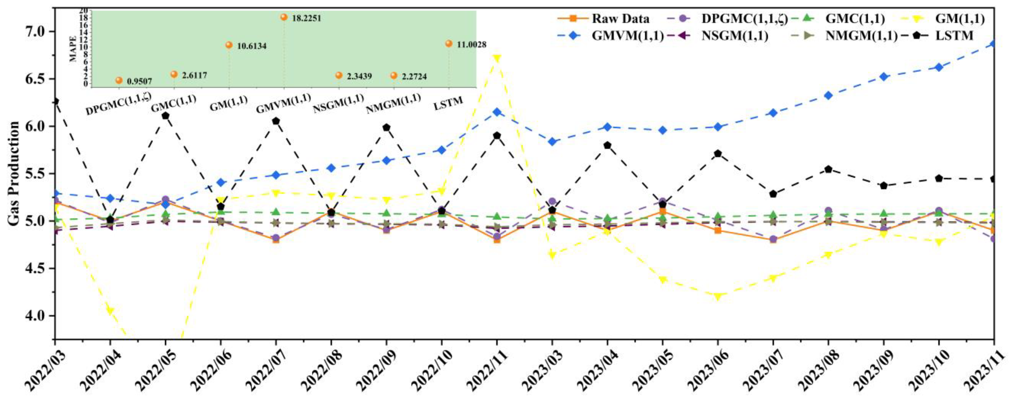
		DPGMC(1,1,ζ) ζ = 0.0178	GMC(1,1)	GM(1,1)	GMVM(1,1)	NSGM(1,1)	NMGM(1,1)	LSTM
Mar. 2021	5.6	5.6000	5.6000	5.6000	5.6000	5.6000	5.6000	4.5860
Apr. 2021	5.4	5.4000	5.3221	1.9171	5.3003	5.4420	5.6043	5.9785
May. 2021	5.5	5.5000	5.3027	4.7737	5.2531	5.3151	5.3132	4.5090
Jun. 2021	5.3	5.3000	5.2666	6.8709	5.2309	5.1924	5.1285	6.2710
Jul. 2021	5.4	5.4000	5.2309	6.6953	5.2087	5.1218	5.0441	4.5351
Aug. 2021	4.7	4.7000	5.2106	6.6617	5.2019	5.0701	4.9989	6.5843
Sep. 2021	4.4	4.4000	5.1794	7.5430	5.2437	5.0061	4.9543	4.9369
Oct. 2021	4.7	4.7000	5.1194	8.6381	5.3428	4.9279	4.9063	6.3443
Nov. 2021	5.1	5.1000	5.0469	8.2215	5.4148	4.8746	4.8854	4.8361
Mar. 2022	5.2	5.2211	5.0144	5.1461	5.2924	4.9015	4.9293	6.2642
Apr. 2022	5.0	4.9813	5.0312	4.0544	5.2393	4.9446	4.9720	5.0140
May. 2022	5.2	5.2277	5.0703	3.1641	5.1728	4.9963	5.0109	6.1109
Jun. 2022	5.0	5.0008	5.0937	5.2229	5.4071	4.9881	4.9935	5.1525
Jul. 2022	4.8	4.8233	5.0891	5.2986	5.4849	4.9789	4.9813	6.0543
Aug. 2022	5.1	5.0711	5.0827	5.2712	5.5599	4.9715	4.9743	5.0913
Sep. 2022	4.9	4.9099	5.0763	5.2260	5.6388	4.9661	4.9706	5.9866
Oct. 2022	5.1	5.1209	5.0687	5.3188	5.7489	4.9594	4.9665	5.1058
Nov. 2022	4.8	4.8377	5.0421	6.7273	6.1502	4.9219	4.9381	5.9004
Mar. 2023	5.1	5.2085	5.0224	4.6431	5.8386	4.9395	4.9599	5.1154
Apr. 2023	4.9	5.0095	5.0253	4.8921	5.9923	4.9475	4.9678	5.7983
May. 2023	5.1	5.2083	5.0312	4.3842	5.9578	4.9653	4.9815	5.1734
Jun. 2023	4.9	5.0088	5.0457	4.2087	5.9939	4.9831	4.9924	5.7112
Jul. 2023	4.8	4.8096	5.0604	4.3999	6.1411	4.9928	4.9952	5.2856
Aug. 2023	5.0	5.1101	5.0699	4.6470	6.3259	4.9948	4.9922	5.5445
Sep. 2023	4.9	4.9103	5.0738	4.8668	6.5241	4.9913	4.9864	5.3726
Oct. 2023	5.1	5.1103	5.0760	4.7834	6.6227	4.9904	4.9846	5.4490
Nov. 2023	4.9	4.8110	5.0761	5.0521	6.8713	4.9837	4.9787	5.4437
MAPE (%)		0.9507	2.6117	10.6134	18.2251	2.3439	2.2724	11.0028
MAE		0.0474	0.1288	0.5293	0.9009	0.1174	0.1137	0.5439
MSE		0.0040	0.0232	0.6023	1.0985	0.0188	0.0174	0.4775
$R^2$		0.7563	−0.4029	−35.4246	−65.4012	−0.1382	−0.0490	−27.8616
RMSE		0.0635	0.1523	0.7763	1.0481	0.1372	0.1317	0.6910

. According to Table 3, trend charts are drawn for the predicted data of six models as shown in Figure 2.

From Table 3, the four indicators of the DPGMC (1,1,ζ) model are optimal among the seven models. The MAPE of the four models PGMC (1,1), GMC (1,1), NSGM (1,1), and NMGM (1,1) are all below 5%; LSTM has a performance of 11.0028%, which is better than GMVM (1,1) and close to GM (1,1). Among them, the MAPE of DPGMC(1,1,ζ) is 0.9507%, which is much better than the simulation results of the other six models. The $R^2$ of the DPGMC (1,1,ζ) model is 0.7563, which is similar to 1. The overall fitting effect of the model is good, while other models show $R^2<0$, indicating that other models may have overfitting. Figure 2 shows the trend charts of seven models, from which it can be more intuitively seen that the original data overlaps with the DPGMC(1,1,ζ) simulation data, while the trends of other models have significant differences compared to the original data.

Case 2. Natural gas as the main sequence, and crude oil as the related sequence

Selecting natural gas and crude oil data from March to November each year from 2021 to 2023 as modelling objects, the simulated values and MAPE of DPGMC(1,N,ζ) and the comparative model were calculated, and the results are shown in

Table 4. Comparison results of six models for natural gas and crude oil in Case 2.

Month	${\mathit{X}}_1^{(0)}$	${\widehat{\mathit{X}}}_1^{(0)}$
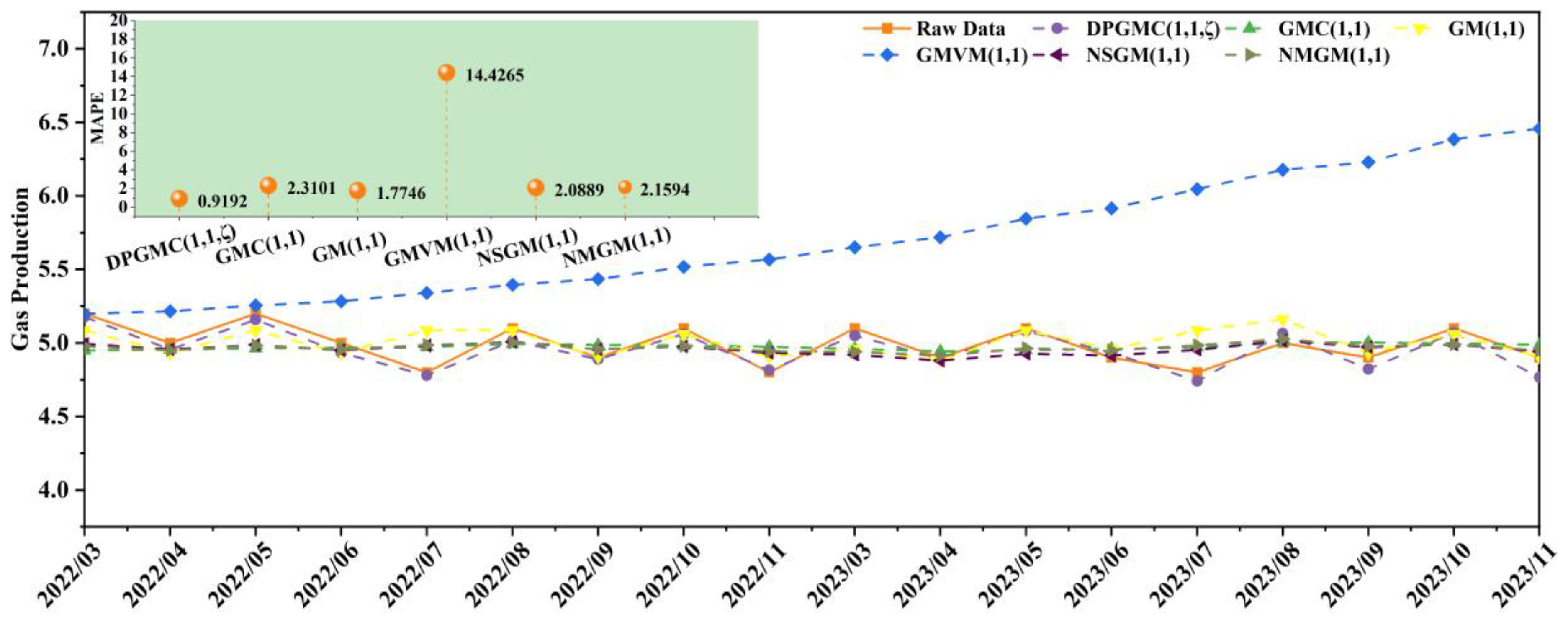
		DPGMC(1,1,ζ) ζ = 0.9000	GMC(1,1)	GM(1,1)	GMVM(1,1)	NSGM(1,1)	NMGM(1,1)
Mar. 2021	5.6	5.6000	5.6000	5.6000	5.6000	5.6000	5.6000
Apr. 2021	5.4	5.4000	4.8564	4.2758	5.2770	5.3342	5.5273
May. 2021	5.5	5.5000	4.8806	5.1209	5.2388	5.2693	5.2927
Jun. 2021	5.3	5.3000	4.8934	4.8830	5.2080	5.1501	5.1076
Jul. 2021	5.4	5.4000	4.9088	5.0590	5.1871	5.1268	5.0621
Aug. 2021	4.7	4.7000	4.9387	5.0589	5.1739	5.1087	5.0372
Sep. 2021	4.4	4.4000	4.9378	4.8810	5.1647	5.0257	4.9672
Oct. 2021	4.7	4.7000	4.9427	5.0589	5.1702	5.0304	4.9850
Nov. 2021	5.1	5.1000	4.9408	4.8810	5.1738	4.9651	4.9386
Mar. 2022	5.2	5.1762	4.9484	5.0843	5.1980	4.9933	4.9773
Apr. 2022	5.0	4.9555	4.9545	4.9318	5.2151	4.9560	4.9504
May. 2022	5.2	5.1586	4.9641	5.0843	5.2552	4.9863	4.9838
Jun. 2022	5.0	4.9320	4.9665	4.9318	5.2833	4.9506	4.9540
Jul. 2022	4.8	4.7799	4.9732	5.0843	5.3409	4.9821	4.9858
Aug. 2022	5.1	5.0143	4.9938	5.0843	5.3951	5.0065	5.0032
Sep. 2022	4.9	4.8891	4.9859	4.9064	5.4345	4.9564	4.9566
Oct. 2022	5.1	5.0602	4.9820	5.0589	5.5176	4.9767	4.9792
Nov. 2022	4.8	4.8149	4.9742	4.9064	5.5675	4.9334	4.9434
Mar. 2023	5.1	5.0503	4.9595	4.9572	5.6506	4.9195	4.9398
Apr. 2023	4.9	4.8916	4.9433	4.8810	5.7183	4.8792	4.9138
May. 2023	5.1	5.0821	4.9503	5.0843	5.8455	4.9267	4.9637
Jun. 2023	4.9	4.9338	4.9594	4.9572	5.9153	4.9143	4.9510
Jul. 2023	4.8	4.7403	4.9704	5.0843	6.0462	4.9540	4.9841
Aug. 2023	5.0	5.0638	5.0019	5.1606	6.1770	5.0143	5.0264
Sep. 2023	4.9	4.8218	5.0031	4.9318	6.2298	4.9723	4.9774
Oct. 2023	5.1	5.0698	4.9978	5.0589	6.3844	4.9890	4.9906
Nov. 2023	4.9	4.7660	4.9863	4.9064	6.4587	4.9429	4.9497
MAPE (%)		0.9192	2.3101	1.7746	14.4265	2.0889	2.1594
MAE		0.0458	0.1156	0.0878	0.7132	0.1048	0.1081
MSE		0.0031	0.0178	0.0147	0.7169	0.0154	0.0158
$R^2$		0.8147	−0.0752	0.1140	−42.3333	0.0684	0.0422
RMSE		0.0554	0.1334	0.1211	0.8467	0.1241	0.1259

. According to Table 4, draw trend charts for the predicted data of six models as shown in Figure 3.

From the data in Table 4, it can be concluded that the average absolute percentage error (MAPE) of the GMVM (1,1) model is 14.4265%, while the MAPE values of the other five models are all below 5%. Specifically, the MAPE of the DPGMC(1,1,ζ) model is only 0.9192%, indicating that the predictive performance of the DPGMC(1,1,ζ) model is the best. Additionally, its $R^2$ is also close to 1, indicating a good overall fitting effect. In the trend charts of the six models shown in Figure 3, it can be more intuitively seen that the original data overlaps with the DPGMC(1,1,ζ) simulation data. The GMVM (1,1) simulation data shows a linear upward trend, which is significantly different from the fluctuation of the original data. The trend charts of other models also have significant differences from the original data.

Case 3. Natural gas as the main sequence, and electric power generation as the related sequence.

Selecting natural gas and power generation data from March to November each year from 2021 to 2023 as the modelling objects, the simulated values and MAPE of DPGMC(1,N,ζ) and the comparative model were calculated, and the results are shown in

Table 5. Comparison results of six models for natural gas and electric power generation in Case 3.

Month	${\mathit{X}}_1^{(0)}$	${\widehat{\mathit{X}}}_1^{(0)}$
		DPGMC(1,1,ζ) ζ = 0.7151	GMC(1,1)	GM(1,1)	GMVM(1,1)	NSGM(1,1)	NMGM(1,1)
Mar. 2021	5.6	5.6000	5.6000	5.6000	5.6000	5.6000	5.6000
Apr. 2021	5.4	5.4000	5.3818	3.7821	5.2706	5.3673	5.5417
May. 2021	5.5	5.5000	5.3835	5.3309	5.2321	5.3095	5.3183
Jun. 2021	5.3	5.3000	5.4212	5.2045	5.2021	5.2453	5.1753
Jul. 2021	5.4	5.4000	5.4070	6.1805	5.1916	5.0820	5.0129
Aug. 2021	4.7	4.7000	5.3547	5.7842	5.1833	4.9836	4.9419
Sep. 2021	4.4	4.4000	5.3628	4.5831	5.1605	5.0195	4.9826
Oct. 2021	4.7	4.7000	5.4103	4.9346	5.1671	5.0141	4.9818
Nov. 2021	5.1	5.1000	5.4318	5.2750	5.1877	4.9764	4.9578
Mar. 2022	5.2	5.1762	5.4507	5.0087	5.1964	4.9718	4.9621
Apr. 2022	5.0	4.9577	5.4680	5.3772	5.2405	4.9321	4.9392
May. 2022	5.2	5.1451	5.4945	4.7903	5.2394	4.9571	4.9664
Jun. 2022	5.0	4.9336	5.5285	5.3021	5.3119	4.9275	4.9468
Jul. 2022	4.8	4.7812	5.5279	5.6501	5.3952	4.8696	4.9113
Aug. 2022	5.1	5.0219	5.5444	4.8586	5.3794	4.8998	4.9454
Sep. 2022	4.9	4.8754	5.6423	3.7872	5.3050	5.0288	5.0394
Oct. 2022	5.1	5.0449	5.7727	4.3672	5.4103	5.0769	5.0542
Nov. 2022	4.8	4.8085	5.8687	4.8381	5.5285	5.0699	5.0303
Mar. 2023	5.1	5.0635	5.9352	5.2339	5.6617	5.0256	4.9890
Apr. 2023	4.9	4.8939	5.9897	5.2339	5.7493	4.9898	4.9648
May. 2023	5.1	5.1080	6.0590	4.9882	5.7938	4.9846	4.9676
Jun. 2023	4.9	4.9283	6.1373	5.1793	5.9263	4.9618	4.9561
Jul. 2023	4.8	4.7343	6.1965	5.5955	6.1299	4.9027	4.9205
Aug. 2023	5.0	5.0432	6.2420	5.5955	6.2570	4.8548	4.8997
Sep. 2023	4.9	4.8406	6.3247	4.7903	6.1621	4.8944	4.9433
Oct. 2023	5.1	5.0804	6.4550	4.6880	6.2352	4.9366	4.9758
Nov. 2023	4.9	4.7653	6.5900	4.9541	6.4264	4.9448	4.9765
MAPE (%)		0.8624	18.4241	7.9274	14.1216	2.3354	2.3263
MAE		0.0430	0.9126	0.3934	0.6975	0.1170	0.1164
MSE		0.0028	1.0040	0.2438	0.6851	0.0193	0.0174
$R^2$		0.8307	−59.6868	−13.7351	−41.0168	−0.1651	−0.0527
RMSE		0.0529	1.0020	0.4937	0.8337	0.1388	0.1320

. According to Table 5, trend charts are drawn for the predicted data of six models as shown in Figure 4.

From Table 5, it can be seen that the MAPE of DPGMC(1,1,ζ), NSGM (1,1), and NMGM (1,1) models are all below 5%, with DPGMC(1,1,ζ) having a MAPE of only 0.8624%, indicating a significantly better predictive performance than the other five models. Although the MAPE of NSGM (1,1) and NMGM (1,1) are both below 5%, their $R^2$ is much smaller than 1, and the overall simulation effect of DPGMC(1,1,ζ) is better. In the trend charts of the six models shown in Figure 4, it can more intuitively be observed that the original data almost completely overlaps with the DPGMC(1,1,ζ) simulation data. In contrast, the lines simulated by GMC (1,1) and GMVM (1,1) models both show a linear upward trend, which is significantly different from the fluctuations of the original data. The fluctuation amplitude of the GM (1,1) model is relatively large, while the fluctuation amplitudes of the NSGM (1,1) and NMGM (1,1) models are relatively small, but they still cannot fully match the fluctuations of the original data.

4.2. Effectiveness Analysis of the Second Category DPGMC(1,N,ζ)

This section focuses on natural gas production as the main characteristic sequence and combines raw coal, crude oil, and power generation in pairs to form different related sequence combinations for effectiveness analysis. It is divided into three cases, as follows:

Case 4. Natural gas as the main sequence, with raw coal and crude oil as related sequences.

Selecting natural gas, raw coal, and crude oil data from March to November each year from 2021 to 2023 as the modelling objects, 18 natural gas data from 2022 to 2023 were used to test the effectiveness of the model. The simulated values and MAPE of DPGMC(1,N,ζ) and the comparative model were calculated, and the results are shown in

Table 6. Comparison results of six models with raw coal and crude oil as related sequences in Case 4.

Month	${\mathit{X}}_1^{(0)}$	${\widehat{\mathit{X}}}_1^{(0)}$
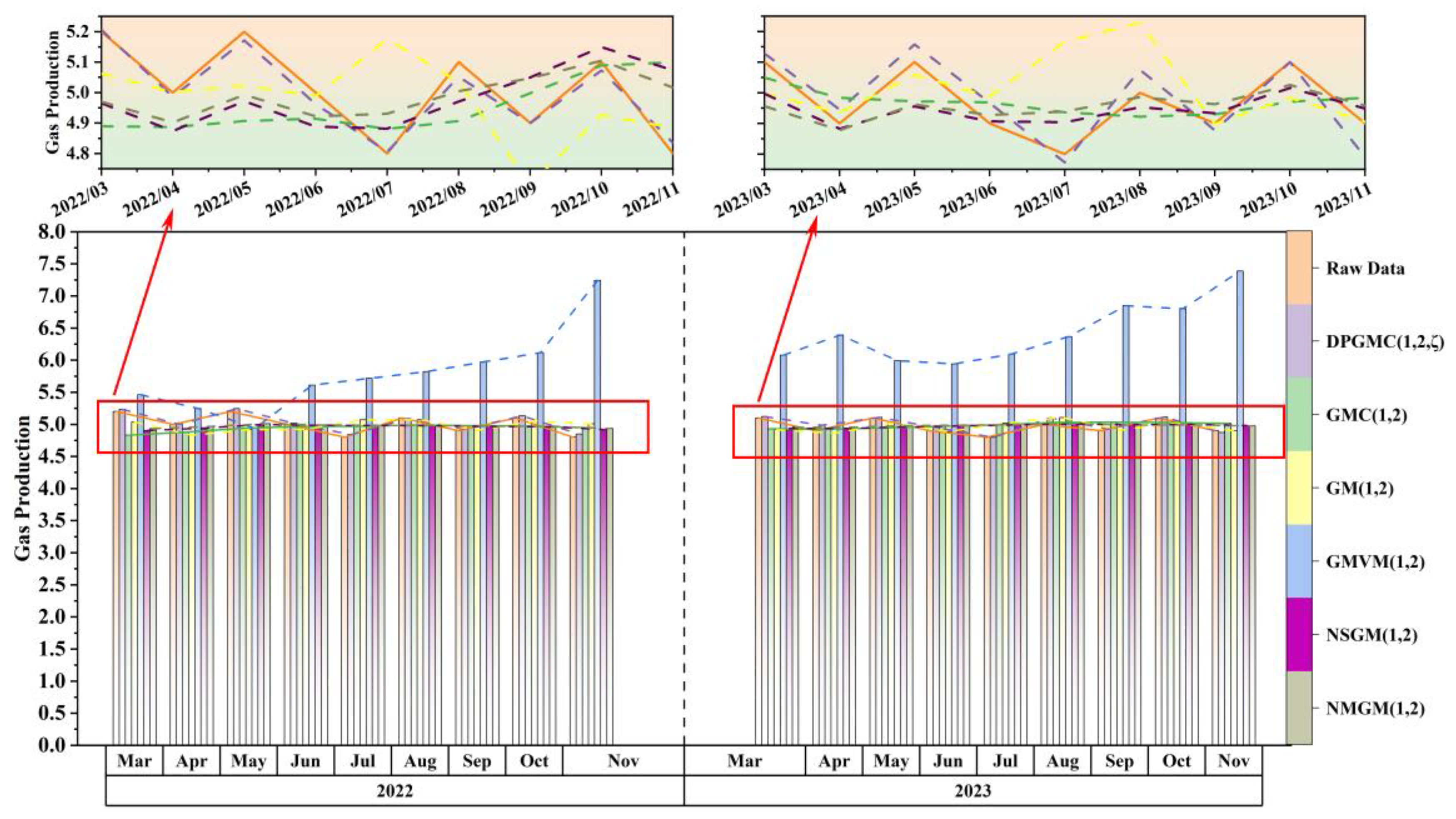
		DPGMC(1,2,ζ) ζ = 0.8734	GMC(1,2)	GM(1,2)	GMVM(1,2)	NSGM(1,2)	NMGM(1,2)
Mar. 2021	5.6	5.6000	5.6000	5.6000	5.6000	5.6000	5.6000
Apr. 2021	5.4	5.4000	5.0003	4.2089	5.3210	5.4388	5.6012
May. 2021	5.5	5.5000	4.9732	5.2639	5.2600	5.3175	5.3160
Jun. 2021	5.3	5.3000	4.9329	5.0249	5.2614	5.1875	5.1240
Jul. 2021	5.4	5.4000	4.9091	5.1014	5.2382	5.1229	5.0459
Aug. 2021	4.7	4.7000	4.9198	5.0895	5.2459	5.0756	5.0043
Sep. 2021	4.4	4.4000	4.8962	4.9931	5.3993	5.0034	4.9510
Oct. 2021	4.7	4.7000	4.8589	5.2409	5.6992	4.9324	4.9104
Nov. 2021	5.1	5.1000	4.8177	5.0514	5.9142	4.8718	4.8820
Mar. 2022	5.2	5.2356	4.8299	5.0367	5.4608	4.9050	4.9324
Apr. 2022	5.0	4.9979	4.8788	4.8302	5.2478	4.9413	4.9684
May. 2022	5.2	5.2430	4.9390	4.9192	4.9400	4.9979	5.0126
Jun. 2022	5.0	5.0176	4.9660	4.9219	5.6115	4.9845	4.9901
Jul. 2022	4.8	4.8393	4.9707	5.0719	5.7166	4.9821	4.9849
Aug. 2022	5.1	5.0903	4.9883	5.0724	5.8207	4.9800	4.9818
Sep. 2022	4.9	4.9238	4.9804	4.9056	5.9710	4.9662	4.9689
Oct. 2022	5.1	5.1334	4.9744	5.0548	6.1166	4.9638	4.9694
Nov. 2022	4.8	4.8470	4.9489	5.0084	7.2429	4.9200	4.9349
Mar. 2023	5.1	5.1215	4.9303	4.9163	6.0758	4.9346	4.9550
Apr. 2023	4.9	4.9847	4.9268	4.8626	6.3920	4.9350	4.9571
May. 2023	5.1	5.1087	4.9451	5.0178	5.9908	4.9608	4.9803
Jun. 2023	4.9	4.9503	4.9705	4.8881	5.9415	4.9758	4.9883
Jul. 2023	4.8	4.7979	4.9933	5.0192	6.0961	4.9925	4.9977
Aug. 2023	5.0	5.0994	5.0289	5.1067	6.3659	5.0055	5.0036
Sep. 2023	4.9	4.9263	5.0318	4.9089	6.8499	4.9947	4.9884
Oct. 2023	5.1	5.1124	5.0261	5.0215	6.8014	4.9970	4.9893
Nov. 2023	4.9	4.8727	5.0130	4.8978	7.3875	4.9822	4.9752
MAPE (%)		0.6530	2.6438	2.2076	23.3142	2.3165	2.2437
MAE		0.0325	0.1326	0.1101	1.1527	0.1161	0.1122
MSE		0.0017	0.0244	0.0205	1.7536	0.0185	0.0171
$R^2$		0.8970	−0.4751	−0.2371	−105.0031	−0.1202	−0.0317
RMSE		0.0413	0.1562	0.1431	1.3242	0.1361	0.1306

. According to Table 6, trend charts are drawn for the predicted data of six models as shown in Figure 5.

From Table 6, it can be seen that the DPGMC(1,2,ζ) model has the best performance, with a MAPE of only 0.6530%. In contrast, GMVM (1,2) performs the worst. The values of the other four types of MAPE are around 2%. Overall, DPGMC(1,2,ζ) has a good fitting effect. The trend charts of the six models in Figure 5 more intuitively reflect the effectiveness of the models. In the lower part of Figure 5, it can be observed there are significant differences between the GMVM (1,2) and the original data. Furthermore, in the enlarged image of Figure 5, it can be seen that the DPGMC(1,2,ζ) model almost completely overlaps with the original data, while other models have some differences from the original data.

Case 5. Natural gas as the main sequence, with raw coal and electric power generation as related sequences

Selecting natural gas, raw coal, and power generation data from March to November each year from 2021 to 2023 as the modelling objects, the simulated values and MAPE of DPGMC(1,N,ζ) and the comparative model were calculated. The results are shown in

Table 7. Comparison results of six models with related sequences of raw coal and electric power generation in Case 5.

Month	${\mathit{X}}_1^{(0)}$	${\widehat{\mathit{X}}}_1^{(0)}$
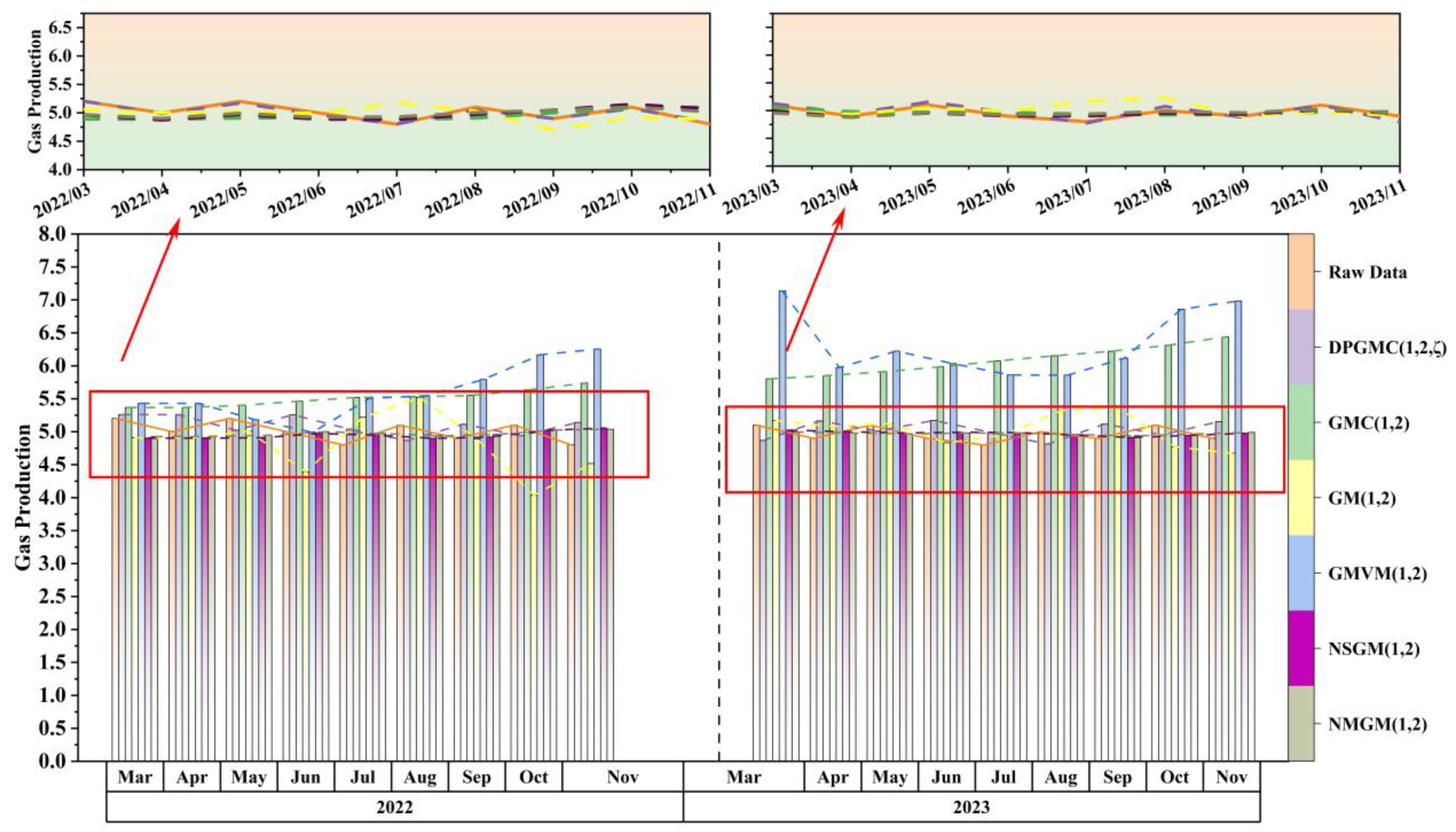
		DPGMC(1,2,ζ) ζ = 0.6213	GMC(1,2)	GM(1,2)	GMVM(1,2)	NSGM(1,2)	NMGM(1,2)
Mar. 2021	5.6	5.6000	5.6000	5.6000	5.6000	5.6000	5.6000
Apr. 2021	5.4	5.4000	5.4719	3.3740	5.3189	5.4456	5.6010
May. 2021	5.5	5.5000	5.4715	5.5741	5.2632	5.3542	5.3438
Jun. 2021	5.3	5.3000	5.4834	5.8037	5.2615	5.2487	5.1658
Jul. 2021	5.4	5.4000	5.4570	6.2538	5.2171	5.0943	5.0156
Aug. 2021	4.7	4.7000	5.4158	5.8223	5.2126	4.9984	4.9470
Sep. 2021	4.4	4.4000	5.4096	5.0243	5.3805	4.9945	4.9539
Oct. 2021	4.7	4.7000	5.4072	5.5266	5.6485	4.9426	4.9209
Nov. 2021	5.1	5.1000	5.3732	5.7196	5.8065	4.8801	4.8884
Mar. 2022	5.2	5.2598	5.3676	4.9060	5.4310	4.9025	4.9281
Apr. 2022	5.0	5.0225	5.4018	5.0076	5.1809	4.9089	4.9466
May. 2022	5.2	5.2562	5.4628	4.3851	4.9910	4.9732	5.0006
Jun. 2022	5.0	5.0385	5.5195	5.2172	5.5049	4.9486	4.9736
Jul. 2022	4.8	4.8683	5.5293	5.5186	5.5480	4.8995	4.9371
Aug. 2022	5.1	5.1159	5.5509	4.8901	5.7919	4.9207	4.9574
Sep. 2022	4.9	4.9391	5.6322	4.0335	6.1672	5.0212	5.0268
Oct. 2022	5.1	5.1402	5.7367	4.5169	6.2535	5.0562	5.0358
Nov. 2022	4.8	4.8658	5.8016	5.1721	7.1353	5.0236	4.9950
Mar. 2023	5.1	5.1670	5.8501	5.0770	5.9739	5.0025	4.9803
Apr. 2023	4.9	5.0092	5.9097	5.1274	6.2233	4.9808	4.9678
May. 2023	5.1	5.1714	5.9840	4.8325	6.0322	4.9909	4.9809
Jun. 2023	4.9	4.9893	6.0738	4.9505	5.8608	4.9874	4.9811
Jul. 2023	4.8	4.8118	6.1524	5.3199	5.8574	4.9489	4.9562
Aug. 2023	5.0	5.1194	6.2194	5.3689	6.1158	4.9133	4.9376
Sep. 2023	4.9	4.9502	6.3112	4.7718	6.8594	4.9428	4.9661
Oct. 2023	5.1	5.1529	6.4382	4.6740	6.9831	4.9762	4.9898
Nov. 2023	4.9	4.8786	6.5692	4.9389	7.2853	4.9781	4.9858
MAPE (%)		1.1135	17.6279	6.8397	22.2456	2.4293	2.3169
MAE		0.0555	0.8728	0.3408	1.1007	0.1216	0.1158
MSE		0.0039	0.9352	0.1844	1.6421	0.0193	0.0170
$R^2$		0.7623	−55.5327	−10.1480	−98.2617	−0.1689	−0.0291
RMSE		0.0627	0.9671	0.4294	1.2814	0.1391	0.1305

. According to Table 7, trend charts are drawn for the predicted data of six models as shown in Figure 6.

From Table 7, it can be seen that from these five indicators, it is evident that DPGMC(1,2,ζ) has a good effect. The MAPE of DPGMC(1,2,ζ), NSGM (1,2), and NMGM (1,2) models are all below 5%. Among them, the MAPE of DPGMC(1,2,ζ) is only 1.1135%, which is much better than the simulation results of the other five models. In contrast, the MAPE values of GMC (1,2) and GMVM (1,2) models are higher, at 17.6279% and 22.2456%, respectively. The trend charts of the six models in Figure 6 more intuitively reflect the effectiveness of the models. It can be observed that the GMC (1,2) and GMVM (1,2) models have significant differences from the original data, and from the enlarged image in Figure 6, it can be found that the DPGMC(1,2,ζ) model overlaps with the original data. The fluctuation amplitude of the NSGM (1,2) and NMGM (1,2) models is roughly the same as that of the original data, but other models have certain differences from the original data.

Case 6. Natural gas as the main sequence, with crude oil and electric power generation as related sequences.

Selecting natural gas, crude oil, and power generation data from March to November each year from 2021 to 2023 as modelling objects, the simulated values and MAPE of DPGMC(1,N,ζ) and the comparative model were calculated, and the results are shown in

Table 8. Comparison results of six models with correlation sequences between crude oil and electric power generation in Case 6.

Month	${\mathit{X}}_1^{(0)}$	${\widehat{\mathit{X}}}_1^{(0)}$
		DPGMC(1,2,ζ) ζ = 0.4363	GMC(1,2)	GM(1,2)	GMVM(1,2)	NSGM(1,2)	NMGM(1,2)
Mar. 2021	5.6	5.6000	5.6000	5.6000	5.6000	5.6000	5.6000
Apr. 2021	5.4	5.4000	5.0016	4.2726	5.2852	5.3840	5.5468
May. 2021	5.5	5.5000	4.9679	5.0992	5.2560	5.3742	5.3696
Jun. 2021	5.3	5.3000	4.9701	4.8934	5.2252	5.2243	5.1514
Jul. 2021	5.4	5.4000	4.9009	5.2378	5.1370	5.0864	5.0153
Aug. 2021	4.7	4.7000	4.8372	5.1756	5.0911	5.0140	4.9633
Sep. 2021	4.4	4.4000	4.8439	4.8180	5.1755	4.9744	4.9398
Oct. 2021	4.7	4.7000	4.8912	5.0271	5.1695	5.0204	4.9900
Nov. 2021	5.1	5.1000	4.8846	4.9421	5.0545	4.8971	4.8953
Mar. 2022	5.2	5.2054	4.8899	5.0613	5.1767	4.9652	4.9702
Apr. 2022	5.0	4.9861	4.8863	5.0020	5.0031	4.8739	4.9017
May. 2022	5.2	5.1713	4.9067	5.0224	5.3136	4.9719	4.9931
Jun. 2022	5.0	4.9622	4.9145	4.9886	5.0297	4.8884	4.9221
Jul. 2022	4.8	4.8054	4.8807	5.1757	4.8970	4.8819	4.9305
Aug. 2022	5.1	5.0522	4.9063	5.0346	5.4149	4.9704	5.0046
Sep. 2022	4.9	4.8996	4.9980	4.6977	6.2207	5.0496	5.0474
Oct. 2022	5.1	5.0727	5.0891	4.9261	6.1322	5.1496	5.1046
Nov. 2022	4.8	4.8351	5.0995	4.8850	5.7034	5.0726	5.0164
Mar. 2023	5.1	5.1278	5.0490	4.9973	5.4233	4.9968	4.9558
Apr. 2023	4.9	4.9455	4.9837	4.9348	5.3394	4.8825	4.8781
May. 2023	5.1	5.1576	4.9718	5.0577	6.0024	4.9555	4.9616
Jun. 2023	4.9	4.9664	4.9686	4.9876	5.6272	4.9067	4.9273
Jul. 2023	4.8	4.7729	4.9363	5.1660	5.2298	4.9035	4.9384
Aug. 2023	5.0	5.0747	4.9219	5.2285	5.3558	4.9525	4.9861
Sep. 2023	4.9	4.8775	4.9295	4.8974	6.4082	4.9332	4.9624
Oct. 2023	5.1	5.1000	4.9708	4.9833	7.0872	5.0156	5.0252
Nov. 2023	4.9	4.7903	4.9833	4.9057	6.3451	4.9484	4.9582
MAPE (%)		0.7072	2.5213	2.4869	13.3693	2.1880	2.0976
MAE		0.0352	0.1263	0.1233	0.6642	0.1096	0.1048
MSE		0.0020	0.0237	0.0275	0.7785	0.0174	0.0155
$R^2$		0.8785	−0.4299	−0.6649	−46.0577	−0.0531	0.0615
RMSE		0.0448	0.1538	0.1660	0.8823	0.1320	0.1246

. According to Table 8, trend charts are drawn for the predicted data of six models as shown in Figure 7.

From Table 8, it can be seen that the MAPE of the DPGMC(1,2,ζ) model is 0.7072%, indicating the best performance. In contrast, the GMVM (1,2) model has the worst performance, with a MAPE value of up to 13.3693%. The other four grey models have similar effects, with MAPE values around 2%. Meanwhile, based on these four indicators, it is evident that DPGMC(1,2,ζ) has a good effect. The trend charts of the six models in Figure 7 more intuitively reflect the effectiveness of the models. It can be observed from the figures that there are significant differences between the GMVM (1,2) model and the original data. In the enlarged image in Figure 7, it can be seen that the trend of the DPGMC(1,2,ζ) model is consistent with the original data. Although the GMC (1,2), NSGM (1,2), and NMGM (1,2) models have roughly the same trend as the original data, the data simulated by the GM (1,2) model fluctuates greatly and has significant differences from the original data.

4.3. Effectiveness Analysis of the Third Category DPGMC(1,N,ζ)

Case 7. Selecting the natural gas production from March to November each year from 2021 to 2023 as the main feature sequence, the effectiveness analysis was conducted on the three related sequences of raw coal, crude oil, and electric power generation. The simulated values and MAPE of DPGMC(1,N,ζ) and the comparative model were calculated, and the results are shown in

Table 9. Comparison results of six models related to the third type of raw coal, crude oil, and electric power generation sequences.

Month	${\mathit{X}}_1^{(0)}$	${\widehat{\mathit{X}}}_1^{(0)}$
		DPGMC(1,3,ζ) ζ = 0.9900	GMC(1,3)	GM(1,3)	GMVM(1,3)	NSGM(1,3)	NMGM(1,3)
Mar. 2021	5.6	5.6000	5.6000	5.6000	5.6000	5.6000	5.6000
Apr. 2021	5.4	5.4000	5.0734	4.2107	5.3169	5.4243	5.5829
May. 2021	5.5	5.5000	5.0184	5.2433	5.2642	5.3824	5.3694
Jun. 2021	5.3	5.3000	4.9901	5.0157	5.2599	5.2324	5.1535
Jul. 2021	5.4	5.4000	4.9095	5.1678	5.2066	5.0926	5.0165
Aug. 2021	4.7	4.7000	4.8462	5.1325	5.1962	5.0145	4.9596
Sep. 2021	4.4	4.4000	4.8345	4.9569	5.3640	4.9728	4.9356
Oct. 2021	4.7	4.7000	4.8469	5.2098	5.6078	4.9779	4.9483
Nov. 2021	5.1	5.1000	4.8149	5.0582	5.7339	4.8635	4.8710
Mar. 2022	5.2	5.2238	4.8217	5.0325	5.4092	4.9267	4.9451
Apr. 2022	5.0	4.9915	4.8455	4.8682	5.1519	4.8759	4.9181
May. 2022	5.2	5.2089	4.8953	4.9115	5.0251	4.9765	5.0058
Jun. 2022	5.0	5.0082	4.9183	4.9453	5.4484	4.9108	4.9473
Jul. 2022	4.8	4.8182	4.8896	5.1092	5.4635	4.8955	4.9408
Aug. 2022	5.1	5.0906	4.9118	5.0540	5.7654	4.9629	4.9931
Sep. 2022	4.9	4.8925	4.9881	4.8234	6.2331	5.0395	5.0370
Oct. 2022	5.1	5.1072	5.0653	5.0028	6.2924	5.1176	5.0764
Nov. 2022	4.8	4.8299	5.0644	4.9896	7.0310	5.0450	4.9984
Mar. 2023	5.1	5.0779	5.0188	4.9363	5.9176	4.9909	4.9609
Apr. 2023	4.9	4.9408	4.9698	4.8857	6.1296	4.9064	4.9083
May. 2023	5.1	5.1072	4.9679	5.0140	6.0482	4.9669	4.9718
Jun. 2023	4.9	4.9078	4.9770	4.9071	5.8288	4.9364	4.9527
Jul. 2023	4.8	4.7862	4.9588	5.0580	5.7566	4.9298	4.9554
Aug. 2023	5.0	5.0431	4.9532	5.1390	6.0054	4.9595	4.9823
Sep. 2023	4.9	4.9376	4.9596	4.8976	6.8459	4.9506	4.9712
Oct. 2023	5.1	5.1095	4.9930	4.9954	7.0521	5.0171	5.0183
Nov. 2023	4.9	4.8625	5.0012	4.8984	7.2136	4.9670	4.9705
MAPE (%)		0.3821	2.6781	2.3823	21.5136	2.2198	2.1290
MAE		0.0189	0.1343	0.1188	1.0649	0.1111	0.1064
MSE		0.0005	0.0265	0.0229	1.5653	0.0177	0.0157
$R^2$		0.9683	−0.5996	−0.3883	−93.6203	−0.0716	0.0533
RMSE		0.0229	0.1627	0.1513	1.2511	0.1331	0.1251

. According to Table 9, trend charts are drawn for the predicted data of six models as shown in Figure 8.

It can be seen from Table 9 that the DPGMC(1,3,ζ) model performs the best, with an average absolute percentage error (MAPE) of only 0.3821%. In contrast, the GMVM (1,3) model performed the worst, with a MAPE value of up to 21.5136%. The $R^2$ of DPGMC(1,3,ζ) is 0.9683, close to 1, and the MAE, MSE, and RMSE are all small, indicating that the model has a good fitting effect. The trend charts of the six models in Figure 8 more intuitively reflect the effectiveness of the models. It can be observed from the figure that the DPGMC(1,3,ζ) model overlaps with the original data, and the error area is almost invisible, indicating that its simulation accuracy is very high. However, the error regions between other models and the original data are more obvious, indicating that their simulation accuracy is relatively low. Therefore, Figure 8 further confirms that the simulation accuracy of the DPGMC(1,3,ζ) model is superior to other models.

4.4. Summary of Effectiveness Analysis of Three Categories of DPGMC(1,N,ζ)

This section focuses on natural gas production as the main feature sequence. Based on the number and types of related variables, the relevant sequences are divided into three categories, and the effectiveness of the model is studied. From a horizontal comparison, the results of the DPGMC(1,3,ζ) model in seven cases of three types all indicate that its performance is far superior to the other five grey prediction models. Specifically, the MAPE values simulated by the DPGMC(1,3,ζ) model did not exceed 2%, achieving excellent results. This indicates that the simulation results of the partial grey prediction model have significantly improved compared to the classical ordinary differential grey prediction model. This is mainly because the biased grey prediction model considers the spatiotemporal nature of the data, which has a good effect on improving the accuracy of the model.

From a longitudinal perspective, this article mainly uses simulation results of natural gas production to demonstrate the effectiveness of the DPGMC(1,3,ζ) model. During this process, raw coal production, crude oil production, and electric power generation, which are closely related to natural gas production, are used as correlation sequences and modelled based on the number of related variables. The results showed that with the increase of relevant variables, the simulation accuracy of the DPGMC(1,N,ζ) model remained relatively stable and improved to some extent. This indicates that the DPGMC(1,N,ζ) model has strong stability and can effectively predict future natural gas production. Therefore, the DPGMC(1,3,ζ) model and its extended form DPGMC(1,N,ζ) have high application value in natural gas production prediction.

5. Application of DPGMC(1,N,ζ)

Based on the effectiveness analysis of the previous four sections, this section determines the optimal fitting effect of the DPGMC(1,3,ζ) model in natural gas production prediction. Therefore, this section applies the model to predict natural gas production. However, due to the limited number of available data, to reduce the possibility of significant errors in subsequent predictions, it was decided to supplement the four variables of natural gas production, raw coal production, crude oil production, and power generation with nine data points from March to November 2020, and combine them with the modelling objects in Section 4.3 to obtain the complete original dataset from 2020 to 2023. Subsequently, the DPGMC(1,3,ζ) model was used to predict the dataset, with the prediction results rounded to four decimal places. In data prediction, the GM (1,1) model and the Vurhulst model are first used to make preliminary predictions on the data, and these predicted values are used as inputs and combined into the DPGMC(1,3,ζ) model. The final predicted value is calculated based on the parameters obtained by DPGMC(1,3,ζ). The predicted results are shown in

Table 10. Prediction of natural gas production in Qinghai Province from March to November 2024.

Month	3	4	5	6	7	8	9	10	11
Nature Gas Production	7.6703	7.0827	7.3308	7.3726	7.2158	7.1693	7.2791	7.5310	7.3757

. To compare more intuitively with the previous data, a natural gas production forecast chart for 2020–2024 is drawn here, as shown in Figure 9.

From the predicted results in Table 10 and Figure 9, it can be further observed that the natural gas production in Qinghai Province in 2024 is relatively stable, and its trend is consistent with the previous four years, but overall, it has slightly increased compared to the previous four years. According to statistical data, the overall natural gas production in Qinghai Province has remained at a relatively high level in recent years. With the continuous advancement of natural gas exploration technology, extraction efficiency has been improved, and new natural gas reserves have also been discovered, making the Qaidam Basin one of the main natural gas enrichment areas in China. Due to the national strategy of vigorously developing a green ecological economy, the demand for natural gas as a clean energy source continues to increase. As an important energy base in the northwest region, the increase in natural gas production in Qinghai Province will help meet market demand and promote the sustainable development of the regional economy. Therefore, the overall natural gas production in 2024 is slightly higher than in previous years, and although there were fluctuations in monthly production between March and November, this is consistent with the fluctuations in data from previous years.

According to the prediction results in Table 10 and Figure 9, it can be found that there will be a production peak in March, May, August, and October each year, which is related to the weather in Qinghai Province and consistent with the actual situation. Therefore, the following suggestions are proposed for the prediction of natural gas production in Qinghai Province:

(1)

Dynamically adjust production plans and conduct equipment maintenance in advance from January to February before peak periods occur in these months to ensure that production equipment is in optimal condition during peak months. At the same time, utilise low season months to conduct in-depth maintenance and technological upgrades on equipment. Improve the efficiency of natural gas exploration, control open costs, and optimise development plans.

(2)

Data-driven decision-making, dynamically guiding and adjusting production strategies based on forecast results, establishing emergency data-driven mechanisms with surrounding provinces, coordinating exports in months of excess production, and complementing supply in months of shortage. At the same time, responding to seasonal fluctuations in natural gas demand based on forecast results, enhancing natural gas peak shaving capabilities, and ensuring stable supply.

(3)

Promote the complementary and coordinated development of natural gas and other energy sources. With the development of clean energy in Qinghai Province, the proportion of natural gas in the energy structure may change. Therefore, the energy structure should be adjusted promptly according to market demand, and the production forecast results provide an important basis for the development planning and investment decisions of the shale gas industry.

6. Conclusions

This paper combines the principle of fractional order accumulation with the partial grey prediction model to construct a fractional order partial grey DPGMC(1,N,ζ) model with spatiotemporal characteristics. This model extends the traditional grey prediction model from a single time-series input metadata to a matrix-structured partial grey prediction model. By introducing the damping fractional order principle and effectively representing the fractional order principle in a matrix, the grey prediction model is improved from both the model structure and the prediction object, significantly enhancing the stability and prediction accuracy of the model. In empirical research, the DPGMC(1,N,ζ) model was applied to predict natural gas production in Qinghai Province, China, and its effectiveness was analysed through seven cases in three directions. The results showed that the MAPE of these seven cases were all below 2%, indicating that the model has high prediction accuracy. Compared with the five classic and optimized grey prediction models, the DPGMC(1,N,ζ) model performs much better than other models. Based on the results of the effectiveness analysis, the best-performing case was selected to predict natural gas production for the next nine months, and the prediction results were analysed in depth. On this basis, we have put forward relevant policy recommendations and provided references for the sustainable development of the natural gas industry in Qinghai Province.

The grey DPGMC(1,N,ζ) model proposed in this article demonstrates high accuracy in natural gas prediction and effectively predicts future natural gas production, but there is still room for improvement. For example, in the context of policy changes, technological innovation, or market environment, establish corresponding grey prediction models, and combine them with this model using methods with long-term forecasting to demonstrate the reliability of the model in long-term forecasting. Apply the model to natural gas datasets from different regions to explore their adaptability and performance differences under different geographical, economic, or energy structure conditions, while simultaneously discussing the performance of the model on long-term or highly volatile data, as well as its utility and impact in strategic planning, to expand the application scope of the model. These will be important directions for future research.

References

- Liu, H.; Liang, K.; Zhang, G.S.; Li, Z.; Ding, L.; Su, J.; Zhu, S.; Ge, S.; Liu, J. Research on the development strategy of Chinese natural gas under the constraint of carbon peaking and carbon neutral. Strateg. Study CAE 2021, 23, 33. [Google Scholar] [CrossRef]
- Zou, C.; Zhao, Q.; Chen, J.; Li, J.; Yang, Z.; Sun, Q.; Lu, J.; Zhang, G. Natural gas in China: Development trend and strategic forecast. Nat. Gas Ind. B 2018, 5, 380–390. [Google Scholar] [CrossRef]
- Chen, Y.Q.; Fu, L.B.; Xu, J.Q. Application and comparison of two production decline models in shale gas wells and tight gas wells. Pet. Geol. Recovery Effic. 2021, 28, 6. [Google Scholar] [CrossRef]
- Chen, Y.R.; Yu, G.; Zou, Y.H.; Fang, Y. Optimization of natural gas production prediction method based on index and multiple correction coefficient. Nat. Gas Technol. Econ. 2021, 15, 83. [Google Scholar] [CrossRef]
- Chen, J.S.; Cao, J.Z.; Han, H.B.; Nian, J.; Guo, L. Adaptability analysis of commonly used production prediction models for shale oil and gas well. Unconv. Oil Gas 2019, 6, 48–57. [Google Scholar] [CrossRef]
- Wang Yu Li, Z.P.; Liu, C. Prediction for coal bed gas output based on fractal and ARIMA. Nat. Gas Oil 2011, 29, 45–48+87. [Google Scholar] [CrossRef]
- Manowska, A.; Rybak, A.; Dylong, A.; Pielot, J. Forecasting of natural gas consumption in pol and based on ARIMA-LSTM hybrid model. Energies 2021, 14, 8597. [Google Scholar] [CrossRef]
- Chen, Y.; Jiang, S.; Zhang, D.; Liu, C. An adsorbed gas estimation model for shale gas reservoirs via statistical learning. Appl. Energy 2017, 197, 327–341. [Google Scholar] [CrossRef]
- Smajla, I.; Vulin, D.; Sedlar, D.K. Short-term forecasting of natural gas consumption by determining the statistical distribution of consumption data. Energy Rep. 2023, 10, 2352–2360. [Google Scholar] [CrossRef]
- Kani, A.H.; Abbasspour, M.; Abedi, Z. Estimation of demand function for natural gas in Iran: Evidences based on smooth transition regression models. Econ. Model. 2014, 36, 341–347. [Google Scholar] [CrossRef]
- Zhou, Q.Q.; Duan, H.M.; Xie, D.R. A multivariate partial grey prediction model based on second-order traffic flow kinematics equation and its application. J. Comput. Appl. Math. 2025, 463, 116505. [Google Scholar] [CrossRef]
- Ji, L.; Li, J.H.; Xiao, J.L. Application of random forest algorithm in the multistage fracturing stimulation of shale gas field. Pet. Geol. Oilfield Dev. Daqing 2020, 39, 168–174. [Google Scholar] [CrossRef]
- Qiao, W.; Liu, W.; Liu, E. A combination model based on wavelet transform for predicting the difference between monthly natural gas production and consumption of U.S. Energy 2021, 235, 121216. [Google Scholar] [CrossRef]
- Zhu, H.; Kong, D.Q.; Qian, X. Method for predicting shale gas production based on ATD-BP neural network. Sci. Technol. Eng. 2017, 17, 128–132. [Google Scholar] [CrossRef]
- Zha, W.; Liu, Y.; Wan, Y.; Luo, R.; Li, D.; Yang, S.; Xu, Y. Forecasting monthly gas field production based on the CNN-LSTM model. Energy 2022, 260, 124889. [Google Scholar] [CrossRef]
- Anđelković, A.S.; Bajatović, D. Integration of weather forecast and artificial intelligence for a short-term city-scale natural gas consumption prediction. J. Clean. Prod. 2020, 266, 122096. [Google Scholar] [CrossRef]
- Chen, R.X.; Xiao, X.P.; Gao, M.Y.; Ding, Q. A novel mixed frequency sampling discrete grey model for forecasting hard disk drive failure. ISA Trans. 2024, 147, 304–327. [Google Scholar] [CrossRef]
- Li, X.M.; Li, N.; Ding, S.; Cao, Y.; Li, Y. A novel data-driven seasonal multivariable grey model for seasonal time series forecasting. Inf. Sci. 2023, 642, 119165. [Google Scholar] [CrossRef]
- Ye, L.L.; Xie, N.M.; Boylan, J.E.; Shang, Z. Forecasting seasonal demand for retail: A Fourier time-varying grey model. Int. J. Forecast. 2024, 40, 1467–1485. [Google Scholar] [CrossRef]
- Zeng, B.; Li, H.; Mao, C.W.; Wu, Y. Modeling, prediction and analysis of new energy vehicle sales in China using a variable-structure grey model. Expert Syst. Appl. 2023, 213, 118879. [Google Scholar] [CrossRef]
- Wang, Y.; Yang, Z.S.; Ye, L.L.; Wang, L.; Zhou, Y.; Luo, Y. A novel self-adaptive fractional grey Euler model with dynamic accumulation order and its application in energy production prediction of China. Energy 2023, 265, 126384. [Google Scholar] [CrossRef]
- Duan, H.M.; Wang, G.; Song, Y.X.; Chen, H. A novel grey multivariable time-delayed model and its application in predicting oil production. Eng. Appl. Artif. Intell. 2024, 139, 109505. [Google Scholar] [CrossRef]
- Wang, J.J.; Ye, L.; Ding, X.Y.; Dang, Y. A novel seasonal grey prediction model with time-lag and interactive effects for forecasting the photovoltaic power generation. Energy 2024, 304, 131939. [Google Scholar] [CrossRef]
- Zhang, R.Y.; Mao, S.Y.; Kang, Y.X. A novel traffic flow prediction model: Variable order fractional grey model based on an improved grey evolution algorithm. Expert Syst. Appl. 2023, 224, 119943. [Google Scholar] [CrossRef]
- Zhao, K.; Yu, S.J.; Wang, L.F. Carbon emissions prediction considering environment protection investment of 30 provinces in China. Environ. Res. Sect. A 2024, 244, 117914. [Google Scholar] [CrossRef]
- Gao, M.Y.; Yang, H.L.; Xiao, Q.Z.; Goh, M. A novel method for carbon emission forecasting based on Gompertz’s law and fractional grey model: Evidence from American industrial sector. Renew. Energy 2022, 181, 803–819. [Google Scholar] [CrossRef]
- Xiao, Q.Z.; Shan, M.Y.; Gao, M.Y.; Xiao, X.; Guo, H. Evaluation of the coordination between China’s technology and economy using a grey multivariate coupling model. Technol. Econ. Dev. Econ. 2021, 27, 24–44. [Google Scholar] [CrossRef]
- Han, S.; Chen, M.G.; Su, W.; Xiao, Y.; Wu, Z.; Chen, J.; Wang, L. Prediction method and application of single shale gas well production in Weiyuan block, Sichuan basin. Spec. Oil Gas Reserv. 2022, 29, 141. [Google Scholar] [CrossRef]
- Zeng, B.; Ma, X.; Zhou, M. A new-structure grey Verhulst model for China’s tight gas production forecasting. Appl. Soft Comput. 2020, 96, 106600. [Google Scholar] [CrossRef]
- Ma, X.; Deng, Y.; Ma, M. A novel kernel ridge grey system model with generalized Morlet wavelet and its application in forecasting natural gas production and consumption. Energy 2024, 287, 129630. [Google Scholar] [CrossRef]
- Ding, S. A novel self-adapting intelligent grey model for forecasting China’s natural-gas demand. Energy 2018, 162, 393–407. [Google Scholar] [CrossRef]
- Hu, Y.; Ma, X.; Li, W.; Wu, W.; Tu, D. Forecasting manufacturing industrial natural gas consumption of China using a novel time-delayed fractional grey model with multiple fractional order. Comput. Appl. Math. 2020, 39, 4915–4921. [Google Scholar] [CrossRef]
- Duan, H.M.; Wang, G. Partial differential grey model based on control matrix and its application in short-term traffic flow prediction. Appl. Math. Model. 2023, 116, 763–785. [Google Scholar] [CrossRef]
- Tien, T.L. The indirect measurement of tensile strength of material by the grey prediction model GMC(1,n). Meas. Sci. Technol. 2005, 16, 1322–1328. [Google Scholar] [CrossRef]
- Deng, J.L. The control problems of grey systems. Syst. Control Lett. 1982, 5, 288–294. [Google Scholar] [CrossRef]
- Jiang, H.; Kong, P.; Hu, Y.C.; Jiang, P. Forecasting China’s CO2 emissions by considering interaction of bilateral FDI using the improved grey multivariable Verhulst model. M Environment. Dev. Sustain. 2021, 23, 225–240. [Google Scholar] [CrossRef]
- Wang, Z.X.; Jv, Y.Q. A non-linear systematic grey model for forecasting the industrial economy-energy-environment system. Technol. Forecast. Soc. Change 2021, 167, 120707. [Google Scholar] [CrossRef]
- Zeng, B.; Duan, H.M.; Zhou, Y.F. A new multivariable grey prediction model with structure compatibility. Appl. Math. Model. 2019, 75, 385–397. [Google Scholar] [CrossRef]
- Krishnamoorthy, U.; Karthika, V.; Mathumitha, M.K.; Panchal, H.; Jatti, V.K.S.; Kumar, A. Learned prediction of cholesterol and glucose using ARIMA and LSTM models—A comparison. Results Control Optim. 2024, 14, 100362. [Google Scholar] [CrossRef]