1. Introduction
Influenza, a highly contagious respiratory disease caused by influenza viruses, imposes significant annual health and economic burdens worldwide. It leads to millions of severe illnesses and deaths, particularly among vulnerable populations, such as the elderly and children, with the associated healthcare costs amounting to billions of dollars. Flu severity was mild in 2023–2024, with activity recovering to pre-pandemic levels [
1]. The CDC predicted 40 million Americans would catch influenza, with 18 million seeking medical care, 470,000 hospitalized, and 28,000 deaths. Patients aged 65 and older accounted for 68% of the fatalities and 50% of the hospitalizations [
2]. Unfortunately, the pandemic indirectly affected influenza immunization rates [
3,
4]. Primarily caused by influenza A and B viruses in humans, the disease spreads readily via airborne droplets released during coughing, sneezing, or talking. Symptoms, often appearing suddenly, include fever, cough, sore throat, myalgia, headaches, and fatigue; vomiting and diarrhea may also occur, especially in children. While most individuals recover within one to two weeks without medical intervention, influenza can precipitate serious complications like pneumonia, bronchitis, and the exacerbation of chronic health conditions, especially in young children, older adults, pregnant women, and those with underlying health issues. Annual vaccination remains the most effective strategy for preventing influenza and its severe outcomes. Given its substantial global health impact, understanding the transmission dynamics of influenza is of paramount importance [
5,
6,
7].
Mathematical modeling is a crucial tool for elucidating the transmission dynamics of infectious diseases and informing public health interventions [
8,
9,
10]. The Susceptible-Exposed-Infected-Recovered (SEIR) model, a fundamental compartmental framework, is widely employed to describe the spread of diseases like influenza, where individuals undergo an exposed (latent) period before becoming infectious [
11]. Classical SEIR models typically utilize integer-order ordinary differential equations, assuming that the rate of change depends solely on the current state and that parameters are precise [
12,
13,
14]. However, real-world epidemiological systems often exhibit complexities not fully captured by these classical models. For instance, biological processes such as immune response duration, coupled with epidemiological factors like reporting delays and persistent environmental factors, can introduce memory effects, implying that the future state of the system depends not only on its present state but also on its past states. Fractional calculus [
15,
16,
17], which extends differentiation and integration to arbitrary non-integer orders, provides powerful tools to incorporate such memory and hereditary properties into dynamical systems [
18,
19,
20]. Notably, the Atangana–Baleanu–Caputo (ABC) derivative, characterized by its non-local and non-singular Mittag–Leffler kernel, has gained traction for its efficacy in modeling diverse real-world phenomena due to its ability to capture a wider range of memory effects [
21,
22,
23]. Furthermore, inherent uncertainty and vagueness often characterize epidemiological data and parameters. Population counts, diagnostic accuracy, individual susceptibility, and infectiousness can be imprecise or challenging to measure accurately.
Fuzzy set theory, pioneered by Zadeh [
24], offers a robust mathematical framework for managing such uncertainties by representing variables as fuzzy numbers rather than crisp values. The primary advantage of this approach in epidemiological modeling is its ability to capture the inherent vagueness and imprecision in real-world data. For instance, population counts are estimates, diagnostic tests have sensitivity and specificity limitations, and an individual’s infectiousness is not a fixed constant. By using fuzzy numbers, we can represent a parameter like the transmission rate not as a single crisp value, but as a range of possibilities (e.g., ’around 0.9’, represented by a fuzzy interval), which is often more realistic. Fuzzy data in practice can be derived from statistical confidence intervals of empirical data, from ranges provided in public health reports, or through expert elicitation. While the direct estimation of fuzzy parameters from raw data is a complex field in its own right, a common and practical approach, which we adopt in our numerical simulations, is to define fuzzy numbers based on the uncertainty ranges around established crisp values found in the literature. This allows us to demonstrate the model’s capacity to handle and propagate uncertainty through the system’s dynamics, yielding solutions as fuzzy bands that represent a range of potential epidemic trajectories. Previous studies have explored epidemic models using fuzzy fractional Caputo derivatives for childhood diseases [
25], fuzzified models for dengue transmission [
26], and fuzzy fractional SIS models for MERS-CoV [
27].
While these approaches demonstrate the value of incorporating fractional dynamics and fuzzy logic, a comprehensive SEIR model for influenza that specifically leverages the fuzzy Atangana–Baleanu–Caputo (ABC) fractional derivative to simultaneously and effectively address both complex memory effects and inherent epidemiological uncertainties has not been fully developed and analyzed. The ABC derivative, with its non-singular kernel, is particularly well-suited for describing memory phenomena in biological systems compared with some other fractional operators [
28,
29,
30].
Therefore, to address this gap, this paper introduces and analyzes an SEIR model for influenza transmission formulated using fuzzy ABC fractional derivatives. We extend the classical SEIR model by representing the population compartments (SEIR) as fuzzy-valued functions and employing fuzzy ABC fractional derivatives of order . This approach enables the modeling of dynamics where the system’s history influences its evolution (via the fractional derivative) and the state variables inherently incorporate imprecision (via fuzzy numbers). This work first establishes the requisite mathematical background before formulating the fuzzy ABC fractional SEIR model. A key contribution is the proof of existence and uniqueness of solutions, followed by an investigation of the disease-free and endemic equilibrium points. Subsequently, to demonstrate the model’s practical behavior and the impact of uncertainty and memory, we develop a numerical scheme based on the fractional Adams–Bashforth technique. This allows us to generate and interpret interval-valued solutions under different assumptions, providing a tangible illustration of how this framework can offer a more nuanced understanding of epidemic dynamics.
While building on established principles, the primary contribution of this paper is the novel synthesis and comparative analysis of a fuzzy Atangana–Baleanu–Caputo (ABC) framework with a Crowley–Martin incidence rate for influenza modeling. The innovation lies not in creating new operators, but in demonstrating the unique and complex dynamics that emerge from this specific combination. A core element of our investigation is the rigorous analysis of how the choice of generalized Hukuhara (gH) differentiability (i)-gH versus (ii)-gH profoundly alters the predicted epidemic trajectories. As our results will show, this choice can mean the difference between predicting a classic epidemic wave and predicting a monotonic disease fade-out, a critical distinction for public health interpretation. By systematically exploring these dynamics, this work provides a deeper understanding of the interplay between memory effects, behavioral saturation, and uncertainty in epidemic modeling.
2. Basic Concepts and Supplementary Results
Here, we present the basic definitions of the ABC fractional operator through a fuzzy concept and outline fundamental theories. Moreover, we highlight key results that will be used throughout this paper.
Definition 1 ([
31]).
A fuzzy number u is a map such that u satisfies the following propertiesu is upper semi-continuous.
u is fuzzy convex, i.e.,
u is normal, i.e,
The closure of supp is compact.
Definition 2 ([
31]).
The parametric interval form of fuzzy number u is given bywhere u and are continuous and nondecreasing functions on the left and right with respect to such that , we have . Definition 3 ([
31]).
The arithmetic operations (addition and scalar multiplication) of arbitrary fuzzy numbers and are given aswhere Let
be a fuzzy-valued function. Then, the parametric interval form of
is
Definition 4 ([
32]).
Let be the set of all fuzzy numbers on real numbers and a complete metric space. The Hausdorff distance is defined as the following:Then, the following properties are well known:(1) for all
(2) for all
(3) for all
(4) for all
(5) for all and exist.
(6) for all
Definition 5 ([
33]).
Let be the set of all fuzzy numbers and If there exists a fuzzy number such that , then w is called the Hukuhara difference of u and v and it is denoted by . Definition 6. The generalized Hukhara difference of two fuzzy numbers is defined as follows:The first case is equivalent to the Hukuhara difference, denoted by . If and = there isand the conditions for the existence of are as follows: Case 1: with increasing; decreasing,
Case 2: with increasing; decreasing,
Definition 7 ([
33]).
The generalized Hukuhara derivative of function can be defined aswhereandThe first case reduced to the Hukuhara difference of By applying a β-cut to both sides of (1), with the definition of the -difference (2), we obtain Case (1) (i-Differentiability) Case (2) (-Differentiability)
The choice between these two cases of generalized Hukuhara differentiability is not arbitrary and has significant implications for the model’s interpretation.
Case (1) (i-Differentiability): This case is analogous to the standard concept of a derivative. If a function is (i)-differentiable, the uncertainty (i.e., the width of the fuzzy interval) tends to be a non-decreasing function of time. This is appropriate for systems where initial uncertainties are expected to propagate and potentially grow over time.
Case (2) (-Differentiability): In this case, the derivative exists in a different sense, where the width of the fuzzy interval may decrease. This allows for the modeling of systems where uncertainty might reduce over time, for instance, as a system converges towards a stable, crisp equilibrium point.
The choice depends on the expected behavior of the system’s uncertainty. In our study, we explore both scenarios to provide a comprehensive analysis. Case 1 (
Figure 1,
Figure 2,
Figure 3,
Figure 4,
Figure 5,
Figure 6 and
Figure 7) assumes all the state variables are (i)-differentiable, representing an unfolding epidemic with propagating uncertainty. Case 2 (
Figure 8,
Figure 9,
Figure 10 and
Figure 11) assumes all are (ii)-differentiable, exploring a scenario more akin to disease fade-out or stabilization. This is made explicit in the header of each simulation section.
Definition 8 ([
34]).
The Atangana–Baleanu derivative in the Caputo sense of a differentiable function of order is defined aswhere and is the ML function defined by Definition 9 ([
33]).
The fractional derivative on fuzzy valued functions is given in two cases as followsandwhereandThe end points of ABC fractional derivative are defined as,andand The distinction based on the sign of the Mittag–Leffler kernel ( vs ) relates to the nature of the system’s memory. A non-negative kernel implies that past states always contribute positively (as a weighted average) to the current change, typical of accumulation or growth processes. A sign-changing kernel allows for more complex, non-monotonic memory effects, where past states might have an oscillating influence on the present, though this is less common in simple compartmental models.
Definition 10 ([
34]).
The integral of the Atangana–Baleanu derivative in the Caputo sense of a differentiable function ρ of order is defined as follows: Definition 11 ([
33]).
The integral of the ABC fractional derivative for fuzzy-valued functions is given bywhereand Definition 12 ([
33]).
Let Thenandwhereandand 3. Mathematical Model
The authors in [
12] studied the following Influenza Epidemic model SEIR. The SEIR framework is particularly suitable for influenza due to its well-documented latent period, where individuals are infected but not yet infectious (the ’Exposed’ compartment)
where
In the above (SEIR) model, we divide the population into four distinct groups (compartments) based on their disease status, and the equations describe how individuals move between these compartments over time
. The compartments are as follows:
: Susceptible: Individuals who are not yet infected but can become infected.
: Exposed: Individuals who have been infected but are not yet infectious to others (they are in the incubation period).
: Infectious: Individuals who are currently infected and can transmit the disease to susceptible individuals.
: Recovered: Individuals who have recovered from the infection and are assumed to be immune.
In this epidemiological framework, the population is categorized into four groups: Susceptible
(those who can contract the illness), Exposed
(those infected but not yet contagious), Infected
(those capable of transmitting the illness), and Recovered
. The model accounts for demographic changes through a natural birth rate (adding to susceptibles) and a natural death rate (affecting all groups). Transmission of the virus from infected to susceptible individuals drives the epidemic. Key processes quantified include the rate of initial infection, the progression rate from exposed to infectious, and the rate of recovery, all while maintaining a constant overall population size. The model parameters and their estimates are defined in
Table 1.
Table 1.
The model parameters and their respective definitions.
Table 1.
The model parameters and their respective definitions.
| Parameter | Definitions | Numerical Value | Ref |
|---|
| Natural birth rate | | [10] |
| Natural death rate | | [12] |
| Transmission rate | | [10] |
| Incubation rate | | [12] |
| Recovery rate | | [10] |
4. Fractional Order Disease Model
To better represent the complex dynamics of disease evolution, this formulation extends the classical SEIR model, whose standard form often uses a bilinear incidence rate of the form
. Our proposed model replaces this with a Crowley–Martin type incidence rate [
35], given by the term
. This non-linear incidence rate introduces two key behavioral or saturation effects. The term
in the denominator accounts for a saturation effect in the susceptible population, which can be interpreted as individuals reducing their number of contacts or taking more precautions as the number of available susceptible decreases or perceived risk changes. The term
represents an inhibition effect due to the infectious population, where susceptible individuals may further limit their contacts to avoid infection as the number of infected individuals increases. This makes the Crowley–Martin incidence rate more flexible and potentially more realistic than the simple bilinear or standard incidence rates, especially in populations where behavioral changes significantly impact transmission dynamics. The mathematical formulation of this model is as follows:
where
represent the susceptible, exposed, infectious, and recovered populations at time
, respectively.
is the recruitment rate into the susceptible population (e.g., births).
is the natural death rate,
is the transmission rate,
is the rate at which exposed individuals become infectious (incubation rate), and
is the recovery rate. The constants
represent the strength of interference or saturation effects from infectious and susceptible individuals, respectively. The initial conditions are
,
.
The term “Fuzzy ABC derivatives” implies that either the parameters (), the initial conditions, or the solutions themselves might be considered as fuzzy numbers. For the analytical discussion below, we primarily consider the deterministic skeleton of this model.
It should be noted that these parameter values are adopted from the cited literature to establish a consistent and verifiable baseline for demonstrating the proposed fuzzy fractional methodology. While fitting the model to specific, real-world influenza surveillance data would be a valuable and important extension, the primary focus of this study is on the theoretical development and numerical exploration of the model’s framework. Such a data-driven application represents a key direction for future research.
4.1. Boundedness of Solutions
The total population is
. Taking the fractional derivative of
:
For the fractional differential equation
with
, if
, then
. This implies that
approaches
as
. Thus,
is bounded by
. Since
are non-negative, they are also bounded. The feasible region for the model is as follows:
All solutions starting in
eventually enter and remain in
.
4.2. Positivity of Solutions
It is important to note that the following analytical properties (positivity, boundedness, and the determination of equilibrium points) are investigated for the deterministic skeleton of the fuzzy model, where parameters and variables are treated as crisp values. This approach provides the essential mathematical foundation and stability thresholds (like ) for the system. The significant difference introduced by the fuzzy ABC model lies not in these foundational proofs but in the numerical interpretation of the dynamics, where uncertainty is propagated over time. The impact of the fuzzy framework, which yields interval-valued solutions and provides a richer understanding of potential outcomes, is demonstrated in the numerical simulations section. For an epidemiological model to be biologically meaningful, all state variables must remain non-negative for all time , given non-negative initial conditions.
Theorem 1. Let the initial conditions be . Then the solutions of the model (3)–(6) are non-negative for all . Proof. Proving positivity for fractional-order systems rigorously often involves generalized mean value theorems or comparison principles for fractional derivatives. Heuristically
From (
3), we have
As all the solutions are bounded, therefore, we let
to be bounded by
. Then
where
is a constant. Applying the Laplace transform on both sides of (
7), we obtain
and
Now, by applying the inverse Laplace transform, we have
Thus, by positive value of the right-hand side of (
8), we conclude that
remains positive for every
In the same manner, we deduce that
and
for every
As a result, the solutions in
will always be positive. □
Remark 1. If the solutions are fuzzy numbers, positivity would mean that the support of these fuzzy numbers is contained within .
4.3. Equilibrium Points
Equilibrium points are found by setting the fractional derivatives to zero. In this part, we discuss the disease-free equilibrium (DFE) and endemic equilibrium (EE).
4.4. Disease-Free Equilibrium (DFE)
Let
in Equations (
3)–(6). Then we have
From (11), we have
Since
this implies that
. By (12), we have
This implies that
. By (
9), we have
This implies that
. Thus, the DFE is
4.5. Endemic Equilibrium (EE)
To obtain the endemic equilibrium, we consider the new notation of
and
R as
and
Then, we have
Let
be an endemic equilibrium where
. Setting derivatives to zero:
From (15), we have
Let
and
. So
From (16), we have
Substitute
into (14) (assuming
):
From (
13), also using (14):
So,
Substituting (
18) into (
17), we obtain
This equation can be rearranged into a polynomial in
. Specifically, it becomes a quadratic equation:
where
and
. Expanding this leads to the following:
where coefficients
depend on the model parameters. The existence and uniqueness of a positive
(which implies
) typically depends on whether the basic reproduction number
.
4.6. Basic Reproduction Number ()
The basic reproduction number
is calculated using the next-generation matrix method at the DFE
. The compartments involved in new infections are
E and
I. The linearized system for new infections (
) and transitions (
) for
is as follows:
At DFE
P, we have
. The rate of new infections entering
E is
. Linearizing this term with respect to
I at
, we obtain
The matrices
F (new infections) and
V (transfers) are as follows:
Then
The next-generation matrix is
:
This implies
The basic reproduction number
is the spectral radius of
K,
. Then, we have
The Crowley–Martin term
reduces
compared with a standard incidence, reflecting the saturation effects at high susceptible densities. The
term has no effect on
as it vanishes at
.
4.7. Stability Analysis
The stability of equilibria for fractional-order systems depends on the arguments of the eigenvalues of the Jacobian matrix. An equilibrium is locally asymptotically stable if all eigenvalues
of its Jacobian matrix satisfy|
If
, this reduces to
.
4.8. Local Stability of DFE (P)
Let
. Then,
(since
), and
(as calculated for
). The Jacobian matrix
J for the model (
3)–(6) evaluated at
is given as follows:
The eigenvalues are
(from the first row/column, associated with
S),
(from the fourth row/column, associated with
R), and the eigenvalues of the submatrix:
We know that the characteristic equation for
is
Thus, we have
Let
then we have
Thus,
If
, then
. Since
, all the coefficients of the polynomial are positive. For integer-order systems (
), this implies that the eigenvalues have negative real parts by the Routh–Hurwitz criterion. For fractional systems (
), if
, the DFE is locally asymptotically stable. If
, then
, leading to one positive real eigenvalue, making the DFE unstable.
4.9. Local Stability of Endemic Equilibrium ()
If , an endemic equilibrium may exist. Its stability analysis involves calculating the Jacobian and examining its eigenvalues. This is algebraically intensive. Typically, if exists and is unique, it is locally asymptotically stable when . Proving this often requires specific conditions on parameters or using advanced techniques like Lyapunov functions adapted for fractional systems or geometric approaches.
4.10. Global Stability
Proving global stability for fractional-order nonlinear systems is a significant challenge. It usually involves constructing a suitable Lyapunov function and showing that its fractional derivative along the trajectories is negative definite. For DFE, global stability when is often conjectured or proven under specific conditions. Global stability of EE when is even more complex.
Remark 2. When parameters or the fractional order η are fuzzy, stability becomes a fuzzy concept. One might analyze the stability of the system for a range of crisp parameter values within the support of the fuzzy numbers or use specific methods for fuzzy differential equations. The stability region in parameter space might itself be a fuzzy set. The ABC derivative’s non-local nature (memory effect) introduced by the fractional order η significantly impacts the dynamics, and the value of η also influences the stability conditions and convergence rates.
6. Numerical Approach
The fuzzy ABC fractional model (
21) with continuous fuzzy functions
,
, non-negative kernels for all
, and fuzzy number initial values has a fuzzy solution. Applying the AB fractional integral on both sides of the model (
21), we have the following:
Now, different cases occur when solving the model (
23). To numerically solve the fuzzy fractional model and generate the uncertainty bands shown in the figures, we first transform the fuzzy initial value problem into a system of fractional ordinary differential equations. For a given fuzzy number, its
r-cut (or
-cut as used in this paper) is an interval defined by its lower and upper bounds. The fuzzy fractional differential equation system (
19) is, therefore, decomposed into a system of eight coupled fractional differential equations, one for the lower bound and one for the upper bound of each of the four state variables (
). We then apply the fractional Adams–Bashforth numerical scheme, as detailed in Equation (
26), to this system. The fuzzy initial conditions and parameters (
Table 3) are represented as triangular fuzzy numbers, and their interval forms are used in the computation. The resulting lower and upper bound solutions for each compartment are plotted over time. The shaded region between these two bounds represents the fuzzy uncertainty band for a specific
r-level (in our figures,
r is implicitly set to 1.0 at the peak of the triangular fuzzy number, with the spread shown by the interval). This band visualizes the range of all possible trajectories of the epidemic, given the initial uncertainty in the parameters.
Table 3.
The model parameters and their values.
Table 3.
The model parameters and their values.
| Parameter | Numerical Estimation |
|---|
| |
| |
| |
| |
| |
| |
| |
| |
| |
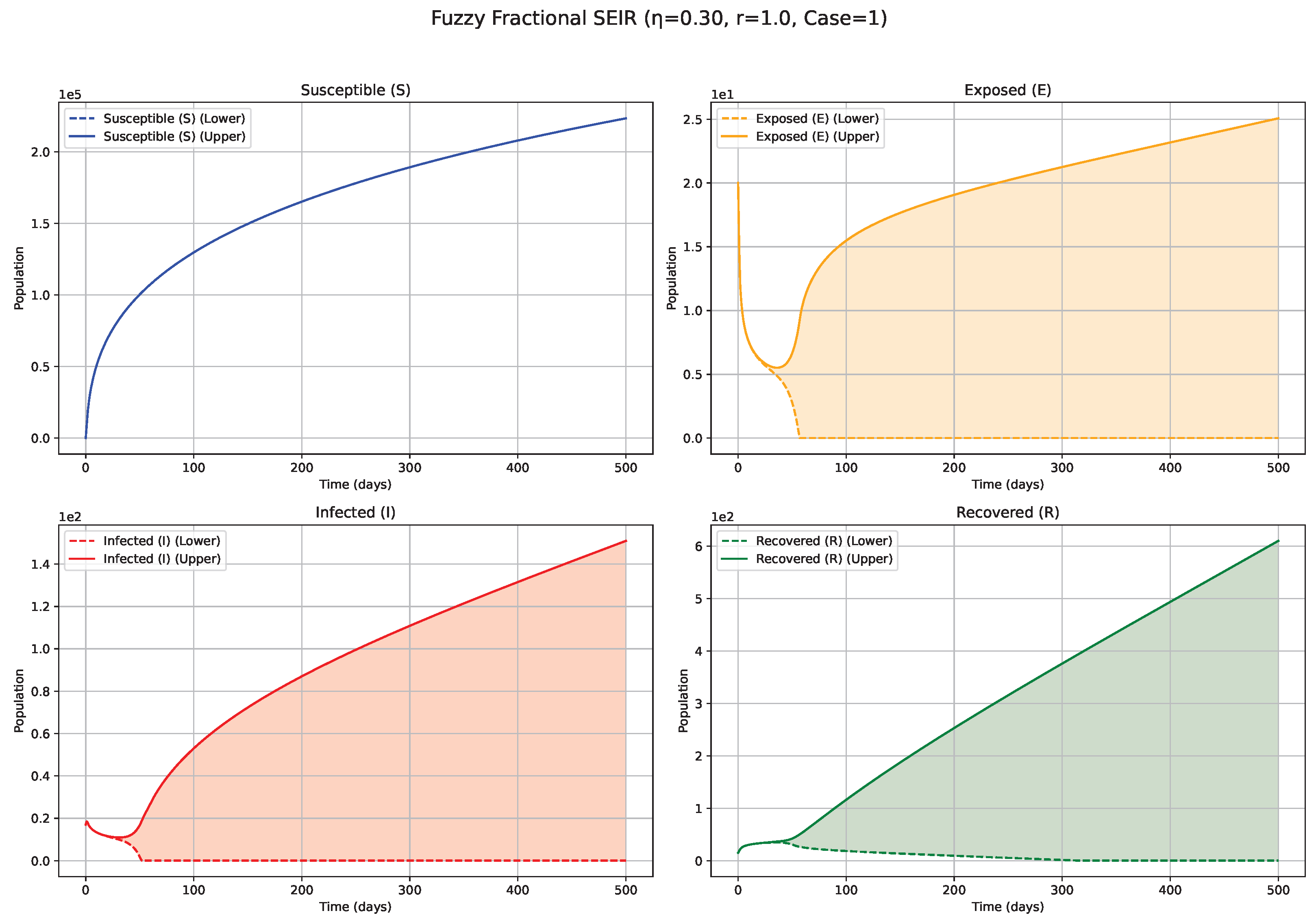
Figure 1.
Fuzzy solutions of susceptible, Exposed, Infected, and Recovered classes in case (i)-gH with order .
Figure 1.
Fuzzy solutions of susceptible, Exposed, Infected, and Recovered classes in case (i)-gH with order .
Figure 2.
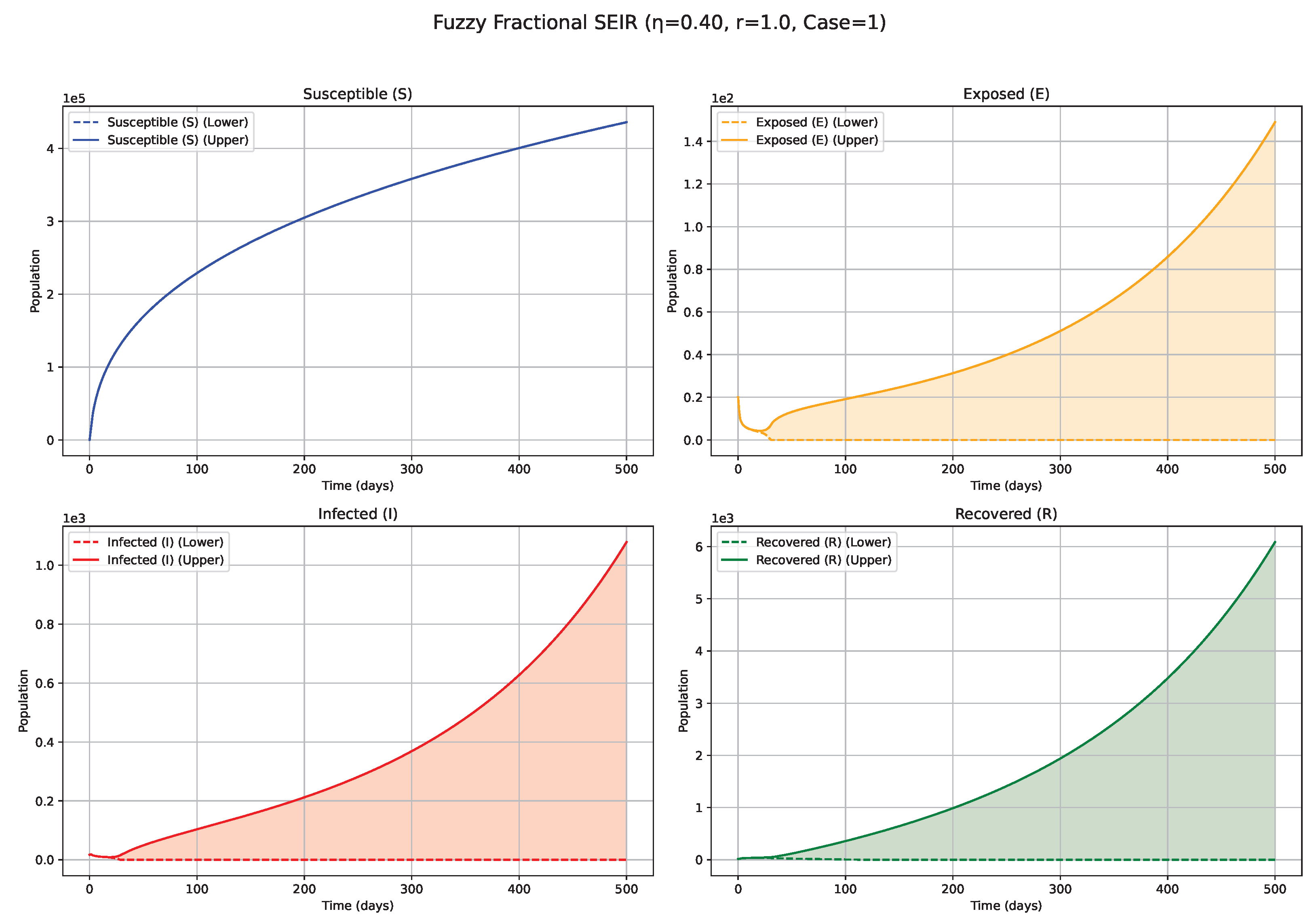
Fuzzy solutions of susceptible, Exposed, Infected, and Recovered classes in case (i)-gH with order .
Figure 2.
Fuzzy solutions of susceptible, Exposed, Infected, and Recovered classes in case (i)-gH with order .
Figure 3.
Fuzzy solutions of susceptible, Exposed, Infected, and Recovered classes in case (i)-gH with order .
Figure 3.
Fuzzy solutions of susceptible, Exposed, Infected, and Recovered classes in case (i)-gH with order .
Figure 4.
Fuzzy solutions of susceptible, Exposed, Infected, and Recovered classes in case (i)-gH with order .
Figure 4.
Fuzzy solutions of susceptible, Exposed, Infected, and Recovered classes in case (i)-gH with order .
Figure 5.
Fuzzy solutions of susceptible, Exposed, Infected, and Recovered classes in case (i)-gH with order .
Figure 5.
Fuzzy solutions of susceptible, Exposed, Infected, and Recovered classes in case (i)-gH with order .
Figure 6.
Fuzzy solutions of susceptible, Exposed, Infected, and Recovered classes in case (i)-gH with order .
Figure 6.
Fuzzy solutions of susceptible, Exposed, Infected, and Recovered classes in case (i)-gH with order .
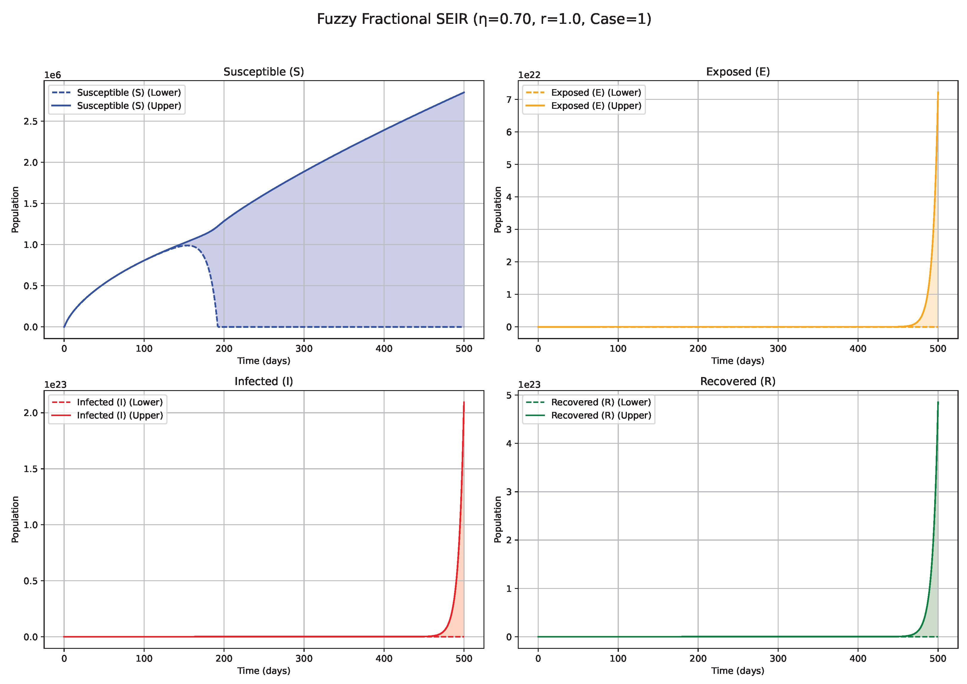
Figure 7.
Fuzzy solutions of susceptible, Exposed, Infected, and Recovered classes in case (i)-gH with order .
Figure 7.
Fuzzy solutions of susceptible, Exposed, Infected, and Recovered classes in case (i)-gH with order .
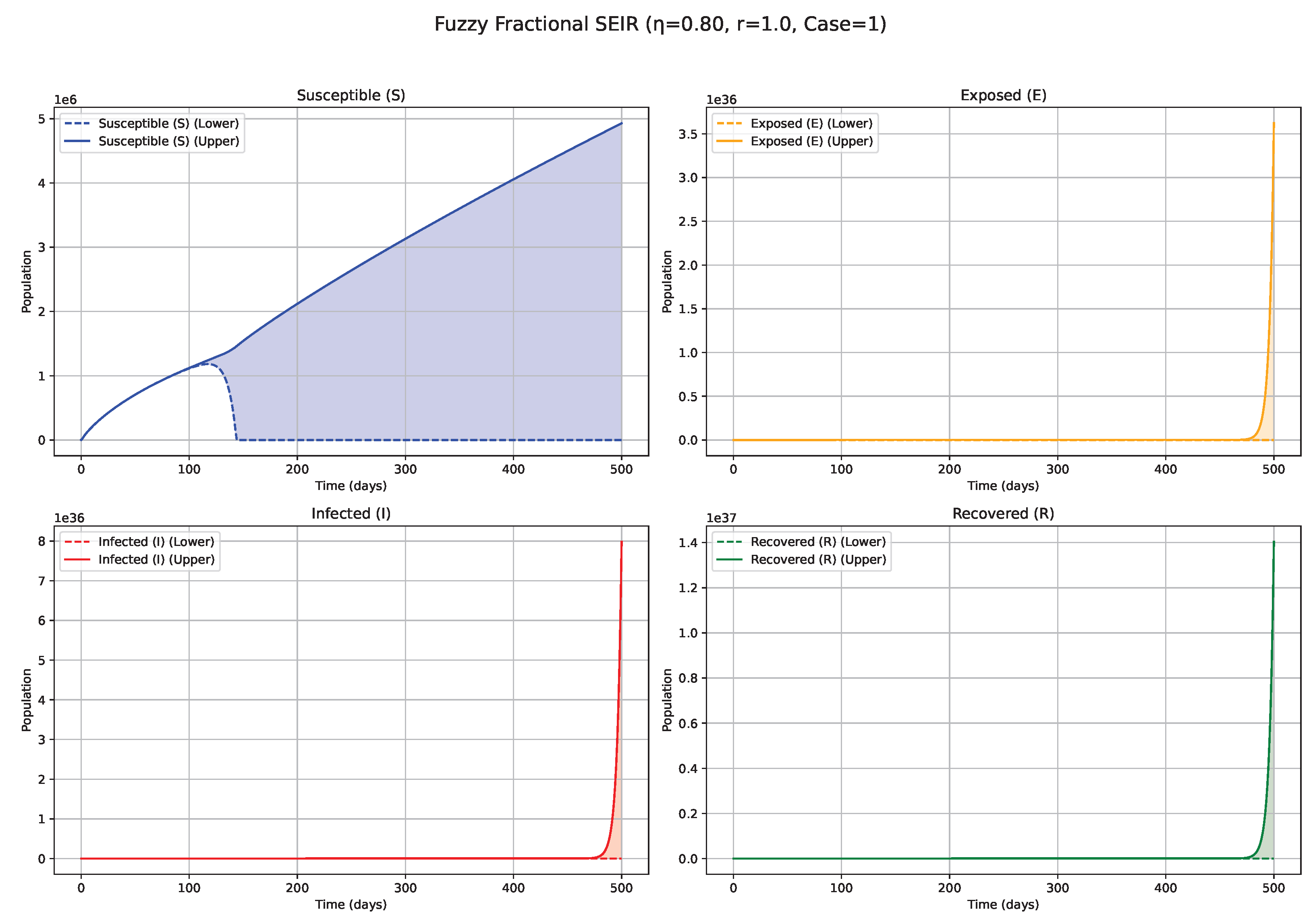
Figure 8.
Fuzzy solutions of susceptible, Exposed, Infected, and Recovered classes in case (ii)-gH with order .
Figure 8.
Fuzzy solutions of susceptible, Exposed, Infected, and Recovered classes in case (ii)-gH with order .
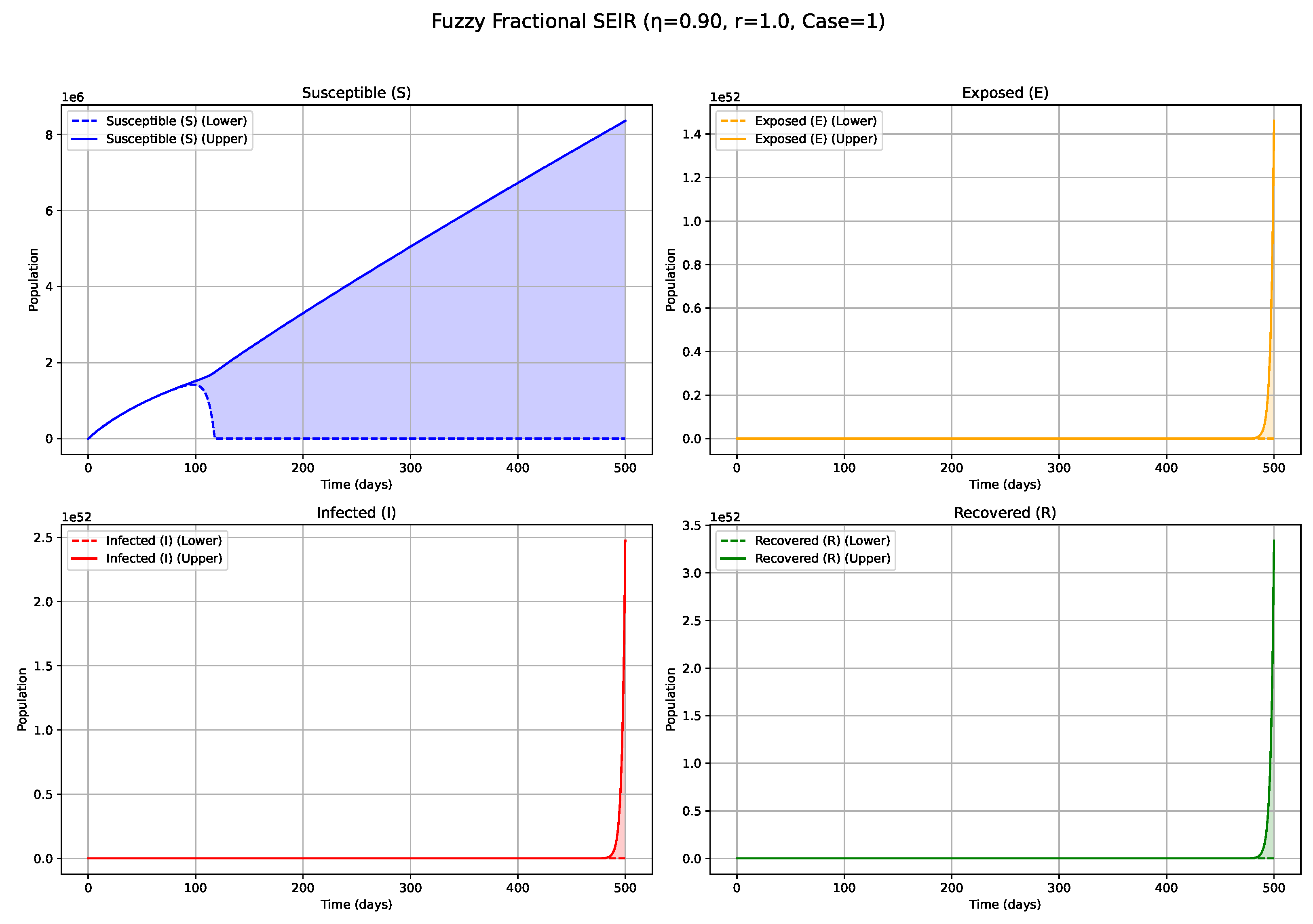
Figure 9.
Fuzzy solutions of susceptible, Exposed, Infected, and Recovered classes in case (ii)-gH with order .
Figure 9.
Fuzzy solutions of susceptible, Exposed, Infected, and Recovered classes in case (ii)-gH with order .
Figure 10.
Fuzzy solutions of susceptible, Exposed, Infected, and Recovered classes in case (ii)-gH with order .
Figure 10.
Fuzzy solutions of susceptible, Exposed, Infected, and Recovered classes in case (ii)-gH with order .
Figure 11.
Fuzzy solutions of susceptible, Exposed, Infected, and Recovered classes in case (ii)-gH with order .
Figure 11.
Fuzzy solutions of susceptible, Exposed, Infected, and Recovered classes in case (ii)-gH with order .
7. Biological Significance and Interpretation of Figures
The numerical simulations, visualized in
Figure 1,
Figure 2,
Figure 3,
Figure 4,
Figure 5,
Figure 6,
Figure 7,
Figure 8,
Figure 9,
Figure 10 and
Figure 11, demonstrate the temporal propagation of uncertainty, quantified by the width of the fuzzy bands encompassing the state variable trajectories. Furthermore, these figures elucidate the significant influence of both the fractional order (
) and the choice of generalized Hukuhara (gH) differentiability (Case 1:
vs. Case 2:
) on the resultant epidemic dynamics. Impact of Fractional Order (
)—Case 1 (
Differentiability;
Figure 1,
Figure 2,
Figure 3,
Figure 4,
Figure 5,
Figure 6 and
Figure 7,
Table 4): The fractional order
serves as an index of system memory, modulating the extent to which past states influence future epidemic progression. Low
values (e.g., 0.3, 0.4;
Figure 1 and
Figure 2): Diminishing values of
signify heightened memory effects, wherein the system’s past states exert a more substantial influence on current and future dynamics. Biologically, such scenarios may reflect the impact of factors like prolonged immunity, persistent environmental viral reservoirs (e.g., the virus surviving for a time on surfaces or in contaminated water sources), or slowly evolving public health behaviors. Consequently, the simulated epidemic curves for Exposed (
E) and Infected (
I) compartments display attenuated, wider peaks, characteristic of a protracted epidemic wave and a more pronounced “flattening of the curve.” The associated fuzzy bands, representing uncertainty, also tend to remain wider for extended periods, indicating sustained uncertainty under strong memory conditions. Medium
values (e.g., 0.5, 0.6, 0.7;
Figure 3,
Figure 4 and
Figure 5): Intermediate
values represent a transitional regime with moderate memory effects. The epidemic wave becomes more distinctly defined compared with low
scenarios, featuring earlier and comparatively sharper peaks, indicating a tempered influence of historical system states on the epidemiological trajectory. High
values (e.g., 0.8, 0.9, approaching 1;
Figure 6 and
Figure 7): Conversely, higher
values lead to system dynamics that increasingly resemble those of classical integer-order models, characterized by diminished memory effects. Epidemics under these conditions progress more rapidly, exhibit sharper and higher incidence peaks, and resolve more quickly, reflecting a greater responsiveness to contemporaneous conditions. The fuzzy uncertainty bands may also converge more rapidly as the system’s trajectory becomes more deterministic.
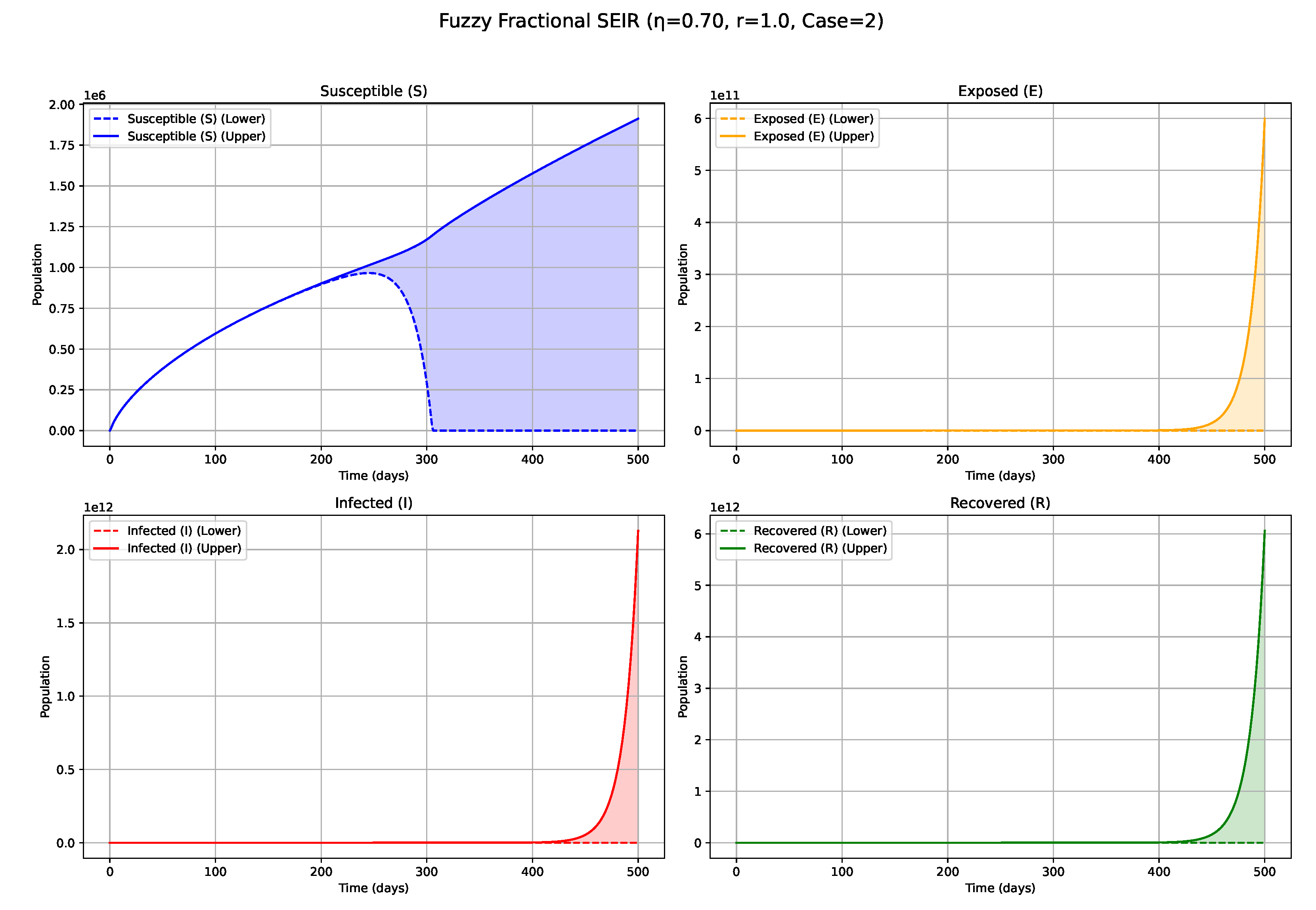
Impact of Derivative Type—Case 2 (
Differentiability;
Figure 8,
Figure 9,
Figure 10 and
Figure 11,
Table 5): The selection of gH-differentiability profoundly alters the interpretation of the fuzzy system’s evolution, particularly for the Exposed (
E) and Infected (
I) compartments. Low
values (e.g., 0.3;
Figure 8): Under
differentiability, particularly at low
values, the system demonstrates pronounced memory retention and sluggish dynamics. Notably, for the E and I compartments, instead of a distinct outbreak peak as observed in Case 1, a slow, monotonic decline from initial fuzzy values is observed. This suggests a dynamic dominated by disease fade-out or a very gradual transition towards an equilibrium state, without the emergence of a significant new infection wave. The historical states heavily influence this slow decay, with new infection generation being insufficient to trigger a resurgence within the simulation period. Higher
values (e.g., 0.7, 0.9;
Figure 10 and
Figure 11): As
increases within Case 2, the rate of this decay or stabilization accelerates. However, the fundamental characteristic of not producing a new prominent outbreak peak (for
E and
I compartments, unlike in Case 1) persists. The system continues to reflect a decay or stabilization trajectory, though with a progressively weaker influence of past states compared with lower
values in this differentiability case. The contrasting dynamics between Case 1 and Case 2 underscore the nuanced complexities introduced by the fuzzy fractional framework. Case 1 (
) dynamics are generally consistent with the canonical pattern of active epidemic propagation followed by decline. In contrast, Case 2 (
) dynamics, especially for the
E and
I compartments may represent scenarios where initial conditions or parameterizations favor direct decay or slow convergence towards an equilibrium. This behavior could be attributed to the specific mathematical properties of
differentiability when applied to the model’s governing equations and the way it interacts with the fuzzy representation of state variables. This distinction is of paramount importance for epidemiological modeling, as the choice of
-differentiability can lead to qualitatively disparate predictions regarding the emergence and characteristics of future epidemic waves.
From a public health perspective, the interval-valued solutions generated by this fuzzy fractional framework offer significant advantages for decision-making under uncertainty. Instead of providing a single, deterministic prediction for the epidemic’s peak or duration, the model provides a range of possibilities encapsulated within the fuzzy bands. This allows authorities to engage in more robust planning. For example, the upper bound of the infected compartment’s trajectory can inform worst-case scenario planning for hospital bed capacity, while the lower bound can help establish a baseline for resource allocation. The width of the fuzzy band itself is a quantitative measure of predictive uncertainty. A wider band might prompt decision-makers to adopt more flexible, adaptive strategies or to invest in better data collection to reduce uncertainty. Thus, these fuzzy results can be used to formulate more resilient public health policies for vaccination campaigns, resource stockpiling, and risk communication that account for the inherent unpredictability of epidemic dynamics.
8. Conclusions
In this work, we have developed and analyzed an SEIR influenza epidemic model incorporating fuzzy Atangana–Baleanu–Caputo (ABC) fractional derivatives and a Crowley–Martin incidence rate. This approach uniquely combines the ability to represent inherent uncertainties in epidemiological parameters and state variables (through fuzzy numbers) with the capacity to model memory effects and non-local dynamics (through fractional calculus). The Crowley–Martin incidence rate is included to provide a more flexible mechanism that can potentially enhance realism by accounting for saturation effects at high densities of susceptible or infectious individuals. The SEIR model with Crowley–Martin incidence and ABC fractional derivatives provides a flexible framework for studying disease dynamics. Key properties, such as positivity and boundedness, ensure biological relevance. The basic reproduction number acts as a threshold: the DFE is locally stable if and unstable if . An endemic equilibrium may exist and be stable if . The fractional order and the fuzzy nature of the derivatives/parameters add significant complexity to the analysis, requiring specialized mathematical tools, but offer the potential for a more realistic description of real-world epidemic processes with memory and uncertainty. Numerical simulations are often essential to explore the dynamics of such complex models. This work provides a more nuanced understanding by simultaneously accounting for memory effects and inherent uncertainties. The numerical simulations demonstrate the profound impact of the fractional order and the type of fuzzy differentiability on epidemic trajectories, yielding interval-valued predictions that are more informative for public health decision-making than single-point estimates. This framework lays the groundwork for more sophisticated and realistic epidemiological models that can better capture the complexities of infectious disease spread. However, we acknowledge that the practical validation of this model is a critical next step. Future work should focus on applying this framework to a real-world case study using influenza surveillance data. Such an investigation would involve the complex task of estimating the fuzzy parameters from empirical data and validating the model’s interval-valued predictions against observed epidemic trajectories. This would bridge the gap between this theoretical development and its potential application in public health planning and decision-making under uncertainty, thereby demonstrating its full practical utility.
It is important to acknowledge the limitations of the current model, which define avenues for future research. First, our model assumes homogeneous mixing within the population, a common simplification that does not account for spatial or social structures. Second, the analysis relies on parameters from the literature rather than fitting them to a specific epidemiological dataset, a task that would require advanced statistical methods for fuzzy fractional systems. Third, while the ABC fractional derivative provides a sophisticated memory kernel, its specific form may not be optimal for all biological processes. Finally, the complexity of the fuzzy fractional framework itself can be a barrier to direct implementation by public health agencies. These limitations underscore that our model serves as a foundational step, demonstrating the potential of this approach, rather than a final, universally applicable predictive tool.


 ,
, 
