Dynamic Analysis of a Fractional Breast Cancer Model with Incommensurate Orders and Optimal Control

Abstract

This paper constructs a fundamental mathematical model to depict the therapeutic effects of two drugs on breast cancer patients. The model is described by fractional order differential equations with two control variables. Two scenarios are considered: the constant control and the optimal control. For the constant control scenario, the existence and uniqueness of the solution of the system are proved by using the fixed point theorem and combining with the Caputo–Fabrizio fractional derivative; then, the sufficient conditions for the existence and stability of the system’s equilibriums are derived. For the optimal control scenario, the optimal control solution is obtained by using the Pontryagin’s maximum principle. To further validate the effectiveness of the theoretical results, numerical simulations were conducted. The results show that the parameters have significant sensitivity to the dynamic behavior of the system.

1. Introduction

Breast cancer, as one of the most common malignant tumors among women globally, seriously threatens women’s health and lives. In recent years, with the change in lifestyle, the acceleration of the aging process of the population, and the influence of environmental factors, the incidence rate of breast cancer has shown a continuous upward trend [1]. According to the global cancer data released in 2020 by the International Agency for Research on Cancer (IARC) of the World Health Organization (WHO), the number of new breast cancer cases exceeded 2.26 million. For the first time, it surpassed lung cancer and became the most common cancer globally [2]. In our country, breast cancer is also the malignant tumor with the highest incidence rate among women, and the age of onset shows a trend of becoming younger. The incidence rate in urban areas is significantly higher than that in rural areas [3].

Breast cancer is a malignant tumor that originates from breast cells. Its pathological changes usually begin in the inner epithelial layer of the milk ducts or in the lobules responsible for milk production. Different from benign tumors, malignant tumors such as breast cancer have the ability to metastasize to other areas of the body [4]. In the early stage of breast cancer, patients usually develop painless small lumps in the breast. When it progresses to the advanced stage, the breast skin may show an orange peel-like change, and the nipple may secrete bloody fluid. Currently, there are various treatment methods for breast cancer, including chemotherapy, hormone therapy, radiotherapy, surgery, and targeted therapy [5,6,7,8,9]. These cancer treatment methods aim to induce apoptosis in cancer tissues, eliminate malignant tissues, or block the transmission of cell division signals to the tumor [10]. Each technique has achieved some degree of success in shrinking or eliminating tumors, but cancer treatment remains one of the most challenging problems in the field of modern medicine.

Epidemiology, as an important branch of medicine, focuses on exploring the causes of diseases and explaining the patterns and mechanisms by which diseases affect different populations. Its related data play a crucial role in evaluating and screening preventive measures and managing individuals with diseases. In the academic literature, most diseases are associated with corresponding epidemiological mathematical models, and these models are continuously updated to more accurately capture the dynamic changes in diseases. They are of great practical value for understanding the development trend of diseases, predicting the future direction of diseases, and formulating appropriate preventive strategies. In [11], Mufudza simulated the body’s natural response to tumor growth by incorporating immune cell populations to study the impact of excessive estrogen on the dynamics of breast cancer. In [12], a tumor-immune model with time delay is introduced, and the model focused on studying the growth and survival of tumor cells under the surveillance of the immune system.

The authors in [13] proposed a series of classical tumor growth models, including the linear model and the exponential model. These models are of great significance for the biological theory of tumor growth and the application of mathematical models in the research of anti-cancer drugs. The authors in [14] proposed a nonlinear mathematical model of cancer immunosurveillance that considered intra-tumor heterogeneity and cell-mediated immune responses. The model described in vivo phenomena such as tumor dormancy and immunoediting, revealed types of tumor attractors through bifurcation analysis, and simulated tumor elimination and escape scenarios using a stochastic model. The authors in [15] proposed an optimal control model for the interaction between tumors and the immune system under chemotherapy. They constructed the objective functions with both linear control and quadratic control. The results of numerical simulation show that under these two control strategies, the objective functions can effectively reduce the number of tumor cells. Reference [16] proposed a fractional-order tumor growth model with (or without) a singular kernel and explored the optimal treatment plan for cancer.

Compared with integer order calculus, fractional calculus provides a brand-new perspective for describing the complex dynamic characteristics of real-world systems with memory effects. It can more accurately characterize complex phenomena and offers stronger modeling flexibility. At present, this approach has been widely applied in various fields, such as physics [17], chemistry [18], financial science [19], and engineering [20]. In [21], the dynamics of the fractional-order model of tumor growth was studied. The results showed that fractional derivatives have significant advantages, as they can be flexibly adjusted to achieve the best fitness to the real information. The authors explored the use of diffusion-weighted imaging technology based on fractional-order model to distinguish benign and malignant breast lesions in [22]. The authors of [23] applied the Atangana–Baleanu–Caputo fractional order derivative to conduct optimal control research on the mathematical model of cancer treatment. The authors of [24] used neural networks to carry out numerical analysis on the immuno-chemotherapy treatment scheme for breast cancer based on the fractional-order mathematical model.

In addition to the mathematical interpretation of tumor growth mechanisms, formulating appropriate treatment strategies has always been a crucial issue. In this regard, control design strategies can be used to optimize drug dosages, contributing to the improvement of treatment outcomes. For example, in the research on the transmission mechanism of HIV (human immunodeficiency virus) [25,26,27], as well as the pathological analysis and exploration of treatment strategies for breast cancer [28,29].

The Caputo–Fabrizio derivative has a more flexible ability to characterize memory properties. With its unique kernel function form, it can more precisely adapt to the influences generated by different types of information when describing complex memory effects, showing significant advantages compared with other forms of derivatives [30].

The authors constructed a five-dimensional ordinary differential model to depict the interrelationships among cancer stem cells, tumor cells, healthy cells, immune cells, and estrogen in [31]. Based on this model, Ref. [32] further explored the dynamic behaviors of various types of cells in the context of fractional order. Inspired by Refs. [32,33], the model is modified as follows:

$$\left\{\begin{array}{ccc}{}_0{}^{C}D_t^{{\alpha }_1}C(t)\hfill & =\hfill & {\displaystyle k_{1}C\left(t\right)\left(1-\frac{C\left(t\right)}{M_1}\right)-{\gamma }_{1}I\left(t\right)C\left(t\right)+\frac{p_{1}C\left(t\right)E\left(t\right)}{a_1+C\left(t\right)},}\hfill \\ {}_0{}^{C}D_t^{{\alpha }_2}T(t)\hfill & =\hfill & {\displaystyle k_{2}C\left(t\right)\frac{C\left(t\right)}{M_1}\left(1-\frac{T\left(t\right)}{M_2}\right)-n_{1}T\left(t\right)-{\gamma }_{2}I\left(t\right)T\left(t\right)+\frac{p_{2}T\left(t\right)E\left(t\right)}{a_2+T\left(t\right)}-u_1\left(t\right)T\left(t\right),}\hfill \\ {}_0{}^{C}D_t^{{\alpha }_3}H(t)\hfill & =\hfill & {\displaystyle qH\left(t\right)\left(1-\frac{H\left(t\right)}{M_3}\right)-\delta H\left(t\right)T\left(t\right)-\frac{p_{3}H\left(t\right)E\left(t\right)}{a_3+H\left(t\right)},}\hfill \\ {}_0{}^{C}D_t^{{\alpha }_4}I(t)\hfill & =\hfill & {\displaystyle \varsigma +\frac{\rho I\left(t\right)T\left(t\right)}{\omega +T\left(t\right)}-{\gamma }_{3}I\left(t\right)T\left(t\right)-n_{2}I\left(t\right)-\frac{\beta I\left(t\right)E\left(t\right)}{\nu +E\left(t\right)},}\hfill \\ {}_0{}^{C}D_t^{{\alpha }_5}E(t)\hfill & =\hfill & {\displaystyle \iota -\left(\epsilon +u_2\left(t\right)+\frac{d_{1}C\left(t\right)}{a_1+C\left(t\right)}+\frac{d_{2}T\left(t\right)}{a_2+T\left(t\right)}+\frac{d_{3}H\left(t\right)}{a_3+H\left(t\right)}\right)E\left(t\right),}\hfill \end{array}\right.$$

(1)

with initial conditions

$$C_0\left(t\right)=C\left(0\right),T_0\left(t\right)=T\left(0\right),H_0\left(t\right)=H\left(0\right),I_0\left(t\right)=I\left(0\right),E_0\left(t\right)=E\left(0\right),$$

where ${}_0{}^{C}D_t^{{\alpha }_n}$ is the Caputo fractional order derivative for $n=1,2,3,4,5$ and ${\alpha }_n\in (0,1]$. Here, $C\left(t\right),T\left(t\right),H\left(t\right),I\left(t\right),$ and $E\left(t\right)$ represent the densities of cancer stem cells, tumor cells, healthy cells, immune cells, and excessive estrogen at time t, respectively. $u_1\left(t\right),u_2\left(t\right)$ represent the efficacy of Trastuzumab and Aromatase Inhibitors drugs.

It can be clearly observed that there are obvious differences in the setting of the time dimensions on the left and right sides of system (1). To ensure consistency in time dimension, we adopt the method proposed in [34]. The specific content of the optimized model is as follows:

$$\left\{\begin{array}{ccc}{\displaystyle \frac{1}{{\sigma }^{1-{\alpha }_1}}}{}_0{}^{C}D_t^{{\alpha }_1}C(t)\hfill & =\hfill & {\displaystyle k_{1}C\left(t\right)\left(1-\frac{C\left(t\right)}{M_1}\right)-{\gamma }_{1}I\left(t\right)C\left(t\right)+\frac{p_{1}C\left(t\right)E\left(t\right)}{a_1+C\left(t\right)},}\hfill \\ {\displaystyle \frac{1}{{\sigma }^{1-{\alpha }_2}}}{}_0{}^{C}D_t^{{\alpha }_2}T(t)\hfill & =\hfill & {\displaystyle k_{2}C\left(t\right)\frac{C\left(t\right)}{M_1}\left(1-\frac{T\left(t\right)}{M_2}\right)-n_{1}T\left(t\right)-{\gamma }_{2}I\left(t\right)T\left(t\right)+\frac{p_{2}T\left(t\right)E\left(t\right)}{a_2+T\left(t\right)}-u_1\left(t\right)T\left(t\right),}\hfill \\ {\displaystyle \frac{1}{{\sigma }^{1-{\alpha }_3}}}{}_0{}^{C}D_t^{{\alpha }_3}H(t)\hfill & =\hfill & {\displaystyle qH\left(t\right)\left(1-\frac{H\left(t\right)}{M_3}\right)-\delta H\left(t\right)T\left(t\right)-\frac{p_{3}H\left(t\right)E\left(t\right)}{a_3+H\left(t\right)},}\hfill \\ {\displaystyle \frac{1}{{\sigma }^{1-{\alpha }_4}}}{}_0{}^{C}D_t^{{\alpha }_4}I(t)\hfill & =\hfill & {\displaystyle \varsigma +\frac{\rho I\left(t\right)T\left(t\right)}{\omega +T\left(t\right)}-{\gamma }_{3}I\left(t\right)T\left(t\right)-n_{2}I\left(t\right)-\frac{\beta I\left(t\right)E\left(t\right)}{\nu +E\left(t\right)},}\hfill \\ {\displaystyle \frac{1}{{\sigma }^{1-{\alpha }_5}}}{}_0{}^{C}D_t^{{\alpha }_5}E(t)\hfill & =\hfill & {\displaystyle \iota -\left(\epsilon +u_2\left(t\right)+\frac{d_{1}C\left(t\right)}{a_1+C\left(t\right)}+\frac{d_{2}T\left(t\right)}{a_2+T\left(t\right)}+\frac{d_{3}H\left(t\right)}{a_3+H\left(t\right)}\right)E\left(t\right).}\hfill \end{array}\right.$$

(2)

The biological meanings of all parameters are presented in

Table 1. The biological meanings for the variables and parameters in system (2).

$\mathbf{Variables}$	$\mathbf{Description}$
$C\left(t\right)$	the density of cancer stem cells
$T\left(t\right)$	the density of tumor cells
$H\left(t\right)$	the density of healthy cells
$I\left(t\right)$	the density of immune cells
$E\left(t\right)$	the density of excess estrogen
$\mathbf{Parameters}$	$\mathbf{Description}$	$\mathbf{Values}$	$\mathbf{Refs}$
$k_1$	the normal rate of division for cancer stem cells	[0.10, 0.95] day−1	[32]
$k_2$	the normal rate of division for tumor cells	0.514 day−1	[32]
q	the normal rate of division for healthy cells	0.70 day−1	[33]
$M_1$	the carrying capacity of cancer stem cells	$2.27\times {10}^6$ cells	[32]
$M_2$	the carrying capacity of tumor cells	$2.27\times {10}^7$ cells	[33]
$M_3$	the carrying capacity of healthy cells	$2.5\times {10}^6$ cells	[33]
${\gamma }_1$	the death rate of cancer stem cells	$3\times {10}^{-7}$${\displaystyle \frac{1}{\left(\mathrm{cell}\right)\left(\mathrm{day}\right)}}$	[33]
${\gamma }_2$	the death rate of tumor cells due to immune	$3\times {10}^{-6}$${\displaystyle \frac{1}{\left(\mathrm{cell}\right)\left(\mathrm{day}\right)}}$	[33]
	cells’ response
${\gamma }_3$	the death rate of immune cells due to tumor	$1\times {10}^{-7}$${\displaystyle \frac{1}{\left(\mathrm{cell}\right)\left(\mathrm{day}\right)}}$	[33]
	cells’ response
$p_1$	represent the rate at which estrogen helps to	600 ${\displaystyle \frac{\mathrm{cell}}{\left(\mathrm{day}\right)(\mathrm{pg}/\mathrm{mL})}}$	[33]
	proliferate cancer stem cells
$p_2$	represent the rate at which estrogen helps to	[0, 600] ${\displaystyle \frac{\mathrm{cell}}{\left(\mathrm{day}\right)(\mathrm{pg}/\mathrm{mL})}}$	[32,33]
	proliferate tumor cells
$p_3$	the rate at which healthy cells are lost to DNA	100 ${\displaystyle \frac{\mathrm{cell}}{\left(\mathrm{day}\right)(\mathrm{pg}/\mathrm{mL})}}$	[33]
	mutation by estrogen presence
$a_1$	the number of cancer stem cells at which the rate	$1.135\times {10}^6$ cells	[33]
	of absorption is at half its maximum
$a_2$	the number of tumor cells at which the rate of	$1.135\times {10}^7$ cells	[33]
	absorption is at half its maximum
$a_3$	the number of healthy cells at which the rate of	$1.25\times {10}^7$ cells	[33]
	absorption is at half its maximum
$n_1$	the normal death rate of tumor cells	0.01 day−1	[33]
$n_2$	the normal death rate of immune cells	0.29 day−1	[33]
$\delta$	the death rate of healthy cells due to competition	$6\times {10}^{-8}$${\displaystyle \frac{1}{\left(\mathrm{cell}\right)\left(\mathrm{day}\right)}}$	[33]
	with tumor cells
$\varsigma$	the source rate of immune cells	$1.3\times {10}^4$${\displaystyle \frac{\mathrm{cell}}{\mathrm{day}}}$	[32]
$\rho$	the immune cells’ response rate	0.20 ${\displaystyle \frac{1}{\mathrm{day}}}$	[33]
$\omega$	the immune cells threshold	$3\times {10}^5$ cells	[32]
$\beta$	the rate of immune suppression by estrogen	0.20 ${\displaystyle \frac{1}{\mathrm{day}}}$	[33]
$\nu$	the estrogen threshold	400 ${\displaystyle \frac{\mathrm{pgm}}{\mathrm{L}}}$	[33]
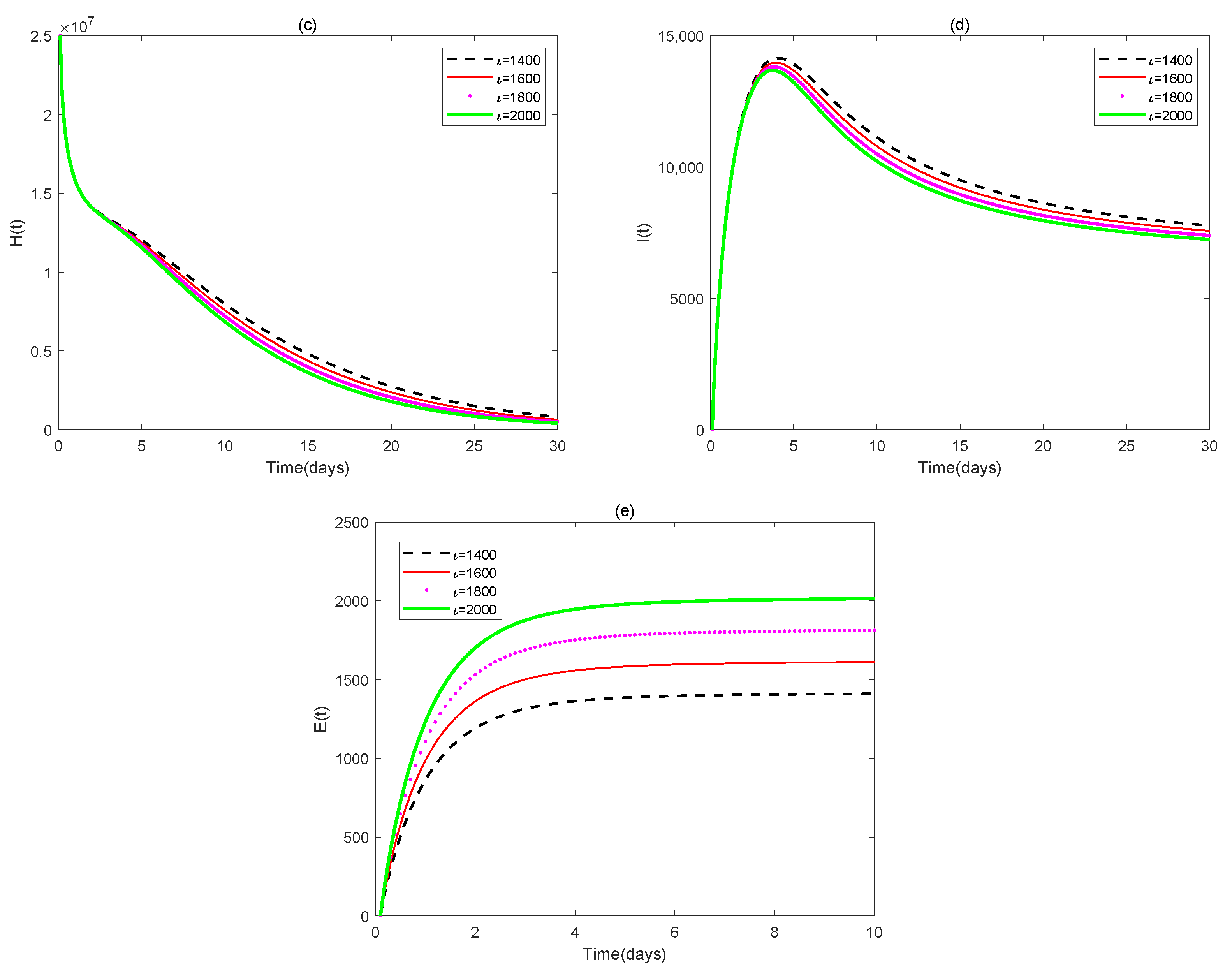
$\iota$	the continuous infusion of estrogen	[1400, 2000] ${\displaystyle \frac{\mathrm{pgm}}{\mathrm{day}\mathrm{L}}}$	[32,33]
$\epsilon$	the washout rate of estrogen by the body	0.97 day−1	[33]
$d_1$	the absorption rate of estrogen by cancer stem cells	0.01 day−1	[33]
$d_2$	the absorption rate of estrogen by tumor cells	0.01 day−1	[33]
$d_3$	the absorption rate of estrogen by healthy cells	0.01 day−1	[33]
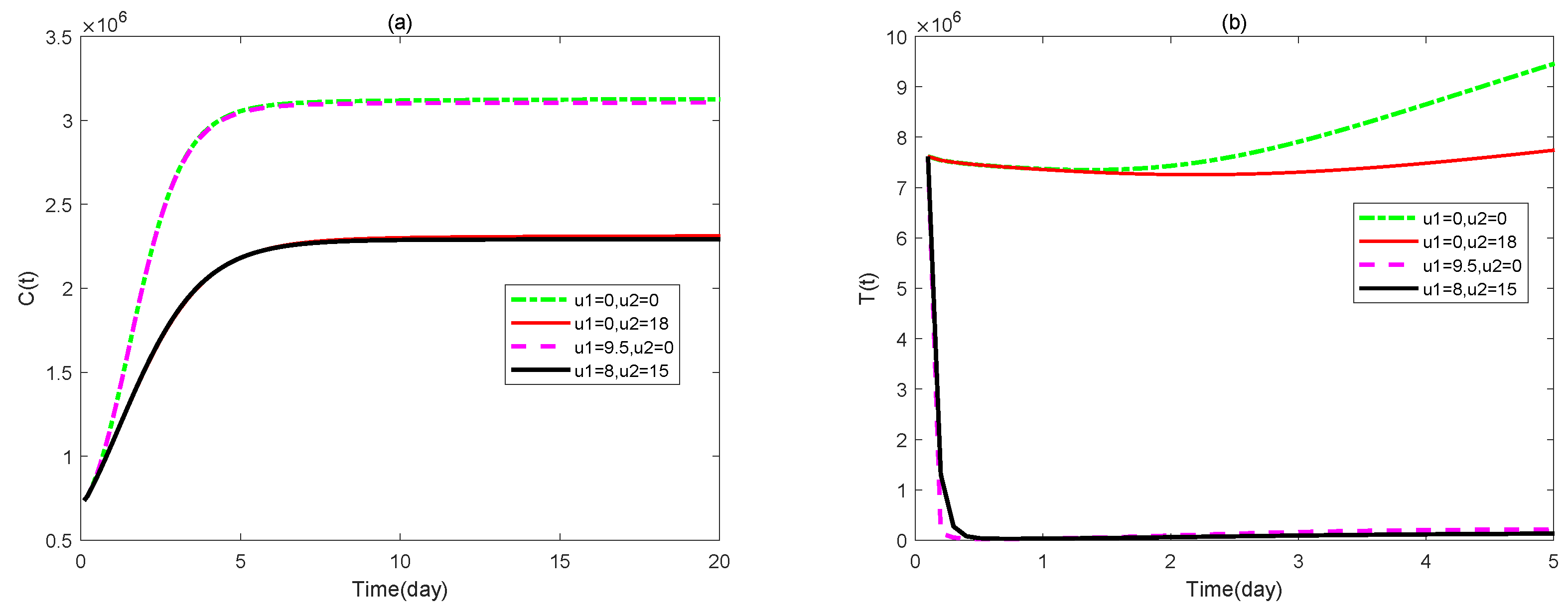
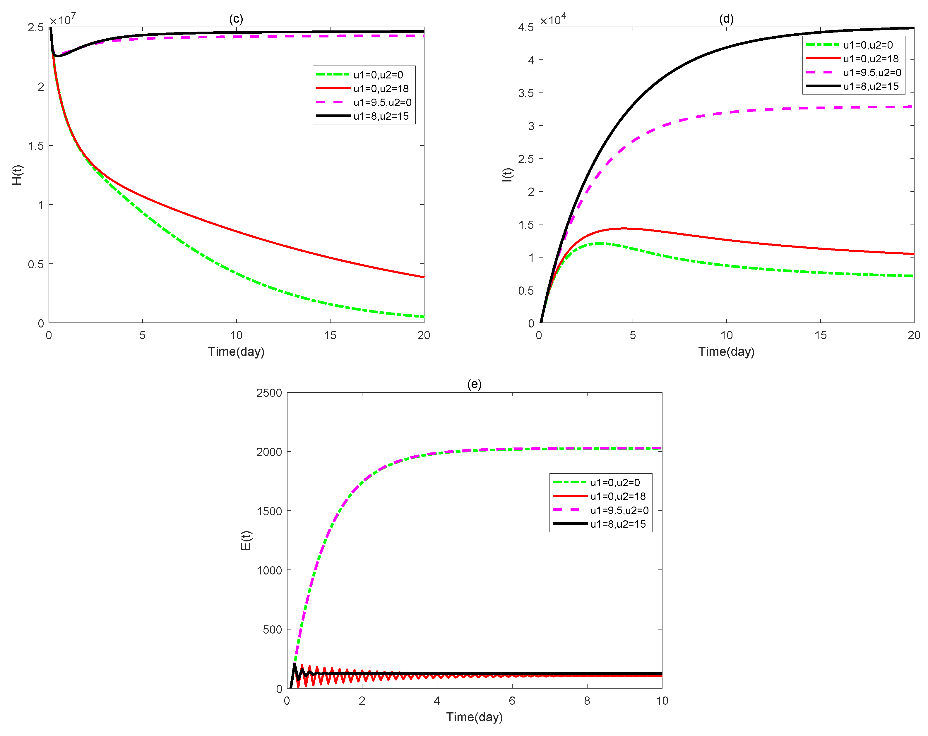
$u_1$	represent the efficacy of Trastuzumab	$--$	$--$
$u_2$	represent the efficacy of Aromatase Inhibitors	$--$	$--$

.

Compared with the exploration of the therapeutic effects of three drugs on breast cancer patients from a clinical medicine perspective in [33] and the simple focus on the breast cancer model in [32], this paper focuses on the study of the combined treatment of breast cancer with two drugs (Trastuzumab and Aromatase Inhibitors). Through numerical simulations under multiple scenarios such as constant control and optimal control of the constructed mathematical model, the research conclusions are verified from a mathematical level.

The structure of this paper is arranged as follows: In Section 2, we will prove the existence and uniqueness of the solution to system (2) and explore the existence and stability of the equilibriums of system (2). In Section 3, we conduct an in-depth study of the mathematical model of breast cancer with an optimal control strategy. In Section 4, some numerical simulations are carried out. In the last section, this paper summarizes and discusses the research work, looks forward to future research directions, and provides references for the development of related fields.

2. Qualitative Analysis of the System

In this section, we will analyze the existence and uniqueness of solutions of system (2). Before that, we will first review some lemmas.

Lemma 1

([35]). For an integrable function $f\left(t\right)$, the Caputo–Fabrizio (CF) fractional derivative without a singular kernel in Liouville–Caputo sense is given by

$$\begin{array}{c}\hfill \begin{array}{c}\hfill {}_0{}^{CF}D_t^{\alpha }f(t)={\displaystyle \frac{M\left(\alpha \right)}{n-\alpha }}{\int }_0^t{\displaystyle \frac{d^n}{d{t}^n}}f\left(\theta \right)exp\left[-{\displaystyle \frac{\alpha }{n-\alpha }}(t-\theta )\right]\mathrm{d}\theta ,n-1<\alpha \le n,\end{array}\end{array}$$

(3)

where $M\left(\alpha \right)$ is a normalization function such that $M\left(0\right)=M\left(1\right)=1$.

The Laplace transform of the fractional derivative of CF is given as follows:

$$\begin{array}{c}\hfill \begin{array}{c}\hfill \pounds \{{}_0{}^{CF}D_t^{\alpha }f(t)\}(\tau )={\displaystyle \frac{\tau F\left(\tau \right)-f\left(0\right)}{\tau +\alpha (1-\tau )}}.\end{array}\end{array}$$

(4)

Lemma 2

([36]). The fractional integral of order α $(0<\alpha \le 1)$ of function $f\left(t\right)$ is defined below

$$\begin{array}{c}\hfill \begin{array}{c}\hfill {}_0{}^{CF}I_t^{\alpha }f(t)={\displaystyle \frac{2(1-\alpha )}{(2-\alpha )M\left(\alpha \right)}}f\left(t\right)+{\displaystyle \frac{2\alpha }{(2-\alpha )M\left(\alpha \right)}}{\int }_0^{t}f\left(\tau \right)\mathrm{d}\tau ,t\ge 0,\end{array}\end{array}$$

(5)

where

$$\begin{array}{c}\hfill \begin{array}{c}\hfill {\displaystyle M\left(\alpha \right)=\frac{2}{2-\alpha },0<\alpha \le 1.}\end{array}\end{array}$$

(6)

Then, system (2) in a Caputo–Fabrizio sense will become

$$\left\{\begin{array}{c}{\displaystyle {\frac{1}{{\sigma }^{1-{\alpha }_1}}}_0^{CF}{D}_t^{{\alpha }_1}C\left(t\right)=k_{1}C\left(t\right)\left(1-\frac{C\left(t\right)}{M_1}\right)-{\gamma }_{1}I\left(t\right)C\left(t\right)+\frac{p_{1}C\left(t\right)E\left(t\right)}{a_1+C\left(t\right)},}\hfill \\ {\displaystyle {\frac{1}{{\sigma }^{1-{\alpha }_2}}}_0^{CF}{D}_t^{{\alpha }_2}T\left(t\right)=k_{2}C\left(t\right)\frac{C\left(t\right)}{M_1}\left(1-\frac{T\left(t\right)}{M_2}\right)-n_{1}T\left(t\right)-{\gamma }_{2}I\left(t\right)T\left(t\right)+\frac{p_{2}T\left(t\right)E\left(t\right)}{a_2+T\left(t\right)}-u_1\left(t\right)T\left(t\right),}\hfill \\ {\displaystyle {\frac{1}{{\sigma }^{1-{\alpha }_3}}}_0^{CF}{D}_t^{{\alpha }_3}H\left(t\right)=qH\left(t\right)\left(1-\frac{H\left(t\right)}{M_3}\right)-\delta H\left(t\right)T\left(t\right)-\frac{p_{3}H\left(t\right)E\left(t\right)}{a_3+H\left(t\right)},}\hfill \\ {\displaystyle {\frac{1}{{\sigma }^{1-{\alpha }_4}}}_0^{CF}{D}_t^{{\alpha }_4}I\left(t\right)=\varsigma +\frac{\rho I\left(t\right)T\left(t\right)}{\omega +T\left(t\right)}-{\gamma }_{3}I\left(t\right)T\left(t\right)-n_{2}I\left(t\right)-\frac{\beta I\left(t\right)E\left(t\right)}{\nu +E\left(t\right)},}\hfill \\ {\displaystyle {\frac{1}{{\sigma }^{1-{\alpha }_5}}}_0^{CF}{D}_t^{{\alpha }_5}E\left(t\right)=\iota -\left(\epsilon +u_2\left(t\right)+\frac{d_{1}C\left(t\right)}{a_1+C\left(t\right)}+\frac{d_{2}T\left(t\right)}{a_2+T\left(t\right)}+\frac{d_{3}H\left(t\right)}{a_3+H\left(t\right)}\right)E\left(t\right),}\hfill \end{array}\right.$$

(7)

with initial conditions

$$C_0\left(t\right)=C\left(0\right),T_0\left(t\right)=T\left(0\right),H_0\left(t\right)=H\left(0\right),I_0\left(t\right)=I\left(0\right),E_0\left(t\right)=E\left(0\right),$$

where ${}_0{}^{CF}D_t^{{\alpha }_n}$ is the Caputo–Fabrizio fractional order derivative for $n=1,2,3,4,5$ and ${\alpha }_n\in (0,1]$.

2.1. The Existence of Solution

Next, we will conduct an in-depth exploration of the existence and uniqueness of solutions of system (7). In this process, we will use the fixed point theorem to determine the existence of solution. First, we transform model (7) into the following integral equations:

$$\left\{\begin{array}{c}{\displaystyle C\left(t\right)-C\left(0\right)={}_0{}^{CF}I_t^{{\alpha }_1}\left[k_{1}C\left(t\right)\left(1-\frac{C\left(t\right)}{M_1}\right)-{\gamma }_{1}I\left(t\right)C\left(t\right)+\frac{p_{1}C\left(t\right)E\left(t\right)}{a_1+C\left(t\right)}\right],}\hfill \\ {\displaystyle T\left(t\right)-T\left(0\right)={}_0{}^{CF}I_t^{{\alpha }_2}\left[k_{2}C\left(t\right)\frac{C\left(t\right)}{M_1}\left(1-\frac{T\left(t\right)}{M_2}\right)-n_{1}T\left(t\right)-{\gamma }_{2}I\left(t\right)T\left(t\right)+\frac{p_{2}T\left(t\right)E\left(t\right)}{a_2+T\left(t\right)}-u_1\left(t\right)T\left(t\right)\right],}\hfill \\ {\displaystyle H\left(t\right)-H\left(0\right)={}_0{}^{CF}I_t^{{\alpha }_3}\left[qH\left(t\right)\left(1-\frac{H\left(t\right)}{M_3}\right)-\delta H\left(t\right)T\left(t\right)-\frac{p_{3}H\left(t\right)E\left(t\right)}{a_3+H\left(t\right)}\right],}\hfill \\ {\displaystyle I\left(t\right)-I\left(0\right)={}_0{}^{CF}I_t^{{\alpha }_4}\left[\varsigma +\frac{\rho I\left(t\right)T\left(t\right)}{\omega +T\left(t\right)}-{\gamma }_{3}I\left(t\right)T\left(t\right)-n_{2}I\left(t\right)-\frac{\beta I\left(t\right)E\left(t\right)}{\nu +E\left(t\right)}\right],}\hfill \\ {\displaystyle E\left(t\right)-E\left(0\right)={}_0{}^{CF}I_t^{{\alpha }_5}\left[\iota -\left(\epsilon +u_2\left(t\right)+\frac{d_{1}C\left(t\right)}{a_1+C\left(t\right)}+\frac{d_{2}T\left(t\right)}{a_2+T\left(t\right)}+\frac{d_{3}H\left(t\right)}{a_3+H\left(t\right)}\right)E\left(t\right)\right].}\hfill \end{array}\right.$$

(8)

By using the definition in Equation (5), we have

$$\begin{array}{cc}\hfill C\left(t\right)=& {\displaystyle C_0+\frac{2(1-{\alpha }_1)}{M\left({\alpha }_1\right)(2-{\alpha }_1)}\left\{k_{1}C\left(t\right)(1-\frac{C\left(t\right)}{M_1})-{\gamma }_{1}I\left(t\right)C\left(t\right)+\frac{p_{1}C\left(t\right)E\left(t\right)}{a_1+C\left(t\right)}\right\}}\hfill \\ \hfill & {\displaystyle +\frac{2{\alpha }_1}{M\left({\alpha }_1\right)(2-{\alpha }_1)}{\int }_0^t[k_{1}C\left(t\right)(1-\frac{C\left(t\right)}{M_1})-{\gamma }_{1}I\left(t\right)C\left(t\right)+\frac{p_{1}C\left(t\right)E\left(t\right)}{a_1+C\left(t\right)}]\mathrm{d}\tau ,}\hfill \\ \hfill T\left(t\right)=& {\displaystyle T_0+\frac{2(1-{\alpha }_2)}{M\left({\alpha }_2\right)(2-{\alpha }_2)}\left\{k_{2}C\left(t\right)\frac{C\left(t\right)}{M_1}(1-\frac{T\left(t\right)}{M_2})-n_{1}T\left(t\right)-{\gamma }_{2}I\left(t\right)T\left(t\right)+\frac{p_{2}T\left(t\right)E\left(t\right)}{a_2+T\left(t\right)}-u_1\left(t\right)T\left(t\right)\right\}}\hfill \\ \hfill & {\displaystyle +\frac{2{\alpha }_2}{M\left({\alpha }_2\right)(2-{\alpha }_2)}{\int }_0^t[k_{2}C\left(t\right)\frac{C\left(t\right)}{M_1}(1-\frac{T\left(t\right)}{M_2})-n_{1}T\left(t\right)-{\gamma }_{2}I\left(t\right)T\left(t\right)+\frac{p_{2}T\left(t\right)E\left(t\right)}{a_2+T\left(t\right)}-u_1\left(t\right)T\left(t\right)]\mathrm{d}\tau ,}\hfill \\ \hfill H\left(t\right)=& {\displaystyle H_0+\frac{2(1-{\alpha }_3)}{M\left({\alpha }_3\right)(2-{\alpha }_3)}\left\{qH\left(t\right)(1-\frac{H\left(t\right)}{M_3})-\delta H\left(t\right)T\left(t\right)-\frac{p_{3}H\left(t\right)E\left(t\right)}{a_3+H\left(t\right)}\right\}}\hfill \\ \hfill & {\displaystyle +\frac{2{\alpha }_3}{M\left({\alpha }_3\right)(2-{\alpha }_3)}{\int }_0^t[qH\left(t\right)(1-\frac{H\left(t\right)}{M_3})-\delta H\left(t\right)T\left(t\right)-\frac{p_{3}H\left(t\right)E\left(t\right)}{a_3+H\left(t\right)}]\mathrm{d}\tau ,}\hfill \\ \hfill I\left(t\right)=& {\displaystyle I_0+\frac{2(1-{\alpha }_4)}{M\left({\alpha }_4\right)(2-{\alpha }_4)}\left\{\varsigma +\frac{\rho I\left(t\right)T\left(t\right)}{\omega +T\left(t\right)}-{\gamma }_{3}I\left(t\right)T\left(t\right)-n_{2}I\left(t\right)-\frac{\beta I\left(t\right)E\left(t\right)}{\nu +E\left(t\right)}\right\}}\hfill \\ \hfill & {\displaystyle +\frac{2{\alpha }_4}{M\left({\alpha }_4\right)(2-{\alpha }_4)}{\int }_0^t[\varsigma +\frac{\rho I\left(t\right)T\left(t\right)}{\omega +T\left(t\right)}-{\gamma }_{3}I\left(t\right)T\left(t\right)-n_{2}I\left(t\right)-\frac{\beta I\left(t\right)E\left(t\right)}{\nu +E\left(t\right)}]\mathrm{d}\tau ,}\hfill \\ \hfill E\left(t\right)=& {\displaystyle E_0+\frac{2(1-{\alpha }_5)}{M\left({\alpha }_5\right)(2-{\alpha }_5)}\left\{\iota -(\epsilon +u_2\left(t\right)+\frac{d_{1}C\left(t\right)}{a_1+C\left(t\right)}+\frac{d_{2}T\left(t\right)}{a_2+T\left(t\right)}+\frac{d_{3}H\left(t\right)}{a_3+H\left(t\right)})E\left(t\right)\right\}}\hfill \\ \hfill & {\displaystyle +\frac{2{\alpha }_5}{M\left({\alpha }_5\right)(2-{\alpha }_5)}{\int }_0^t[\iota -(\epsilon +u_2\left(t\right)+\frac{d_{1}C\left(t\right)}{a_1+C\left(t\right)}+\frac{d_{2}T\left(t\right)}{a_2+T\left(t\right)}+\frac{d_{3}H\left(t\right)}{a_3+H\left(t\right)})E\left(t\right)]\mathrm{d}\tau .}\hfill \end{array}$$

(9)

Now, we define the following kernels:

$$\begin{array}{cc}\hfill {\Re }_1(t,C\left(t\right))& =k_{1}C\left(t\right)\left(1-{\displaystyle \frac{C\left(t\right)}{M_1}}\right)-{\gamma }_{1}I\left(t\right)C\left(t\right)+{\displaystyle \frac{p_{1}C\left(t\right)E\left(t\right)}{a_1+C\left(t\right)}},\hfill \\ \hfill {\Re }_2(t,T\left(t\right))& =k_{2}C\left(t\right){\displaystyle \frac{C\left(t\right)}{M_1}}\left(1-{\displaystyle \frac{T\left(t\right)}{M_2}}\right)-n_{1}T\left(t\right)-{\gamma }_{2}I\left(t\right)T\left(t\right)+{\displaystyle \frac{p_{2}T\left(t\right)E\left(t\right)}{a_2+T\left(t\right)}}-u_1\left(t\right)T\left(t\right),\hfill \\ \hfill {\Re }_3(t,H\left(t\right))& =qH\left(t\right)\left(1-{\displaystyle \frac{H\left(t\right)}{M_3}}\right)-\delta H\left(t\right)T\left(t\right)-{\displaystyle \frac{p_{3}H\left(t\right)E\left(t\right)}{a_3+H\left(t\right)}},\hfill \\ \hfill {\Re }_4(t,I\left(t\right))& =\varsigma +{\displaystyle \frac{\rho I\left(t\right)T\left(t\right)}{\omega +T\left(t\right)}}-{\gamma }_{3}I\left(t\right)T\left(t\right)-n_{2}I\left(t\right)-{\displaystyle \frac{\beta I\left(t\right)E\left(t\right)}{\nu +E\left(t\right)}},\hfill \\ \hfill {\Re }_5(t,E\left(t\right))& =\iota -\left(\epsilon +u_2\left(t\right)+{\displaystyle \frac{d_{1}C\left(t\right)}{a_1+C\left(t\right)}}+{\displaystyle \frac{d_{2}T\left(t\right)}{a_2+T\left(t\right)}}+{\displaystyle \frac{d_{3}H\left(t\right)}{a_3+H\left(t\right)}}\right)E\left(t\right).\hfill \end{array}$$

(10)

We endeavor to validate that the kernels presented in Equation (10) comply with the Lipschitz condition. To attain this objective, we first prove this condition for each kernel proposed. By invoking Cauchy’s inequality, we subsequently conduct an the following assessment.

$$\begin{array}{ccc}\parallel {\Re }_1(t,C\left(t\right))-{\Re }_1(t,C_1\left(t\right))\parallel \hfill & \le \hfill & ∥k_{1}C\left(t\right)\left(1-{\displaystyle \frac{C\left(t\right)}{M_1}}\right)-{\gamma }_{1}I\left(t\right)C\left(t\right)+{\displaystyle \frac{p_{1}C\left(t\right)E\left(t\right)}{a_1+C\left(t\right)}}∥,\hfill \\ \parallel {\Re }_2(t,T\left(t\right))-{\Re }_2(t,T_1\left(t\right))\parallel \hfill & \le \hfill & ∥k_{2}C\left(t\right){\displaystyle \frac{C\left(t\right)}{M_1}}\left(1-{\displaystyle \frac{T\left(t\right)}{M_2}}\right)-n_{1}T\left(t\right)-{\gamma }_{2}I\left(t\right)T\left(t\right)\hfill \\ \hfill & \hfill & +{\displaystyle \frac{p_{2}T\left(t\right)E\left(t\right)}{a_2+T\left(t\right)}}-u_1\left(t\right)T\left(t\right)∥,\hfill \\ \parallel {\Re }_3(t,H\left(t\right))-{\Re }_3(t,H_1\left(t\right))\parallel \hfill & \le \hfill & ∥qH\left(t\right)\left(1-{\displaystyle \frac{H\left(t\right)}{M_3}}\right)-\delta H\left(t\right)T\left(t\right)-{\displaystyle \frac{p_{3}H\left(t\right)E\left(t\right)}{a_3+H\left(t\right)}}∥,\hfill \\ \parallel {\Re }_4(t,I\left(t\right))-{\Re }_4(t,I_1\left(t\right))\parallel \hfill & \le \hfill & ∥\varsigma +{\displaystyle \frac{\rho I\left(t\right)T\left(t\right)}{\omega +T\left(t\right)}}-{\gamma }_{3}I\left(t\right)T\left(t\right)-n_{2}I\left(t\right)-{\displaystyle \frac{\beta I\left(t\right)E\left(t\right)}{\nu +E\left(t\right)}}∥,\hfill \\ \parallel {\Re }_5(t,E\left(t\right))-{\Re }_5(t,E_1\left(t\right))\parallel \hfill & \le \hfill & ∥\iota -\left(\epsilon +u_2\left(t\right)+{\displaystyle \frac{d_{1}C\left(t\right)}{a_1+C\left(t\right)}}+{\displaystyle \frac{d_{2}T\left(t\right)}{a_2+T\left(t\right)}}+{\displaystyle \frac{d_{3}H\left(t\right)}{a_3+H\left(t\right)}}\right)E\left(t\right)∥.\hfill \end{array}$$

(11)

Following a similar approach to that described in Section 2 of Ref. [32], we have

$$\begin{array}{cc}\hfill C_n\left(t\right)& ={\displaystyle \frac{2(1-{\alpha }_1)}{M\left({\alpha }_1\right)(2-{\alpha }_1)}}{\Re }_1(t,C_{n-1})+{\displaystyle \frac{2{\alpha }_1}{M\left({\alpha }_1\right)(2-{\alpha }_1)}}{\int }_0^t{\Re }_1(\tau ,C_{n-1})\mathrm{d}\tau ,\hfill \\ \hfill T_n\left(t\right)& ={\displaystyle \frac{2(1-{\alpha }_2)}{M\left({\alpha }_2\right)(2-{\alpha }_2)}}{\Re }_2(t,T_{n-1})+{\displaystyle \frac{2{\alpha }_2}{M\left({\alpha }_2\right)(2-{\alpha }_2)}}{\int }_0^t{\Re }_2(\tau ,T_{n-1})\mathrm{d}\tau ,\hfill \\ \hfill H_n\left(t\right)& ={\displaystyle \frac{2(1-{\alpha }_3)}{M\left({\alpha }_3\right)(2-{\alpha }_3)}}{\Re }_3(t,H_{n-1})+{\displaystyle \frac{2{\alpha }_3}{M\left({\alpha }_3\right)(2-{\alpha }_3)}}{\int }_0^t{\Re }_3(\tau ,H_{n-1})\mathrm{d}\tau ,\hfill \\ \hfill I_n\left(t\right)& ={\displaystyle \frac{2(1-{\alpha }_4)}{M\left({\alpha }_4\right)(2-{\alpha }_4)}}{\Re }_4(t,I_{n-1})+{\displaystyle \frac{2{\alpha }_4}{M\left({\alpha }_4\right)(2-{\alpha }_4)}}{\int }_0^t{\Re }_4(\tau ,I_{n-1})\mathrm{d}\tau ,\hfill \\ \hfill E_n\left(t\right)& ={\displaystyle \frac{2(1-{\alpha }_5)}{M\left({\alpha }_5\right)(2-{\alpha }_5)}}{\Re }_5(t,E_{n-1})+{\displaystyle \frac{2{\alpha }_5}{M\left({\alpha }_5\right)(2-{\alpha }_5)}}{\int }_0^t{\Re }_5(\tau ,E_{n-1})\mathrm{d}\tau .\hfill \end{array}$$

(12)

By virtue of the application of norms and the triangle inequality, we accurately derived the difference between successive terms

$$\begin{array}{cc}\hfill \parallel {\psi }_n\left(t\right)\parallel =& \parallel C_n\left(t\right)-C_{n-1}\left(t\right)\parallel \le {\displaystyle \frac{2(1-{\alpha }_1)}{M\left({\alpha }_1\right)(2-{\alpha }_1)}}∥{\Re }_1(t,C_{n-1}\left(t\right))-{\Re }_1(t,C_{n-2}\left(t\right))∥\hfill \\ \hfill & + {\displaystyle \frac{2{\alpha }_1}{M\left({\alpha }_1\right)(2-{\alpha }_1)}}{\int }_0^t∥[{\Re }_1(\tau ,C_{n-1}\left(\tau \right))-{\Re }_1(\tau ,C_{n-2}\left(\tau \right))]∥\mathrm{d}\tau ,\hfill \\ \hfill \parallel {\xi }_n\left(t\right)\parallel =& \parallel T_n\left(t\right)-T_{n-1}\left(t\right)\parallel \le {\displaystyle \frac{2(1-{\alpha }_2)}{M\left({\alpha }_2\right)(2-{\alpha }_2)}}\parallel {\Re }_2(t,T_{n-1}\left(t\right))-{\Re }_2(t,T_{n-2}\left(t\right))\parallel \hfill \\ \hfill & + {\displaystyle \frac{2{\alpha }_2}{M\left({\alpha }_2\right)(2-{\alpha }_2)}}{\int }_0^t∥[{\Re }_2(\tau ,T_{n-1}\left(\tau \right))-{\Re }_2(\tau ,T_{n-2}\left(\tau \right))]∥\mathrm{d}\tau ,\hfill \\ \hfill \parallel {\varphi }_n\left(t\right)\parallel =& \parallel H_n\left(t\right)-H_{n-1}\left(t\right)\parallel \le {\displaystyle \frac{2(1-{\alpha }_3)}{M\left({\alpha }_3\right)(2-{\alpha }_3)}}\parallel {\Re }_3(t,H_{n-1}\left(t\right))-{\Re }_3(t,H_{n-2}\left(t\right))\parallel \hfill \\ \hfill & + {\displaystyle \frac{2{\alpha }_3}{M\left({\alpha }_3\right)(2-{\alpha }_3)}}{\int }_0^t∥[{\Re }_3(\tau ,H_{n-1}\left(\tau \right))-{\Re }_3(\tau ,H_{n-2}\left(\tau \right))]∥\mathrm{d}\tau ,\hfill \\ \hfill \parallel {\phi }_n\left(t\right)\parallel =& \parallel I_n\left(t\right)-I_{n-1}\left(t\right)\parallel \le {\displaystyle \frac{2(1-{\alpha }_4)}{M\left({\alpha }_4\right)(2-{\alpha }_4)}}\parallel {\Re }_4(t,I_{n-1}\left(t\right))-{\Re }_4(t,I_{n-2}\left(t\right))\parallel \hfill \\ \hfill & + {\displaystyle \frac{2{\alpha }_4}{M\left({\alpha }_4\right)(2-{\alpha }_4)}}{\int }_0^t∥[{\Re }_4(\tau ,I_{n-1}\left(\tau \right))-{\Re }_4(\tau ,I_{n-2}\left(\tau \right))]∥\mathrm{d}\tau ,\hfill \\ \hfill \parallel {\chi }_n\left(t\right)\parallel =& \parallel E_n\left(t\right)-E_{n-1}\left(t\right)\parallel \le {\displaystyle \frac{2(1-{\alpha }_5)}{M\left({\alpha }_5\right)(2-{\alpha }_5)}}\parallel {\Re }_5(t,E_{n-1}\left(t\right))-{\Re }_5(t,E_{n-2}\left(t\right))\parallel \hfill \\ \hfill & + {\displaystyle \frac{2{\alpha }_5}{M\left({\alpha }_5\right)(2-{\alpha }_5)}}{\int }_0^t∥[{\Re }_5(\tau ,E_{n-1}\left(\tau \right))-{\Re }_5(\tau ,E_{n-2}\left(\tau \right))]∥\mathrm{d}\tau ,\hfill \end{array}$$

(13)

where

$$\begin{array}{cc}\hfill {\displaystyle C_n\left(t\right)}& =\sum _{n=0}^{\infty }{\psi }_n\left(t\right),T_n\left(t\right)=\sum _{n=0}^{\infty }{\xi }_n\left(t\right),H_n\left(t\right)=\sum _{n=0}^{\infty }{\varphi }_n\left(t\right),\hfill \\ \hfill I_n\left(t\right)& =\sum _{n=0}^{\infty }{\phi }_n\left(t\right),E_n\left(t\right)=\sum _{n=0}^{\infty }{\chi }_n\left(t\right).\hfill \end{array}$$

(14)

Given that these kernel functions satisfy the Lipschitz condition, we thus have

$$\begin{array}{cc}\hfill \parallel {\psi }_n\parallel =& \parallel C_n\left(t\right)-C_{n-1}\left(t\right)\parallel \le {\displaystyle \frac{2(1-{\alpha }_1)}{M\left({\alpha }_1\right)(2-{\alpha }_1)}}{\mathrm{\Delta }}_1\parallel C_{n-1}\left(t\right)-C_{n-2}\left(t\right)\parallel \hfill \\ \hfill & +{\displaystyle \frac{2{\alpha }_1}{M\left({\alpha }_1\right)(2-{\alpha }_1)}}{\mathrm{\Delta }}_2{\int }_0^t\parallel C_{n-1}\left(\tau \right)-C_{n-2}\left(\tau \right)\parallel \mathrm{d}\tau ,\hfill \\ \hfill \parallel {\xi }_n\parallel =& \parallel T_n\left(t\right)-T_{n-1}\left(t\right)\parallel \le {\displaystyle \frac{2(1-{\alpha }_2)}{M\left({\alpha }_2\right)(2-{\alpha }_2)}}{\mathrm{\Delta }}_3\parallel T_{n-1}\left(t\right)-T_{n-2}\left(t\right)\parallel \hfill \\ \hfill & +{\displaystyle \frac{2{\alpha }_2}{M\left({\alpha }_2\right)(2-{\alpha }_2)}}{\mathrm{\Delta }}_4{\int }_0^t\parallel T_{n-1}\left(\tau \right)-T_{n-2}\left(\tau \right)\parallel \mathrm{d}\tau ,\hfill \\ \hfill \parallel {\varphi }_n\parallel =& \parallel H_n\left(t\right)-H_{n-1}\left(t\right)\parallel \le {\displaystyle \frac{2(1-{\alpha }_3)}{M\left({\alpha }_3\right)(2-{\alpha }_3)}}{\mathrm{\Delta }}_5\parallel H_{n-1}\left(t\right)-H_{n-2}\left(t\right)\parallel \hfill \\ \hfill & +{\displaystyle \frac{2{\alpha }_3}{M\left({\alpha }_3\right)(2-{\alpha }_3)}}{\mathrm{\Delta }}_6{\int }_0^t\parallel H_{n-1}\left(\tau \right)-H_{n-2}\left(\tau \right)\parallel \mathrm{d}\tau ,\hfill \\ \hfill \parallel {\phi }_n\parallel =& \parallel I_n\left(t\right)-I_{n-1}\left(t\right)\parallel \le {\displaystyle \frac{2(1-{\alpha }_4)}{M\left({\alpha }_4\right)(2-{\alpha }_4)}}{\mathrm{\Delta }}_7\parallel I_{n-1}\left(t\right)-I_{n-2}\left(t\right)\parallel \hfill \\ \hfill & +{\displaystyle \frac{2{\alpha }_4}{M\left({\alpha }_4\right)(2-{\alpha }_4)}}{\mathrm{\Delta }}_8{\int }_0^t\parallel I_{n-1}\left(\tau \right)-I_{n-2}\left(\tau \right)\parallel \mathrm{d}\tau ,\hfill \\ \hfill \parallel {\chi }_n\parallel =& \parallel E_n\left(t\right)-E_{n-1}\left(t\right)\parallel \le {\displaystyle \frac{2(1-{\alpha }_5)}{M\left({\alpha }_5\right)(2-{\alpha }_5)}}{\mathrm{\Delta }}_9\parallel E_{n-1}\left(t\right)-E_{n-2}\left(t\right)\parallel \hfill \\ \hfill & +{\displaystyle \frac{2{\alpha }_5}{M\left({\alpha }_5\right)(2-{\alpha }_5)}}{\mathrm{\Delta }}_{10}{\int }_0^t\parallel E_{n-1}\left(\tau \right)-E_{n-2}\left(\tau \right)\parallel \mathrm{d}\tau .\hfill \end{array}$$

(15)

Currently, given that the Equation (13) exhibits bounded characteristics, we have also successfully demonstrated that the kernel functions satisfy the Lipschitz condition. On this basis, by virtue of the results obtained from (13) using the recursive technique, we have successfully derived the following results.

$$\begin{array}{cc}\hfill \parallel {\psi }_n\left(t\right)\parallel & = \parallel C\left(0\right)\parallel +\left\{{\left\{{\displaystyle \frac{2(1-{\alpha }_1)}{M\left({\alpha }_1\right)(2-{\alpha }_1)}}{\mathrm{\Delta }}_1\right\}}^n+{\left\{{\displaystyle \frac{2{\alpha }_1}{M\left({\alpha }_1\right)(2-{\alpha }_1)}}{\mathrm{\Delta }}_{2}t\right\}}^n\right\},\hfill \\ \hfill \parallel {\xi }_n\left(t\right)\parallel & = \parallel T\left(0\right)\parallel +\left\{{\left\{{\displaystyle \frac{2(1-{\alpha }_2)}{M\left({\alpha }_2\right)(2-{\alpha }_2)}}{\mathrm{\Delta }}_3\right\}}^n+{\left\{{\displaystyle \frac{2{\alpha }_2}{M\left({\alpha }_2\right)(2-{\alpha }_2)}}{\mathrm{\Delta }}_{4}t\right\}}^n\right\},\hfill \\ \hfill \parallel {\varphi }_n\left(t\right)\parallel & = \parallel H\left(0\right)\parallel +\left\{{\left\{{\displaystyle \frac{2(1-{\alpha }_3)}{M\left({\alpha }_3\right)(2-{\alpha }_3)}}{\mathrm{\Delta }}_5\right\}}^n+{\left\{{\displaystyle \frac{2{\alpha }_3}{M\left({\alpha }_3\right)(2-{\alpha }_3)}}{\mathrm{\Delta }}_{6}t\right\}}^n\right\},\hfill \\ \hfill \parallel {\phi }_n\left(t\right)\parallel & = \parallel I\left(0\right)\parallel +\left\{{\left\{{\displaystyle \frac{2(1-{\alpha }_4)}{M\left({\alpha }_4\right)(2-{\alpha }_4)}}{\mathrm{\Delta }}_7\right\}}^n+{\left\{{\displaystyle \frac{2{\alpha }_4}{M\left({\alpha }_4\right)(2-{\alpha }_4)}}{\mathrm{\Delta }}_{8}t\right\}}^n\right\},\hfill \\ \hfill \parallel {\chi }_n\left(t\right)\parallel & = \parallel E\left(0\right)\parallel +\left\{{\left\{{\displaystyle \frac{2(1-{\alpha }_5)}{M\left({\alpha }_5\right)(2-{\alpha }_5)}}{\mathrm{\Delta }}_9\right\}}^n+{\left\{{\displaystyle \frac{2{\alpha }_5}{M\left({\alpha }_5\right)(2-{\alpha }_5)}}{\mathrm{\Delta }}_{10}t\right\}}^n\right\}.\hfill \end{array}$$

(16)

Thus, Equation (16) not only exists but is also continuous. However, to prove that the above-mentioned functions constitute a set of solutions to Equation (7), we need to make the following assumptions.

$$\begin{array}{cc}\hfill {\displaystyle C\left(t\right)}& =C_n\left(t\right)-{{\rm Y}}_{1,n}\left(t\right),T\left(t\right)=T_n\left(t\right)-{{\rm Y}}_{2,n}\left(t\right),H\left(t\right)=H_n\left(t\right)-{{\rm Y}}_{3,n}\left(t\right),\hfill \\ \hfill I\left(t\right)& =I_n\left(t\right)-{{\rm Y}}_{4,n}\left(t\right),E\left(t\right)=E_n\left(t\right)-{{\rm Y}}_{5,n}\left(t\right).\hfill \end{array}$$

(17)

where ${{\rm Y}}_{1,n},{{\rm Y}}_{2,n},{{\rm Y}}_{3,n},{{\rm Y}}_{4,n}$, and ${{\rm Y}}_{5,n}$ are remainder terms of series solution. ${\mathrm{\Delta }}_1,{\mathrm{\Delta }}_2,\dots ,{\mathrm{\Delta }}_{10}$ are constants.

Thus,

$$\begin{array}{cccc}\hfill & C\left(t\right)-C_n\left(t\right)\hfill & \hfill =& {\displaystyle \frac{2(1-{\alpha }_1)}{M\left({\alpha }_1\right)(2-{\alpha }_1)}}{\Re }_1(t,C\left(t\right)-{{\rm Y}}_{1,n}\left(t\right))+{\displaystyle \frac{2{\alpha }_1}{M\left({\alpha }_1\right)(2-{\alpha }_1)}}{\int }_0^t{\Re }_1(\tau ,C\left(t\right)-{{\rm Y}}_{1,n}\left(\tau \right))\mathrm{d}\tau ,\hfill \\ \hfill & T\left(t\right)-T_n\left(t\right)\hfill & \hfill =& {\displaystyle \frac{2(1-{\alpha }_2)}{M\left({\alpha }_2\right)(2-{\alpha }_2)}}{\Re }_2(t,T\left(t\right)-{{\rm Y}}_{2,n}\left(t\right))+{\displaystyle \frac{2{\alpha }_2}{M\left({\alpha }_2\right)(2-{\alpha }_2)}}{\int }_0^t{\Re }_2(\tau ,T\left(t\right)-{{\rm Y}}_{2,n}\left(\tau \right))\mathrm{d}\tau ,\hfill \\ \hfill & H\left(t\right)-H_n\left(t\right)\hfill & \hfill =& {\displaystyle \frac{2(1-{\alpha }_3)}{M\left({\alpha }_3\right)(2-{\alpha }_3)}}{\Re }_3(t,H\left(t\right)-{{\rm Y}}_{3,n}\left(t\right))+{\displaystyle \frac{2{\alpha }_3}{M\left({\alpha }_3\right)(2-{\alpha }_3)}}{\int }_0^t{\Re }_3(\tau ,H\left(t\right)-{{\rm Y}}_{3,n}\left(\tau \right))\mathrm{d}\tau ,\hfill \\ \hfill & I\left(t\right)-I_n\left(t\right)\hfill & \hfill =& {\displaystyle \frac{2(1-{\alpha }_4)}{M\left({\alpha }_4\right)(2-{\alpha }_4)}}{\Re }_4(t,I\left(t\right)-{{\rm Y}}_{4,n}\left(t\right))+{\displaystyle \frac{2{\alpha }_4}{M\left({\alpha }_4\right)(2-{\alpha }_4)}}{\int }_0^t{\Re }_4(\tau ,I\left(t\right)-{{\rm Y}}_{4,n}\left(\tau \right))\mathrm{d}\tau ,\hfill \\ \hfill & E\left(t\right)-E_n\left(t\right)\hfill & \hfill =& {\displaystyle \frac{2(1-{\alpha }_5)}{M\left({\alpha }_5\right)(2-{\alpha }_5)}}{\Re }_5(t,E\left(t\right)-{{\rm Y}}_{5,n}\left(t\right))+{\displaystyle \frac{2{\alpha }_5}{M\left({\alpha }_5\right)(2-{\alpha }_5)}}{\int }_0^t{\Re }_5(\tau ,E\left(t\right)-{{\rm Y}}_{5,n}\left(\tau \right))\mathrm{d}\tau .\hfill \end{array}$$

(18)

Now, applying the property of norm on both sides with the aid of Lipchitz condition, we will get

$$\begin{array}{cc}\hfill & ∥C\left(t\right)-{\displaystyle \frac{2(1-{\alpha }_1)}{M\left({\alpha }_1\right)(2-{\alpha }_1)}}{\Re }_1(t,C\left(t\right))-C\left(0\right)-{\displaystyle \frac{2{\alpha }_1}{M\left({\alpha }_1\right)(2-{\alpha }_1)}}{\int }_0^t{\Re }_1(\tau ,C\left(\tau \right))\mathrm{d}\tau ∥\hfill \\ \hfill & \le \parallel {{\rm Y}}_{1,n}\left(t\right)\parallel +\left\{{\displaystyle \frac{2(1-{\alpha }_1)}{M\left({\alpha }_1\right)(2-{\alpha }_1)}}{\mathrm{\Delta }}_1+{\displaystyle \frac{2{\alpha }_1}{M\left({\alpha }_1\right)(2-{\alpha }_1)}}{\mathrm{\Delta }}_{2}t\right\}\parallel {{\rm Y}}_{1,n}\left(t\right)\parallel ,\hfill \\ \hfill \\ \hfill & ∥T\left(t\right)-{\displaystyle \frac{2(1-{\alpha }_2)}{M\left({\alpha }_2\right)(2-{\alpha }_2)}}{\Re }_2(t,T\left(t\right))-T\left(0\right)-{\displaystyle \frac{2{\alpha }_2}{M\left({\alpha }_2\right)(2-{\alpha }_2)}}{\int }_0^t{\Re }_2(\tau ,T\left(\tau \right))\mathrm{d}\tau ∥\hfill \\ \hfill & \le \parallel {{\rm Y}}_{2,n}\left(t\right)\parallel +\left\{{\displaystyle \frac{2(1-{\alpha }_2)}{M\left({\alpha }_2\right)(2-{\alpha }_2)}}{\mathrm{\Delta }}_3+{\displaystyle \frac{2{\alpha }_2}{M\left({\alpha }_2\right)(2-{\alpha }_2)}}{\mathrm{\Delta }}_{4}t\right\}\parallel {{\rm Y}}_{2,n}\left(t\right)\parallel ,\hfill \\ \hfill \\ \hfill & ∥H\left(t\right)-{\displaystyle \frac{2(1-{\alpha }_3)}{M\left({\alpha }_3\right)(2-{\alpha }_3)}}{\Re }_3(t,H\left(t\right))-H\left(0\right)-{\displaystyle \frac{2{\alpha }_3}{M\left({\alpha }_3\right)(2-{\alpha }_3)}}{\int }_0^t{\Re }_3(\tau ,H\left(\tau \right))\mathrm{d}\tau ∥\hfill \\ \hfill & \le \parallel {{\rm Y}}_{3,n}\left(t\right)\parallel +\left\{{\displaystyle \frac{2(1-{\alpha }_3)}{M\left({\alpha }_3\right)(2-{\alpha }_3)}}{\mathrm{\Delta }}_5+{\displaystyle \frac{2{\alpha }_3}{M\left({\alpha }_3\right)(2-{\alpha }_3)}}{\mathrm{\Delta }}_{6}t\right\}\parallel {{\rm Y}}_{3,n}\left(t\right)\parallel ,\hfill \\ \hfill \\ \hfill & ∥I\left(t\right)-{\displaystyle \frac{2(1-{\alpha }_4)}{M\left({\alpha }_4\right)(2-{\alpha }_4)}}{\Re }_4(t,I\left(t\right))-I\left(0\right)-{\displaystyle \frac{2{\alpha }_4}{M\left({\alpha }_4\right)(2-{\alpha }_4)}}{\int }_0^t{\Re }_4(\tau ,I\left(\tau \right))\mathrm{d}\tau ∥\hfill \\ \hfill & \le \parallel {{\rm Y}}_{4,n}\left(t\right)\parallel +\left\{{\displaystyle \frac{2(1-{\alpha }_4)}{M\left({\alpha }_4\right)(2-{\alpha }_4)}}{\mathrm{\Delta }}_7+{\displaystyle \frac{2{\alpha }_4}{M\left({\alpha }_4\right)(2-{\alpha }_4)}}{\mathrm{\Delta }}_{8}t\right\}\parallel {{\rm Y}}_{4,n}\left(t\right)\parallel ,\hfill \\ \hfill \\ \hfill & ∥E\left(t\right)-{\displaystyle \frac{2(1-{\alpha }_5)}{M\left({\alpha }_5\right)(2-{\alpha }_5)}}{\Re }_5(t,E\left(t\right))-E\left(0\right)-{\displaystyle \frac{2{\alpha }_5}{M\left({\alpha }_5\right)(2-{\alpha }_5)}}{\int }_0^t{\Re }_5(\tau ,E\left(\tau \right))\mathrm{d}\tau ∥\hfill \\ \hfill & \le \parallel {{\rm Y}}_{5,n}\left(t\right)\parallel +\left\{{\displaystyle \frac{2(1-{\alpha }_5)}{M\left({\alpha }_5\right)(2-{\alpha }_5)}}{\mathrm{\Delta }}_9+{\displaystyle \frac{2{\alpha }_5}{M\left({\alpha }_5\right)(2-{\alpha }_5)}}{\mathrm{\Delta }}_{10}t\right\}\parallel {{\rm Y}}_{5,n}\left(t\right)\parallel .\hfill \end{array}$$

(19)

If we take the limit $n\to \infty$ on both sides of Equation (19), then we will get

$$\begin{array}{cc}\hfill C\left(t\right)& ={\displaystyle \frac{2(1-{\alpha }_1)}{M\left({\alpha }_1\right)(2-{\alpha }_1)}}{\Re }_1(t,C\left(t\right))+C\left(0\right)+{\displaystyle \frac{2{\alpha }_1}{M\left({\alpha }_1\right)(2-{\alpha }_1)}}{\int }_0^t{\Re }_1(\tau ,C\left(\tau \right))\mathrm{d}\tau ,\hfill \\ \hfill T\left(t\right)& ={\displaystyle \frac{2(1-{\alpha }_2)}{M\left({\alpha }_2\right)(2-{\alpha }_2)}}{\Re }_2(t,T\left(t\right))+T\left(0\right)+{\displaystyle \frac{2{\alpha }_2}{M\left({\alpha }_2\right)(2-{\alpha }_2)}}{\int }_0^t{\Re }_2(\tau ,T\left(\tau \right))\mathrm{d}\tau ,\hfill \\ \hfill H\left(t\right)& ={\displaystyle \frac{2(1-{\alpha }_3)}{M\left({\alpha }_3\right)(2-{\alpha }_3)}}{\Re }_3(t,H\left(t\right))+H\left(0\right)+{\displaystyle \frac{2{\alpha }_3}{M\left({\alpha }_3\right)(2-{\alpha }_3)}}{\int }_0^t{\Re }_3(\tau ,H\left(\tau \right))\mathrm{d}\tau ,\hfill \\ \hfill I\left(t\right)& ={\displaystyle \frac{2(1-{\alpha }_4)}{M\left({\alpha }_4\right)(2-{\alpha }_4)}}{\Re }_4(t,I\left(t\right))+I\left(0\right)+{\displaystyle \frac{2{\alpha }_4}{M\left({\alpha }_4\right)(2-{\alpha }_4)}}{\int }_0^t{\Re }_4(\tau ,I\left(\tau \right))\mathrm{d}\tau ,\hfill \\ \hfill E\left(t\right)& ={\displaystyle \frac{2(1-{\alpha }_5)}{M\left({\alpha }_5\right)(2-{\alpha }_5)}}{\Re }_5(t,E\left(t\right))+E\left(0\right)+{\displaystyle \frac{2{\alpha }_5}{M\left({\alpha }_5\right)(2-{\alpha }_5)}}{\int }_0^t{\Re }_5(\tau ,E\left(\tau \right))\mathrm{d}\tau .\hfill \end{array}$$

(20)

Since Equation (20) is a solution of Equation (7), we therefore can conclude that a solution exists for system (7).

2.2. The Uniqueness of Solution

In this subsection, we are going to prove the uniqueness of the solution of system (2). To achieve this goal, we assume that we can find another set of solutions of Equation (7), denoted as $C_1\left(t\right)$, $T_1\left(t\right)$, $H_1\left(t\right)$, $I_1\left(t\right)$, and $E_1\left(t\right)$. Subsequently,

$$\begin{array}{cc}\hfill C\left(t\right)-C_1\left(t\right)=& {\displaystyle \frac{2(1-{\alpha }_1)}{M\left({\alpha }_1\right)(2-{\alpha }_1)}}[{\Re }_1(t,C\left(t\right))-{\Re }_1(t,C_1\left(t\right))]\hfill \\ \hfill & +{\displaystyle \frac{2{\alpha }_1}{M\left({\alpha }_1\right)(2-{\alpha }_1)}}{\int }_0^t[{\Re }_1(\tau ,C\left(\tau \right))-{\Re }_1(\tau ,C_1\left(\tau \right))]\mathrm{d}\tau ,\hfill \\ \hfill T\left(t\right)-T_1\left(t\right)=& {\displaystyle \frac{2(1-{\alpha }_2)}{M\left({\alpha }_2\right)(2-{\alpha }_2)}}[{\Re }_2(t,C\left(t\right))-{\Re }_2(t,T_1\left(t\right))]\hfill \\ \hfill & +{\displaystyle \frac{2{\alpha }_2}{M\left({\alpha }_2\right)(2-{\alpha }_2)}}{\int }_0^t[{\Re }_2(\tau ,T\left(\tau \right))-{\Re }_2(\tau ,T_1\left(\tau \right))]\mathrm{d}\tau ,\hfill \\ \hfill H\left(t\right)-H_1\left(t\right)=& {\displaystyle \frac{2(1-{\alpha }_3)}{M\left({\alpha }_3\right)(2-{\alpha }_3)}}[{\Re }_3(t,H\left(t\right))-{\Re }_3(t,H_1\left(t\right))]\hfill \\ \hfill & +{\displaystyle \frac{2{\alpha }_3}{M\left({\alpha }_3\right)(2-{\alpha }_3)}}{\int }_0^t[{\Re }_3(\tau ,H\left(\tau \right))-{\Re }_3(\tau ,H_1\left(\tau \right))]\mathrm{d}\tau ,\hfill \\ \hfill I\left(t\right)-I_1\left(t\right)=& {\displaystyle \frac{2(1-{\alpha }_4)}{M\left({\alpha }_4\right)(2-{\alpha }_4)}}[{\Re }_4(t,I\left(t\right))-{\Re }_4(t,I_1\left(t\right))]\hfill \\ \hfill & +{\displaystyle \frac{2{\alpha }_4}{M\left({\alpha }_4\right)(2-{\alpha }_4)}}{\int }_0^t[{\Re }_4(\tau ,I\left(\tau \right))-{\Re }_4(\tau ,I_1\left(\tau \right))]\mathrm{d}\tau ,\hfill \\ \hfill E\left(t\right)-E_1\left(t\right)=& {\displaystyle \frac{2(1-{\alpha }_5)}{M\left({\alpha }_5\right)(2-{\alpha }_5)}}[{\Re }_5(t,E\left(t\right))-{\Re }_5(t,E_1\left(t\right))]\hfill \\ \hfill & +{\displaystyle \frac{2{\alpha }_5}{M\left({\alpha }_5\right)(2-{\alpha }_5)}}{\int }_0^t[{\Re }_5(\tau ,E\left(\tau \right))-{\Re }_5(\tau ,E_1\left(\tau \right))]\mathrm{d}\tau ,\hfill \end{array}$$

(21)

Applying the norm on both sides of Equation (21), we have

$$\begin{array}{cc}\hfill \parallel C\left(t\right)-C_1\left(t\right)\parallel \le & {\displaystyle \frac{2(1-{\alpha }_1)}{M\left({\alpha }_1\right)(2-{\alpha }_1)}}[\parallel {\Re }_1(t,C\left(t\right))-{\Re }_1(t,C_1\left(t\right))\parallel ]\hfill \\ \hfill & +{\displaystyle \frac{2{\alpha }_1}{M\left({\alpha }_1\right)(2-{\alpha }_1)}}{\int }_0^t[\parallel {\Re }_1(\tau ,C\left(\tau \right))-{\Re }_1(\tau ,C_1\left(\tau \right))\parallel ]\mathrm{d}\tau ,\hfill \\ \hfill \parallel T\left(t\right)-T_1\left(t\right)\parallel \le & {\displaystyle \frac{2(1-{\alpha }_2)}{M\left({\alpha }_2\right)(2-{\alpha }_2)}}[\parallel {\Re }_2(t,T\left(t\right))-{\Re }_2(t,T_1\left(t\right))\parallel ]\hfill \\ \hfill & +{\displaystyle \frac{2{\alpha }_2}{M\left({\alpha }_2\right)(2-{\alpha }_2)}}{\int }_0^t[\parallel {\Re }_2(\tau ,T\left(\tau \right))-{\Re }_2(\tau ,T_1\left(\tau \right))\parallel ]\mathrm{d}\tau ,\hfill \\ \hfill \parallel H\left(t\right)-H_1\left(t\right)\parallel \le & {\displaystyle \frac{2(1-{\alpha }_3)}{M\left({\alpha }_3\right)(2-{\alpha }_3)}}[\parallel {\Re }_3(t,H\left(t\right))-{\Re }_3(t,H_1\left(t\right))\parallel ]\hfill \\ \hfill & +{\displaystyle \frac{2{\alpha }_3}{M\left({\alpha }_3\right)(2-{\alpha }_3)}}{\int }_0^t[\parallel {\Re }_3(\tau ,H\left(\tau \right))-{\Re }_3(\tau ,H_1\left(\tau \right))\parallel ]\mathrm{d}\tau ,\hfill \\ \hfill \parallel I\left(t\right)-I_1\left(t\right)\parallel \le & {\displaystyle \frac{2(1-{\alpha }_4)}{M\left({\alpha }_4\right)(2-{\alpha }_4)}}[\parallel {\Re }_4(t,I\left(t\right))-{\Re }_4(t,I_1\left(t\right))\parallel ]\hfill \\ \hfill & +{\displaystyle \frac{2{\alpha }_4}{M\left({\alpha }_4\right)(2-{\alpha }_4)}}{\int }_0^t[\parallel {\Re }_4(\tau ,I\left(\tau \right))-{\Re }_4(\tau ,I_1\left(\tau \right))\parallel ]\mathrm{d}\tau ,\hfill \\ \hfill \parallel E\left(t\right)-E_1\left(t\right)\parallel \le & {\displaystyle \frac{2(1-{\alpha }_5)}{M\left({\alpha }_5\right)(2-{\alpha }_5)}}[\parallel {\Re }_5(t,E\left(t\right))-{\Re }_5(t,E_1\left(t\right))\parallel ]\hfill \\ \hfill & +{\displaystyle \frac{2{\alpha }_5}{M\left({\alpha }_5\right)(2-{\alpha }_5)}}{\int }_0^t[\parallel {\Re }_5(\tau ,E\left(\tau \right))-{\Re }_5(\tau ,E_1\left(\tau \right))\parallel ]\mathrm{d}\tau .\hfill \end{array}$$

(22)

On the basis of considering the Lipschitz condition and bearing in mind the fact that the solutions are bounded, we thus obtain

$$\begin{array}{cc}\hfill \parallel C\left(t\right)-C_1\left(t\right)\parallel & \le {\displaystyle \frac{2(1-{\alpha }_1)}{M\left({\alpha }_1\right)(2-{\alpha }_1)}}{\mathrm{\Delta }}_1{\S }_1+{\left\{{\displaystyle \frac{2{\alpha }_1}{M\left({\alpha }_1\right)(2-{\alpha }_1)}}{\mathrm{\Delta }}_2{\S }_{2}t\right\}}^n,\hfill \\ \hfill \parallel T\left(t\right)-T_1\left(t\right)\parallel & \le {\displaystyle \frac{2(1-{\alpha }_2)}{M\left({\alpha }_2\right)(2-{\alpha }_2)}}{\mathrm{\Delta }}_3{\S }_3+{\left\{{\displaystyle \frac{2{\alpha }_2}{M\left({\alpha }_2\right)(2-{\alpha }_2)}}{\mathrm{\Delta }}_4{\S }_{4}t\right\}}^n,\hfill \\ \hfill \parallel H\left(t\right)-H_1\left(t\right)\parallel & \le {\displaystyle \frac{2(1-{\alpha }_3)}{M\left({\alpha }_3\right)(2-{\alpha }_3)}}{\mathrm{\Delta }}_5{\S }_5+{\left\{{\displaystyle \frac{2{\alpha }_3}{M\left({\alpha }_3\right)(2-{\alpha }_3)}}{\mathrm{\Delta }}_6{\S }_{6}t\right\}}^n,\hfill \\ \hfill \parallel I\left(t\right)-I_1\left(t\right)\parallel & \le {\displaystyle \frac{2(1-{\alpha }_4)}{M\left({\alpha }_4\right)(2-{\alpha }_4)}}{\mathrm{\Delta }}_7{\S }_7+{\left\{{\displaystyle \frac{2{\alpha }_4}{M\left({\alpha }_4\right)(2-{\alpha }_4)}}{\mathrm{\Delta }}_8{\S }_{8}t\right\}}^n,\hfill \\ \hfill \parallel E\left(t\right)-E_1\left(t\right)\parallel & \le {\displaystyle \frac{2(1-{\alpha }_5)}{M\left({\alpha }_5\right)(2-{\alpha }_5)}}{\mathrm{\Delta }}_9{\S }_9+{\left\{{\displaystyle \frac{2{\alpha }_5}{M\left({\alpha }_5\right)(2-{\alpha }_5)}}{\mathrm{\Delta }}_{10}{\S }_{10}t\right\}}^n,\hfill \end{array}$$

(23)

where ${\S }_1,{\S }_2,\dots ,{\S }_{10}$ are constants, $n\in \mathrm{Z}$.

Currently, we have successfully proven that if the following conditions are satisfied, then the system defined by Equation (7) will have a unique solution.

$$\begin{array}{c}\hfill {\displaystyle \left(1-\frac{2(1-{\alpha }_1)}{M\left({\alpha }_1\right)(2-{\alpha }_1)}{\mathrm{\Delta }}_1{\S }_1-\frac{2{\alpha }_1}{M\left({\alpha }_1\right)(2-{\alpha }_1)}{\mathrm{\Delta }}_2{\S }_{2}t\right)\ge 0.}\end{array}$$

(24)

If condition (24) holds, then

$$\begin{array}{c}\hfill \parallel C\left(t\right)-C_1\left(t\right)\parallel \left(1-{\displaystyle \frac{2(1-{\alpha }_1)}{M\left({\alpha }_1\right)(2-{\alpha }_1)}}{\mathrm{\Delta }}_1{\S }_1-{\displaystyle \frac{2{\alpha }_1}{M\left({\alpha }_1\right)(2-{\alpha }_1)}}{\mathrm{\Delta }}_2{\S }_{2}t\right)\le 0.\end{array}$$

(25)

This implies that $\parallel C\left(t\right)-C_1\left(t\right)\parallel =0$. Then, we have $C\left(t\right)=C_1\left(t\right)$.

Using the same method, we obtain

$$\begin{array}{c}\hfill T\left(t\right)=T_1\left(t\right),H\left(t\right)=H_1\left(t\right),I\left(t\right)=I_1\left(t\right),E\left(t\right)=E_1\left(t\right).\end{array}$$

(26)

Therefore, we obtain the uniqueness of the solution of the system.

Next, we will analyze the equilibrium points of system (2) and use the method of characteristic equations to study the stability of these equilibriums.

2.3. Existence of the Equilibriums

The equilibriums are determined by the following algebraic equation:

$$\left\{\begin{array}{c}{\displaystyle k_{1}C\left(1-\frac{C}{M_1}\right)-{\gamma }_{1}IC+\frac{p_{1}CE}{a_1+C}=0,}\hfill \\ {\displaystyle k_{2}C\frac{C}{M_1}\left(1-\frac{T}{M_2}\right)-n_{1}T-{\gamma }_{2}IT+\frac{p_{2}TE}{a_2+T}-u_{1}T=0,}\hfill \\ {\displaystyle qH\left(1-\frac{H}{M_3}\right)-\delta HT-\frac{p_{3}HE}{a_3+H}=0,}\hfill \\ {\displaystyle \varsigma +\frac{\rho IT}{\omega +T}-{\gamma }_{3}IT-n_{2}I-\frac{\beta IE}{\nu +E}=0,}\hfill \\ {\displaystyle \iota -\left(\epsilon +u_2+\frac{d_{1}C}{a_1+C}+\frac{d_{2}T}{a_2+T}+\frac{d_{3}H}{a_3+H}\right)E=0.}\hfill \end{array}\right.$$

(27)

Through simple calculations, we obtain the following conclusions.

(i) When $H=0$, the tumor-free equilibrium is $P_1^{*}(0,0,0,I_1^{*},E_1^{*})$, where

$${\displaystyle I_1^{*}=\frac{\varsigma (\nu \epsilon +\nu u_2+\iota )}{n_2(\nu \epsilon +\nu u_2+\iota )+\beta \iota },E_1^{*}=\frac{\iota }{\epsilon +u_2}.}$$

(ii) When $H\ne 0$, the tumor-free equilibrium is $P_2^{*}(0,0,H_2^{*},I_2^{*},E_2^{*})$, where

$${\displaystyle I_2^{*}=\frac{\varsigma (\nu +E_2^{*})}{n_2(\nu +E_2^{*})+\beta E_2^{*}},E_2^{*}=\frac{\iota }{\epsilon +u_2+\frac{d_3{H}_2^{*}}{a_3+H_2^{*}}},}$$

and $H_2^{*}$ is the positive solution of the following equation,

$$\begin{array}{c}\hfill A_1{\left(H_2\right)}^2-A_2{H}_2+A_3=0,\end{array}$$

(28)

where

$$\begin{array}{cc}\hfill {\displaystyle A_1}& ={\displaystyle \frac{q}{M_3}}(u_2{a}_3+u_2+d_3),\hfill \\ \hfill A_2& =q(\epsilon +u_2+d_3-{\displaystyle \frac{\epsilon a_3}{M_3}}-{\displaystyle \frac{u_2{a}_3}{M_3}}),\hfill \\ \hfill A_3& =p_3\iota -q(\epsilon a_3+u_2{a}_3).\hfill \end{array}$$

(iii) The coexisting equilibrium (or positive equilibrium) is $P_3^{*}(C_3^{*},T_3^{*},H_3^{*},I_3^{*},E_3^{*})$, where

$$\begin{array}{cc}\hfill {\displaystyle C_3^{*}}& {\displaystyle ={\left[\frac{M_1(n_1{T}_3^{*}+{\gamma }_2{I}_3^{*}{T}_3^{*})-\frac{p_2{T}_3^{*}{E}_3^{*}}{a_2+T_3^{*}}+u_1{T}_3^{*}}{k_2(1-\frac{T_3^{*}}{M_2})}\right]}^{\frac{1}{2}},T_3^{*}=\frac{q(a_3+H_3^{*})\left(1-\frac{H_3^{*}}{M_3}\right)-p_3{E}_3^{*}}{\delta (a_3+H_3^{*})},}\hfill \\ \hfill {\displaystyle H_3^{*}}& {\displaystyle =\frac{a_3\left(\epsilon +u_2+\frac{d_1{C}_3^{*}}{a_1+C_3^{*}}+\frac{d_2{T}_3^{*}}{a_2+T_3^{*}}\right)E_3^{*}-a_3\iota }{\iota -\left(\epsilon +u_2+\frac{d_1{C}_3^{*}}{a_1+C_3^{*}}+\frac{d_2{T}_3^{*}}{a_2+T_3^{*}}-d_3\right)E_3^{*}},I_3^{*}=\frac{\varsigma }{{\gamma }_3{T}_3^{*}+n_2+\frac{\beta E_3^{*}}{\nu +E_3^{*}}-\frac{\rho T_3^{*}}{\omega +T_3^{*}}},}\hfill \\ \hfill {\displaystyle E_3^{*}}& ={\displaystyle \frac{(a_1+C_3^{*}){\gamma }_1{I}_3^{*}-k_1(a_1+C_3^{*})\left(1-\frac{C_3^{*}}{M_1}\right)}{p_1}}.\hfill \end{array}$$

Remark 1.

Since system (2) is a system of nonlinear equations, the process of obtaining the exact expression of $P_3^{*}$ would be extremely complicated. Therefore, we will not carry out specific solution work here. Regarding the numerical solution of the equilibrium $P_3^{*}$, we will present it with the aid of numerous numerical simulations. As shown in Figure 1, under some appropriate parameter values, it is indicated that the positive equilibrium exists and it is stable.

2.4. Stability of the Equilibriums

(i) The Jacobian matrix of system (2) at the equilibrium $P_1^{*}$ is

$$J\left(P_1^{*}\right)=\left(\begin{array}{ccccc}{\displaystyle k_1-{\gamma }_1{I}_1^{*}+\frac{p_1{E}_1^{*}}{a_1}}& 0& 0& 0& 0\\ 0& {\displaystyle \frac{p_2{E}_1^{*}}{a_2}-n_1-{\gamma }_2{I}_1^{*}-u_1}& 0& 0& 0\\ 0& 0& {\displaystyle q-\frac{p_3{E}_1^{*}}{a_3}}& 0& 0\\ 0& {\displaystyle \frac{\rho I_1^{*}}{\omega }-{\gamma }_3{I}_1^{*}}& 0& -n_2-{\displaystyle \frac{\beta E_1^{*}}{\nu +E_1^{*}}}& {\displaystyle -\frac{\beta \nu E_1^{*}}{{(\nu +E_1^{*})}^2}}\\ {\displaystyle -\frac{d_1{E}_1^{*}}{a_1}}& {\displaystyle -\frac{d_2{E}_1^{*}}{a_2}}& {\displaystyle -\frac{d_3{E}_1^{*}}{a_3}}& 0& -(\epsilon +u_2)\end{array}\right).$$

(29)

The corresponding characteristic roots are

$$\begin{array}{cc}\hfill {\lambda }_1& =-n_2-{\displaystyle \frac{\beta E_1^{*}}{\nu +E_1^{*}}}<0,{\lambda }_2=-(\epsilon +u_2)<0,\hfill \\ \hfill {\lambda }_3& =k_1-{\gamma }_1{I}_1^{*}+{\displaystyle \frac{p_1{E}_1^{*}}{a_1}},{\lambda }_4=-n_1-{\gamma }_2{I}_1^{*}-u_1+{\displaystyle \frac{p_2{E}_1^{*}}{a_2}},{\lambda }_5=q-{\displaystyle \frac{p_3{E}_1^{*}}{a_3}}.\hfill \end{array}$$

If ${\lambda }_3<0$, ${\lambda }_4<0$, ${\lambda }_5<0$, then the equilibrium $P_1^{*}$ is locally asymptotically stable.

(ii) The Jacobian matrix of system (2) at the equilibrium $P_2^{*}$ is

$$J\left(P_2^{*}\right)=\left(\begin{array}{ccccc}{\displaystyle k_1-{\gamma }_1{I}_2^{*}+\frac{p_1{E}_2^{*}}{a_1}}& 0& 0& 0& 0\\ 0& {\displaystyle -n_1-{\gamma }_2{I}_2^{*}-u_1+\frac{p_2{E}_2^{*}}{a_2}}& 0& 0& 0\\ 0& -\delta H_2^{*}& A_4& 0& A_5\\ 0& {\displaystyle \frac{\rho I_2^{*}}{\omega }-{\gamma }_3{I}_2^{*}}& 0& A_6& A_7\\ {\displaystyle -\frac{d_1{E}_2^{*}}{a_1}}& {\displaystyle -\frac{d_2{E}_2^{*}}{a_2}}& A_8& 0& A_9\end{array}\right),$$

(30)

where

$$\begin{array}{cc}\hfill A_4& =q-{\displaystyle \frac{2q{H}_2^{*}}{M_3}}-{\displaystyle \frac{p_3{a}_3{E}_2^{*}}{{(a_3+H_2^{*})}^2}},A_5={\displaystyle \frac{p_3{H}_2^{*}}{a_3+H_2^{*}}},A_6=-n_2-{\displaystyle \frac{\beta E_2^{*}}{\nu +E_2^{*}}},\hfill \\ \hfill A_7& =-{\displaystyle \frac{\beta \nu I_2^{*}}{{(\nu +E_2^{*})}^2}},A_8=-{\displaystyle \frac{d_3{a}_3{E}_2^{*}}{{(a_3+H_2^{*})}^2}},A_9=-\left(\epsilon +u_2+{\displaystyle \frac{d_3{H}_2^{*}}{a_3+H_2^{*}}}\right).\hfill \end{array}$$

Two of the corresponding characteristic roots are

$${\displaystyle \widetilde{{\lambda }_1}=k_1-{\gamma }_1{I}_2^{*}+\frac{p_1{E}_2^{*}}{a_1},\widetilde{{\lambda }_2}=-n_1-{\gamma }_2{I}_2^{*}-u_1+\frac{p_2{E}_2^{*}}{a_2},}$$

and the other three eigenvalues satisfy the following equation,

$${\tilde{\lambda }}^3+Q_1{\tilde{\lambda }}^2+Q_2\tilde{\lambda }+Q_3=0,$$

where

$$\begin{array}{cc}\hfill Q_1& =-(A_4+A_6+A_9),Q_2=A_4{A}_9+A_6{A}_9-A_4{A}_6-A_5{A}_8,\hfill \\ \hfill Q_3& =A_6(A_4{A}_9+A_5{A}_8).\hfill \end{array}$$

If $\widetilde{{\lambda }_1}<0$, $\widetilde{{\lambda }_2}<0$, and $Q_1>0$, $Q_1{Q}_2-Q_3>0$ are satisfied, according to the Routh–Hurwitz criterion, the equilibrium $P_2^{*}$ is locally asymptotically stable.

Theorem 1.

(i) If ${\lambda }_1<0$, ${\lambda }_2<0$, ${\lambda }_3<0$, then the equilibrium $P_1^{*}$ is locally asymptotically stable.

(ii) If $\widetilde{{\lambda }_1}<0$, $\widetilde{{\lambda }_2}<0$, and $Q_1>0$, $Q_1{Q}_2-Q_3>0$, then the equilibrium $P_2^{*}$ is locally asymptotically stable.

(iii) Since the expression of $P_3^{*}$ cannot be solved explicitly, its stability can only be represented by numerical solutions.

Remark 2.

Since the equilibrium $P_3^{*}$ has not been specifically solved, the process of determining its stability, whether by using the eigenvalue method, the Hurwitz criterion, or other means, will be extremely complex. The stability of equilibrium $P_3^{*}$ is shown in Figure 1. If it exists, then it may be a state for large-scale parameter values.

3. Optimal Control Problem of the Model

The advantages of optimal control lie in its mathematical rigor, dynamic adaptability, and multi-objective optimization capabilities, making it a powerful tool for controlling complex systems. The fractional order optimal control problem aims to optimize the therapeutic effect by determining a set of optimal control variables $u_1\left(t\right)$ and $u_2\left(t\right)$, which are the efficacy of Trastuzumab and Aromatase Inhibitors drugs, respectively. We balance the difference between the tumor cell population and the healthy cell population. Specifically,

$${\displaystyle \underset{u_1,u_2\in U_{ad}}{min}J(u_1,u_2)={\int }_0^{t_f}(B_{1}T\left(t\right)-B_{2}H\left(t\right)+B_3{u}_1^2\left(t\right)+B_4{u}_2^2\left(t\right))\mathrm{d}t,}$$

(31)

where, $B_1$, $B_2$, $B_3$, and $B_4$ are weight coefficients, and the admissible set of the control is given by $U_{ad}=\left\{(u_1\left(t\right),u_2\left(t\right))\right|u_1\left(t\right),u_2\left(t\right)$ are measurable with $0\le u_1\left(t\right),u_2\left(t\right)\le u_{max},t\in [0,t_f]\}$. Therefore, a pair of optimal controls $(u_1^{*}\left(t\right),u_2^{*}\left(t\right))\in U_{ad}$ is required to minimize $J(u_1^{*}\left(t\right),u_2^{*}\left(t\right))$.

The existence of a pair of optimal controls $u^{*}\left(t\right)=(u_1^{*}\left(t\right),u_2^{*}\left(t\right))$ and their corresponding state solution $G^{*}=(C^{*},T^{*},H^{*},I^{*},E^{*})$ depends on the convexity of the functional $J(u_1,u_2)$ with respect to the control pair $(u_1\left(t\right),u_2\left(t\right))$ and the fact that the constraint conditions satisfy the Lipschitz property with respect to the state variables [27].

To derive the optimality system associated with the optimal control $u^{*}\left(t\right)=(u_1^{*}\left(t\right),u_2^{*}\left(t\right))$ by applying Pontryagin’s maximum principle [37,38], we construct the Hamiltonian as follows:

$$\begin{array}{cc}\hfill \mathcal{H}(C,T,H,I,E,U,{\vartheta }_i)=& B_{1}T-B_{2}H+B_3{u}_1^2+B_4{u}_2^2\hfill \\ \hfill & +{\vartheta }_1\left(k_{1}C\left(t\right)\left(1-{\displaystyle \frac{C\left(t\right)}{M_1}}\right)-{\gamma }_{1}I\left(t\right)C\left(t\right)+{\displaystyle \frac{p_{1}C\left(t\right)E\left(t\right)}{a_1+C\left(t\right)}}\right)\hfill \\ \hfill & +{\vartheta }_2\left(k_2{\displaystyle \frac{C^2\left(t\right)}{M_1}}\left(1-{\displaystyle \frac{T\left(t\right)}{M_2}}\right)-n_{1}T\left(t\right)-{\gamma }_{2}I\left(t\right)T\left(t\right)+{\displaystyle \frac{p_{2}T\left(t\right)E\left(t\right)}{a_2+T\left(t\right)}}-u_1\left(t\right)T\left(t\right)\right)\hfill \\ \hfill & +{\vartheta }_3\left(qH\left(t\right)\left(1-{\displaystyle \frac{H\left(t\right)}{M_3}}\right)-\delta H\left(t\right)T\left(t\right)-{\displaystyle \frac{p_{3}H\left(t\right)E\left(t\right)}{a_3+H\left(t\right)}}\right)\hfill \\ \hfill & +{\vartheta }_4\left(\varsigma +{\displaystyle \frac{\rho I\left(t\right)T\left(t\right)}{\omega +T\left(t\right)}}-{\gamma }_{3}I\left(t\right)T\left(t\right)-n_{2}I\left(t\right)-{\displaystyle \frac{\beta I\left(t\right)E\left(t\right)}{\nu +E\left(t\right)}}\right)\hfill \\ \hfill & +{\vartheta }_5\left(\iota -\left(\epsilon +u_2\left(t\right)+{\displaystyle \frac{d_{1}C\left(t\right)}{a_1+C\left(t\right)}}+{\displaystyle \frac{d_{2}T\left(t\right)}{a_2+T\left(t\right)}}+{\displaystyle \frac{d_{3}H\left(t\right)}{a_3+H\left(t\right)}}\right)E\left(t\right)\right),\hfill \end{array}$$

(32)

where ${\vartheta }_i$$(i=1,2,3,4,5)$ represents the adjoint variable.

Theorem 2.

A set of optimal controls $u^{*}\left(t\right)=(u_1^{*}\left(t\right),u_2^{*}\left(t\right))$ and the corresponding state solution $G^{*}=(C^{*},T^{*},H^{*},I^{*},E^{*})$ of system (2), which jointly minimize the objective function (31). Under such circumstances, there necessarily exists an adjoint variable ${\vartheta }_i$$(i=1,2,3,4,5)$ that satisfies the following conditions.

$$\begin{array}{cc}\hfill {}_{t}D_{t_f}^{{\alpha }_1}{\vartheta }_1=& -{\vartheta }_1\left(k_1-{\displaystyle \frac{2C^{*}}{M_1}}-{\gamma }_1{I}^{*}+{\displaystyle \frac{p_1{a}_1{E}^{*}}{a_1+C^{*}}}\right)-{\vartheta }_2\left({\displaystyle \frac{2k_2{C}^{*}}{M_1}}-{\displaystyle \frac{2k_2{T}^{*}{C}^{*}}{M_1{M}_2}}\right)\hfill \\ \hfill & +{\vartheta }_5{\displaystyle \frac{d_1{a}_1{E}^{*}}{{(a_1+C^{*})}^2}},\hfill \\ \hfill {}_{t}D_{t_f}^{{\alpha }_2}{\vartheta }_2=& -B_1-{\vartheta }_2\left(-{\displaystyle \frac{k_2{\left(C^{*}\right)}^2}{M_1{M}_2}}-n_1-{\gamma }_2{I}^{*}+{\displaystyle \frac{p_2{a}_2{E}^{*}}{{(a_2+T^{*})}^2}}-u_1^{*}\right)\hfill \\ \hfill & +{\vartheta }_3\delta H^{*}-{\vartheta }_4\left({\displaystyle \frac{\rho \omega I^{*}}{{(\omega +I^{*})}^2}}-{\gamma }_3{I}^{*}\right)+{\vartheta }_5{\displaystyle \frac{d_2{a}_2{E}^{*}}{{(a_2+T^{*})}^2}},\hfill \\ \hfill {}_{t}D_{t_f}^{{\alpha }_3}{\vartheta }_3=& B_2-{\vartheta }_3\left(q-{\displaystyle \frac{2q{H}^{*}}{M_3}}-\delta T^{*}-{\displaystyle \frac{p_3{a}_3{E}^{*}}{{(a_3+H^{*})}^2}}\right)\hfill \\ \hfill & +{\vartheta }_5{\displaystyle \frac{d_3{a}_3{E}^{*}}{{(a_3+H^{*})}^2}},\hfill \\ \hfill {}_{t}D_{t_f}^{{\alpha }_4}{\vartheta }_4=& {\vartheta }_1{\gamma }_1{C}^{*}+{\vartheta }_2{\gamma }_2{T}^{*}-{\vartheta }_4\left({\displaystyle \frac{\rho T^{*}}{\omega T^{*}}}-{\gamma }_3{T}^{*}-n_2-{\displaystyle \frac{\beta E^{*}}{\nu +E^{*}}}\right),\hfill \\ \hfill {}_{t}D_{t_f}^{{\alpha }_5}{\vartheta }_5=& -{\vartheta }_1{\displaystyle \frac{p_1{C}^{*}}{a_1+C^{*}}}-{\vartheta }_2{\displaystyle \frac{p_2{T}^{*}}{a_2+T^{*}}}-{\vartheta }_3{\displaystyle \frac{p_3{H}^{*}}{a_3+H^{*}}}+{\vartheta }_4{\displaystyle \frac{\beta \nu I^{*}}{{(\nu +E^{*})}^2}}\hfill \\ \hfill & +{\vartheta }_5\left(\epsilon +{\displaystyle \frac{d_1{C}^{*}}{a_1+C^{*}}}+{\displaystyle \frac{d_2{T}^{*}}{a_2+T^{*}}}+{\displaystyle \frac{d_3{H}^{*}}{a_3+H^{*}}}+u_2^{*}\right),\hfill \end{array}$$

(33)

with transversality conditions

$${\vartheta }_i\left(t_f\right)=0,i=1,2,3,4,5.$$

In addition, the specific expressions of the optimal controls pairs $u^{*}\left(t\right)=(u_1^{*}\left(t\right),u_2^{*}\left(t\right))$are as follows:

$$\begin{gathered} u_1^{*}\left(t\right)=min\left\{max\left({\displaystyle \frac{{\vartheta }_2{T}^{*}}{2B_3},0}\right),u_{max}\right\}, \\ {u}_2^{*}\left(t\right)=min\left\{max\left({\displaystyle \frac{{\vartheta }_5{E}^{*}}{2B_4},0}\right),u_{max}\right\}. \end{gathered}$$

Proof. 

The proof of this theorem is similar to that in [27], so we omit it. □

4. Numerical Simulations

In this section, we will verify the theoretical results through numerical simulations. Fix $k_1=0.75$, $k_2=0.514$, $q=0.70$, $M_1=2.27\times {10}^6$, $M_2=2.27\times {10}^7$, $M_3=2.5\times {10}^7$, ${\gamma }_1=3\times {10}^{-7}$, ${\gamma }_2=3\times {10}^{-6}$, ${\gamma }_3=1\times {10}^{-7}$, $p_1=600$, $p_2=0$, $p_3=100$, $a_1=1.135\times {10}^6$, $a_2=1.135\times {10}^7$, $a_3=1.25\times {10}^7$, $n_1=0.01$, $n_2=0.29$, $\delta =6\times {10}^{-8}$, $\varsigma =1.3\times {10}^4$, $\rho =0.20$, $\omega =3\times {10}^5$, $\beta =0.20$, $\nu =400$, $\iota =2000$, $\epsilon =0.97$, $d_1=0.01$, $d_2=0.01$, and $d_3=0.01$.

Example 1.

Figure 1 shows the time series of system (2) with different initial conditions $[7.3\times {10}^5,7.6\times {10}^6,2.5\times {10}^7,0,0]$, $[7.3\times {10}^4,7.6\times {10}^5,2.5\times {10}^6,9\times {10}^3,90]$, $[7.3\times {10}^3,7.6\times {10}^4,2.5\times {10}^5,9\times {10}^4,600]$, $[730,7.6\times {10}^3,2.5\times {10}^4,5\times {10}^5,900]$, and $[73,760,5\times {10}^4,2\times {10}^5,200]$. Here, the value of ${\alpha }_n$ are taken as (${\alpha }_1=0.98$, ${\alpha }_2=0.99$, ${\alpha }_3=0.97$, ${\alpha }_4=0.98$, ${\alpha }_5=0.99$).

Example 2.

Figure 2 presents the time series of system (2) with multiple sets of different ${\alpha }_n$ values $[{\alpha }_1,{\alpha }_2,{\alpha }_3,{\alpha }_4,{\alpha }_5]=[0.96,1,0.82,0.90,0.95]$; $[1,1,1,1,1]$; $[0.82,0.82,0.82,0.82,0.82]$; $[0.60,0.60,0.60,0.60,0.60]$; $[0.82,0.80,0.81,0.78,0.78]$. Here, the initial value is fixed as $[7.3710\times {10}^5,7.6167\times {10}^6,2.5000\times {10}^7,0,0]$.

Example 3.

Figure 3 shows the time series with initial values $[7.3710\times {10}^5,7.6167\times {10}^6$, $2.5000\times {10}^7,0,0]$ and with different $p_2$ ($p_2=0,p_2=200,p_2=400,p_2=600$). Here, the orders are fixed as $[{\alpha }_1=0.90,{\alpha }_2=0.91,{\alpha }_3=0.92,{\alpha }_4=0.90,{\alpha }_5=0.95]$, $u_1=0$, and $u_2=0$.

Example 4.

Figure 4 shows the time series with initial values $[7.3710\times {10}^5,7.6167\times {10}^6$, $2.5000\times {10}^7,0,0]$, and with different ι ($\iota =1400,\iota =1600,\iota =1800,\iota =2000$). Here, the orders are fixed as $[{\alpha }_1=0.90,{\alpha }_2=0.91,{\alpha }_3=0.92,{\alpha }_4=0.90,{\alpha }_5=0.95]$, $u_1=0$, and $u_2=0$.

Example 5.

Figure 5 presents the time series of system (2) with different values of $u_1$ and $u_2$ ($[u_1,u_2]=[0,0]$, $[0,18]$, $[9.5,0]$, $[8,15]$). Here, the initial value is fixed as $[7.3710\times {10}^5$, $7.6167\times {10}^6,2.5000\times {10}^7,0,0]$ and the order is fixed as $[{\alpha }_1=0.98,{\alpha }_2=0.99$, ${\alpha }_3=0.97,{\alpha }_4=0.98,{\alpha }_5=0.99]$.

Example 6.

Figure 6 shows the time series of system (2) with optimal control or without control, with different values $[{\alpha }_1=0.96,{\alpha }_2=0.99,{\alpha }_3=0.98,{\alpha }_4=0.99,{\alpha }_5=0.97]$, and $[{\alpha }_1=0.90$, ${\alpha }_2=0.92,{\alpha }_3=0.94,{\alpha }_4=0.92,{\alpha }_5=0.94]$, respectively.

Example 7.

Figure 7 shows the time series of $u_1$ and $u_2$ for the optimal control system (2), corresponding to the orders of $[{\alpha }_1=0.80,{\alpha }_2=0.81,{\alpha }_3=0.82,{\alpha }_4=0.83,{\alpha }_5=0.82]$ and $[{\alpha }_1=0.83,{\alpha }_2=0.83,{\alpha }_3=0.83,{\alpha }_4=0.83,{\alpha }_5=0.83]$, respectively.

Example 8.

Figure 8 shows the time series with different values of $k_1$ ($k_1=0.10$, $k_1=0.40$, $k_1=0.75$, $k_1=0.95$). Here, the initial values are $[7.3710\times {10}^5,7.6167\times {10}^6,2.5000\times {10}^7,0,0]$, and the order is $[{\alpha }_1,{\alpha }_2,{\alpha }_3,{\alpha }_4,{\alpha }_5]=[0.90,0.91,0.92,0.90,0.95]$ for the special case.

Example 9.

Figure 9 presents the time series of the equilibrium $P_1^{*}$ with different ${\alpha }_n$ values $[{\alpha }_1,{\alpha }_2,{\alpha }_3,{\alpha }_4,{\alpha }_5]=[0.88,0.89,0.87,0.88,0.89]$; $[0.86,0.81,0.82,0.80,0.84]$; $[0.80,0.82,0.82,0.83,0.80]$; $[0.90,0.90,0.85,0.90,0.95]$; $[0.80,0.80,0.80,0.80,0.80]$. Here, the initial value is $[7.3710\times {10}^5,7.6167\times {10}^6,2.5000\times {10}^7,0,0]$, and $u_1=0,u_2=0,p_3=0,q=0$ and $M_1=2\times {10}^5$.

Example 10.

Figure 10 presents the time series of the equilibrium $P_2^{*}$ with different values of ${\alpha }_n$$[{\alpha }_1,{\alpha }_2,{\alpha }_3,{\alpha }_4,{\alpha }_5]=[0.98,0.99,0.97,0.98,0.99]$; $[0.96,0.91,0.90,0.90,0.92]$; $[0.98,0.92,0.92,0.9,0.95]$; $[0.90,0.90,0.85,0.90,0.95]$; $[1,1,1,1,1]$. Here, the initial value is $[7.3710\times {10}^5,7.6167\times {10}^6,2.5000\times {10}^7,0,0]$, $u_1=5,u_2=5$ and $M_1=7\times {10}^5$.

Remark 3.

(i) Figure 1 indicates that different initial values have no impact on the stability of system (2).

(ii) Figure 2 shows that different values of ${\alpha }_n$ will affect the rate at which the system approaches stability.

(iii) Figure 9 shows that $P_1^{*}$ is stable, which is consistent with item $\left(i\right)$ of Theorem 3.1.

(iv) Figure 10 shows that $P_2^{*}$ is stable, which is consistent with item $\left(ii\right)$ of Theorem 3.1.

Remark 4.

(i) It can be seen from Figure 3 that tumor cells, healthy cells, and immune cells are relatively sensitive to the parameter $p_2$. Specifically, the larger the value of $p_2$ is, the faster the growth or decrease rate of these cells will be.

(ii) It can be directly observed from Figure 4 that the system is extremely sensitive to the parameter ι. Subtle changes in the parameter ι will cause increases or decreases in the numbers of various cell types as well as the level of excessive estrogen. Therefore, we can regulate the continuous infusion amount of estrogen to adjust the numbers of various cell types.

(iii) Figure 8 shows that although $k_1$ (the division rate of cancer stem cells) is not sensitive to excessive estrogen, it is sensitive to cancer stem cells, tumor cells, healthy cells, and immune cells.

Remark 5.

(i) As can be seen from Figure 5, the values of the control variables $u_1$ and $u_2$ have a significant effect on system (2). Therefore, people can achieve the treatment of tumors by adjusting the dosages of Trastuzumab and Aromatase Inhibitors.

(ii) It can be seen from Figure 6 that when the value of ${\alpha }_n$ is small and the optimal control is applied, the healthy cells approach 0 at a slower rate, while the tumor cells take the longest time to reach their maximum value.

(iii) Figure 7 shows that breast cancer models of different fractional order required shorter treatment times when treated with Trastuzumab and Aromatase Inhibitors. This means that the medical costs required for treatment are lower.

5. Discussions and Conclusions

In this paper, we established a breast cancer model with optimal control to study the relationships among cancer stem cells, tumor cells, healthy cells, immune cells, and excessive estrogen. Through quantitative analysis, we obtain the following results:

(i) The existence and uniqueness of the solution of system (2) are proved.

(ii) The sufficient conditions for the existence of stability of $P_1^{*},P_2^{*}$ and $P_3^{*}$ are obtained.

When equilibriums $P_1^{*}$ and $P_2^{*}$ reach a stable state, the numbers of cancer stem cells and tumor cells both approach zero. This phenomenon indicates that the tumor progression is slow and has a tendency to fade. In case $P_1^{*}$, the number of healthy cells tends to zero. Patients need to undergo therapeutic intervention to restore cell balance and ensure health.

When the equilibrium $P_3^{*}$ is stable, the number of tumor cells remains at a high level, indicating that the tumor is in an active stage of development. In order to effectively curb the further deterioration of the tumor, more aggressive treatment methods can be considered to promote the improvement of the disease condition.

Through numerical simulation, we obtain the following results:

(i) From Figure 1, it can be observed that even if the initial values differ significantly, they will ultimately converge to the same value and remain stable. Figure 1 indicates that once $P_3^{*}$ exists, it is likely to be stable.

(ii) Through the analysis of Figure 2 and Figure 6, it can be seen that the fluctuations in the numbers of various cells and the content of estrogen are significant, from which we can directly conclude that the parameter ${\alpha }_n$ is sensitive to the dynamic behavior of system (2). Figure 4 and Figure 8 show that the parameters $\iota$ and $k_1$ exhibit extremely strong sensitivity to the dynamic behavior of the system. It is worth noting that under the condition of excessive estrogen, the changes in the values of $k_1$ do not show obvious sensitivity.

(iii) It can be seen from Figure 3 that the larger the value of $p_2$, the greater the number of tumor cells, while the fewer healthy cells and immune cells. Therefore, in order to reduce the number of tumor cells, we need to regulate the level of estrogen. It is worth noting that changes in the value of $p_2$ have no significant effect on the number of cancer stem cells.

(iv) As can be seen from Figure 5, if one type of treatment ($u_1=0,u_2\ne 0$ or $u_1\ne 0$, $u_2=0$) is used directly, then it is found that the effect of these two treatments is less than that of $u_1\ne 0,u_2\ne 0$ through the treatment pathway.

There are still some meaningful topics to be discussed in the future:

⋆

In this article, we constructed and analyzed a deterministic model. However, in real life, there are numerous random factors, such as fluctuations in environmental conditions and physiological differences among individuals, all of which can have an impact on the development process of the disease.

⋆

In this paper, the Caputo type fractional derivative is used to construct the model. In fact, there are many methods worthy of exploration in the field of fractional order models, such as fractional order systems involving vector order non-singular kernels [39] and generalized fractional order differential equations [40].

⋆

Currently, the theoretical analysis of time delay tumor models mostly focuses on integer order models. However, for fractional-order time delay models, especially the exploration of Hopf bifurcations under different fractional order cases, is relatively scarce. Meanwhile, there are significant differences in the relevant discussions between integer order and fractional-order time delay models, which constitutes a theoretical challenge that can be a key area of research in the future.

References

- Kansara, S.; Singh, A. The emerging regulatory roles of non-coding RNAs associated with glucose metabolism in breast cancer. Semin. Cancer Biol. 2023, 95, 1–12. [Google Scholar] [CrossRef] [PubMed]
- Sung, H.; Ferlay, J.; Siegel, R.L.; Laversanne, M.; Soerjomataram, I.; Jemal, A.; Bray, F. Global cancer statistics 2020: GLOBOCAN estimates of incidence and mortality worldwide for 36 cancers in 185 countries. CA Cancer J. Clin. 2021, 71, 209–249. [Google Scholar] [CrossRef] [PubMed]
- Chen, W.; Zheng, R.; Baade, P.D.; Zhang, S.; Zeng, H.; Bray, F.; Jemal, A.; Yu, X.Q.; He, J. Cancer statistics in China, 2015. CA Cancer J. Clin. 2016, 66, 115–132. [Google Scholar] [CrossRef]
- Fitzmaurice, C.; Dicker, D.; Pain, A.; Hamavid, H.; Moradi-Lakeh, M.; MacIntyre, M.F.; Allen, C.; Hansen, G.; Woodbrook, R.; Wolfe, C.; et al. The global burden of cancer 2013. JAMA Oncol. 2015, 1, 505–527. [Google Scholar] [CrossRef] [PubMed]
- Zou, Y.; Ye, F.; Kong, Y.; Hu, X.; Deng, X.; Xie, J.; Song, C.; Ou, X.; Wu, S.; Wu, L.; et al. The single-cell landscape of intratumoral heterogeneity and the immunosuppressive microenvironment in liver and brain metastases of breast cancer. Adv. Sci. 2023, 10, 2203699. [Google Scholar] [CrossRef]
- Ye, F.; Dewanjee, S.; Li, Y. Advancements in clinical aspects of targeted therapy and immunotherapy in breast cancer. Mol. Cancer 2023, 22, 105. [Google Scholar] [CrossRef]
- Farhan, M.; Shah, Z.; Jan, R.; Islam, S.; Alshehri, M.H.; Ling, Z. A fractional modeling approach for the transmission dynamics of measles with double-dose vaccination. Comput. Methods Biomech. Biomed. Eng. 2025, 28, 511–528. [Google Scholar] [CrossRef]
- El-Houseini, M.E.; Arafat, M.S.; El-Husseiny, A.M.; Kasem, I.M.; El-Habashy, A.H.; Khafagy, M.M.; Radwan, E.M.; Helal, M.H.; Abdellateif, M.S. Biological and molecular studies on specific immune cells treated with checkpoint inhibitors for the thera-personal approach of breast cancer patients (ex vivo study). Oncol. Res. 2022, 29, 319. [Google Scholar] [CrossRef]
- Harbeck, N.; Gnant, M. Breast cancer. Lancet 2017, 389, 1134–1150. [Google Scholar] [CrossRef] [PubMed]
- Fathoni, M.; Gunardi, G.; Kusumo, F.A.; Hutajulu, S.H. Mathematical model analysis of breast cancer stages with side effects on heart in chemotherapy patients.In AIP conference proceedings. AIP Publ. 2019, 2192, 060007. [Google Scholar]
- Mufudza, C.; Sorofa, W.; Chiyaka, E.T. Assessing the effects of estrogen on the dynamics of breast cancer. Comput. Math. Methods Med. 2012, 2012, 473572. [Google Scholar] [CrossRef] [PubMed]
- Das, P.; Upadhyay, R.K.; Das, P.; Ghosh, D. Exploring dynamical complexity in a time-delayed tumor-immune model. Chaos 2020, 30, 123118. [Google Scholar] [CrossRef]
- Benzekry, S.; Lamont, C.; Beheshti, A.; Tracz, A.; Ebos, J.M.L.; Hlatky, L.; Hahnfeldt, P. Classical mathematical models for description and prediction of experimental tumor growth. PLoS Comput. Biol. 2014, 10, 78–90. [Google Scholar] [CrossRef]
- Alvarez, R.F.; Barbuto, J.A.M.; Venegeroles, R.A. Nonlinear mathematical model of cell-mediated immune response for tumor phenotypic heterogeneity. J. Theor. Biol. 2019, 471, 42–50. [Google Scholar] [CrossRef] [PubMed]
- Frascoli, F.; Kim, P.S.; Hughes, B.D.; Landman, K.A. A dynamical model of tumour immunotherapy. Math. Biosci. 2014, 253, 50–62. [Google Scholar] [CrossRef] [PubMed]
- Yıldız, T.A.; Arshad, S.; Baleanu, D. New observations on optimal cancer treatments for a fractional tumor growth model with and without singular kernel. Chaos Solitons Fractals 2018, 117, 226–239. [Google Scholar] [CrossRef]
- Tarasov, V.E. Fractional vector calculus and fractional Maxwell’s equations. Ann. Phys. 2008, 323, 2756–2778. [Google Scholar] [CrossRef]
- Yuste, S.B.; Acedo, L.; Lindenberg, K. Reaction front in an A+B→ C reaction-subdiffusion process. Phys. Rev. E 2004, 69, 036126. [Google Scholar] [CrossRef]
- Chen, W.C. Nonlinear dynamics and chaos in a fractional-order financial system. Chaos Solitons Fractals 2008, 36, 1305–1314. [Google Scholar] [CrossRef]
- Spanos, P.D.; Malara, G. Random vibrations of nonlinear continua endowed with fractional derivative elements. Procedia Eng. 2017, 199, 18–27. [Google Scholar] [CrossRef]
- Arshad, S.; Baleanu, D.; Huang, J.; Tang, Y.; Al Qurashi, M.M. Dynamical analysis of fractional order model of immunogenic tumors. Adv. Mech. Eng. 2016, 8, 1687814016656704. [Google Scholar] [CrossRef]
- Wang, C.; Wang, G.; Zhang, Y.; Dai, Y.; Yang, D.; Wang, C.; Li, J. Differentiation of benign and malignant breast lesions using diffusion-weighted imaging with a fractional-order calculus model. Eur. J. Radiol. 2023, 159, 110646. [Google Scholar] [CrossRef] [PubMed]
- Sweilam, N.H.; Al-Mekhlafi, S.M.; Assiri, T.; Atangana, A. Optimal control for cancer treatment mathematical model using Atangana-Baleanu-Caputo fractional derivative. Adv. Differ. Equ. 2020, 2020, 334. [Google Scholar] [CrossRef]
- Sabir, Z.; Munawar, M.; Abdelkawy, M.A.; Raja, M.A.Z.; Ünlü, C.; Jeelani, M.B.; Alnahdi, A.S. Numerical investigations of the fractional-order mathematical model underlying immune-chemotherapeutic treatment for breast cancer using the neural networks. Fractal Fract. 2022, 6, 184. [Google Scholar] [CrossRef]
- Tang, T.Q.; Jan, R.; Ahmad, H.; Shah, Z.; Vrinceanu, N.; Racheriu, M. A fractional perspective on the dynamics of hiv, considering the interaction of viruses and immune system with the effect of antiretroviral therapy. J. Nonlinear Math. Phys. 2023, 30, 1327–1344. [Google Scholar] [CrossRef]
- Wu, P.; He, Z.; Khan, A. Dynamical analysis and optimal control of an age-since infection HIV model at individuals and population levels. Appl. Math. Model. 2022, 106, 325–342. [Google Scholar] [CrossRef]
- Shi, R.; Zhang, Y. Dynamic analysis and optimal control of a fractional order HIV/HTLV co-infection model with HIV-specific antibody immune response. AIMS Math. 2024, 9, 9455–9493. [Google Scholar] [CrossRef]
- Dai, P.; Song, T.; Liu, J.; He, Z.; Wang, X.; Hu, R.; Yang, J. Therapeutic strategies and landscape of metaplastic breast cancer. Cancer Treat. Rev. 2025, 133, 102885. [Google Scholar] [CrossRef]
- Bitsouni, V.; Tsilidis, V. Mathematical modeling of tumor-immune system interactions: The effect of rituximab on breast cancer immune response. J. Theor. Biol. 2022, 539, 111001. [Google Scholar] [CrossRef]
- Zhang, J.; Ma, X.; Li, L. Optimality conditions for fractional variational problems with Caputo-Fabrizio fractional derivatives. Adv. Differ. Equ. 2017, 2017, 357. [Google Scholar] [CrossRef]
- Abernathy, K.; Abernathy, Z.; Baxter, A. Stevens, M. Global dynamics of a breast cancer competition model. Differ. Equ. Dyn. Syst. 2017, 28, 791–805. [Google Scholar] [CrossRef] [PubMed]
- Sols-Prez, J.E.; Gmez-Aguilar, J.F.; Atangana, A. A fractional mathematical model of breast cancer competition model. Chaos Solitons Fractals 2019, 127, 38–54. [Google Scholar] [CrossRef]
- Arpino, G.; Ferrero, J.M.; De la Haba-Rodriguez, J.; Easton, V.; Schuhmacher, C.; Restuccia, E.; Rimawi, M. Abstract S3-04: Primary analysis of PERTAIN: A randomized, two-arm, open-label, multicenter phase II trial assessing the efficacy and safety of pertuzumab given in combination with trastuzumab plus an aromatase inhibitor in first-line patients with HER2-positive and hormone receptor-positive metastatic or locally advanced breast cancer. Cancer Res. 2017, 77, S3-04. [Google Scholar]
- Alshammari, S.; Alshammari, M.; Alabedalhadi, M.; Al-Sawalha, M.M.; Al-Smadi, M. Numerical investigation of a fractional model of a tumor-immune surveillance via Caputo operator. Alex. Eng. J. 2024, 86, 525–536. [Google Scholar] [CrossRef]
- Caputo, M.; Fabricio, M. A new definition of fractional derivative without singu-lar Kernel. Progr. Fract. Differ. Appl. 2015, 1, 73–85. [Google Scholar]
- Lozada, J.; Nieto, J.J. Properties of a new fractional derivative without singular Kernel. Progr. Fract. Differ. Appl. 2015, 1, 87–92. [Google Scholar]
- Van den Driessche, P.; Watmough, J. Reproduction numbers and sub-threshold endemic equilibria for compartmental models of disease transmission. Math. Biosci. 2002, 180, 29–48. [Google Scholar] [CrossRef]
- Sadki, M.; Danane, J.; Allali, K. Hepatitis C virus fractional-order model: Mathematical analysis. Model. Earth Syst. Environ. 2023, 9, 1695–1707. [Google Scholar] [CrossRef]
- Shiri, B.; Baleanu, D. Numerical solution of some fractional dynamical systems in medicine involving non-singular kernel with vector order. Results Nonlinear Anal. 2019, 2, 160–168. [Google Scholar]
- Baleanu, D.; Shiri, B. Generalized fractional differential equations for past dynamic. AIMS Math. 2022, 8, 14394–14418. [Google Scholar] [CrossRef]