Numerical Solution of the Inverse Thermoacoustics Problem Using QFT and Gradient Method

Abstract

In this research, we consider the inverse problem for the wave equation under an unknown initial condition. A generalized solution to the direct problem was formulated, its correctness was established, and the stability assessment was obtained. The inverse problem was reduced to an optimization problem, where the objective function was minimized using gradient methods, including the accelerated Nesterov algorithm. The conjugate problem was constructed, and the functional gradient was computed, while the existence of the Frechet derivative was proved. For the first time, the quaternion Fourier transform (QFT) was applied to the numerical solution of a direct problem, making it possible to analyze multidimensional wave processes more efficiently. A computational experiment was carried out, which demonstrated that if there is insufficient additional information, the restoration of the initial condition is incomplete. The introduction of the second boundary condition makes it possible to significantly improve the accuracy and stability of the solution. The results confirm the importance of an integrated approach and the availability of sufficient a priori information when solving inverse problems.

1. Introduction

Computational tomography methods have become an integral part of modern applied mathematics and have played an important role in the development of biomedical technologies, physical experiment, and engineering applications. Due to advances in both the theoretical foundations of inverse problems and measurement hardware, tomographic methods have found wide application in various fields, from medical diagnostics to geophysics and non-destructive testing. As a result of the active development of these areas, new mathematical models have been formed, such as diffusion, thermal, vector, and tensor tomography, each of which is focused on reconstructing the characteristics of complex media from partial or indirect measurement data [1,2,3,4,5,6].

Special attention has recently been paid to the tasks of thermoacoustic tomography, which are an important tool in non-invasive diagnostics, in particular, in the detection of tumors. This is due to the fact that the biophysical properties of malignant tissues, in particular, the mass fraction of water and the absorption coefficient of electromagnetic radiation, differ significantly from the corresponding parameters of healthy tissues. Experimental data confirm that the energy absorption coefficient in the affected tissues is significantly higher than in normal ones, which makes it possible to use thermoacoustic methods to detect them [7,8,9,10].

The thermoacoustic method is based on the following physical mechanism: after a short electromagnetic pulse, part of the radiation is absorbed by the medium, converted into heat, causing local thermal expansion, which, in turn, generates acoustic waves. These waves propagate through the medium and are detected on part of the boundary using an array of sensors. Based on the data obtained, the inverse problem of reconstructing the spatial distribution of the absorption coefficient of electromagnetic radiation in the studied area is formulated [7].

The mathematical model of such a problem includes a second-order hyperbolic equation with a source depending on an unknown function and boundary information specified in the form of acoustic pressure measurement data. An approximate representation of the electromagnetic pulse in the form of the Dirac delta function is used as the initial effect [7].

The numerical model allows us to solve the inverse problem of thermoacoustics, i.e., to determine the spatial distribution of excitation sources by boundary measurements. Such reconstruction can be used, for example, in detecting tumors of the mammary gland, liver, and other organs where there is a noticeable contrast between acoustic and electromagnetic properties.

The proposed approach is also relevant for other application areas, such as non-destructive testing of materials, geophysical research, and acoustic diagnostics of engineering systems, where it is necessary to reconstruct the internal properties of the medium from available observations at the boundary.

Thus, the mathematical model considered in the article has a clear physical interpretation and finds application in a number of relevant areas of applied science and technology.

One of the key innovations of this study is the application of the quaternion Fourier transform (QFT) to solve the direct problem. Unlike the classical Fourier and Laplace transforms, which are focused mainly on the analysis of scalar or one-dimensional signals, QFT allows for the efficient processing of multidimensional, multicomponent, and vector fields. This is especially relevant in problems related to wave processes in complex media, where rotational structures, anisotropy, and interaction of various field components are present.

Quaternions, as an extension of complex numbers, have three imaginary units and are well-suited for representing spatial-vector information. The Fourier transform, generalized to quaternion algebra, allows preserving phase and directional information of signals, which is essential in analyzing wave propagation in thermoacoustic and electromagnetic media [11,12]. In particular, QFT provides the ability to simultaneously analyze the amplitude and polarization characteristics of waves, which goes beyond the capabilities of the standard complex Fourier transform.

The works of Sangwine and Ell (2001) [11], as well as Hitzer (2007) [12], demonstrated the application of QFT to color image processing and vector field analysis, showing its advantages in spectral decomposition and accuracy of information recovery. In more recent studies [12,13], QFT is used to analyze complex signals in medical diagnostics, electromagnetic problems, and hydrodynamics, confirming its applicability to problems such as thermoacoustic ones.

Thus, the application of the quaternion Fourier transform allows one to obtain a deeper spectral representation of the solution of the direct problem and, accordingly, to increase the accuracy and stability of the solution of the adjoint inverse problem. This makes QFT a promising tool in numerical methods for multidimensional wave equations and opens the way to further extension of the methods to problems with fractal structures and fractional calculus.

In this study, we consider the model formulation of the direct and inverse thermoacoustics problem. The main attention is paid to the numerical solution of the inverse problem, in which it is required to restore the function $q\left(x,y\right)$, characterizing the absorption coefficient, from the given data on a part of the boundary. The study uses both the classical approach based on difference schemes and the quaternion Fourier transform (QFT) method, which allows spectral analysis of solutions and improves the accuracy of reconstruction. A computational experiment was also conducted to demonstrate the effect of the amount of additional information on the stability and accuracy of reconstruction.

Additionally, it should be noted that the proposed approach has significant potential for further application in problems related to fractal structures and fractional calculus. The use of the quaternion Fourier transform enables the analysis of multidimensional and multicomponent fields, which are characteristic of media with fractal geometry. Moreover, the spectral analysis techniques implemented in this work can be extended to fractional-order derivatives, which are particularly relevant for modeling processes in media with memory effects and anomalous diffusion. Thus, the obtained results provide a foundation for future development toward models described using tools of fractal and fractional mathematics.

2. Mathematical Formulation and Numerical Methods

The wave equation plays a key role in modeling various physical processes, from vibrations in mechanical systems to the propagation of electromagnetic waves. However, solving the wave equation is often accompanied by challenges, especially when it comes to inverse and ill-posed problems. Restoring the initial condition is important in various applications such as medical imaging, geophysical sensing, and acoustic diagnostics.

In the direct problem in the domain of $\mathrm{\Omega }=\left(0,\pi \right)\times \left(0,\pi \right)\times \left(0,T\right)$, it is required to determine $u\left(x,y,t\right)$ by the given $q\left(x,y\right)$ from the following relations:

$$u_{tt}=u_{xx}+u_{yy}, \left(x,y,t\right)\in \mathrm{\Omega },$$

(1)

$$u\left(x,y,0\right)=q\left(x,y\right), { u}_t\left(x,y,0\right)=0, x\in \left[0,\pi \right],y\in \left[0,\pi \right],$$

(2)

$$u_x\left(0,y,t\right)=u_x\left(\pi ,y,t\right)=0, y\in \left[0,\pi \right],t\in \left[0,T\right],$$

(3)

$$u_y\left(x,0,t\right)=u_y\left(x,\pi ,t\right)=0, x\in \left[0,\pi \right],t\in \left[0,T\right].$$

(4)

The inverse problem consists of determining the function $q\left(x,y\right)$, from relations (5)–(8), based on additional information about solving the direct problem.

$$u\left(0,y,t\right)=f\left(y,t\right), y\in \left[0,\pi \right], t\in \left[0,T\right].$$

(5)

Definition 1. 

Let $q\left(x,y\right)\in H\left(\left(0,\pi \right)\times \left(0,\pi \right)\right)$. We will call the function $u\in H\left(\Omega \right)$ a generalized solution of the direct problem (1)–(4) if for any $v\in H^2\left(\mathrm{\Omega }\right)$ such that

$$v\left(x,y,T\right)=0, { v}_t\left(x,y,T\right)=0, x\in \left[0,\pi \right],y\in \left[0,\pi \right],$$

(6)

$$v_x\left(0,y,t\right)=v_x\left(\pi ,y,t\right)=0, y\in \left[0,\pi \right],t\in \left[0,T\right],$$

(7)

$$v_y\left(x,0,t\right)=v_y\left(x,\pi ,t\right)=0,x\in \left[0,\pi \right],t\in \left[0,T\right],$$

(8)

there is equality

$$\underset{\Omega }{\iiint }\left(v_{tt}-v_{xx}-v_{yy}\right)u\left(x,y,t\right)dxdydt+\underset{0}{\overset{\pi }{\int }}\underset{0}{\overset{\pi }{\int }}q\left(x,y\right)v\left(x,y,t\right)dxdy=0.$$

(9)

Validity of the direct problem.

To substantiate the well-posedness of the solution of the direct problem, we prove the following theorem, which formulates the existence and uniqueness of a generalized solution.

Consider the norm of the solution at $t\in \left(0,T\right)$

$${‖u‖}^2\left(t\right)=\underset{0}{\overset{\pi }{\int }}\underset{0}{\overset{\pi }{\int }}\left(u_t^2+u_x^2+u_y^2\right)\left(x,y,t\right)dxdy$$

and the norm of the initial condition:

$${‖q‖}^2\left(\pi \right)=\underset{0}{\overset{\pi }{\int }}\underset{0}{\overset{\pi }{\int }}\left(q_x^2+q_y^2\right)\left(x,y\right)dxdy.$$

Theorem 1. 

If $q\left(x,y\right)\in H\left(\left(0,\pi \right)\times \left(0,\pi \right)\right)$, then the direct problem (1)–(4) has a unique generalized solution $u\in H^1\left(\mathrm{\Omega }\right)$ satisfying the estimation

$${‖u‖}^2\left(t\right)\le {‖q‖}^2\left(\pi \right).$$

(10)

Proof of Theorem 1. 

Consider the following integral identity:

$$0=\underset{0}{\overset{T}{\int }}\underset{0}{\overset{\pi }{\int }}\underset{0}{\overset{\pi }{\int }}\left(u_{tt}-u_{xx}-u_{yy}\right)u_{t}dxdydt.$$

Separating the integrals, we rewrite the expression in the following form:

$$0=\underset{0}{\overset{\pi }{\int }}\underset{0}{\overset{\pi }{\int }}\underset{0}{\overset{T}{\int }}{u_{tt}u}_{t}dxdydt-\underset{0}{\overset{T}{\int }}\underset{0}{\overset{\pi }{\int }}\underset{0}{\overset{\pi }{\int }}{u_{xx}u}_{t}dxdydt-\underset{0}{\overset{T}{\int }}\underset{0}{\overset{\pi }{\int }}\underset{0}{\overset{\pi }{\int }}{u_{yy}u}_{t}dydxdt.$$

Using the identity ${u_{tt}u}_t={\left(u_t^2\right)}_t/2$ and applying integration by parts, we obtain:

$$0={\displaystyle \frac{1}{2}}\underset{0}{\overset{\pi }{\int }}\underset{0}{\overset{\pi }{\int }}\left(u_t^2\left(x,y,T\right)-u_t^2\left(x,y,0\right)\right)dxdy-$$

$$-\underset{0}{\overset{T}{\int }}\underset{0}{\overset{\pi }{\int }}\left[\left({u_{x}u}_t\right)\left(\pi ,y,t\right)-\left({u_{x}u}_t\right)\left(0,y,t\right)-\underset{0}{\overset{\pi }{\int }}{u_{x}u}_{xt}dx\right]dydt-$$

$$-\underset{0}{\overset{T}{\int }}\underset{0}{\overset{\pi }{\int }}\left[\left({u_{y}u}_t\right)\left(x,\pi ,t\right)-\left({u_{y}u}_t\right)\left(x,0,t\right)-\underset{0}{\overset{\pi }{\int }}{u_{y}u}_{yt}dx\right]dxdt.$$

Next, using the expressions

$${u_{xt}u}_x={\displaystyle \frac{1}{2}}{\left(u_x^2\right)}_t , {u_{yt}u}_y={\displaystyle \frac{1}{2}}{\left(u_y^2\right)}_t$$

and given the initial and boundary conditions, we obtain:

$$0={\displaystyle \frac{1}{2}}\underset{0}{\overset{\pi }{\int }}\underset{0}{\overset{\pi }{\int }}{u}_t^2\left(x,y,T\right)dxdy+{\displaystyle \frac{1}{2}}\underset{0}{\overset{\pi }{\int }}\underset{0}{\overset{\pi }{\int }}\left[u_x^2\left(x,y,T\right)-u_x^2\left(x,y,0\right)\right]dxdy$$

$$+{\displaystyle \frac{1}{2}}\underset{0}{\overset{\pi }{\int }}\underset{0}{\overset{\pi }{\int }}\left[u_y^2\left(x,y,T\right)-u_y^2\left(x,y,0\right)\right]dxdy.$$

It follows that

$$\underset{0}{\overset{\pi }{\int }}\underset{0}{\overset{\pi }{\int }}\left(u_t^2+u_x^2+u_y^2\right)\left(x,y,T\right)dxdy=\underset{0}{\overset{\pi }{\int }}\underset{0}{\overset{\pi }{\int }}\left(q_x^2+q_y^2\right)\left(x,y\right)dxdy.$$

Thus, the estimate is performed

$${‖u‖}^2\left(t\right)\le {‖q‖}^2\left(\pi \right).$$

The theorem has been proved. □

The validity of the formulation of a direct problem plays an important role in the analysis of mathematical models describing dynamic processes. The proven existence, uniqueness, and stability of the generalized solution guarantee the possibility of its use in applied problems, ensuring the reliability of computational methods and numerical modeling. The results obtained confirm that the solution remains stable under small input data perturbations, which makes it applicable in various fields of mathematical physics, engineering, and computer computing [14,15].

2.1. Formulation and Solution of the Optimization Problem

Next, we study the formulation of the inverse problem in operator form, as well as the representation of the optimization problem solved using the gradient method.

The operator $A$ is defined as follows:

$$A:u\left(x,y,0\right)=q\left(x,y\right)⟼u\left(0,y,t\right)=f\left(y,t\right),$$

where $u(x,y,t)$ the solution of the direct problem (1)–(4) is written in operator form

$$Aq=f.$$

(11)

The operator Equation (11) is transformed into an optimization problem, and we minimize the functional

$$J\left(q_n\right)={‖{Aq}_n-f‖}^2=\underset{0}{\overset{T}{\int }}\underset{0}{\overset{\pi }{\int }}{\left(u\left(0,y,t;q_n\right)-f\left(y,t\right)\right)}^{2}dydt.$$

(12)

by the gradient method

$$q_{n+1}=q_n-\alpha J^{\prime }{q}_n,$$

(13)

where $\alpha$ is descent parameter.

2.2. Gradient Computation

The increment of the functional is realized through the perturbation $q+\delta q$, which follows:

$$\begin{gathered} \tilde{u}=u\left(0,y,t;q+\delta q\right), \\ u=u\left(0,y,t;q\right), \\ \delta u=\tilde{u}-u, \tilde{u}=u+\delta u. \end{gathered}$$

(14)

The increment of functionality is as follows:

$$\begin{gathered} J\left(q+\delta q\right)-J\left(q\right)=\underset{0}{\overset{T}{\int }}\underset{0}{\overset{\pi }{\int }}{\left(u\left(0,y,t;q+\delta q\right)-f\left(y,t\right)\right)}^{2}dydt-\underset{0}{\overset{T}{\int }}\underset{0}{\overset{\pi }{\int }}{\left(u\left(0,y,t;q\right)-f\left(y,t\right)\right)}^{2}dydt \\ =\underset{0}{\overset{T}{\int }}\underset{0}{\overset{\pi }{\int }}\left(u\left(0,y,t;q+\delta q\right)-u\left(0,y,t;q\right)\right)\left(u\left(0,y,t;q+\delta q\right)+u\left(0,y,t;q\right)-2f\left(y,t\right)\right)dydt \\ =\underset{0}{\overset{T}{\int }}\underset{0}{\overset{\pi }{\int }}\delta u\left(0,y,t;\delta q\right)·2\left(u\left(0,y,t;q\right)-f\left(y,t\right)\right)dydt+o\left(‖\delta u‖\right). \end{gathered}$$

(15)

To obtain the problem for $\delta u$, we subtract the system of equations of the original direct problem from the perturbed one. This allows us to isolate the effect of a small perturbation and obtain a linear system of equations for the function, describing the increase in the solution with a small change in the parameter.

Consider the perturbed problem for problems (1)–(4)

$${\tilde{u}}_{tt}={\tilde{u}}_{xx}+{\tilde{u}}_{yy},$$

(16)

$$\tilde{u}\left(x,y,0\right)=q+\delta q, { \tilde{u}}_t\left(x,y,0\right)=0,$$

(17)

$${\tilde{u}}_x\left(0,y,t\right)={\tilde{u}}_x\left(\pi ,y,t\right)=0,$$

(18)

$${\tilde{u}}_y\left(x,0,t\right)={\tilde{u}}_y\left(x,\pi ,t\right)=0.$$

(19)

The problem for $\delta u$ is obtained as follows: from problem (16)–(19), we subtract problem (1)–(4) and taking into account (14), we obtain the following relations:

$${\delta u}_{tt}={\delta u}_{xx}+{\delta u}_{yy},$$

(20)

$$\delta u\left(x,y,0\right)=\delta q, { \delta u}_t\left(x,y,0\right)=0,$$

(21)

$${\delta u}_x\left(0,y,t\right)={\delta u}_x\left(\pi ,y,t\right)=0,$$

(22)

$${\delta u}_y\left(x,0,t\right)={\delta u}_y\left(x,\pi ,t\right)=0.$$

(23)

To derive the gradient of the objective functional, multiplying (20) by an arbitrary function $\psi \left(x,y,t\right)$, we integrate

$$0=\underset{0}{\overset{T}{\int }}\underset{0}{\overset{\pi }{\int }}\underset{0}{\overset{\pi }{\int }}\left({\delta u}_{tt}-{\delta u}_{xx}-{\delta u}_{yy}\right)\psi \left(x,y,t\right)dxdydt=$$

$$\underset{0}{\overset{\pi }{\int }}\underset{0}{\overset{\pi }{\int }}\left[{\left.{\delta u}_t\psi \right|}_0^T-{\left.\delta u{\psi }_t\right|}_0^T+\underset{0}{\overset{T}{\int }}{\psi }_{tt}\delta udt\right]dxdy-\underset{0}{\overset{T}{\int }}\underset{0}{\overset{\pi }{\int }}\left[{\left.{\delta u}_x\psi \right|}_0^{\pi }-{\left.\delta u{\psi }_x\right|}_0^{\pi }+\underset{0}{\overset{\pi }{\int }}{\psi }_{xx}\delta udx\right]dydt$$

$$-\underset{0}{\overset{T}{\int }}\underset{0}{\overset{\pi }{\int }}\left[{\left.{\delta u}_y\psi \right|}_0^{\pi }-{\left.\delta u{\psi }_y\right|}_0^{\pi }+\underset{0}{\overset{\pi }{\int }}{\psi }_{yy}\delta udy\right]dxdt=\underset{0}{\overset{T}{\int }}\underset{0}{\overset{\pi }{\int }}\underset{0}{\overset{\pi }{\int }}\left({\psi }_{tt}-{\psi }_{xx}-{\psi }_{yy}\right)\delta u\left(x,y,t\right)dxdydt$$

$$+\underset{0}{\overset{\pi }{\int }}\underset{0}{\overset{\pi }{\int }}\left[\left({\delta u}_t\psi \right)\left(x,y,T\right)-\left({\delta u}_t\psi \right)\left(x,y,0\right)-\left(\delta u{\psi }_t\right)\left(x,y,T\right)+\left(\delta u{\psi }_t\right)\left(x,y,0\right)\right]dxdy$$

$$-\underset{0}{\overset{\pi }{\int }}\underset{0}{\overset{\pi }{\int }}\left[\left({\delta u}_x\psi \right)\left(\pi ,y,t\right)-\left({\delta u}_x\psi \right)\left(0,y,t\right)-\left(\delta u{\psi }_x\right)\left(\pi ,y,t\right)+\left(\delta u{\psi }_x\right)\left(0,y,t\right)\right]dydt$$

$$-\underset{0}{\overset{\pi }{\int }}\underset{0}{\overset{\pi }{\int }}\left[\left({\delta u}_y\psi \right)\left(x,\pi ,t\right)-\left({\delta u}_y\psi \right)\left(x,0,t\right)-\left(\delta u{\psi }_y\right)\left(x,\pi ,t\right)+\left(\delta u{\psi }_y\right)\left(x,0,t\right)\right]dxdt.$$

Considering (21)–(23), we obtain the following expression:

$$0=\underset{0}{\overset{T}{\int }}\underset{0}{\overset{\pi }{\int }}\underset{0}{\overset{\pi }{\int }}\left({\psi }_{tt}-{\psi }_{xx}-{\psi }_{yy}\right)\delta u\left(x,y,t\right)dxdydt$$

$$+\underset{0}{\overset{\pi }{\int }}\underset{0}{\overset{\pi }{\int }}\left[{\delta u}_t\left(x,y,T\right)\psi \left(x,y,T\right)-\delta u\left(x,y,T\right){\psi }_t\left(x,y,T\right)+\delta q\left(x,y\right){\psi }_t\left(x,y,0\right)\right]dxdy$$

$$+\underset{0}{\overset{\pi }{\int }}\underset{0}{\overset{\pi }{\int }}\left[\delta u\left(\pi ,y,t\right){\psi }_x\left(\pi ,y,t\right)-\delta u\left(0,y,t\right){\psi }_x\left(0,y,t\right)\right]dydt$$

$$+\underset{0}{\overset{\pi }{\int }}\underset{0}{\overset{\pi }{\int }}\left[\delta u\left(x,\pi ,t\right){\psi }_y\left(x,\pi ,t\right)-\delta u\left(x,0,t\right){\psi }_y\left(x,0,t\right)\right]dxdt.$$

Since this expression is identically zero, the following relations follow from it

$${\psi }_{tt}={\psi }_{xx}+{\psi }_{yy},$$

$$\psi \left(x,y,T\right)=0, {\psi }_t\left(x,y,T\right)=0,$$

$${\psi }_x\left(\pi ,y,t\right)=0,$$

$${\psi }_y\left(x,0,t\right)={\psi }_y\left(x,\pi ,t\right)=0.$$

Considering (15), we obtain the following expression:

$$\underset{0}{\overset{\pi }{\int }}\underset{0}{\overset{\pi }{\int }}\delta q·J^{\prime }qdxdy=\underset{0}{\overset{T}{\int }}\underset{0}{\overset{\pi }{\int }}\delta u\left(0,y,t;\delta q\right)·2\left(u\left(0,y,t;q\right)-f\left(y,t\right)\right)dydt$$

$$\underset{0}{\overset{\pi }{\int }}\underset{0}{\overset{\pi }{\int }}\delta q\left(x,y\right){\psi }_t\left(x,y,0\right)dxdy=\underset{0}{\overset{\pi }{\int }}\underset{0}{\overset{\pi }{\int }}\delta u\left(0,y,t\right){\psi }_x\left(0,y,t\right)dydt.$$

Hence,

$$\underset{0}{\overset{\pi }{\int }}\underset{0}{\overset{\pi }{\int }}\delta q·J^{\prime }qdxdy=\underset{0}{\overset{\pi }{\int }}\underset{0}{\overset{\pi }{\int }}\delta q\left(x,y\right){\psi }_t\left(x,y,0\right)dxdy,$$

$$\underset{0}{\overset{T}{\int }}\underset{0}{\overset{\pi }{\int }}\delta u\left(0,y,t;\delta q\right)·2\left(u\left(0,y,t;q\right)-f\left(y,t\right)\right)dydt=\underset{0}{\overset{\pi }{\int }}\underset{0}{\overset{\pi }{\int }}\delta u\left(0,y,t\right){\psi }_x\left(0,y,t\right)dydt.$$

The adjoint problem arises as a result of using the variation method, which is necessary for calculating the gradient of the objective functional. Below is a mathematical description of this problem, obtained from differentiating the functional (12) taking into account the disturbance (14).

Then we get the statement of the conjugate problem

$${\psi }_{tt}={\psi }_{xx}+{\psi }_{yy},$$

(24)

$$\psi \left(x,y,T\right)=0, {\psi }_t\left(x,y,T\right)=0,$$

(25)

$${\psi }_x\left(0,y,t\right)=2\left(u\left(0,y,t;q\right)-f\left(y,t\right)\right), {\psi }_x\left(\pi ,y,t\right)=0,$$

(26)

$${\psi }_y\left(x,0,t\right)={\psi }_y\left(x,\pi ,t\right)=0.$$

(27)

and the gradient of the functional. It demonstrates that we can prove the following theorem.

Theorem 2. 

The functional $J\left(q_n\right)$at the point $q_n$ has a Frechet derivative and the following equalities hold

$$J^{\prime }{q}_n={\psi }_t\left(x,y,0\right).$$

(28)

Proof of Theorem 2. 

Based on the definition, the Frechet derivative of the functional has the following form [12]:

$$J\left(q_n+\delta q_n\right)-J\left(q_n\right)=〈\delta q_n,J^{\prime }{q}_n〉+o\left(‖\delta q_n‖\right).$$

From equality (15),

$$J\left(q+\delta q\right)-J\left(q\right)=\underset{0}{\overset{T}{\int }}\underset{0}{\overset{\pi }{\int }}\delta u\left(0,y,t;\delta q\right)·2\left(u\left(0,y,t;q\right)-f\left(y,t\right)\right)dydt+o\left(‖\delta u‖\right),$$

considering the estimation (10), we have the following conclusion:

$$o\left(‖\delta u‖\right)\approx o\left(‖\delta q_n‖\right).$$

Therefore,

$$J^{\prime }{q}_n={\psi }_t\left(x,y,0\right),$$

where $\psi$ is the solution of the conjugate problem (24)–(27). The theorem has been proved. □

With the gradient of the functional at our disposal, we can develop an algorithm for numerically solving the inverse problem.

2.3. An Algorithm for Solving the Inverse Problem Using the Nesterov Method

One of the effective approaches to solve inverse problems for the wave equation is the use of optimization methods, among which the accelerated Nesterov method occupies a special place due to its high convergence rate. This method belongs to the class of gradient methods, but it significantly surpasses classical gradient algorithms in terms of convergence rate, which makes it particularly effective in solving high-dimensional problems.

To implement the Nesterov method, we set the following parameters:${\lambda }_0=1, {\alpha }_0=1/L$, where $L$ is the Lipschitz constant of the gradient.

• We select the initial approximation $q_0$ and assign $p_0=q_0;$
• We numerically solve the direct problem (1)–(4) for $p_0;$
• We calculate the value of the functional $J\left(p_0\right)$ using the formula (12);
• If the value of the objective functional is not small enough, then we solve the conjugate problem (24)–(27);
• We calculate the gradient of the functional $J^{\prime }{p}_0$ using the formula (28);
• We compute the approximation $q_1=p_0-{\alpha }_0{J}^{\prime }{p}_0;$
• Assume that $q_n$ and $q_{n-1}$ are known, then we calculate the parameters

  $${\lambda }_n={\displaystyle \frac{\left(1+\sqrt{1+4{\lambda }_{n-1}^2}\right)}{2}}, {\gamma }_{n-1}={\displaystyle \frac{\left(1-{\lambda }_{n-1}\right)}{{\lambda }_n}}$$
• Compute $p_n=\left(1-{\gamma }_{n-1}\right)q_n+{\gamma }_{n-1}{q}_{n-1};$
• We numerically solve the direct problem (1)–(4) for $p_n;$
• Compute the functional $J\left(p_n\right);$
• If the value of the objective functional is not sufficiently small, then the adjoint problem (24)–(27) is solved.
• Compute the gradient of functional $J^{\prime }{p}_n;$
• We calculate the following approximation $q_{n+1}=p_n-{\alpha }_n{J}^{\prime }{p}_n$ , and go to point 7.

3. Results

3.1. Analysis of the Numerical Solution of a Direct Problem

From the analysis of the algorithm of the inverse problem, it follows that a reliable and effective method is required to solve both direct and conjugate problems. Such a method must have stability, accuracy, and computational efficiency. To this end, several approaches have been considered, including explicit difference schemes and the quaternion Fourier transform method. Each of the methods have their own characteristics and advantages. This section describes and compares these approaches.

An explicit scheme. The discretization of the direct problem is as follows [16]:

$$u\left(x,y,t\right)=u\left(x_i,y_j,t_k\right)=u_{i,j}^k, \mathrm{with} \mathrm{steps} h_x=\pi /N_x, h_y=\pi /N_y, \tau =T/N_t,$$

where we define a discrete domain

$${\omega }_h^{\tau }=\left\{x_i=i{h}_x,y_j=j{h}_y,t_k=k\tau ; i=\overline{1,N_x-1}, j=\overline{1,N_y-1}, k=\overline{1,N_t-1}\right\}.$$

The difference problem is as follows:

$${\displaystyle \frac{u_{i,j}^{k+1}-2u_{i,j}^k+u_{i,j}^{k-1}}{{\tau }^2}}={\displaystyle \frac{u_{i+1,j}^k-2u_{i,j}^k+u_{i-1,j}^k}{h_x^2}}+{\displaystyle \frac{u_{i,j+1}^k-2u_{i,j}^k+u_{i,j-1}^k}{h_y^2}},$$

$$u_{i,j}^0=q_{i,j}, u_{i,j}^1=u_{i,j}^0+{\displaystyle \frac{{\tau }^2}{2}}\left({\displaystyle \frac{q_{i-1,j}-2q_{i,j}+q_{i-1,j}}{h_x^2}}+{\displaystyle \frac{q_{i,j+1}-2q_{i,j}+q_{i,j-1}}{h_y^2}}\right),$$

$$u_{0,j}^k={\displaystyle \frac{4}{3}}{u}_{1,j}^k-{\displaystyle \frac{1}{3}}{u}_{2,j}^k, u_{N_x,j}^k={\displaystyle \frac{4}{3}}{u}_{N_x-1,j}^k-{\displaystyle \frac{1}{3}}{u}_{N_x-2,j}^k,$$

$$u_{i,0}^k={\displaystyle \frac{4}{3}}{u}_{i,1}^k-{\displaystyle \frac{1}{3}}{u}_{i,2}^k, u_{i,N_y}^k={\displaystyle \frac{4}{3}}{u}_{i,N_y-1}^k-{\displaystyle \frac{1}{3}}{u}_{i,N_y-2}^k,$$

An explicit scheme solution algorithm

1	$u_{i,j}^0=q_{i,j}, i=\overline{0,N_x}, j=\overline{0,N_y},$
2	$u_{i,j}^1=u_{i,j}^0+{\displaystyle \frac{{\tau }^2}{2}}\left({\displaystyle \frac{q_{i-1,j}-2q_{i,j}+q_{i-1,j}}{h_x^2}}+{\displaystyle \frac{q_{i,j+1}-2q_{i,j}+q_{i,j-1}}{h_y^2}}\right),$ $i=\overline{1,N_x-1}, j=\overline{1,N_y-1}$
3	$u_{i,j}^{k+1}=2u_{i,j}^k-u_{i,j}^{k-1}+{\displaystyle \frac{{\tau }^2}{h_x^2}}\left(u_{i+1,j}^k-2u_{i,j}^k+u_{i-1,j}^k\right)+{\displaystyle \frac{{\tau }^2}{h_y^2}}\left(u_{i,j+1}^k-2u_{i,j}^k+u_{i,j-1}^k\right),$ $i=\overline{1,N_x-1}, j=\overline{1,N_y-1}, k=\overline{1,N_t-1},$
4	$u_{0,j}^k={\displaystyle \frac{4}{3}}{u}_{1,j}^k-{\displaystyle \frac{1}{3}}{u}_{2,j}^k, u_{N_x,j}^k={\displaystyle \frac{4}{3}}{u}_{N_x-1,j}^k-{\displaystyle \frac{1}{3}}{u}_{N_x-2,j}^k, j=\overline{0,N_y}, k=\overline{0,N_t},$
5	$u_{i,0}^k={\displaystyle \frac{4}{3}}{u}_{i,1}^k-{\displaystyle \frac{1}{3}}{u}_{i,2}^k, u_{i,N_y}^k={\displaystyle \frac{4}{3}}{u}_{i,N_y-1}^k-{\displaystyle \frac{1}{3}}{u}_{i,N_y-2}^k, i=\overline{0,N_x}, k=\overline{0,N_t}.$

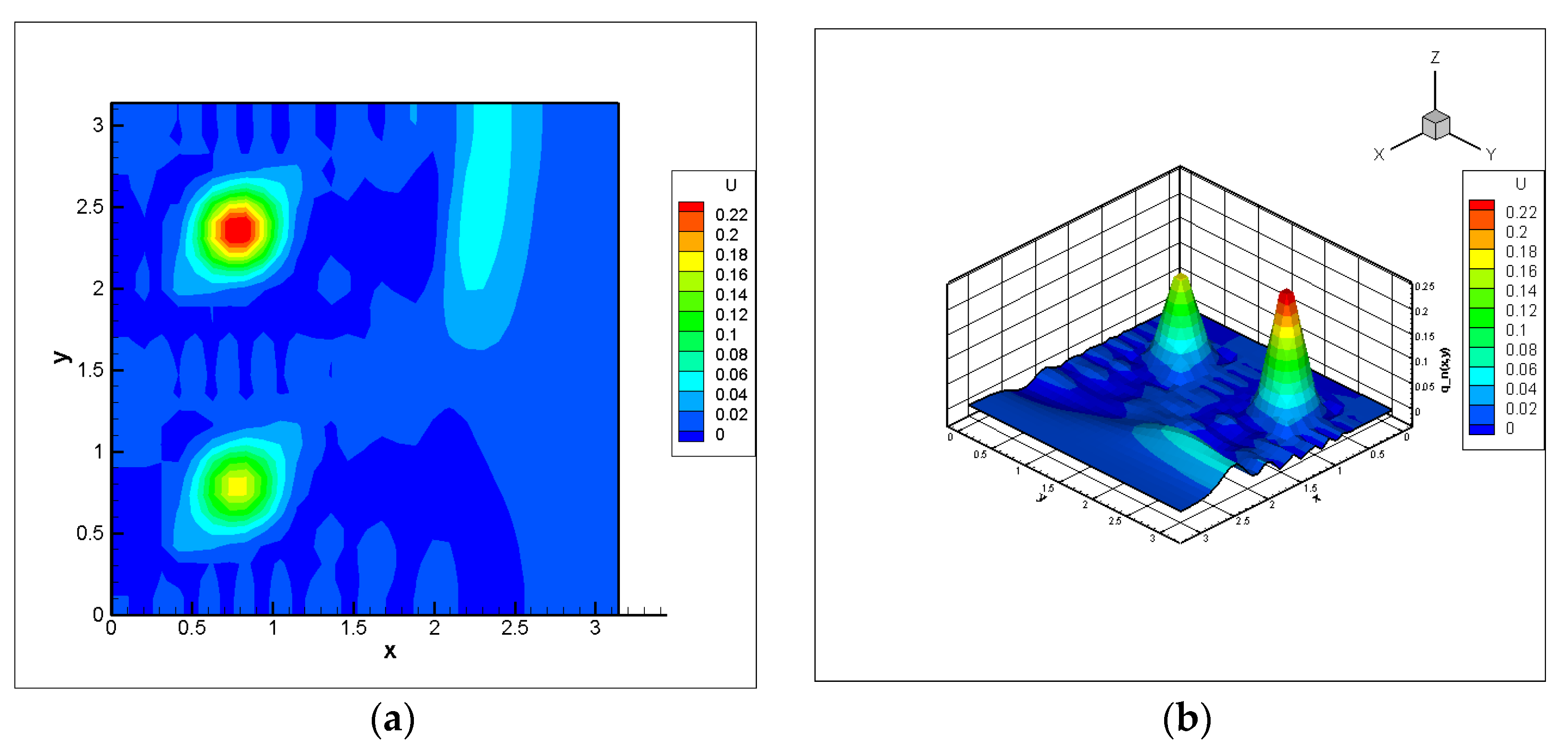
The results of the computational experiment are shown in Figure 1.

Figure 1a shows the function $q(x,y)$ as a two-dimensional heat map, which allows local changes in areas of high or low intensity to be clearly seen. This format is convenient for analyzing breakpoints, as well as for visual comparison with a known standard.

In Figure 1b, the same function is displayed in three dimensions, where the vertical axis reflects the amplitude $q(x,y)$. This allows one to visually assess the shape of the reconstructed surface and ensure that the spatial structure corresponds to the expected physical characteristics. A 3D visualization is particularly useful when interpreting wave processes in a multidimensional environment.

Thus, the use of both 2D and 3D graphs contributes to a more comprehensive assessment of the quality of the reconstructed function and highlights important aspects of the numerical method.

For the numerical solution of the direct problem, an explicit second-order precision time and space difference scheme is used. The explicit scheme is simple to implement and easily amenable to parallel processing, which makes it attractive for large-scale tasks. Similarly, as for the direct problem, it is possible to formulate the corresponding difference scheme and numerical solution algorithm for the conjugate problem. The construction technique remains the same: approximations of derivatives with respect to time and spatial variables are used, and boundary and initial conditions are also considered.

3.2. Quaternionic Fourier Transforms

Quaternionic Fourier transforms (QFT) are a powerful tool for analyzing and processing signals and images. Their use opens up new possibilities for working with three-dimensional and four-dimensional data, expanding our knowledge and methods in the field of digital signal and image processing. Since in the classical case, the Fourier transform decomposes a function into a sum of exponentials, the quaternionic Fourier transform allows you to take into account multidimensional dependencies using quaternionic exponentials.

Definition 2. 

Let $fϵL^1(R^2,H)$. The QFT transformation for $f$ is a function of ${\mathcal{F}}_q\left\{f\right\}:R^2\to H$, which is defined by the following formula:

$${\mathcal{F}}_q\left\{f\right\}\left(\omega \right)={\int }_{R^2}f\left(x\right)e^{-{\displaystyle \frac{i+j+k}{\sqrt{3}}}·\omega ·x}d{x}_{1}d{x}_2,$$

for $fϵL^2(R^2,H)$,${\mathcal{F}}_q\left\{f\right\}ϵL^1(R^2,H)$, the inverse QFT is defined as

$${\mathcal{F}}_q^{-1}\left[{\mathcal{F}}_q\left\{f\right\}\right]\left(x\right)={\displaystyle \frac{1}{{\left(2\pi \right)}^2}}{\int }_{R^2}{\mathcal{F}}_q\left\{f\right\}\left(\omega \right)e^{{\displaystyle \frac{i+j+k}{\sqrt{3}}}·\omega ·x}d{\omega }_{1}d{\omega }_2.$$

$\omega =\left({\omega }_1,{\omega }_2\right)$− frequencies in spatial variables$x=\left(x_1,x_2\right)$.

To solve this thermoacoustic problem related to the propagation of acoustic pressure and the calculation of the absorption coefficient of electromagnetic radiation, the QFT can be used. In thermoacoustic processes, the analysis of wave phenomena that occur during energy absorption and redistribution plays a key role. The use of QFT makes it possible to effectively study multidimensional wave equations by representing the dynamics of acoustic pressure in the frequency domain. This transformation takes into account not only the amplitude characteristics of the waves, but also their gradient and rotary structures, which is especially important when studying the propagation of acoustic waves in three-dimensional media with inhomogeneous parameters [17].

Consider the following problem in the domain $\mathrm{\Omega }=\left(0,\pi \right)\times \left(0,\pi \right)\times \left(0,T\right)$:

$$u_{tt}=u_{xx}+u_{yy}, \left(x,y,t\right)\in \mathrm{\Omega },$$

(29)

$$u\left(x,y,0\right)=q\left(x,y\right), { u}_t\left(x,y,0\right)=0, x\in \left[0,\pi \right],y\in \left[0,\pi \right].$$

(30)

Using the tabular formulas of the QFT of the Laplace operator and the multiplication rules, we obtain the following:

$$-{\mathcal{F}}_q\left\{{\displaystyle \frac{{\partial }^{2}u}{\partial t^2}}\right\}\left(\omega ,t\right)=-\left({\mathcal{F}}_q\left\{u\right\}\left(\omega ,t\right){\left({\displaystyle \frac{i+j+k}{\sqrt{3}}}{\omega }_1\right)}^2+{\mathcal{F}}_q\left\{u\right\}\left(\omega ,t\right){\left({\displaystyle \frac{i+j+k}{\sqrt{3}}}{\omega }_2\right)}^2\right),$$

$${\displaystyle \frac{d^2{\mathcal{F}}_q\left\{u\right\}\left(\omega ,t\right)}{d{t}^2}}=\left({\omega }_1^2+{\omega }_2^2\right){\mathcal{F}}_q\left\{u\right\}\left(\omega ,t\right),$$

$${\mathcal{F}}_q\left\{u\left(x,y,0\right)\right\}={\mathcal{F}}_q\left\{u\right\}\left(\omega ,0\right)={\mathcal{F}}_q\left\{q\right\}\left(\omega \right),$$

$${\mathcal{F}}_q\left\{{ u}_t\left(x,y,0\right)\right\}={\displaystyle \frac{d{\mathcal{F}}_q\left\{u\right\}}{dt}}\left(\omega ,0\right)=0.$$

By introducing the notation ${\mathcal{F}}_q\left\{u\right\}\left(\omega ,t\right)=y\left(t\right)$, we write the equation as follows:

$${\displaystyle \frac{d^{2}y}{d{t}^2}}-\left({\omega }_1^2+{\omega }_2^2\right)y=0,$$

$$y\left(0\right)={\mathcal{F}}_q\left\{q\right\}\left(\omega \right),{\displaystyle \frac{dy}{dt}}\left(0\right)=0.$$

An ordinary second-order differential equation with initial conditions, the solution of which has the form:

$${\mathcal{F}}_q\left\{u\right\}\left(\omega ,t\right)={\mathcal{F}}_q\left\{q\right\}\left(\omega \right)\cos \left(\sqrt{{\omega }_1^2+{\omega }_2^2}t\right).$$

To find a solution in physical space, we use the inverse QFT:

$$u\left(x,y,t\right)={\mathcal{F}}_q^{-1}\left[{\mathcal{F}}_q\left\{u\right\}\left(\omega ,t\right)\right]\left(x,y,t\right).$$

This section discusses an approach to solving a two-dimensional wave equation with initial conditions based on the application of QFT. The use of QFT made it possible to move from a differential equation in physical space to its algebraic representation in the frequency domain, which greatly simplified the analysis and led to the analytical expression of the solution in terms of cosine modes.

The proposed method has several advantages. Firstly, it allows us to naturally take into account the multidimensional structure of wave processes, which is especially important when analyzing complex media. Secondly, the representation of the solution in the frequency domain makes it possible to use spectral methods to further study the characteristics of the wave field, including dispersion properties and attenuation.

Thus, the quaternion Fourier transform is a powerful tool for solving problems related to wave propagation, especially in media with inhomogeneous parameters. This approach can be useful in various fields of science and technology, such as acoustics, electromagnetic waves, and quantum systems, where it is important to take into account the spatial and frequency dependences of wave processes.

3.3. Numerical Calculations Using the Quaternion Fourier Transform (QFT) Method

The quaternion Fourier transform (QFT) is a generalization of the classical Fourier transform that allows you to work with multidimensional and vector data. Unlike the standard method used to solve scalar wave equations, QFT takes into account the general structures of wave processes, which makes it particularly useful in analyzing complex wave phenomena, including thermoacoustics and electromagnetic wave propagation.

Various methods can be used to solve this problem numerically, including finite difference schemes, spectral methods, and Fourier transforms. The QFT has an advantage in representing multidimensional data since it naturally takes into account spatial dependencies and allows efficient analysis of vector fields. This makes it particularly useful in applications involving acoustic and electromagnetic waves.

Figure 2 shows a graph of the quaternion Fourier transform of the function $q\left(x,y\right)$, decomposed into four components:

$${\mathcal{F}}_q\left\{q\right\}\left({\omega }_x,{\omega }_y\right)=Q_0\left({\omega }_x,{\omega }_y\right)+i{Q}_1\left({\omega }_x,{\omega }_y\right)+j{Q}_2\left({\omega }_x,{\omega }_y\right)+k{Q}_3\left({\omega }_x,{\omega }_y\right).$$

The analysis has shown that the quaternion Fourier transform is a powerful tool for the numerical solution of multidimensional wave problems. Unlike the classical Fourier series expansion, QFT allows you to work naturally with vector fields and take into account spatial dependencies. At the same time, the method remains stable and accurate when analyzing complex environments. Therefore, this tool was used in the numerical solution of the direct problem in order to fully take into account all the characteristics of the wave process.

4. Discussion

4.1. Numerical Solution of the Inverse Problem

When numerically modeling inverse problems, it is a common mistake to use the same numerical scheme and discretization both to solve the direct problem and to reconstruct the initial data. This practice leads to an overestimation of the accuracy of the method, since it does not reflect the actual measurement conditions and possible errors [18,19]. To avoid this error, various numerical approaches should be used to generate and interpret data, as well as to investigate the stability of the method used.

In this paper, we conduct a numerical experiment for a model problem. At the first stage, a direct problem is solved with a known function $q_T\left(x,y\right)$, as a result of which the value of the solution on the boundary is determined: $u\left(0,y,t\right)=f\left(y,t\right)$. For this, the QFT method is used, which provides a spectral representation of the solution. At the next stage, to restore the original function using additional information $f\left(y,t\right)$, the inverse problem is solved using the accelerated Nesterov method (

Table 1. The evolution of the value of the functional $J\left(q_n\right)$ and standard errors $‖q_T-q_n‖,‖u_T-u_n‖$ on different iterations of the Nesterov method.

Iteration	$$\mathit{J}\left({\mathit{q}}_{\mathit{n}}\right)$$	$$‖{\mathit{q}}_{\mathit{T}}-{\mathit{q}}_{\mathit{n}}‖$$	$$‖{\mathit{u}}_{\mathit{T}}-{\mathit{u}}_{\mathit{n}}‖$$
0	0.0122086966	0.0091833454	0.0022304495
1	0.0066524126	0.00790955167	0.0018279980
10	7.9931729747 × 10−5	0.00539634584	0.0010478261
50	9.0956035731 × 10−6	0.00498284483	0.0009636881
100	3.8247066028 × 10−6	0.00492036141	0.0009497397
500	7.9913306446 × 10−7	0.00483146561	0.0009317223

). This method is used in combination with an explicit second-order precision difference scheme for the numerical solution of direct and conjugate problems.

Numerical results show that the solution of the inverse problem has not been fully recovered (Figure 3). This indicates that the available additional information is insufficient to unambiguously determine the source data. In this regard, as an additional condition, another function is introduced on the boundary in the form $u\left(\pi ,y,t\right)=f_2\left(y,t\right)$, which makes it possible to increase the stability and completeness of the recovery.

Due to the need to improve the quality of recovery, we will consider the modified objective functionality.

$$J\left(q_n\right)=\underset{0}{\overset{T}{\int }}\underset{0}{\overset{\pi }{\int }}{\left(u\left(0,y,t;q_n\right)-f_1\left(y,t\right)\right)}^{2}dydt+\underset{0}{\overset{T}{\int }}\underset{0}{\overset{\pi }{\int }}{\left(u\left(\pi ,y,t;q_n\right)-f_2\left(y,t\right)\right)}^{2}dydt$$

(31)

Accordingly, the formulation of the associated problem changes, taking into account the new conditions.

$${\psi }_{tt}={\psi }_{xx}+{\psi }_{yy},$$

(32)

$$\psi \left(x,y,T\right)=0, {\psi }_t\left(x,y,T\right)=0,$$

(33)

$${\psi }_x\left(0,y,t\right)=2\left(u\left(0,y,t\right)-f_1\right), {\psi }_x\left(\pi ,y,t\right)=-2\left(u\left(\pi ,y,t\right)-f_2\right),$$

(34)

$${\psi }_y\left(x,0,t\right)={\psi }_y\left(x,\pi ,t\right)=0.$$

(35)

To numerically solve the updated problem, an additional computational experiment is conducted using the accelerated Nesterov algorithm (

Table 2. The evolution of the value of the functional $J\left(q_n\right)$ and standard errors $‖q_T-q_n‖,‖u_T-u_n‖$ on different iterations of the method Nesterov with $f_2\left(y,t\right)$.

Iteration	$$\mathit{J}\left({\mathit{q}}_{\mathit{n}}\right)$$	$$‖{\mathit{q}}_{\mathit{T}}-{\mathit{q}}_{\mathit{n}}‖$$	$$‖{\mathit{u}}_{\mathit{T}}-{\mathit{u}}_{\mathit{n}}‖$$
0	0.0184060952	0.0109895446	0.0022304495
1	0.0178195672	0.0108379340	0.0021989219
100	0.0002271009	0.0026551399	0.0005048771
500	9.1380318027 × 10−6	0.0012533504	0.0002370370
1000	1.8142271044 × 10−6	0.0009725205	0.0001806675
1500	8.8569469994 × 10−7	0.0008676791	0.0001593380

).

The numerical experiment shows that adding an additional condition on the boundary significantly increases the accuracy of restoring the original function $q(x,y)$ in the inverse problem. In particular, when using only one boundary condition, the reconstruction turns out to be incomplete and sensitive to numerical errors. However, the introduction of additional information in the form of a second boundary condition, for example $u\left(\pi ,y,t\right)=f_2\left(y,t\right)$, significantly improves the quality of reconstruction (Figure 4).

Thus, it can be reasonably concluded that the availability of more complete and diverse additional information contributes to improving the stability and accuracy of the numerical solution of the inverse problem. This confirms the following general theoretical pattern: the more information is available when solving an ill-posed problem, the more reliable and stable the reconstructed solution will be.

4.2. Comparative Analysis with Existing Methods

Solving inverse problems for the wave equation is traditionally associated with the use of various regularization methods. The most widely used is Tikhonov regularization, which ensures the stability of the solution in the presence of noise. Comparative analysis shows that methods based on Tikhonov regularization and Carleman estimates have their advantages, but also have certain limitations compared to the approach we proposed. The article [20] proposes a Bayesian interpretation of Tikhonov distributed regularization, which allows formalizing a priori information and improving the stability of the solution. However, this approach requires an accurate a priori statistical model and can be sensitive to the choice of regularization parameters, especially for high-dimensional problems. At the same time, the method in the article [21] uses Carleman estimates to prove the stability of source reconstruction in the wave equation, which provides strict theoretical guarantees. However, the practical implementation of the method requires high requirements for numerical approximation and the construction of weight functions.

Back projection methods [22], often used in computer tomography and acoustics, assume the presence of an analytical or approximate form of the inverse operator. Although these methods are easy to implement and work well with complete information, they are sensitive to missing data and noise. The proposed method does not require explicit inversion, but is based on solving the adjoint problem with subsequent calculation of the functional gradient, which makes it more flexible with partial and imprecise data.

A special feature of this work is the use of the quaternion Fourier transform (QFT) [11], which allows taking into account the vector structure of the field and effectively analyzing the spectral characteristics of multicomponent signals. This is particularly relevant in problems related to fractal geometry or anomalous diffusion, where classical transformations are not expressive enough [23].

In the work of Kabanikhin et al. (2013) [7], an inverse thermoacoustic problem is considered, where the method of simple iteration with the classical formulation of the initial-boundary value problem is used. The algorithm takes into account three variants of additional data: (1) one boundary condition, (2) two boundary conditions, and (3) three boundary conditions. It is shown that an increase in the number of measurements significantly improves the accuracy of the absorption coefficient reconstruction. For each variant, a numerical experiment is carried out, in which the results of the source function reconstruction at different iterations are compared from 307 to 500 steps, which serves as a kind of regularization. In contrast, this work employs a gradient method of functional minimization using the accelerated Nesterov algorithm, as well as the quaternion Fourier transform, which allows for the efficient processing of multidimensional signals. In addition, in the author’s numerical experiments, the additional condition is introduced gradually, and it is shown that adding a second boundary condition leads to a sharp improvement in recovery. Thus, the method proposed in this study offers greater flexibility and spectral expressiveness, while Kabakikhin’s approach demonstrates the classical stability and clarity of the iterative process under the various levels of a priori information.

Unlike other approaches, our work combines the numerical efficiency of gradient methods (including the accelerated Nesterov algorithm) with the high accuracy of spectral analysis provided by the quaternion Fourier transform (QFT). This allows us to effectively reconstruct multidimensional wave fields and take into account complex spatial dependencies, which is particularly important while working with inhomogeneous media. In addition, our work proves the existence of the Frechet derivative for the functional, which increases the rigor of the used numerical method. Thus, the proposed method demonstrates both theoretical validity and high computational efficiency in solving the inverse problem of thermoacoustics.

5. Conclusions

In this paper, we consider the initial boundary value problem for the wave equation in the absence of one of the initial conditions, which leads to the formulation of the inverse problem. A generalized solution to the direct problem was formulated, its correctness was proved, and an a priori estimate of the solution was obtained. The inverse problem was reduced to an optimization problem, where gradient descent methods were used to minimize the functional. In this regard, the formulation of the conjugate problem was obtained, and the gradient of the target functional was computed. In addition, it was shown that the functional has a Frechet derivative.

The accelerated Nesterov algorithm was used for the effective implementation of the numerical method. A special feature of this work was the application of the QFT in the numerical solution of a direct problem, which allowed us to obtain a deeper spectral representation of the solution.

A computational experiment was conducted for the inverse problem. The results showed that in the presence of a single additional condition, the restoration of function remains incomplete. This highlights the importance of the quantity and quality of additional information. To increase the stability of the recovery, it was proposed to introduce another boundary condition in the form $u\left(\pi ,y,t\right)=f_2\left(y,t\right)$, which significantly improved the result. The findings confirm that the more reliable information is used to solve the inverse problem, the higher the accuracy and stability of the reconstructed solution.

In this study, we consider the problem of numerical reconstruction of the initial condition for the wave equation using the gradient method and the quaternion Fourier transform (QFT). Despite the successful implementation of the proposed approach, it has a number of limitations. The method has shown high sensitivity to the amount of available additional information. The numerical experiment demonstrated that, with only one boundary condition available, the reconstruction of the original function remains incomplete, which indicates the need to expand the information at the boundary of the domain.

In addition, the method’s efficiency depends significantly on the properties of the function being restored. The most reliable results are obtained when the method is applied to smooth and regular functions. In cases where the data contains noise or has discontinuities, additional adaptation of the method is required, for example, by using filtering or special regularizers. It is also worth noting that the implementation of the quaternion Fourier transform in multidimensional problems is characterized by high computational complexity, which requires the use of accelerated algorithms and efficient computational schemes.

Further research directions may be related to the expansion of the proposed approach to more complex classes of problems, including models with a fractal structure and fractional calculus, which is particularly relevant when modeling processes in heterogeneous and memory-effect media. Also promising is the development of robust hybrid methods combining the quaternion approach with Tikhonov regularization or Bayesian techniques, which will improve the stability and accuracy of restoration in conditions of limited and noisy data.

References

1. Pikalov, V.V.; Preobrazhensky, N.G. Computational tomography and physical experiment. Successes Phys. Sci. 1983, 141, 469–498. [Google Scholar]
2. Pikalov, V.V.; Preobrazhensky, N.G. Reconstructive Tomography in Gas Dynamics and Plasma Physics; Nauka Publ.: Novosibirsk, Russia, 1987. [Google Scholar]
3. Pikalov, V.V.; Melnikova, T.S. Low-Temperature Plasma; Plasma tomography; Nauka Publ. Siberian Publishing Company of the Russian Academy of Sciences: Novosibirsk, Russia, 1995; Volume 13. [Google Scholar]
4. Romanov, V.G. Inverse Problems of Mathematical Physics; Nauka Publ.: Novosibirsk, Russia, 1984. [Google Scholar]
5. Romanov, V.G. Integral geometry on geodesics of an ichotropic Riemannian metric. In Doklady Akademii Nauk; Russian Academy of Sciences: Novosibirsk, Russia, 1978; Volume 241, pp. 290–293. [Google Scholar]
6. Sharafutdinov, V.A. Integral Geometry of Tensor Fields; Walter de Gruyter: Berlin, Germany, 2012; Volume 1. [Google Scholar]
7. Kabanikhin, S.I.; Krivorot’ko, O.I.; Shishlenin, M.A. A numerical method for solving an inverse thermoacoustic problem. Numer. Anal. Appl. 2013, 6, 34–39. [Google Scholar] [CrossRef]
8. Nurseitov, D.B.; Kassenov, S.E. Numerical solution of initial-boundary problem for the Helmholtz equation on “discretization-optimization”. Bull. Karaganda Univ.-Math. 2014, 75, 114–120. [Google Scholar]
9. Bektemesov, M.A.; Kabanikhin, S.I.; Nurseitov, D.B.; Kasenov, S.Y. Numerical solution of the initial-boundary value problem for the Helmholtz equation. Sib. Elektron. Mat. Izvestia Sib. Electronic Math. Rep. 2014, 11, 4–21. [Google Scholar]
10. Kasenov, S.E.; Tleulesova, A.M.; Sarsenbayeva, A.E.; Temirbekov, A.N. Numerical Solution of the Cauchy Problem for the Helmholtz Equation Using Nesterov’s Accelerated Method. Mathematics 2024, 12, 2618. [Google Scholar] [CrossRef]
11. Sangwine, S.J.; Ell, T.A. Hypercomplex Fourier transforms of color images. In Proceedings of the 2001 International Conference on Image Processing (Cat. No. 01CH37205), Thessaloniki, Greece, 7–10 October 2001; Volume 1, pp. 137–140. [Google Scholar]
12. Hitzer, E.M.S. Quaternion fourier transform on quaternion fields and generalizations. Adv. Appl. Clifford Algebras 2007, 17, 497–517. [Google Scholar] [CrossRef]
13. Ell, T.A.; Le Bihan, N.; Sangwine, S.J. Quaternion Fourier Transforms for Signal and Image Processing; John Wiley & Sons: Hoboken, NJ, USA, 2014. [Google Scholar]
14. Kabanikhin, S.I. Inverse and Ill-Posed Problems: Theory and Applications; de Gruyter: Berlin, Germany, 2011. [Google Scholar]
15. Kasenov, S.; Nurseitova, A.; Nurseitov, D. A conditional stability estimate of continuation problem for the Helmholtz equation. In AIP Conference Proceedings; AIP Publishing: Melville, NY, USA, 2016; Volume 1759. [Google Scholar]
16. Samarsky, A.A.; Gulin, A.V. Numerical Methods; Nauka: Moscow, Russia, 1989; 432p. (In Russian) [Google Scholar]
17. Kasenov, S.E.; Demeubayeva, Z.E.; Temirbekov, N.M.; Temirbekova, L.N. Solution of the Optimization Problem of Magnetotelluric Sounding in Quaternions by the Differential Evolution Method. Computation 2024, 12, 127. [Google Scholar] [CrossRef]
18. Hansen, P.C. Discrete Inverse Problems: Insight and Algorithms; Society for Industrial and Applied Mathematics: Philadelphia, PA, USA, 2010. [Google Scholar]
19. Hamarik, U.; Palm, R. Comparison of stopping rules in conjugate gradient type methods for solving ill-posed problems. In Proceedings of the MMA2005 Proceedings: 10th International Conference Mathematical Modelling and Analysis, 2nd International Conference Computational Methods in Applied Mathematics, Trakai, Lithuania, 1–5 June 2005; pp. 285–291. [Google Scholar]
20. Calvetti, D.; Somersalo, E. Distributed Tikhonov regularization for ill-posed inverse problems from a Bayesian perspective. Comput. Optim. Appl. 2025, 91, 541–572. [Google Scholar] [CrossRef]
21. Boulakia, M.; de Buhan, M.; Delaunay, T.; Imperiale, S.; Moireau, P. Solving inverse source wave problemfrom Carleman estimates to observer design. In Mathematical Control and Related Fields; American Institute of Mathematical Sciences (AIMS): Springfield, MO, USA, 2024. [Google Scholar]
22. Natterer, F. The Mathematics of Computerized Tomography; SIAM: Philadelphia, PA, USA, 2001. [Google Scholar]
23. Tarasov, V.E. Fractional Dynamics: Applications of Fractional Calculus to Dynamics of Particles, Fields and Media; Springer: New York, NY, USA, 2011. [Google Scholar]
Figure 1. Results of numerical simulation of the direct problem. (a) The function q ( x , y ) in a two-dimensional representation. (b) The function q ( x , y ) in a three-dimensional representation. (c) The function u x , y , T in a two-dimensional representation. (d) The function u x , y , T in three-dimensional representation. (e) The function u 0 , y , t in a two-dimensional representation. (f) The function u 0 , y , t in three-dimensional representation.
Fractalfract 09 00370 g001
Figure 2. Graph of the function F q q ω x , ω y . (a) Q 0 ω x , ω y . (b) Q 1 ω x , ω y . (c) Q 2 ω x , ω y . (d) Q 3 ω x , ω y .
Fractalfract 09 00370 g002
Figure 3. The reconstructed function q n x , y of the Nesterov method. (a) The reconstructed function q n in a two-dimensional representation. (b) The reconstructed function q n in the three-dimensional representation.
Fractalfract 09 00370 g003
Figure 4. The reconstructed function q n x , y of the method of Nesterov with f 2 y , t . (a) The reconstructed function q n in a two-dimensional representation. (b) The reconstructed function q n in the three-dimensional representation.
Fractalfract 09 00370 g004