Advanced Stability Analysis for Fractional-Order Chaotic DC Motors Subject to Saturation and Rate Limitations

Abstract

Chaotic behavior and memory-dependent dynamics in fractional-order brushless DC motors (FOBLDCMs) pose significant challenges for robust and stable control design, particularly when physical constraints such as actuator saturation and rate limitations are present. Existing control frameworks often neglect these nonlinear limitations, resulting in performance degradation and potential instability in practical applications. Motivated by these challenges, this paper presents a comprehensive Lyapunov-based stability and control synthesis framework for FOBLDCMs within the fractional-order (FO) range $0<v<1$. The proposed methodology employs indirect, direct, and composite Lyapunov functions to derive sufficient stability conditions under four scenarios: unconstrained input, saturation-only, rate-limited-only, and combined constraints. For each case, a family of stabilizing controllers is designed to explicitly handle the respective limitations. To the best of our knowledge, this is the first study to rigorously address both saturation and rate limitations in the control design of FO chaotic systems. Numerical simulations confirm that the proposed controllers significantly improve performance over existing methods. Specifically, the unconstrained controller achieves a notable reduction in control energy (from $2.72\times {10}^5$ to $1.83\times {10}^5$), a 26.3% decrease in maximum control effort, and enhanced or comparable tracking accuracy, as indicated by lower ISE and RMSE values. These results highlight the robustness and practical applicability of the proposed control framework for real-world FO electromechanical systems.

1. Introduction

Fractional calculus (FC), an extension of classical integer-order calculus, offers a powerful framework for capturing memory and hereditary properties in complex dynamical systems. By introducing non-local operators, FC enables more accurate descriptions of processes where current states depend not only on present conditions but also on historical trajectories. This capability makes it highly relevant for modeling and analysis in control engineering, signal processing, viscoelasticity, and beyond. Recent works have increasingly leveraged FC to study physical and engineering systems where conventional integer-order models fall short [1,2,3,4]. Particularly, the mathematical richness of fractional-order (FO) derivatives has facilitated nuanced modeling of nonlinear, chaotic, and high-dimensional systems.

1.1. Motivation and Background

FO modeling techniques have gained substantial attention across various engineering disciplines due to their superior ability to capture complex dynamics with fewer parameters and enhanced accuracy compared to their classical integer-order counterparts [5,6,7]. These methods have proven particularly useful in analyzing chaotic systems, where nonlinearities and sensitivity to initial conditions demand more refined modeling tools. Prominent examples include the FO Lorenz, Chen, and Lü systems, as well as FO models of brushless DC motors (BLDCMs) [8,9,10,11]. The pioneering work by Hemati [12] introduced chaotic dynamics in BLDCMs, while subsequent studies such as [13] utilized both analytical and computational tools to characterize chaotic regimes and design stabilizing strategies. Researchers in [11] further extended the analysis by deriving bifurcation properties of FO BLDCMs (FOBLDCMs), and detailed investigations in [14,15,16] explored their bifurcation structures and qualitative behaviors. These studies confirmed that while chaos poses risks to the performance and reliability of actuators, it can be rigorously studied and mitigated through advanced modeling approaches.

In terms of control strategies for FO chaotic systems, numerous methods have been proposed within the FO domain ($0<v<1$). For instance, Ref. [17] proposed a Lyapunov-based stabilization approach leveraging a single state variable. In a related work, the authors of [18] analyzed the stabilization of a nonlinear FOBLDCM using Caputo derivatives, supported by mathematical tools such as the Laplace transform, the Mittag–Leffler function, Jordan decomposition, and Grönwall’s inequality. Moreover, Ref. [19] introduced a novel adaptive control strategy based on the Immersion and Invariance (I&I) theorem and fuzzy systems to synchronize chaotic BLDCM dynamics with desired trajectories, especially for electric vehicle applications. Alternative formulations such as FO operators—including the Caputo, Caputo–Fabrizio, and Atangana–Baleanu definitions—have also been employed in modeling and control, as seen in [20]. Sensorless control approaches have also been developed for high-speed BLDCMs, using digital signal processors (DSPs) to enhance commutation accuracy, as discussed in [21]. Bifurcation-based anti-control techniques were proposed in [22], where various external periodic and constant signals were shown to influence complex bifurcation structures, including Hopf, Bogdanov–Takens, and period-doubling types. Additionally, works such as [23] explored single-input stabilization, [24] analyzed quasi-Mittag–Leffler stability for distributed-order systems, and the authors’ contributions in [25] addressed delay-induced instability in FO power systems using Lyapunov functionals. However, many of these studies still assume idealized conditions and often neglect key practical constraints such as actuator saturation and input rate limitations—challenges that are critical in real-world applications.

1.2. Modeling with Input Constraints

The integration of actuator saturation into FO system modeling yields a block-oriented structure, notably resembling Hammerstein models, where a static nonlinearity (saturation) precedes a linear or nonlinear FO dynamic system. This opens a promising avenue for system identification and control. Recent contributions in FO Hammerstein modeling include the development of smoothed functional algorithms with norm-limited update vectors for the identification of continuous-time FO Hammerstein systems [26]. Similarly, iterative parameter estimation methods were applied in [27] to FO Hammerstein systems under colored noise. However, these approaches primarily focus on identification, not stabilization or constrained control design. The current work seeks to bridge this gap by formulating a control-oriented FO Hammerstein framework for systems with both amplitude and rate limitations, a direction previously unexplored.

Furthermore, in recent years, significant advancements have been made in the control of BLDCMs, particularly through the application of FO control theory. Classical control strategies have been extended with robust, adaptive, and intelligent features to handle system nonlinearities, parameter uncertainties, and external disturbances more effectively. For instance, the authors of [28] proposed a finite-time super-twisting algorithm based on recurrent neural networks for FO systems, demonstrating improved transient and steady-state performance. In another direction, Ref. [29] tackled the challenges of rate-limited control in FO systems by introducing flat phase constraints derived from Bode integrals. Furthermore, Ref. [30] presented a novel integration of active disturbance rejection control (ADRC) with compensation for actuator rate limitations, validating its effectiveness through experimental results on benchmark systems. Despite these promising developments, most control approaches for FO chaotic systems—including BLDCMs—do not simultaneously consider both actuator saturation and rate limitations, which are frequently encountered in practice. Instead, these limitations are typically addressed separately, with many designs assuming ideal actuator behavior.

A contribution addressing input constraints can be found in the work of Alavian Shahri et al. [31,32,33,34,35], who analyzed saturation effects on control inputs in both linear and nonlinear systems, including cases with and without time delays. These studies offered valuable insights into the impact of input bounds in FO systems. However, they primarily focused on saturation constraints, leaving rate limitations either unaddressed or only marginally considered. Moreover, their scope did not encompass chaotic dynamics or FOBLDCMs specifically, where the interaction of saturation and rate constraints plays a critical role in achieving safe and stable operation.

Beyond constraint handling, another common limitation in current control designs lies in the underlying assumptions regarding system observability and feedback availability. Many approaches rely heavily on direct Lyapunov methods and presume access to full state measurements or multiple sensors—conditions often impractical in embedded or resource-limited systems. Additionally, few controllers incorporate physical actuator characteristics such as limited bandwidth or maximum permissible control effort during the synthesis process. Neglecting these constraints can result in suboptimal tracking performance, delayed response, or even destabilization of the closed-loop system under real-world operating conditions.

1.3. Gap and Contribution Overview

To the best of our knowledge, no prior work has systematically addressed the stabilization of FO chaotic BLDCMs under both amplitude saturation and rate-limited control inputs. Motivated by this practical need, this paper proposes a unified framework for stability analysis and controller synthesis using novel Lyapunov candidates for various constrained scenarios. The proposed approach accommodates single, dual, and triple input cases, reducing sensor dependency while ensuring robust performance under physical limitations. By extending FO system modeling to include block-oriented nonlinearities, this research also lays a theoretical foundation for FO Hammerstein-type control architectures.

1.4. Main Contributions

The primary contributions of this work are summarized as follows:

• Unified stability framework: A comprehensive Lyapunov-based stability framework is developed for FO chaotic BLDCMs under input constraints including saturation, rate limits, and their combination. To our knowledge, this is the first study that considers both rate and amplitude limitations simultaneously in FO chaotic control design.
• Novel Lyapunov candidates: Tailored Lyapunov functions are constructed for each control scenario—unconstrained, saturated, rate-limited, and jointly constrained—based on a combination of direct and indirect Lyapunov methods.
• Input-constrained controller design: Multiple controller configurations are derived from stability conditions, enabling implementations with reduced sensor requirements (single-, double-, and triple-input variants).
• Benchmark validation: The effectiveness of the proposed framework is demonstrated through extensive simulations on FOBLDCMs with varying degrees of input constraints and nonlinear behavior.

1.5. Organization

The organization of this paper is as follows: Section 2 delineates the requisite definitions and preliminaries imperative for comprehending the concepts and methods employed in subsequent sections. Section 3 details the stability analysis and controller design methodologies, underscoring the introduced indirect Lyapunov method without and with limitations. Section 4 presents comprehensive simulation results, corroborating the efficacy of the proposed methods in stabilizing FOBLDCMs. Finally, Section 5 encapsulates the study, summarizing salient findings and suggesting potential trajectories for future exploration.

2. Preliminaries

In this section, the preliminary mathematical concepts are presented.

Definition 1 

([2]). The Caputo derivative of a smooth function, denoted by $g\left(t\right):{\mathbb{R}}^{+}⟶\mathbb{R}$, with an FO v, can be expressed as follows:

$${}_{t_0}{}^{C}D_t^{v}g\left(t\right)={\displaystyle \frac{1}{\Gamma \left(n-v\right)}}\underset{t_0}{\overset{t}{\int }}{\displaystyle \frac{g^{\left(n\right)}\left(\tau \right)}{{\left(t-\tau \right)}^{v-n+1}}}d\tau ,$$

(1)

where $n\in \mathbb{N}$, $n-1<v<n$, is the $n^{th}$ derivative of the function $g\left(t\right)$.

The Laplace transform of $g\left(t\right)$ can be expressed as follows:

$$\ell \left\{{}_{t_0}{}^{C}D_t^{v}g\left(t\right)\right\}=s^{v}G\left(s\right)-\sum _{k=0}^{n-1}{s}^{v-k-1}{g}^{\left(k\right)}\left(0\right).$$

(2)

Theorem 1 

([36,37]). The following equation satisfies the condition for any $s\in \mathbb{C}$ and $0<v<1$:

$$\underset{0}{\overset{\infty }{\int }}{\displaystyle \frac{{\mu }_v\left(\omega \right)}{s+\omega }}d\omega ={\displaystyle \frac{1}{s^v}},$$

(3)

where ${\mu }_v\left(\omega \right)={\displaystyle \frac{sin\left(v\pi \right)}{\pi {\omega }^v}}$.

By applying the Laplace transform to Equation (3), we obtain

$$\underset{0}{\overset{\infty }{\int }}{\mu }_v\left(\omega \right)e^{-\omega t}d\omega ={\displaystyle \frac{t^{v-1}}{\Gamma \left(v\right)}}.$$

(4)

Theorem 2 

([37]). The FO nonlinear differential equation ${}_{t_0}{}^{C}D_t^{v}y\left(t\right)=g\left(t\right)$ can be interpreted using the continuous-frequency-distributed model of the fractional integrator as follows:

$${\displaystyle \frac{\partial z\left(\omega ,t\right)}{\partial t}}=-\omega z\left(\omega ,t\right)+g\left(t\right),$$

(5)

In this context, the variable $z(\omega ,t)\in \mathbb{R}$ represents the frequency-distributed state, and the output $y\left(t\right)$ corresponds to the weighted integral of $z(\omega ,t)$.

$$y\left(t\right)=\underset{0}{\overset{\infty }{\int }}{\mu }_v\left(\omega \right)z\left(\omega ,t\right)d\omega ,$$

(6)

with $y\left(t\right)=0$ and $0<v<1$.

Lemma 1 

([38]). For any real matrices M and N of appropriate dimensions, the following inequality is satisfied for any scalar k:

$$MN+M^T{N}^T<kM{M}^T+k^{-1}N{N}^T$$

(7)

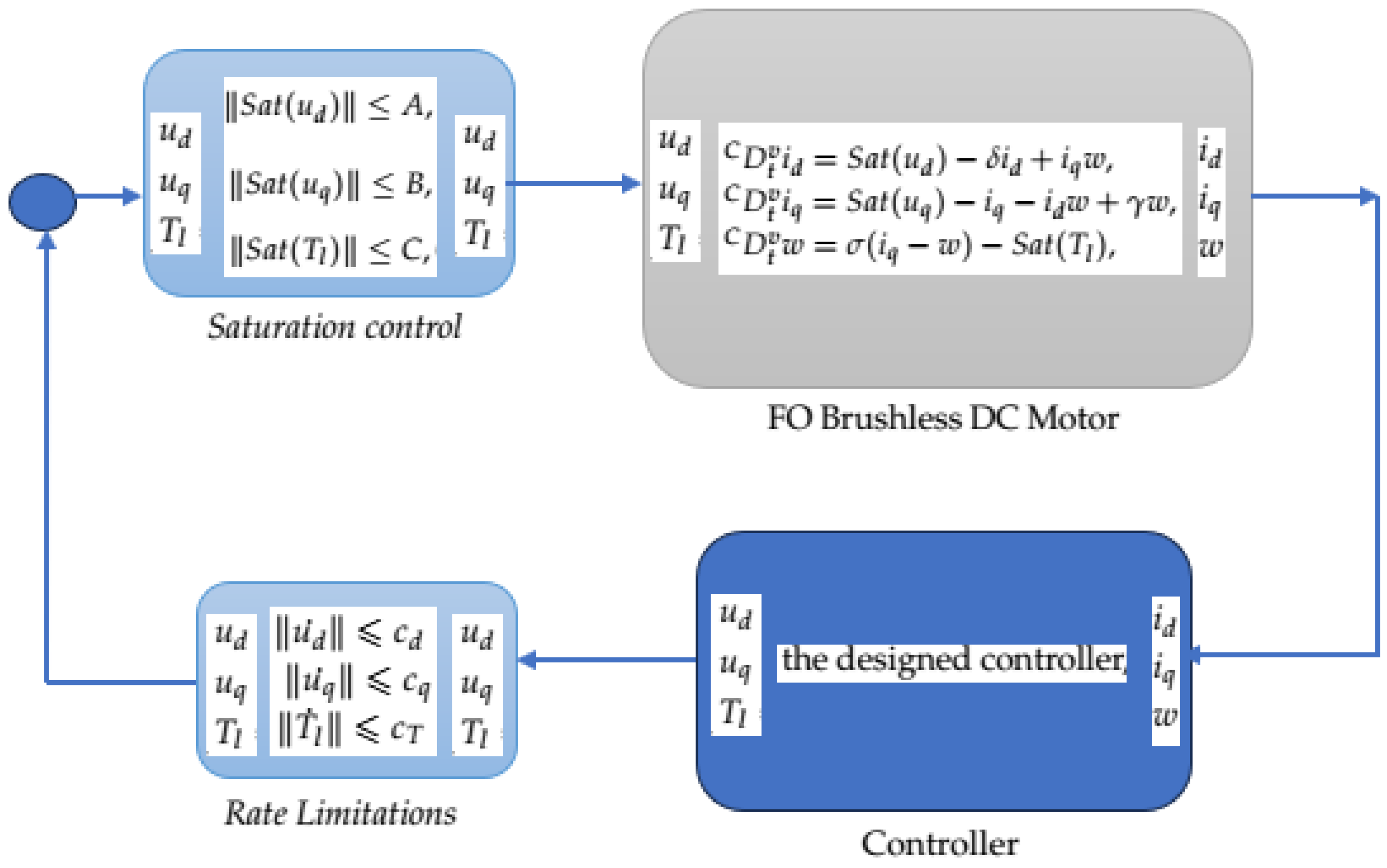
3. Main Results

Consider the FO brushless DC motor (FOBLDCM) described by the following equation [39]:

$$\left\{\begin{array}{c}{}^{C}D_t^v{i}_d=Sat\left(u_d\right)-\delta i_d+i_{q}w,\parallel \dot{u_d}\parallel ⩽c_d\hfill \\ {}^{C}D_t^v{i}_q=Sat\left(u_q\right)-i_q-i_{d}w+\gamma w,\parallel \dot{u_q}\parallel ⩽c_q\hfill \\ {}^{C}D_t^{v}w=\sigma (i_q-w)-Sat\left(T_l\right),\parallel \dot{T_l}\parallel ⩽c_T\hfill \end{array}\right.,0<v<1$$

(8)

where w, $i_q$, and $i_d$ represent the angular speed, quadrature-axis current, and direct-axis current of the motor, respectively. The system also includes positive parameters $\delta$, $\gamma$, and $\sigma$, which determine the specific dynamical behavior of the motor. Additionally, the controls $u_d$, $u_q$, and T play a role in governing the system dynamics. Furthermore, $c_d,c_q$, and $c_T$ are positive numbers that show rate limitation in specific inputs. Figure 1 shows the control system block diagram of the FOBLDCM. The function $Sat(·)$ represents the saturation function, defined as $Sat\left(r\right)=sign\left(r\right)Min(r,$ a), that has the saturation level a. This function is shown in Figure 2.

As a first step, we have to make some assumptions about the control input, as follows:

$$\parallel Sat\left(u_d\right)\parallel \le A,A\in R^{+}$$

(9)

$$\parallel Sat\left(u_q\right)\parallel \le B,B\in R^{+}$$

(10)

$$\parallel Sat\left(T_l\right)\parallel \le C,C\in R^{+}$$

(11)

The open-loop behavior of the FOBLDCM is illustrated in Figure 3 and Figure 4 for different values of the fractional derivative. Specifically, when $\sigma =4$, $\gamma =55$, and $\delta =0.875$, and with initial condition ${\left[\begin{array}{ccc}10& 3& -12\end{array}\right]}^T$, the system exhibits aperiodic, sudden, random, or morbid oscillations, indicating chaotic behavior. These chaotic oscillations can have detrimental effects on system stability. Therefore, it is of utmost importance to address the challenges posed by the chaotic FOBLDCM and develop effective control methods to stabilize the system.

3.1. No Limitation Control

We consider the present analysis step by step. In the first step, study Equation (8) without any limitation, as described by the following equation [39]:

$$\left\{\begin{array}{c}{}^{C}D_t^v{i}_d=u_d-\delta i_d+i_{q}w\hfill \\ {}^{C}D_t^v{i}_q=u_q-i_q-i_{d}w+\gamma w\hfill \\ {}^{C}D_t^{v}w=\sigma (i_q-w)-T_l\hfill \end{array}\right., 0<v<1$$

(12)

Theorem 3. 

The system described in Equation (12) can achieve global stability at the equilibrium point by implementing the following controller:

$$i_d{u}_d+i_q{u}_q+(\sigma +\gamma )w{i}_q-w{T}_l\le 0.$$

(13)

where $u_d$, $u_q$, and $T_l$ are the control inputs. By substituting this controller into Equation (12) and satisfying the inequality constraint given by Equation (13), then the closed loop system is asymptotically stable.

Note 1. 

Theorem 3 is satisfied with the necessary condition that none of the eigenstates, $i_d$ or $i_q$ or w, are included in the denominator of the designed controller.

Proof. 

Based on Theorem 2, we can alternatively express the system described by Equation (12) as

$$\left\{\begin{array}{c}{\displaystyle \frac{\partial z_1\left(\omega ,t\right)}{\partial t}}=-\omega z_1(\omega ,t)+u_d-\delta i_d+i_{q}w\hfill \\ i_d=\underset{0}{\overset{\infty }{\int }}{\mu }_v\left(\omega \right)z_1(\omega ,t)d\omega ,\hfill \\ {\mu }_v\left(\omega \right)={\displaystyle \frac{sin\left(v\pi \right)}{\pi {\omega }^v}}\hfill \end{array}\right.$$

(14)

$$\left\{\begin{array}{c}{\displaystyle \frac{\partial z_2\left(\omega ,t\right)}{\partial t}}=-\omega z_2(\omega ,t)+u_q-i_q-i_{d}w+\gamma w\hfill \\ i_q=\underset{0}{\overset{\infty }{\int }}{\mu }_v\left(\omega \right)z_2(\omega ,t)d\omega ,\hfill \\ {\mu }_v\left(\omega \right)={\displaystyle \frac{sin\left(v\pi \right)}{\pi {\omega }^v}}\hfill \end{array}\right.$$

(15)

$$\left\{\begin{array}{c}{\displaystyle \frac{\partial z_3\left(\omega ,t\right)}{\partial t}}=-\omega z_3(\omega ,t)+\sigma (i_q-w)-T_l\hfill \\ w=\underset{0}{\overset{\infty }{\int }}{\mu }_v\left(\omega \right)z_3(\omega ,t)d\omega ,\hfill \\ {\mu }_v\left(\omega \right)={\displaystyle \frac{sin\left(v\pi \right)}{\pi {\omega }^v}}\hfill \end{array}\right.$$

(16)

Consider two Lyapunov functions for the system, denoted as $V_1(\omega ,t)=z_1^2+z_2^2+z_3^2$, which represents the monochromatic Lyapunov function based on the elementary frequency, and $V\left(t\right)$, which is defined as the sum of all the monochromatic functions $V_1\left(t\right)$ weighted by the function ${\mu }_v\left(\omega \right)$; see Equation (17). The monochromatic Lyapunov function $V_1(\omega ,t)$ captures the energy associated with each individual frequency component of the system. It quantifies the stability of the system with respect to the elementary frequency components, considering their magnitudes in the squared sum.

$$V={\displaystyle \frac{1}{2}}\sum _{i=1}^3\underset{0}{\overset{\infty }{\int }}{\mu }_v\left(\omega \right)z_i{(\omega ,t)}^{2}d\omega .$$

(17)

It can easily be derived from Equation (17) that

$${\displaystyle \frac{dV}{dt}}=\sum _{i=1}^3\underset{0}{\overset{\infty }{\int }}{\mu }_v\left(\omega \right)z_i(\omega ,t){\displaystyle \frac{\partial z_i(\omega ,t)}{\partial t}}d\omega$$

(18)

Simplifying Equation (18),

$$\begin{array}{c}{\displaystyle \frac{dV}{dt}}=\underset{0}{\overset{\infty }{\int }}{\mu }_v\left(\omega \right)z_1(\omega ,t){\displaystyle \frac{\partial z_1(\omega ,t)}{\partial t}}d\omega \hfill \\ +\underset{0}{\overset{\infty }{\int }}{\mu }_v\left(\omega \right)z_2(\omega ,t){\displaystyle \frac{\partial z_2(\omega ,t)}{\partial t}}d\omega +\underset{0}{\overset{\infty }{\int }}{\mu }_v\left(\omega \right)z_3(\omega ,t){\displaystyle \frac{\partial z_3(\omega ,t)}{\partial t}}d\omega \hfill \end{array}$$

(19)

Substituting Equations (14)–(16) into Equation (19), we have

$$\begin{array}{c}{\displaystyle \frac{dV}{dt}}=\underset{0}{\overset{\infty }{\int }}{\mu }_v\left(\omega \right)z_1(\omega ,t)\left(-\omega z_1(\omega ,t)+u_d-\delta i_d+i_{q}w\right)d\omega \hfill \\ +\underset{0}{\overset{\infty }{\int }}{\mu }_v\left(\omega \right)z_2(\omega ,t)\left(-\omega z_2(\omega ,t)+u_q-i_q-i_{d}w+\gamma w\right)d\omega \hfill \\ +\underset{0}{\overset{\infty }{\int }}{\mu }_v\left(\omega \right)z_3(\omega ,t)\left(-\omega z_3(\omega ,t)+\sigma (i_q-w)-T_l\right)d\omega \hfill \end{array}$$

(20)

This can be rewritten as

$$\begin{array}{c}{\displaystyle \frac{dV}{dt}}=\underset{0}{\overset{\infty }{\int }}-\omega {\mu }_v\left(\omega \right)\left\{z_1^2(\omega ,t)+z_2^2(\omega ,t)+z_3^2(\omega ,t)\right\}d\omega \hfill \\ +\underset{0}{\overset{\infty }{\int }}{\mu }_v\left(\omega \right)z_1(\omega ,t)d\omega \left(u_d-\delta i_d+i_{q}w\right)\hfill \\ +\underset{0}{\overset{\infty }{\int }}{\mu }_v\left(\omega \right)z_2(\omega ,t)d\omega \left(u_q-i_q-i_{d}w+\gamma w\right)\hfill \\ +\underset{0}{\overset{\infty }{\int }}{\mu }_v\left(\omega \right)z_3(\omega ,t)d\omega \left(\sigma (i_q-w)-T_l\right)\hfill \end{array}$$

(21)

Simplifying Equation (21), we have

$$\begin{array}{c}{\displaystyle \frac{dV}{dt}}=\underset{0}{\overset{\infty }{\int }}-\omega {\mu }_v\left(\omega \right)\left\{z_1^2(\omega ,t)+z_2^2(\omega ,t)+z_3^2(\omega ,t)\right\}d\omega \hfill \\ +i_d\left(u_d-\delta i_d+i_{q}w\right)+i_q\left(u_q-i_q-i_{d}w+\gamma w\right)\hfill \\ +w\left(\sigma (i_q-w)-T_l\right)\hfill \end{array}$$

(22)

Classifying Equation (22), it can be presented as

$$\begin{array}{c}{\displaystyle \frac{dV}{dt}}=\underset{0}{\overset{\infty }{\int }}-\omega {\mu }_v\left(\omega \right)\left\{z_1^2(\omega ,t)+z_2^2(\omega ,t)+z_3^2(\omega ,t)\right\}d\omega \hfill \\ -\left\{\delta i_d^2+i_q^2+\sigma w^2\right\}\hfill \\ +\left(i_d{u}_d+i_d{i}_{q}w+i_q{u}_q-i_q{i}_{d}w+\gamma w{i}_q+w\sigma i_q-w{T}_l\right)\hfill \end{array}$$

(23)

The first and second terms of (23) are negative definite due to $\omega \ge 0$, ${\mu }_{v_i}>0$, and ${\epsilon }_i>0$. The third term is negative semi-definite to satisfy the stability condition ${\displaystyle \frac{dV}{dt}}<-\omega V$. Therefore, the true states will tend to zero and the FOBLDCM will be asymptotically stable. Thus, the proof is complete.    □

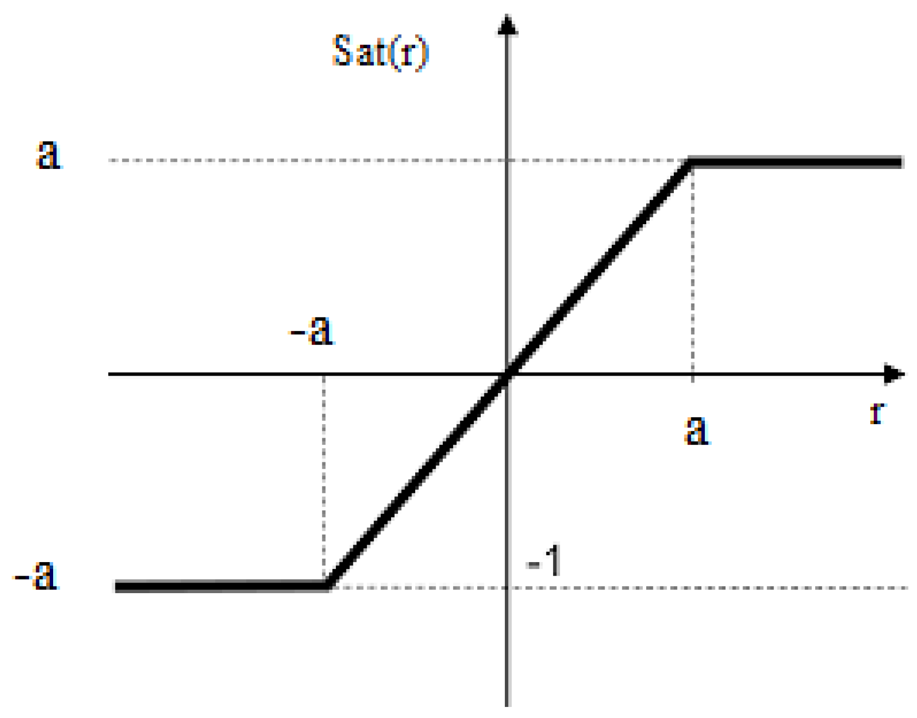
3.2. Saturation Control

In this section, we assume there is just the limitation of saturation on the controller, then (8) can be expressed as follows:

$$\left\{\begin{array}{c}{}^{C}D_t^v{i}_d=Sat\left(u_d\right)-\delta i_d+i_{q}w\hfill \\ {}^{C}D_t^v{i}_q=Sat(u_q/)-i_q-i_{d}w+\gamma w\hfill \\ {}^{C}D_t^{v}w=\sigma (i_q-w)-Sat\left(T_l\right)\hfill \end{array}\right.,0<v<1$$

(24)

In the presence of saturation control, stability analysis and design controller must be different. If we can introduce a group of controllers, it has a special condition. This section considers the system shown in Equation (24) and studies this special condition.

Theorem 4. 

Consider system (24) under assumptions (9)–(11). If there exist three positive numbers, $k_1,k_2$, and $k_3$, such that Equations (25) and (26) are satisfied, then the closed-loop system is globally exponentially stable at the zero equilibrium point:

$$p_1{i}_d{u}_d+(p_1-p_2)i_d{i}_{q}w+p_2{i}_q{u}_q+(p_2\gamma +p_3\sigma )w{i}_q-p_{3}w{T}_l\le 0$$

(25)

$$\begin{array}{c}{p}_1{i}_d(k_1+k_1^{-1}{A}^2)+(p_1-p_2)i_d{i}_{q}w+p_2{i}_q(k_2+k_2^{-1}{B}^2)+(p_2\gamma +p_3\sigma )w{i}_q\hfill \\ -p_{3}w(k_3+k_3^{-1}{C}^2)\le 0\hfill \end{array}$$

(26)

where $k_i$ and $p_i$, $i=1,2,3$ are positive scalars and $A,B,$ and C satisfy assumptions (9)–(11).

Proof. 

Based on Theorem 2, the system specified by Equation (24) can alternatively be expressed in another form as

$$\left\{\begin{array}{c}{\displaystyle \frac{\partial z_1\left(\omega ,t\right)}{\partial t}}=-\omega z_1(\omega ,t)+Sat\left(u_d\right)-\delta i_d+i_{q}w\hfill \\ i_d=\underset{0}{\overset{\infty }{\int }}{\mu }_v\left(\omega \right)z_1(\omega ,t)d\omega ,\hfill \\ {\mu }_v\left(\omega \right)={\displaystyle \frac{sin\left(v\pi \right)}{\pi {\omega }^v}}\hfill \end{array}\right.$$

(27)

$$\left\{\begin{array}{c}{\displaystyle \frac{\partial z_2\left(\omega ,t\right)}{\partial t}}=-\omega z_2(\omega ,t)+Sat\left(u_q\right)-i_q-i_{d}w+\gamma w\hfill \\ i_q=\underset{0}{\overset{\infty }{\int }}{\mu }_v\left(\omega \right)z_2(\omega ,t)d\omega ,\hfill \\ {\mu }_v\left(\omega \right)={\displaystyle \frac{sin\left(v\pi \right)}{\pi {\omega }^v}}\hfill \end{array}\right.$$

(28)

$$\left\{\begin{array}{c}{\displaystyle \frac{\partial z_3\left(\omega ,t\right)}{\partial t}}=-\omega z_3(\omega ,t)+\sigma (i_q-w)-Sat\left(T_l\right)\hfill \\ w=\underset{0}{\overset{\infty }{\int }}{\mu }_v\left(\omega \right)z_3(\omega ,t)d\omega ,\hfill \\ {\mu }_v\left(\omega \right)={\displaystyle \frac{sin\left(v\pi \right)}{\pi {\omega }^v}}\hfill \end{array}\right.$$

(29)

   □

Consider two Lyapunov functions. $V_1(\omega ,t)=p_1{z}_1^2+p_2{z}_2^2+p_3{z}_3^2$ is the monochromic Lyapunov function based on the elementary frequency, and the other Lyapunov function $V\left(t\right)$ is the sum of all the monochromatic $V_1\left(t\right)$s with the weight function ${\mu }_v\left(\omega \right)$:

$$V={\displaystyle \frac{1}{2}}\sum _{i=1}^3\underset{0}{\overset{\infty }{\int }}{\mu }_v\left(\omega \right)p_i{z}_i{(\omega ,t)}^{2}d\omega .$$

(30)

It can easily be derived from Equation (30) that

$${\displaystyle \frac{dV}{dt}}=\sum _{i=1}^3\underset{0}{\overset{\infty }{\int }}{\mu }_v\left(\omega \right)p_i{z}_i(\omega ,t){\displaystyle \frac{\partial z_i(\omega ,t)}{\partial t}}d\omega$$

(31)

Simplifying Equation (30),

$$\begin{array}{c}{\displaystyle \frac{dV}{dt}}=\underset{0}{\overset{\infty }{\int }}{\mu }_v\left(\omega \right)p_1{z}_1(\omega ,t){\displaystyle \frac{\partial z_1(\omega ,t)}{\partial t}}d\omega \hfill \\ +\underset{0}{\overset{\infty }{\int }}{\mu }_v\left(\omega \right)p_2{z}_2(\omega ,t){\displaystyle \frac{\partial z_2(\omega ,t)}{\partial t}}d\omega +\underset{0}{\overset{\infty }{\int }}{\mu }_v\left(\omega \right)p_3{z}_3(\omega ,t){\displaystyle \frac{\partial z_3(\omega ,t)}{\partial t}}d\omega \hfill \end{array}$$

(32)

Substituting Equations (27)–(29) into Equation (32), we have

$$\begin{array}{c}{\displaystyle \frac{dV}{dt}}=\underset{0}{\overset{\infty }{\int }}{\mu }_v\left(\omega \right)p_1{z}_1(\omega ,t)\left(-\omega z_1(\omega ,t)+Sat\left(u_d\right)-\delta i_d+i_{q}w\right)d\omega \hfill \\ +\underset{0}{\overset{\infty }{\int }}{\mu }_v\left(\omega \right)p_2{z}_2(\omega ,t)\left(-\omega z_2(\omega ,t)+Sat\left(u_q\right)-i_q-i_{d}w+\gamma w\right)d\omega \hfill \\ +\underset{0}{\overset{\infty }{\int }}{\mu }_v\left(\omega \right)p_3{z}_3(\omega ,t)\left(-\omega z_3(\omega ,t)+\sigma (i_q-w)-Sat\left(T_l\right)\right)d\omega \hfill \end{array}$$

(33)

This can be rewritten as

$$\begin{array}{c}{\displaystyle \frac{dV}{dt}}=\underset{0}{\overset{\infty }{\int }}-\omega {\mu }_v\left(\omega \right)\left\{p_1{z}_1^2(\omega ,t)+p_2{z}_2^2(\omega ,t)+p_3{z}_3^2(\omega ,t)\right\}d\omega \hfill \\ +\underset{0}{\overset{\infty }{\int }}{\mu }_v\left(\omega \right)p_1{z}_1(\omega ,t)d\omega \left(Sat\left(u_d\right)-\delta i_d+i_{q}w\right)\hfill \\ +\underset{0}{\overset{\infty }{\int }}{\mu }_v\left(\omega \right)p_2{z}_2(\omega ,t)d\omega \left(Sat\left(u_q\right)-i_q-i_{d}w+\gamma w\right)\hfill \\ +\underset{0}{\overset{\infty }{\int }}{\mu }_v\left(\omega \right)p_3{z}_3(\omega ,t)d\omega \left(\sigma (i_q-w)-Sat\left(T_l\right)\right)\hfill \end{array}$$

(34)

Simplifying Equation (34), we have

$$\begin{array}{c}{\displaystyle \frac{dV}{dt}}=\underset{0}{\overset{\infty }{\int }}-\omega {\mu }_v\left(\omega \right)\left\{p_1{z}_1^2(\omega ,t)+p_2{z}_2^2(\omega ,t)+p_3{z}_3^2(\omega ,t)\right\}d\omega \hfill \\ +p_1{i}_d\left(Sat\left(u_d\right)-\delta i_d+i_{q}w\right)+p_2{i}_q\left(Sat\left(u_q\right)-i_q-i_{d}w+\gamma w\right)\hfill \\ +p_{3}w\left(\sigma (i_q-w)-Sat\left(T_l\right)\right)\hfill \end{array}$$

(35)

Classifying Equation (35), it can be presented as

$$\begin{array}{c}{\displaystyle \frac{dV}{dt}}=\underset{0}{\overset{\infty }{\int }}-\omega {\mu }_v\left(\omega \right)\left\{p_1{z}_1^2(\omega ,t)+p_2{z}_2^2(\omega ,t)+p_3{z}_3^2(\omega ,t)\right\}d\omega \hfill \\ -\left\{p_1\delta i_d^2+p_2{i}_q^2+p_3\sigma w^2\right\}\hfill \\ +\left(p_1{i}_{d}Sat\left(u_d\right)+p_1{i}_d{i}_{q}w+p_2{i}_{q}Sat\left(u_q\right)-p_2{i}_q{i}_{d}w+p_2\gamma w{i}_q+p_{3}w\sigma i_q-p_{3}wSat\left(T_l\right)\right)\hfill \end{array}$$

(36)

The first and the second items of Equation (36) are negative definite since $\omega >0,{\mu }_{vi}>0$, and for the third term, we must consider two cases. The first case is when the saturation element is in the linear domain, $Sat\left(r\right)=r$, this means that there is no limitation on control; then the third term of Equation (36) can be rewritten as follows:

$$p_1{i}_d{u}_d+(p_1-p_2)i_d{i}_{q}w+p_2{i}_q{u}_q+(p_2\gamma +p_3\sigma )w{i}_q-p_{3}w{T}_l\le 0$$

(37)

If Equation (37) is negative, then the stability condition is satisfied in the linear case.

If there exists the limitation of saturation, then the third term of Equation (36) is as follows:

$$p_1{i}_{d}Sat\left(u_d\right)+(p_1-p_2)i_d{i}_{q}w+p_2{i}_{q}Sat\left(u_q\right)+(p_2\gamma +p_3\sigma )w{i}_q-p_{3}wSat\left(T_l\right)$$

(38)

Based on Lemma 1, we have

$$\begin{array}{c}{p}_1{i}_d(k_1+k_1^{-1}Sa{t}^2\left(u_d\right)+(p_1-p_2)i_d{i}_{q}w+p_2{i}_q(k_2+k_2^{-1}Sa{t}^2\left(u_q\right))\hfill \\ +(p_2\gamma +p_3\sigma )w{i}_q-p_{3}w(k_3+k_3^{-1}Sa{t}^2\left(T_l\right)\hfill \end{array}$$

(39)

Considering the three assumptions in Equations (9)–(11),

$$\begin{array}{c}{p}_1{i}_d(k_1+k_1^{-1}{A}^2)+(p_1-p_2)i_d{i}_{q}w+p_2{i}_q(k_2+k_2^{-1}{B}^2)\hfill \\ +(p_2\gamma +p_3\sigma )w{i}_q-p_{3}w(k_3+k_3^{-1}{C}^2)\le 0\hfill \end{array}$$

(40)

Equation (40) is negative until the stability condition holds. Thus, the proof is complete.

3.3. Rate Limitations

Rate limitation is a crucial aspect of control engineering, involving constraints on how quickly a system can change states or execute commands. Addressing rate limitations is essential for designing controllers that ensure stable and precise system responses. Research in this area is vital for improving control strategies and advancing control theory, leading to more adaptable systems in various real-world scenarios. Therefore, the study focuses on systems with up to two rate limitations as follows:

$$\left\{\begin{array}{c}{}^{C}D_t^v{i}_d=u_d-\delta i_d+i_{q}w,\parallel \dot{u_d}\parallel ⩽c_d\hfill \\ {}^{C}D_t^v{i}_q=u_q-i_q-i_{d}w+\gamma w,\parallel \dot{u_q}\parallel ⩽c_q\hfill \\ {}^{C}D_t^{v}w=\sigma (i_q-w)-T_l,\parallel \dot{T_l}\parallel ⩽c_T\hfill \end{array}\right.,0<v<1$$

(41)

where $c_d,c_q$, and $c_T$ are positive numbers that show rate limitation in specific inputs.

In the following, we present some theorems that consider the FOBLDCM system subject to rate limitations.

Theorem 5. 

The system described in Equation (41) can achieve global stability at the equilibrium point if the desired controller satisfies the following inequality:

$$\begin{array}{c}(i_d+c_{d}sgn\left({\dot{u}}_d\right))u_d+(i_q+c_{q}sgn\left({\dot{u}}_q\right))u_q+(\gamma +\sigma )w{i}_q-(w-c_{T}sgn\left({\dot{T}}_l\right))T_l\le 0.\hfill \end{array}$$

(42)

where $u_d$, $u_q$, and $T_l$ are the control inputs and $c_d$, $c_q$, and $c_T$ are, respectively, their rate limitations.

By substituting this controller into Equation (41) and satisfying the inequality constraint given by Equation (42), we can ensure the desired stability property.

Note 2. 

Note 1 is satisfied for Theorem 5.

Proof. 

We can alternatively consider a new Lyapunov candidate $V\left(t\right)$, which is defined as the sum of all the monochromatic functions $V_1\left(t\right)$ weighted by the function ${\mu }_v\left(\omega \right)$ and another functions as follows:

$$V={\displaystyle \frac{1}{2}}\sum _{i=1}^3\underset{0}{\overset{\infty }{\int }}{\mu }_v\left(\omega \right)z_i{(\omega ,t)}^{2}d\omega +{\displaystyle \frac{1}{2}}(u_q^2+u_d^2+T_l^2)$$

(43)

It can easily be derived from Equation (43) that

$${\displaystyle \frac{dV}{dt}}=\sum _{i=1}^3\underset{0}{\overset{\infty }{\int }}{\mu }_v\left(\omega \right)z_i(\omega ,t){\displaystyle \frac{\partial z_i(\omega ,t)}{\partial t}}d\omega +(\dot{u_q}{u}_q+\dot{u_d}{u}_d+\dot{T_l}{T}_l)$$

(44)

Simplifying Equation (44),

$$\begin{array}{c}{\displaystyle \frac{dV}{dt}}=\underset{0}{\overset{\infty }{\int }}{\mu }_v\left(\omega \right)z_1(\omega ,t){\displaystyle \frac{\partial z_1(\omega ,t)}{\partial t}}d\omega \hfill \\ +\underset{0}{\overset{\infty }{\int }}{\mu }_v\left(\omega \right)z_2(\omega ,t){\displaystyle \frac{\partial z_2(\omega ,t)}{\partial t}}d\omega +\underset{0}{\overset{\infty }{\int }}{\mu }_v\left(\omega \right)z_3(\omega ,t){\displaystyle \frac{\partial z_3(\omega ,t)}{\partial t}}d\omega \hfill \\ +{\dot{u}}_q{u}_q+{\dot{u}}_d{u}_d+{\dot{T}}_l{T}_l\hfill \end{array}$$

(45)

Substituting Equations (14)–(16) into Equation (45), we have

$$\begin{array}{c}{\displaystyle \frac{dV}{dt}}=\underset{0}{\overset{\infty }{\int }}{\mu }_v\left(\omega \right)z_1(\omega ,t)\left(-\omega z_1(\omega ,t)+u_d-\delta i_d+i_{q}w\right)d\omega \hfill \\ +\underset{0}{\overset{\infty }{\int }}{\mu }_v\left(\omega \right)z_2(\omega ,t)\left(-\omega z_2(\omega ,t)+u_q-i_q-i_{d}w+\gamma w\right)d\omega \hfill \\ +\underset{0}{\overset{\infty }{\int }}{\mu }_v\left(\omega \right)z_3(\omega ,t)\left(-\omega z_3(\omega ,t)+\sigma (i_q-w)-T_l\right)d\omega \hfill \\ +\dot{u_q}{u}_q+\dot{u_d}{u}_d+\dot{T_l}{T}_l\hfill \end{array}$$

(46)

Applying the rate limitation, we have

$$\begin{array}{c}{\displaystyle \frac{dV}{dt}}⩽\underset{0}{\overset{\infty }{\int }}-\omega {\mu }_v\left(\omega \right)\left\{z_1^2(\omega ,t)+z_2^2(\omega ,t)+z_3^2(\omega ,t)\right\}d\omega \hfill \\ +\underset{0}{\overset{\infty }{\int }}{\mu }_v\left(\omega \right)z_1(\omega ,t)d\omega \left(u_d-\delta i_d+i_{q}w\right)\hfill \\ +\underset{0}{\overset{\infty }{\int }}{\mu }_v\left(\omega \right)z_2(\omega ,t)d\omega \left(u_q-i_q-i_{d}w+\gamma w\right)\hfill \\ +\underset{0}{\overset{\infty }{\int }}{\mu }_v\left(\omega \right)z_3(\omega ,t)d\omega \left(\sigma (i_q-w)-T_l\right)\hfill \\ c_{q}sgn\left({\dot{u}}_q\right)u_q+c_{d}sgn\left({\dot{u}}_d\right)u_d+c_{T}sgn\left({\dot{T}}_l\right)T_l\hfill \end{array}$$

(47)

Simplifying Equation (47), we have

$$\begin{array}{c}{\displaystyle \frac{dV}{dt}}⩽\underset{0}{\overset{\infty }{\int }}-\omega {\mu }_v\left(\omega \right)\left\{z_1^2(\omega ,t)+z_2^2(\omega ,t)+z_3^2(\omega ,t)\right\}d\omega \hfill \\ +i_d\left(u_d-\delta i_d+i_{q}w\right)+i_q\left(u_q-i_q-i_{d}w+\gamma w\right)\hfill \\ +w\left(\sigma (i_q-w)-T_l\right)\hfill \\ c_{q}sgn\left({\dot{u}}_q\right)u_q+c_{d}sgn\left({\dot{u}}_d\right)u_d+c_{T}sgn\left({\dot{T}}_l\right)T_l\hfill \end{array}$$

(48)

Classifying Equation (48), it can be presented as

$$\begin{array}{c}{\displaystyle \frac{dV}{dt}}⩽\underset{0}{\overset{\infty }{\int }}-\omega {\mu }_v\left(\omega \right)\left\{z_1^2(\omega ,t)+z_2^2(\omega ,t)+z_3^2(\omega ,t)\right\}d\omega \hfill \\ -\left\{\delta i_d^2+i_q^2+\sigma w^2\right\}+\left\{\right((i_d+c_{d}sgn\left({\dot{u}}_d\right))u_d+\hfill \\ (i_q+c_{q}sgn\left({\dot{u}}_q\right))u_q+(\gamma +\sigma )w{i}_q-(w-c_{T}sgn\left({\dot{T}}_l\right))T_l\left)\right\}\hfill \end{array}$$

(49)

The first and second terms of (49) are negative definite due to $\omega \ge 0$, ${\mu }_{v_i}>0$, and ${\epsilon }_i>0$. The third term must be negative semi-definite to satisfy the stability condition ${\displaystyle \frac{dV}{dt}}<-\omega V$. Therefore, the true states will tend to zero and the FOBLDCM will be asymptotically stable. Thus, the proof is complete.    □

Corollary 1. 

The system described in Equation (41) can achieve global stability at the equilibrium point if there are three positive numbers, $k_1,k_2$, and $k_3$, and the following inequality is satisfied:

$$\begin{array}{c}(i_d+(k_1{c}_d^2+k_1^{-1}))u_d+(i_q+(k_2{c}_q^2+k_2^{-1}))u_q+(\gamma +\sigma )w{i}_q-(w-(k_3{c}_T^2+k_3^2))T_l\le 0\hfill \end{array}$$

(50)

where $u_d$, $u_q$, and $T_l$ are the control inputs and $c_d$, $c_q$, and $c_T$ are, respectively, their rate limitations.

Proof. 

The proof is similar to Theorem 5; the third term of Equation (49) based on Lemma 1 can be rewritten as

$$\begin{array}{c}(i_d+c_{d}sgn\left({\dot{u}}_d\right))u_d+(i_q+c_{q}sgn\left({\dot{u}}_q\right))u_q+(\gamma +\sigma )w{i}_q-(w-c_{T}sgn\left({\dot{T}}_l\right))T_l)=\hfill \\ (i_d+(k_1{c}_d^2+k_1^{-1}))u_d+(i_q+(k_2{c}_q^2+k_2^{-1}))u_q+(\gamma +\sigma )w{i}_q-(w-(k_3{c}_T^2+k_3^2))T_l\le 0\hfill \end{array}$$

(51)

The proof is completed.    □

3.4. Saturation and Rate Limitation Simultaneously

In this section, we consider saturation and rate limitations in the input control simultaneously. We conduct a stability analysis and derive the stability conditions under these limitations.

Theorem 6. 

Consider system (8) under assumptions (9)–(11). If there exist six positive numbers, $k_1,\dots k_6$, such that Equations (52) and (53) are satisfied simultaneously, then the closed-loop system is globally exponentially stable at the zero equilibrium point:

$$\begin{array}{c}(p_1{i}_d+c_{d}sgn\left({\dot{u}}_d\right))u_d+(p_1-p_2)i_d{i}_{q}w+(p_2{i}_q+c_{q}sgn\left({\dot{u}}_q\right))u_q+(p_2\gamma +p_3\sigma )w{i}_q\hfill \\ +(c_{T}sgn\left({\dot{T}}_l\right)-p_{3}w)T_l\le 0\hfill \end{array}$$

(52)

$$\begin{array}{c}{p}_1{i}_d(k_1+k_1^{-1}{A}^2)+(p_1-p_2)i_d{i}_{q}w+p_2{i}_q(k_2+k_2^{-1}{B}^2)+(p_2\gamma +p_3\sigma )w{i}_q\hfill \\ -p_{3}w(k_3+k_3^{-1}{C}^2)+c_q(k_4+k_4^{-1}{B}^2)+c_d(k_5+k_5^{-1}{A}^2)+c_T(k_5+k_6^{-1}{C}^2)\le 0\hfill \end{array}$$

(53)

where $k_i$ and $p_i$, $i=1,2,3$ are positive scalars and $A,B,$ and C satisfy assumptions (9)–(11).

Note 3. 

Note 1 is satisfied for this theorem.

Proof. 

Consider a Lyapunov function as follows:

$$V={\displaystyle \frac{1}{2}}\sum _{i=1}^3\underset{0}{\overset{\infty }{\int }}{\mu }_v\left(\omega \right)p_i{z}_i{(\omega ,t)}^{2}d\omega .+{\displaystyle \frac{1}{2}}(u_q^2+u_d^2+T_l^2)$$

(54)

It can easily be derived from Equation (54) that

$${\displaystyle \frac{dV}{dt}}=\sum _{i=1}^3\underset{0}{\overset{\infty }{\int }}{\mu }_v\left(\omega \right)p_i{z}_i(\omega ,t){\displaystyle \frac{\partial z_i(\omega ,t)}{\partial t}}d\omega +(\dot{u_q}{u}_q+\dot{u_d}{u}_d+\dot{T_l}{T}_l)$$

(55)

Simplifying Equation (55),

$$\begin{array}{c}{\displaystyle \frac{dV}{dt}}=\underset{0}{\overset{\infty }{\int }}{\mu }_v\left(\omega \right)p_1{z}_1(\omega ,t){\displaystyle \frac{\partial z_1(\omega ,t)}{\partial t}}d\omega +\underset{0}{\overset{\infty }{\int }}{\mu }_v\left(\omega \right)p_2{z}_2(\omega ,t){\displaystyle \frac{\partial z_2(\omega ,t)}{\partial t}}d\omega +\hfill \\ \underset{0}{\overset{\infty }{\int }}{\mu }_v\left(\omega \right)p_3{z}_3(\omega ,t){\displaystyle \frac{\partial z_3(\omega ,t)}{\partial t}}d\omega +(\dot{u_q}{u}_q+\dot{u_d}{u}_d+\dot{T_l}{T}_l)\hfill \end{array}$$

(56)

Substituting Equations (27)–(29) into Equation (56), we have

$$\begin{array}{c}{\displaystyle \frac{dV}{dt}}=\underset{0}{\overset{\infty }{\int }}{\mu }_v\left(\omega \right)p_1{z}_1(\omega ,t)\left(-\omega z_1(\omega ,t)+Sat\left(u_d\right)-\delta i_d+i_{q}w\right)d\omega \hfill \\ +\underset{0}{\overset{\infty }{\int }}{\mu }_v\left(\omega \right)p_2{z}_2(\omega ,t)\left(-\omega z_2(\omega ,t)+Sat\left(u_q\right)-i_q-i_{d}w+\gamma w\right)d\omega \hfill \\ +\underset{0}{\overset{\infty }{\int }}{\mu }_v\left(\omega \right)p_3{z}_3(\omega ,t)\left(-\omega z_3(\omega ,t)+\sigma (i_q-w)-Sat\left(T_l\right)\right)d\omega +(\dot{u_q}{u}_q+\dot{u_d}{u}_d+\dot{T_l}{T}_l)\hfill \end{array}$$

(57)

This can be rewritten as

$$\begin{array}{c}{\displaystyle \frac{dV}{dt}}=\underset{0}{\overset{\infty }{\int }}-\omega {\mu }_v\left(\omega \right)\left\{p_1{z}_1^2(\omega ,t)+p_2{z}_2^2(\omega ,t)+p_3{z}_3^2(\omega ,t)\right\}d\omega \hfill \\ +\underset{0}{\overset{\infty }{\int }}{\mu }_v\left(\omega \right)p_1{z}_1(\omega ,t)d\omega \left(Sat\left(u_d\right)-\delta i_d+i_{q}w\right)\hfill \\ +\underset{0}{\overset{\infty }{\int }}{\mu }_v\left(\omega \right)p_2{z}_2(\omega ,t)d\omega \left(Sat\left(u_q\right)-i_q-i_{d}w+\gamma w\right)\hfill \\ +\underset{0}{\overset{\infty }{\int }}{\mu }_v\left(\omega \right)p_3{z}_3(\omega ,t)d\omega \left(\sigma (i_q-w)-Sat\left(T_l\right)\right)+(\dot{u_q}{u}_q+\dot{u_d}{u}_d+\dot{T_l}{T}_l)\hfill \end{array}$$

(58)

Simplifying Equation (58), we have

$$\begin{array}{c}{\displaystyle \frac{dV}{dt}}=\underset{0}{\overset{\infty }{\int }}-\omega {\mu }_v\left(\omega \right)\left\{p_1{z}_1^2(\omega ,t)+p_2{z}_2^2(\omega ,t)+p_3{z}_3^2(\omega ,t)\right\}d\omega \hfill \\ +p_1{i}_d\left(Sat\left(u_d\right)-\delta i_d+i_{q}w\right)+p_2{i}_q\left(Sat\left(u_q\right)-i_q-i_{d}w+\gamma w\right)\hfill \\ +p_{3}w\left(\sigma (i_q-w)-Sat\left(T_l\right)\right)+(\dot{u_q}{u}_q+\dot{u_d}{u}_d+\dot{T_l}{T}_l)\hfill \end{array}$$

(59)

Classifying Equation (59) and applying the rate limitation, we have

$$\begin{array}{c}{\displaystyle \frac{dV}{dt}}=\underset{0}{\overset{\infty }{\int }}-\omega {\mu }_v\left(\omega \right)\left\{p_1{z}_1^2(\omega ,t)+p_2{z}_2^2(\omega ,t)+p_3{z}_3^2(\omega ,t)\right\}d\omega -\left\{p_1\delta i_d^2+p_2{i}_q^2+p_3\sigma w^2\right\}\hfill \\ +\left(p_1{i}_{d}Sat\left(u_d\right)+p_1{i}_d{i}_{q}w+p_2{i}_{q}Sat\left(u_q\right)-p_2{i}_q{i}_{d}w+p_2\gamma w{i}_q+p_{3}w\sigma i_q-p_{3}wSat\left(T_l\right)\right)+\hfill \\ c_{q}sgn\left({\dot{u}}_q\right)u_q+c_{d}sgn\left({\dot{u}}_d\right)u_d+c_{T}sgn\left({\dot{T}}_l\right)T_l\hfill \end{array}$$

(60)

Based on Lemma 1, we have three positive scalars, $k_1,k_2$, and $k_3$, that satisfy the following equation:

$$\begin{array}{c}{\displaystyle \frac{dV}{dt}}=\underset{0}{\overset{\infty }{\int }}-\omega {\mu }_v\left(\omega \right)\left\{p_1{z}_1^2(\omega ,t)+p_2{z}_2^2(\omega ,t)+p_3{z}_3^2(\omega ,t)\right\}d\omega -\left\{p_1\delta i_d^2+p_2{i}_q^2+p_3\sigma w^2\right\}\hfill \\ +\left(p_1{i}_{d}Sat\left(u_d\right)+p_1{i}_d{i}_{q}w+p_2{i}_{q}Sat\left(u_q\right)-p_2{i}_q{i}_{d}w+p_2\gamma w{i}_q+p_{3}w\sigma i_q-p_{3}wSat\left(T_l\right)\right)\hfill \\ (c_{q}sgn\left({\dot{u}}_q\right)u_q+c_{d}sgn\left({\dot{u}}_d\right)u_d+c_{T}sgn\left({\dot{T}}_l\right)T_l)\le 0\hfill \end{array}$$

(61)

The first and the second items of Equation (61) are negative definite since $\omega >0,{\mu }_{vi}>0$, and for the third term, we must consider two cases. The first case is when the saturation element is in the linear domain, $Sat\left(r\right)=r$, this means that there is no limitation on control; then the third term of Equation (61) can be rewritten as follows:

$$\begin{array}{c}(p_1{i}_d+c_{d}sgn\left({\dot{u}}_d\right))u_d+(p_1-p_2)i_d{i}_{q}w+(p_2{i}_q+c_{q}sgn\left({\dot{u}}_q\right))u_q+(p_2\gamma +p_3\sigma )w{i}_q+\hfill \\ (c_{T}sgn\left({\dot{T}}_l\right)-p_{3}w)T_l\le 0\hfill \end{array}$$

(62)

If Equation (62) is negative, then the stability condition is satisfied in the linear case.

If there exists the limitation of saturation, then the third and fourth terms of Equation (61) are as follows:

$$\begin{array}{c}{p}_1{i}_{d}Sat\left(u_d\right)+(p_1-p_2)i_d{i}_{q}w+p_2{i}_{q}Sat\left(u_q\right)+(p_2\gamma +p_3\sigma )w{i}_q-p_{3}wSat\left(T_l\right)+\hfill \\ (c_{q}sgn\left({\dot{u}}_q\right)u_q+c_{d}sgn\left({\dot{u}}_d\right)u_d+c_{T}sgn\left({\dot{T}}_l\right)T_l)\le 0\hfill \end{array}$$

(63)

In the worst case, when saturation control occurs, e.g., $u_d$ could not violate $Sat\left(u_d\right)$, then the above equation must be rewritten as

$$\begin{array}{c}{p}_1{i}_{d}Sat\left(u_d\right)+(p_1-p_2)i_d{i}_{q}w+p_2{i}_{q}Sat\left(u_q\right)+(p_2\gamma +p_3\sigma )w{i}_q-p_{3}wSat\left(T_l\right)+\hfill \\ (c_{q}sgn\left({\dot{u}}_q\right)Sat\left(u_q\right)+c_{d}sgn\left({\dot{u}}_d\right)Sat\left(u_d\right)+c_{T}sgn\left({\dot{T}}_l\right)Sat\left(T_l\right)\le 0\hfill \end{array}$$

(64)

Based on Lemma 1, we have

$$\begin{array}{c}{p}_1{i}_d(k_1+k_1^{-1}Sa{t}^2\left(u_d\right))+(p_1-p_2)i_d{i}_{q}w+p_2{i}_q(k_2+k_2^{-1}Sa{t}^2\left(u_q\right))\hfill \\ +(p_2\gamma +p_3\sigma )w{i}_q-p_{3}w(k_3+k_3^{-1}Sa{t}^2\left(T_l\right))+\hfill \\ c_q(k_4+k_4^{-1}Sa{t}^2\left(u_q\right))+c_d(k_5+k_5^{-1}Sa{t}^2\left(u_d\right))+c_T(k_5+k_6^{-1}Sa{t}^2\left(T_l\right))\le 0\hfill \end{array}$$

(65)

Considering the three assumptions of Equations (9)–(11),

$$\begin{array}{c}{p}_1{i}_d(k_1+k_1^{-1}{A}^2)+(p_1-p_2)i_d{i}_{q}w+p_2{i}_q(k_2+k_2^{-1}{B}^2)+(p_2\gamma +p_3\sigma )w{i}_q\hfill \\ -p_{3}w(k_3+k_3^{-1}{C}^2)+c_q(k_4+k_4^{-1}{B}^2)+c_d(k_5+k_5^{-1}{A}^2)+c_T(k_5+k_6^{-1}{C}^2)\le 0\hfill \end{array}$$

(66)

Equation (66) is negative until the stability condition holds. Thus, the proof is complete.    □

Corollary 2. 

Consider system (8) under assumptions (9)–(11). If there exist nine positive numbers, $k_1,\dots k_9$, such that Equations (67) and (68) are satisfied simultaneously, then the closed-loop system is globally exponentially stable at the zero equilibrium point:

$$\begin{array}{c}(p_1{i}_d+(k_7{c}_d^2+k_7^{-1}))u_d+(p_1-p_2)i_d{i}_{q}w+(p_2{i}_q+(k_8{c}_q^2+k_8^{-1}))u_q+\hfill \\ (p_2\gamma +p_3\sigma )w{i}_q+((k_9{c}_T^2+k_9^{-1})-p_{3}w)T_l\le 0\hfill \end{array}$$

(67)

$$\begin{array}{c}{p}_1{i}_d(k_1+k_1^{-1}{A}^2)+(p_1-p_2)i_d{i}_{q}w+p_2{i}_q(k_2+k_2^{-1}{B}^2)+(p_2\gamma +p_3\sigma )w{i}_q\hfill \\ -p_{3}w(k_3+k_3^{-1}{C}^2)+c_q(k_4+k_4^{-1}{B}^2)+c_d(k_5+k_5^{-1}{A}^2)+c_T(k_5+k_6^{-1}{C}^2)\le 0\hfill \end{array}$$

(68)

where $k_i$ and $p_i$, $i=1,2,3$ are positive scalars and $A,B,$ and C satisfy assumptions (9)–(11).

Note 4. 

Note 1 is satisfied for this theorem.

Proof. 

The proof is similar to Theorem 6 based on Lemma 1.    □

Note 5. 

In certain applications, it is crucial to utilize a single input. This is particularly relevant when contemplating the obtained theorems by adjusting a single input. We suggest employing straightforward controllers that involve only one state variable. This implies the need for just one sensor instead of the usual requirement of two or more in practical applications.

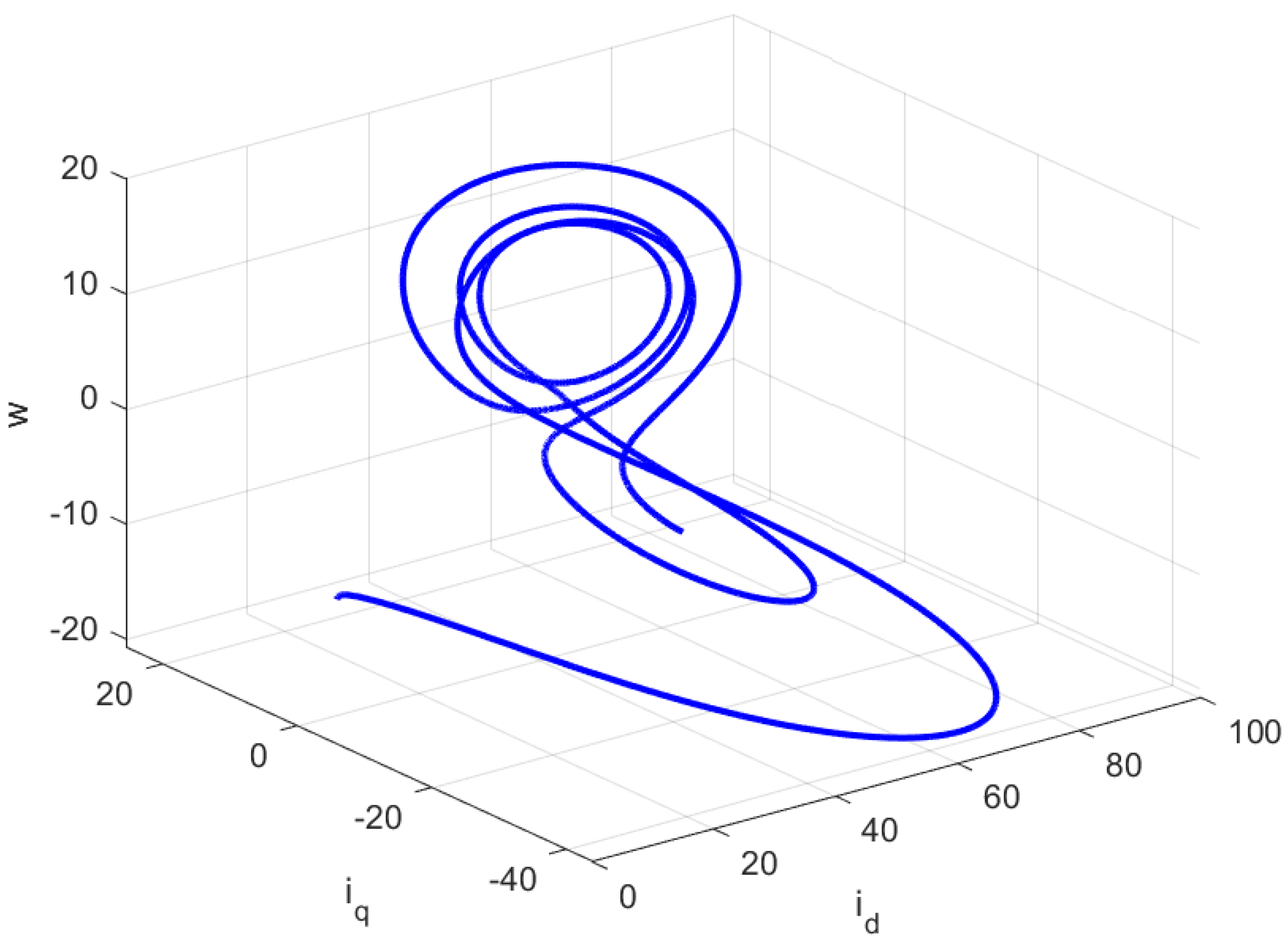
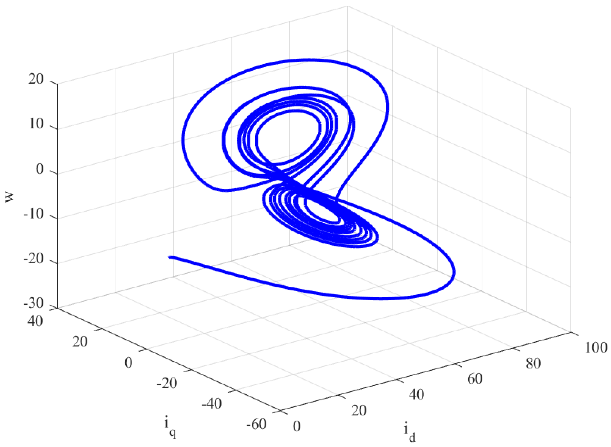
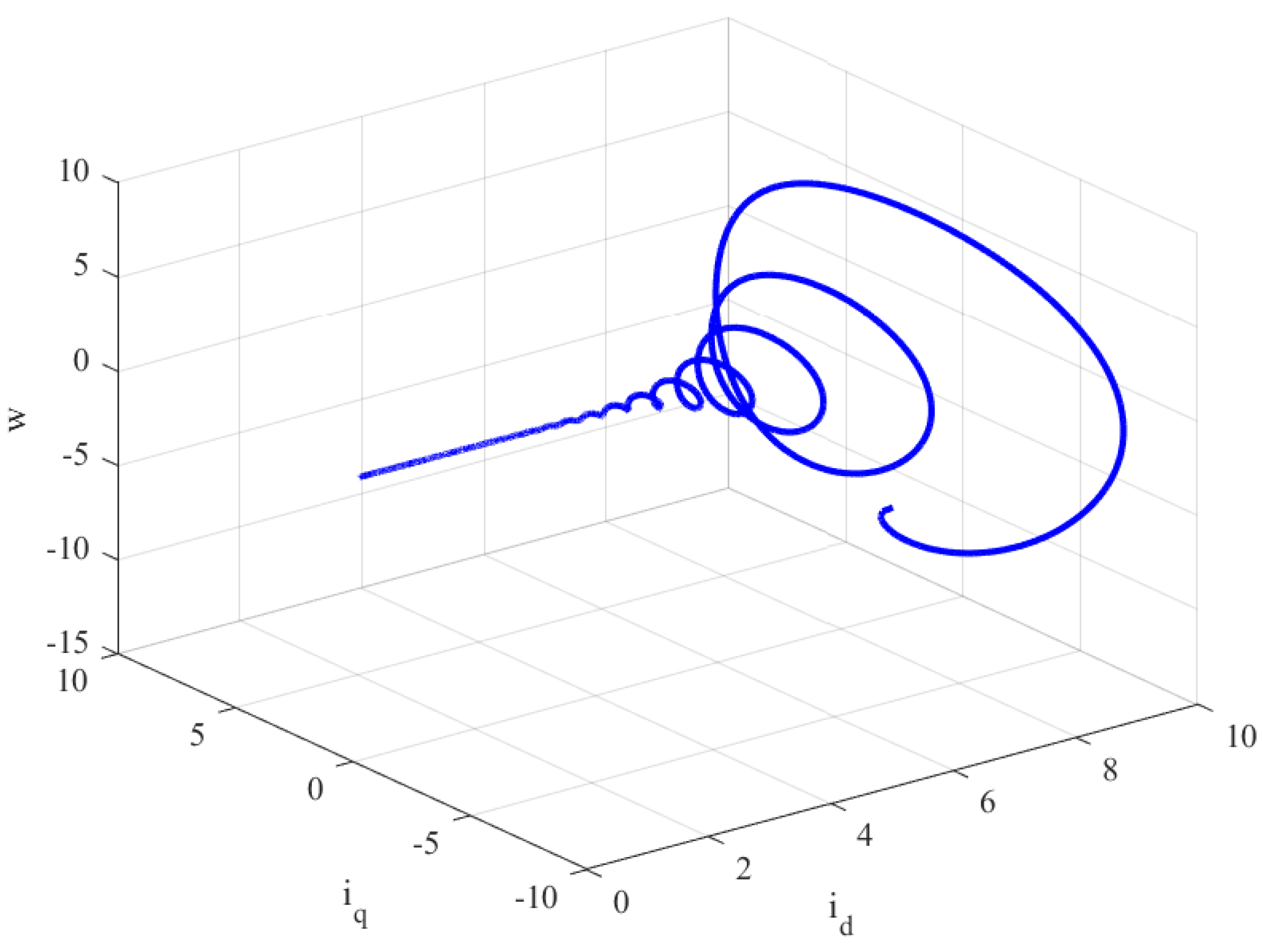
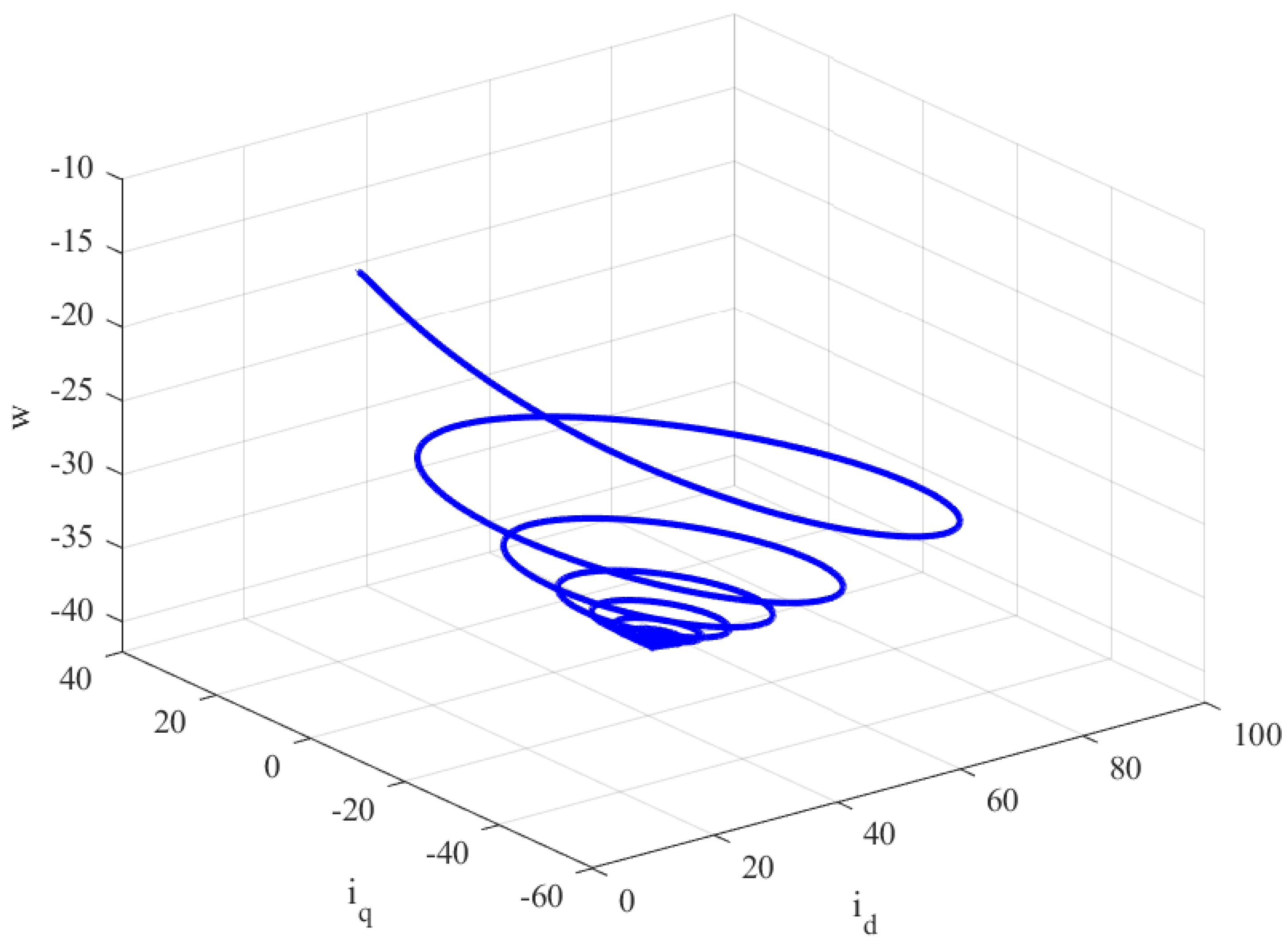
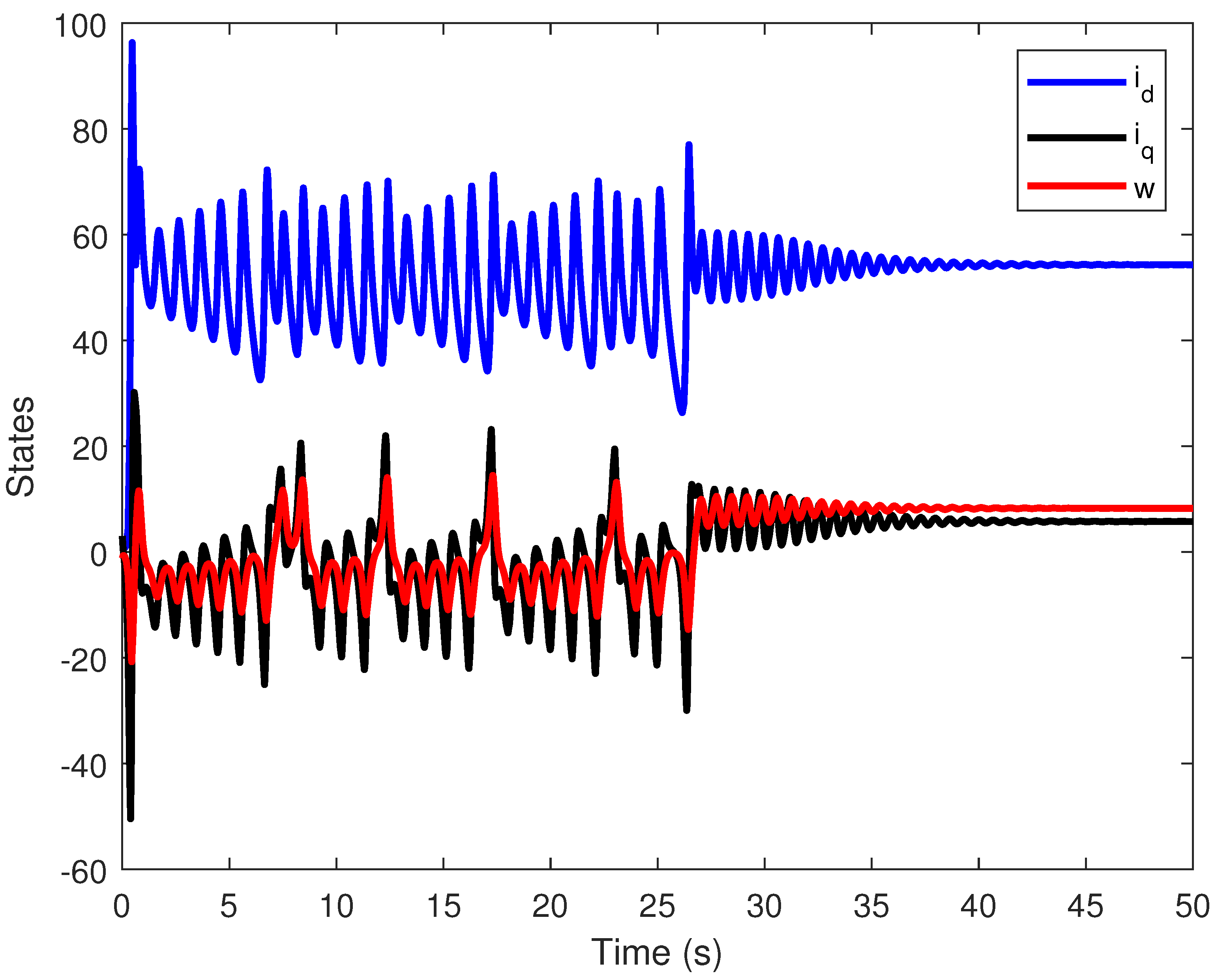
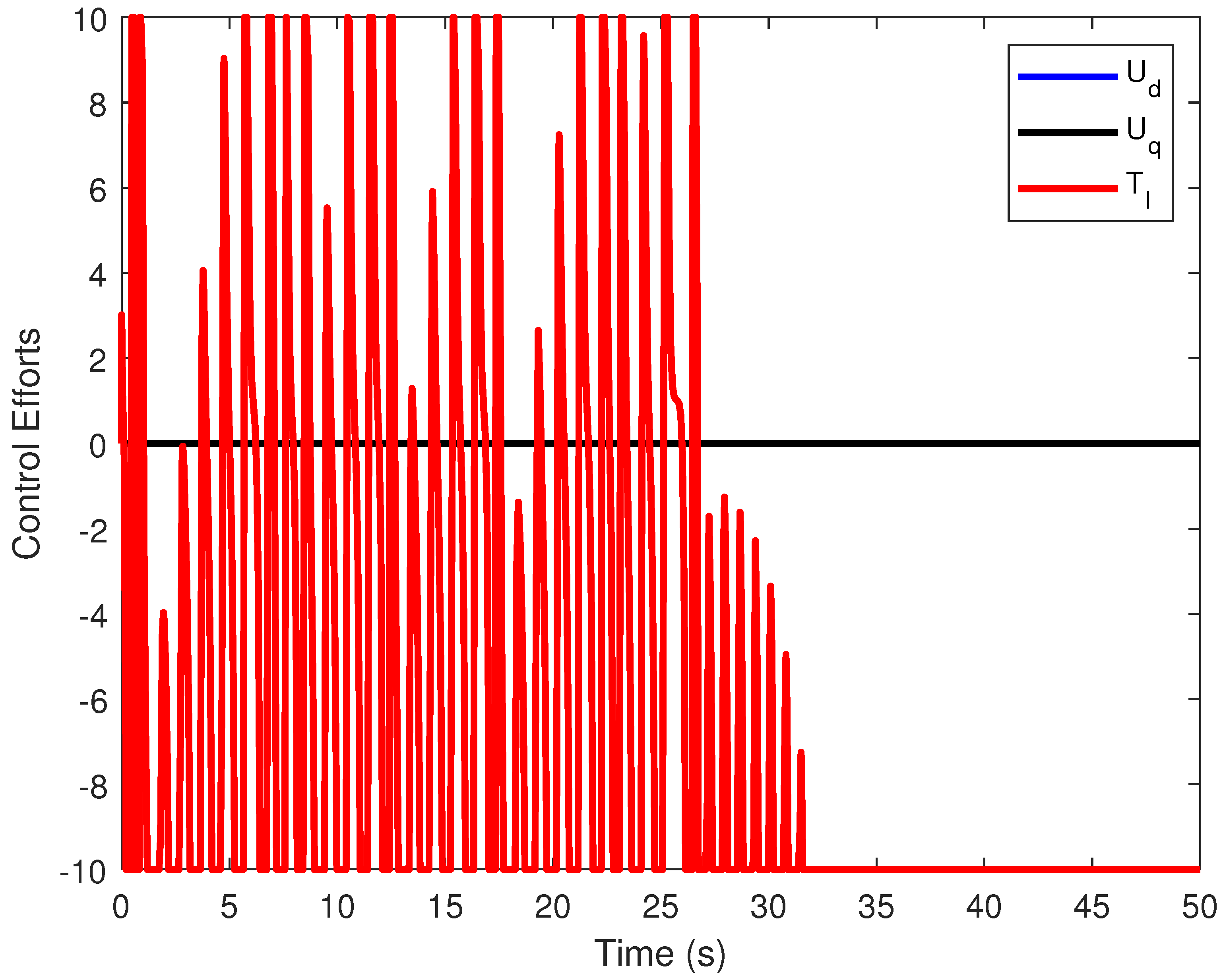
4. Numerical Simulations and Performance Evaluation

In this section, we first design a set of controllers that satisfy the stability conditions established by the theorems presented in this study, particularly those with single sufficient conditions, such as Theorems 3 and 5 in Section 3.1 and Section 3.3. These controllers are then validated through comprehensive numerical simulations conducted on the FOBLDCM model.

To assess the performance of the proposed control strategies, we employ the following quantitative criteria:

• Integral of squared error (ISE): Measures the accumulated squared tracking error over the simulation time for each state variable, reflecting the long-term tracking performance of the system.
• Root mean square error (RMSE): Evaluates the average deviation between the system outputs and their reference trajectories, providing a normalized metric for comparison.
• Control energy: Represents the total energy consumed by the control inputs, calculated as the integral of the squared control signal, and is used to evaluate the energy efficiency of the controller.
• Maximum control effort (${\mathit{u}}_{max}$): Denotes the peak value of the control input, serving as an indicator of actuator feasibility and the extent of input constraints such as saturation.

These criteria enable a fair and systematic comparison between different control approaches, particularly in the presence of input constraints. The numerical results for each case are presented and discussed in the following subsections.

After evaluating controllers designed based on single-condition theorems, we also propose and implement controllers that satisfy multi-condition theorems, such as those involving composite Lyapunov approaches.

Overall, the simulations are carried out across three general control scenarios:

• Scenario 1: Control without any actuator limitations;
• Scenario 2: Control with rate limitation constraint only;
• Scenario 3: Control under both saturation and rate limitation constraints simultaneously.

Scenario 1: Control Without Any Actuator Limitations

Table 1. Some desired controllers satisfying Theorem 3.

Input	Design Controller
Single Input	$\left\{\begin{array}{c}{u}_d=0\hfill \\ u_q=0\hfill \\ T_l=(\sigma +\gamma )i_q\hfill \end{array}\right.$	$\left\{\begin{array}{c}{u}_d=0\hfill \\ u_q=-(\sigma +\gamma )w\hfill \\ T_l=0\hfill \end{array}\right.$
Double Input	$\left\{\begin{array}{c}{u}_d=0\hfill \\ u_q=-\sigma w\hfill \\ T_l=\gamma i_q\hfill \end{array}\right.$	$\left\{\begin{array}{c}{u}_d=0\hfill \\ u_q=-\gamma w\hfill \\ T_l=\sigma i_q\hfill \end{array}\right.$
Triple Input	$\left\{\begin{array}{c}{u}_d=-i_q\hfill \\ u_q=i_d\hfill \\ T_l=(\gamma +\sigma )i_q\hfill \end{array}\right.$	$\left\{\begin{array}{c}{u}_d=i_q\hfill \\ u_q=-i_d\hfill \\ T_l=(\gamma +\sigma )i_q\hfill \end{array}\right.$
Triple Input	$\left\{\begin{array}{c}{u}_d=i_q\hfill \\ u_q=-(i_d+(\sigma +\gamma -1)w)\hfill \\ T_l=i_q\hfill \end{array}\right.$	$\left\{\begin{array}{c}{u}_d=w\hfill \\ u_q=w\hfill \\ T_l=i_d+(\gamma +\sigma +1)i_q\hfill \end{array}\right.$

presents a set of controllers based on Theorem 3. This set of controllers is designed without any constraints. We offer a range of controllers, including single-input, double-input, and triple-input controllers, tailored to meet different design requirements and conditions.

First Scenario: we consider the $\sigma =4$, we choose $v=0.97$ as the FO and an initial condition of ${\left[10,3,-12\right]}^T$. Based on the stability conditions derived from Theorem 3, the controller needs to satisfy the inequality $i_d{u}_d+i_q{u}_q+\gamma w{i}_q+w\sigma i_q-w{T}_l\le 0$ in the absence of limitations. One possible choice for the controller is $u_d=-i_q$, $u_q=i_d$, and $T_l=(\gamma +\sigma )i_q$. Figure 5 and Figure 6 illustrate the behavior of the closed-loop system and the phase plot of the FOBLDCM for the chosen FO $v=0.97$. It can be observed that after 4 s, the states of the FOBLDCM converge to the equilibrium point of the system. This demonstrates the effectiveness of the designed controller in achieving stability and graceful behavior of the FOBLDCM.

To benchmark the effectiveness of the proposed control framework, we perform a comparative analysis against an existing FOBLDCM control method reported in the literature. Specifically, the study in [39] addresses the stabilization of an FOBLDCM without considering any actuator constraints. The control law proposed in that work is $u_q=-80\omega$, which directly regulates the mechanical subsystem of the motor. Among the various controller configurations developed in the present work, the closest in structure to the method in [39] is given by $u_q=-(\sigma +\gamma )\omega =-59\omega$, highlighting a similar yet more energy-efficient approach.

To facilitate a fair and quantitative comparison, we evaluate several standard performance indices, including ISE, RMSE, control energy, and the maximum control input $u_{max}$. The results are summarized in

Table 2. Performance indices for comparison with Ref. [39].

Performance Indices	ISE	RMSE	Control Energy	${\mathit{u}}_{max}$
Controller from [39]	${\mathrm{ISE}}_{i_d}=76.063$ ${\mathrm{ISE}}_{i_q}=318.447$ ${\mathrm{ISE}}_w=76.063$	${\mathrm{RMSE}}_{i_d}=0.019$ ${\mathrm{RMSE}}_{i_q}=0.0064$ ${\mathrm{RMSE}}_w=0.0016$	$2.7153\times {10}^5$	$u_{i_q}=96$
Our proposed controller (close to [39])	${\mathrm{ISE}}_{i_d}=81.945$ ${\mathrm{ISE}}_{i_q}=291.604$ ${\mathrm{ISE}}_w=78.002$	${\mathrm{RMSE}}_{i_d}=0.0173$ ${\mathrm{RMSE}}_{i_q}=0.000229$ ${\mathrm{RMSE}}_w=0.0012$	$1.8321\times {10}^5$	$u_{i_q}=70.8$
Proposed controller Scenario 1	${\mathrm{ISE}}_{i_d}=66.685$ ${\mathrm{ISE}}_{i_q}=70.044$ ${\mathrm{ISE}}_w=78.953$	${\mathrm{RMSE}}_{i_d}=0.081$ ${\mathrm{RMSE}}_{i_q}=0.084$ ${\mathrm{RMSE}}_w=0.088$	$2.4383\times {10}^5$	$u_{i_d}=2.27$ $u_{i_q}=1$ $u_w=177$

. As shown, our proposed controller demonstrates superior performance in terms of lower control energy and reduced maximum control effort, while maintaining comparable or improved tracking accuracy across all state variables. These results underscore the practicality and robustness of the proposed controller under both constrained and unconstrained input scenarios.

Second scenario: In the second scenario, we consider the case where only rate limitations exist. Based on Theorem 5 and Note 2, we have $u_d=w$, $u_q=0$, and $T_l=c_d\mathrm{sgn}\left(\dot{w}\right)+i_d+(\gamma +\sigma )i_q$.

Implementing $c_T=0$, $c_q=10$, and $c_d=10$ in the proposed controller for the FOBLDCM yields encouraging outcomes, as evidenced by the convergence of the closed-loop system behaviors illustrated in Figure 7 and Figure 8 in the presence of rate limitations. The rapid stabilizing of the system, coupled with the manifestation of stability, underscores the efficacy and efficiency of the applied control strategy, aligning with the desired performance characteristics for practical applications.

Table 3. Some desired controllers satisfying Theorem 5.

Rate Limitation	Input	Design Controller
$c_T=0$ $c_q⩾0$ $c_d⩾0$	Single Input	$\left\{\begin{array}{c}{u}_d=0\hfill \\ u_q=0\hfill \\ T_l=(\sigma +\gamma )i_q\hfill \end{array}\right.$
	Double Input	$\left\{\begin{array}{c}{u}_d=w\hfill \\ u_q=0\hfill \\ T_l=c_{d}sgn\left(\dot{w}\right)+i_d+(\gamma +\sigma )i_q\hfill \end{array}\right.$
	Triple Input	$\left\{\begin{array}{c}{u}_d=w\hfill \\ u_q=w\hfill \\ T_l=(\gamma +\sigma +1)i_q+i_d+sgn\left(\dot{w}\right)(c_q+c_d)\hfill \end{array}\right.$
$c_q=0$ $c_d⩾0$ $c_T⩾0$	Single Input	$\left\{\begin{array}{c}{u}_d=0\hfill \\ T_l=0\hfill \\ u_q=-(\sigma +\gamma )w\hfill \end{array}\right.$
	Double Input	$\left\{\begin{array}{c}{u}_d=i_q\hfill \\ u_q=-(i_d+c_{d}sgn\left({\dot{i}}_q\right))-(\gamma +\sigma )w\hfill \\ T_l=0\hfill \end{array}\right.$
	Double Input	$\left\{\begin{array}{c}{u}_d=0\hfill \\ u_q=(w+c_{T}sgn\left({\dot{i}}_q\right))-(\gamma +\sigma )w\hfill \\ T_l=i_q\hfill \end{array}\right.$
	Triple Input	$\left\{\begin{array}{c}{u}_d=i_q\hfill \\ u_q=-i_d-(c_d+c_T)sgn\left({\dot{i}}_q\right)-(\gamma +\sigma -1)w\hfill \\ T_l=i_q\hfill \end{array}\right.$

presents several desired controllers that satisfy Theorem 5 and Note 1. This table also offers various controllers based on the available sensors or specific applications. It includes a new column labeled “rate limitation” where $c_d\ne 0$. It is essential to note that when $c_d=0$, Note 1 is not satisfied. This is because the polynomial $(\sigma +\gamma )i_{q}w$ lacks the presence of $i_d$. Consequently, for the designed controller, $i_d$ must appear in the denominator to meet the requirements of Note 1. Therefore, Note 1 is not satisfied in this case.

Third scenario: We consider both saturation and rate limitations in the input control. Under the previous conditions, the closed-loop system is unstable when saturation and rate limitations are applied to the input control. We assume that $A=B=C=10$ and the initial state is $(1,3,-1.2)$. By applying Theorem 6 and considering Corollary 2, we utilize the Matlab function Fmincon to achieve stability. We apply the control input as follows: $u_d=0$, $u_q=0$, and $T_l=-(\sigma +\gamma )u_{q}w/(c_T^2+1-w)+1$. This control input makes the closed-loop system asymptotically stable, and the states converge to zero. Figure 9 shows the time evolution of the state variables of the closed-loop system, while Figure 10 illustrates the input control. We deduce that the system can achieve stability even with saturation and rate limitations.

These improved and extended simulation results provide strong evidence of the effectiveness of the proposed control approaches for the FOBLDCM.

Table 4. Performance indices for third scenario.

Performance Indices	ISE	RMSE	Control Energy	${\mathit{u}}_{max}$
Proposed controller Scenario 3	${\mathrm{ISE}}_{i_d}=2.6524\times {10}^5$ ${\mathrm{ISE}}_{i_q}=1.075\times {10}^4$ ${\mathrm{ISE}}_w=4.2702\times {10}^4$	${\mathrm{RMSE}}_{i_d}=50.2996$ ${\mathrm{RMSE}}_{i_q}=1.9848$ ${\mathrm{RMSE}}_w=1.0439$	$6.63\times {10}^5$	$u_{i_d}=0$ $u_{i_q}=0$ $u_w=10$

presents the performance indices for the third control scenario, where both input saturation and rate limitation are simultaneously imposed. The proposed controller demonstrates satisfactory tracking performance under these challenging constraints. Specifically, the ISE for the direct-axis current ($i_d$), quadrature-axis current ($i_q$), and angular speed (w) is kept within acceptable bounds, with $IS{E}_{i_d}=2.65\times {10}^5$, $IS{E}_{i_q}=1.075\times {10}^4$, and $IS{E}_w=4.27\times {10}^4$, respectively. Furthermore, the RMSE indicates relatively smooth tracking with minimal steady-state deviation. The control energy remains moderate ($6.63\times {10}^5$), highlighting the controller’s efficiency in regulating the system without excessive actuation effort. Notably, the maximum control efforts ($u_{max}$) remain within the saturated limits—$u_{i_d}=0$, $u_{i_q}=0$, and $u_w=10$—demonstrating that the designed control law successfully respects both the amplitude and rate constraints while maintaining system stability and tracking accuracy.

Although the overall performance is not as favorable as in scenario 1, this decline is directly attributed to the presence of two stringent nonlinear constraints—saturation and rate limitation—imposed concurrently. Nevertheless, the results still validate the effectiveness and robustness of the proposed Lyapunov-based approach under severe practical limitations, reinforcing its applicability in real-world systems where such constraints are unavoidable.

Comparison with the results obtained in [34] demonstrates several key distinctions, as highlighted below:

• Proposed set of controllers based on available sensors: This paper introduces a comprehensive set of controllers tailored to the available sensors. In contrast, Ref. [34] proposed only a feedback linear controller, which can be considered a subset of the more general controller set presented in this work.
• Simultaneous consideration of saturation and rate limitation on the controller: This study addresses the FOBLDCM under the simultaneous constraints of saturation and rate limitation on the controller. In comparison, Ref. [34] only considered saturation as a limitation without accounting for rate limitation. Furthermore, other valuable papers did not consider any constraints [17,18,19,23,24,39].
• Robust solution approach: The proposed results in this paper are derived using a presented novel Lyapunov candidate to establish novel stability conditions in the presence of rate limitations and saturated control inputs. On the other hand, Ref. [34] relied on estimations of the solutions to the given equations, which presents a less robust approach than the one presented in this paper.

Table 5. Comparison of proposed work with related studies.

Feature	Proposed Work	[34]	[39]
Controller design based on sensor availability	Comprehensive set (single/double/triple input)	Only feedback linearization	Only feedback linearization
Constraints considered	Both saturation and rate limitation	Only saturation	No constraints
Stability analysis method	Lyapunov-based analytical approach	Estimation-based	Estimation-based
Robustness	High (based on derived sufficient conditions)	Moderate lack of rate-limit handling	Moderate lack of saturation and rate-limit handling

summarizes the above statements.

The achieved stability, convergence, and desired system behavior highlight the practical applicability and potential of the proposed methods in real-world applications. These findings contribute to the advancement of control techniques for FOBLDCMs, opening up new possibilities for their utilization in various domains.

5. Conclusions

This work addresses the stabilization problem of fractional-order chaotic brushless DC motors (FOBLDCMs) subject to input constraints, including saturation and rate limits, within the fractional domain $0<v<1$. The proposed approach overcomes the limitations of classical methods by developing a unified framework that explicitly incorporates actuator constraints into the control design process. The primary contributions of this research can be summarized as follows:

• Novel Lyapunov candidates: Dedicated Lyapunov functions are constructed for each control scenario—namely, unconstrained, saturated, rate-limited, and jointly constrained—by integrating both direct and indirect Lyapunov-based techniques tailored to fractional-order dynamics.
• Input-constrained controller design: Multiple controller configurations are derived based on the developed stability conditions, enabling practical implementation with reduced sensor dependencies through single-input, double-input, and triple-input controller variants. To the best of our knowledge, this is the first study to simultaneously address both amplitude and rate constraints in the control design of FO chaotic systems.
• Benchmark validation: The effectiveness of the proposed framework is validated through extensive numerical simulations conducted on FO chaotic BLDCMs under varying degrees of nonlinear behavior and input limitations, providing a solid benchmark for future studies.

Practical significance: The proposed framework is particularly beneficial for precision motion control applications where BLDC motors are subjected to strict actuator limitations—common in electric vehicles, robotic manipulators, unmanned aerial vehicles (UAVs), and industrial automation. By explicitly considering actuator constraints, the designed controllers prevent performance degradation, avoid instability caused by saturation-induced limit cycles, and ensure safe motor operation, especially in embedded and energy-limited platforms.

Technological recommendations:

-

For manufacturers: It is recommended to embed FO control logic and constraint-aware algorithms within motor control chips or firmware, enabling higher-fidelity performance in FO dynamic environments. Support for configurable constraint-aware control modules should be considered during motor drive design.

-

For system integrators and end users: When selecting control algorithms for high-precision or safety-critical systems, priority should be given to those that explicitly handle rate and amplitude constraints. The use of adaptable multi-input controllers can provide significant performance benefits when sensor configurations are flexible.

In conclusion, this study offers a scalable, constraint-aware control strategy for a class of nonlinear FO systems, addressing both theoretical and practical challenges. Future work will focus on real implementation, robustness under parametric uncertainty, and experimental validation on physical motor platforms.

References

- Fu, H.; Wu, G.C.; Yang, G.; Huang, L.L. Fractional calculus with exponential memory. Chaos Interdiscip. J. Nonlinear Sci. 2021, 31, 031103. [Google Scholar] [CrossRef] [PubMed]
- Wang, S.; Zhang, S. The global classical solution to compressible system with fractional viscous term. Nonlinear Anal. Real World Appl. 2024, 75, 103963. [Google Scholar] [CrossRef]
- Jiang, K.; Liu, Z.; Zhou, L. Global existence and asymptotic dynamics in a 3D fractional chemotaxis system with singular sensitivity. Nonlinear Anal. Real World Appl. 2020, 54, 103103. [Google Scholar] [CrossRef]
- Luo, H.; Tang, X. Ground state and multiple solutions for the fractional Schrödinger–Poisson system with critical Sobolev exponent. Nonlinear Anal. Real World Appl. 2018, 42, 24–52. [Google Scholar] [CrossRef]
- Zhang, Y.; Li, J.; Zhu, S.; Zhao, H. Bifurcation and chaos detection of a fractional Duffingvan der Pol oscillator with two periodic excitations and distributed time delay. Chaos Interdiscip. J. Nonlinear Sci. 2023, 33, 083153. [Google Scholar] [CrossRef]
- Tian, Q.; Yang, X.; Zhang, H.; Xu, D. An implicit robust numerical scheme with graded meshes for the modified Burgers model with nonlocal dynamic properties. Comput. Appl. Math. 2023, 42, 246. [Google Scholar] [CrossRef]
- Alaviyan Shahri, E.S.; Alfi, A.; Tenreiro Machado, J.A. Robust stability and stabilization of uncertain fractional order systems subject to input saturation. J. Vib. Control. 2018, 24, 3676–3683. [Google Scholar] [CrossRef]
- Chen, L.; Huang, C.; Liu, H.; Xia, Y. Anti-synchronization of a class of chaotic systems with application to Lorenz system: A unified analysis of the integer order and fractional order. Mathematics 2019, 7, 559. [Google Scholar] [CrossRef]
- Li, C.; Chen, G. Chaos in the fractional order Chen system and its control. Chaos Solitons Fractals 2004, 22, 549–554. [Google Scholar] [CrossRef]
- Lu, J.G. Chaotic dynamics of the fractional-order Lü system and its synchronization. Phys. Lett. A 2006, 354, 305–311. [Google Scholar] [CrossRef]
- Rajagopal, K.; Vaidyanathan, S.; Karthikeyan, A.; Duraisamy, P. Dynamic analysis and chaos suppression in a fractional order brushless DC motor. Electr. Eng. 2017, 99, 721–733. [Google Scholar] [CrossRef]
- Hemati, N. Strange attractors in brushless DC motors. IEEE Trans. Circuits Syst. Fundam. Theory Appl. 1994, 41, 40–45. [Google Scholar] [CrossRef]
- Liu, D.; Zhou, G.; Liao, X. Global exponential stabilization for chaotic brushless DC motor with simpler controllers. Trans. Inst. Meas. Control. 2019, 41, 2678–2684. [Google Scholar] [CrossRef]
- Faradja, P.; Qi, G. Analysis of multistability, hidden chaos and transient chaos in brushless DC motor. Chaos Solitons Fractals 2020, 132, 109606. [Google Scholar] [CrossRef]
- Bi, H.; Qi, G.; Hu, J. Modeling and analysis of chaos and bifurcations for the attitude system of a quadrotor unmanned aerial vehicle. Complexity 2019, 2019, 6313925. [Google Scholar] [CrossRef]
- Kingni, S.T.; Cheukem, A.; Tsafack, A.S.; Kengne, R.; Mboupda Pone, J.R.; Wei, Z. Spiking oscillations and multistability in nonsmoothairgap brushless direct current motor: Analysis, circuit validation and chaos control. Int. Trans. Electr. Energy Syst. 2021, 31, 12575. [Google Scholar]
- Zhou, P.; Cai, H.; Yang, C. Stabilization of the unstable equilibrium points of the fractional-order BLDCM chaotic system in the sense of Lyapunov by a single-state variable. Nonlinear Dyn. 2016, 84, 2357–2361. [Google Scholar] [CrossRef]
- Zafar, Z.U.A.; Ali, N.; Tunc, C. Mathematical modelling and analysis of fractional-order brushless DC motor. Adv. Differ. Equations 2021, 2021, 433. [Google Scholar] [CrossRef]
- Mohammadzadeh, A.; Ahmadian, A.; Elkamel, A.; Alhameli, F. Chaos synchronization of brushes direct current motors for electric vehicle: Adaptive fuzzy immersion and invariance approach. Trans. Inst. Meas. Control. 2021, 43, 178–193. [Google Scholar] [CrossRef]
- Abro, K.A.; Atangana, A.; Gómez-Aguilar, J.F. Chaos control and characterization of brushless DC motor via integral and differential fractal-fractional techniques. Int. J. Model. Simul. 2023, 43, 416–425. [Google Scholar] [CrossRef]
- Zhang, H.; Wu, H.; Jin, H.; Li, H. High-dynamic and low-cost sensorless control method of high-speed brushless DC motor. IEEE Trans. Ind. Inform. 2022, 19, 5576–5584. [Google Scholar] [CrossRef]
- Souhail, W.; Khammari, H. Sensorless anti-control and synchronization of chaos of brushless DC motor driver. Sci. Rep. 2025, 15, 13899. [Google Scholar] [CrossRef] [PubMed]
- Zhou, P.; Bai, R.J.; Zheng, J.M. Stabilization of a fractional-order chaotic brushless DC motor via a single input. Nonlinear Dyn. 2015, 82, 519–525. [Google Scholar] [CrossRef]
- Zhong, X.; Shahidehpour, M.; Zou, Y. Global quasi-Mittag-Leffler stability of distributed-order BLDCM system. Nonlinear Dyn. 2022, 108, 2405–2416. [Google Scholar] [CrossRef]
- Yu, Z.; Sun, Y.; Dai, X. Stability and stabilization of the fractional-order power system with time delay. IEEE Trans. Circuits Syst. II Express Briefs 2021, 68, 3446–3450. [Google Scholar] [CrossRef]
- Mok, R.; Ahmad, M.A. Smoothed functional algorithm with norm-limited update vector for identification of continuous-time fractional-order Hammerstein models. IETE J. Res. 2024, 70, 1814–1832. [Google Scholar] [CrossRef]
- Wang, J.; Ji, Y.; Ding, F. Iterative parameter estimation for a class of fractional-order Hammerstein nonlinear systems disturbed by colored noise. Proc. Inst. Mech. Eng. Part I J. Syst. Control. Eng. 2025. [Google Scholar] [CrossRef]
- Alsaadi, F.E.; Jahanshahi, H.; Yao, Q.; Mou, J. Recurrent neural network-based technique for synchronization of fractional-order systems subject to control input limitations and faults. Chaos Solitons Fractals 2023, 173, 113717. [Google Scholar] [CrossRef]
- Yuan, J.; Fei, S.; Chen, Y.; Ding, Y. Robust feedback compensation and PID Tuning under actuator rate limit effect based on Bode s integrals. Control. Eng. Pract. 2022, 129, 105347. [Google Scholar] [CrossRef]
- Wu, Z.; Yuan, J.; Liu, Y.; Li, D.; Chen, Y. An active disturbance rejection control design with actuator rate limit compensation for the ALSTOM gasifier benchmark problem. Energy 2021, 227, 120447. [Google Scholar] [CrossRef]
- Alaviyan Shahri, E.S.; Balochian, S. An analysis and design method for fractional order linear systems subject to actuator saturation and disturbance. Optim. Control. Appl. Methods 2016, 37, 305–322. [Google Scholar] [CrossRef]
- Shahri, E.S.A.; Balochian, S. Stability region for fractional-order linear system with saturating control. J. Control. Autom. Electr. Syst. 2014, 25, 283–290. [Google Scholar] [CrossRef]
- Alaviyan Shahri, E.S.; Balochian, S. A stability analysis on fractional order linear system with nonlinear saturated disturbance. Natl. Acad. Sci. Lett. 2015, 38, 409–413. [Google Scholar] [CrossRef]
- Alaviyan Shahri, E.S.; Alfi, A.; Tenreiro Machado, J.A. Stability analysis of a class of nonlinear fractional order systems under control input saturation. Int. J. Robust Nonlinear Control. 2018, 28, 2887–2905. [Google Scholar] [CrossRef]
- Alaviyan Shahri, E.S.; Pariz, N.; Chen, Y. Stabilization of a Class of Fractional-Order Nonlinear Systems Subject to Actuator Saturation and Time Delay. Appl. Sci. 2025, 15, 1851. [Google Scholar] [CrossRef]
- Chen, Y.; Wei, Y.; Zhou, X.; Wang, Y. Stability for nonlinear fractional order systems: An indirect approach. Nonlinear Dyn. 2017, 89, 1011–1018. [Google Scholar] [CrossRef]
- Wang, B.; Ding, J.; Wu, F.; Zhu, D. Robust finite-time control of fractional-order nonlinear systems via frequency distributed model. Nonlinear Dyn. 2016, 85, 2133–2142. [Google Scholar] [CrossRef]
- Tan, Y.; Xiong, M.; Du, D.; Fei, S. Observer-based robust control for fractional-order nonlinear uncertain systems with input saturation and measurement quantization. Nonlinear Anal. Hybrid Syst. 2019, 34, 45–57. [Google Scholar] [CrossRef]
- Huang, S.; Wang, B. Stabilization of a fractional-order nonlinear brushless direct current motor. J. Comput. Nonlinear Dyn. 2017, 12, 041005. [Google Scholar] [CrossRef]