The Optimal L²-Norm Error Estimate of a Weak Galerkin Finite Element Method for a Multi-Dimensional Evolution Equation with a Weakly Singular Kernel

Abstract

This paper proposes a weak Galerkin (WG) finite element method for solving a multi-dimensional evolution equation with a weakly singular kernel. The temporal discretization employs the backward Euler scheme, while the fractional integral term is approximated via a piecewise constant function method. A fully discrete scheme is constructed by integrating the WG finite element approach for spatial discretization. $L^2$-norm stability and convergence analysis of the fully discrete scheme are rigorously established. Numerical experiments are conducted to validate the theoretical findings and demonstrate optimal convergence order in both spatial and temporal directions. The numerical results confirm that the proposed method achieves an accuracy of the order $O\left(\tau +h^{k+1}\right)$, where $\tau$ and h represent the time step and spatial mesh size, respectively. This work extends previous studies on one-dimensional problems to higher spatial dimensions, providing a robust framework for handling evolution equations with a weakly singular kernel.

1. Introduction

In recent years, fractional calculus has gained substantial prominence due to its critical role in modeling complex physical and engineering phenomena such as viscoelasticity, anomalous diffusion, and fluid dynamics [1,2]. This study focuses on the numerical solution of a multi-dimensional evolution equation with a weakly singular kernel which can be found in applications to the above different fields, especially concerning multidimensional problems of such equations. Specifically, we consider the initial boundary value problem [3,4,5,6,7]:

$$u_t(\mathbf{x},t)-{\displaystyle \frac{1}{\Gamma \left(\alpha \right)}}{\int }_0^t{(t-s)}^{\alpha -1}\Delta u(\mathbf{x},s)ds=f(\mathbf{x},t),\mathbf{x}\in \Omega ,t\in (0,T],$$

(1)

for $0<\alpha <1$, with the initial condition

$$u(\mathbf{x},0)=\psi \left(\mathbf{x}\right),\mathbf{x}\in \Omega ,$$

(2)

and the boundary condition

$$u(\mathbf{x},t)=0,\mathbf{x}\in \partial \Omega ,0<t\le T,$$

(3)

where $\Omega$ is an open bounded domain in ${\mathbb{R}}^d(d=2,3)$, and $\psi \left(\mathbf{x}\right)$ and $f(\mathbf{x},t)$ are given smooth functions.

Numerous numerical strategies have been proposed for such Equations (1)–(3). Early contributions include finite difference schemes by Chen and Xu [3], who analyzed stability and convergence, and piecewise linear finite element methods combined with backward Euler temporal discretization by Chen and Thomée [4], who established rigorous error estimates. In [5], Mclean and Thomée employed the finite difference method in time and Galerkin finite element method in space for equations and gave regularity, stability, and error estimates. Also, we can find other methods for evolution equations with a weakly singular kernel such as the compact finite difference method [6,7], spectral method [8], discontinuous Galerkin finite element method [9], finite volume method [10], two-grid algorithm [11], Sinc collocation method [12], and orthogonal spline collocation method [13,14], each addressing specific challenges in accuracy or computational efficiency. In these studies, scholars have systematically developed corresponding numerical solution schemes for the equations, performed rigorous theoretical analyses and numerical computations of the schemes, and provided numerical examples for verification. There are also other computational techniques [15,16] for studying and calculating evolution equations. Despite these developments, extending these methods to multi-dimensional settings while maintaining optimal convergence rates remains nontrivial, particularly for problems involving weakly singular kernels.

Recently, the WG finite element method has attracted much attention in the numerical calculation community; this method was first introduced in [17] by Wang and Ye for the second-order elliptic problem. It is an extension of the standard Galerkin finite element method, and the difference between them is that the classical derivatives are replaced by weakly defined derivatives on functions with discontinuity. More information on differences between this method and other finite element methods can be found in the article [18]. Since then, the WG finite element method had been extensive applied for solving PDEs [19,20,21,22,23,24,25].

Regarding research related to this problem, our existing research was published in [26,27,28]. In [26], we presented the WG finite element scheme for one-dimensional parabolic integro-differential equations with a weakly singular kernel and gave the stability and convergence of the scheme. In [27], we employed the finite difference method in time and the WG finite element method in space for the multi-term time-fractional diffusion equation and gave the stability and error estimates. Finally, numerical examples were given to verify the correctness of the theory. In [28], the WG finite element method was used for the time-fractional quasi-linear diffusion equation with a Caputo time derivative. The Caputo time derivative was discretized by the $L^1$ method and the Newton linear method was used for the quasi-linear term with graded meshes in the time direction. These existing studies have all performed sufficient preparatory theoretical and computational work for our current research.

In our prior work [26], the WG finite element method demonstrated efficacy for one-dimensional parabolic integro-differential equations with a weakly singular kernel. However, its application in multi-dimensional evolution equations has not been explored, and systematic research is needed on stability, convergence, and computational feasibility. This paper bridges this gap by constructing a fully discrete scheme for multi-dimensional evolution equations which combines the WG finite element method in space with backward Euler temporal discretization and a piecewise constant approximation for the fractional integral term.

Our contributions in this work are summarized as follows.

• A WG finite element fully discrete scheme is constructed for a multi-dimensional evolution equation with a weakly singular kernel.
• The stability and convergence of the discrete approximation are proved.

This paper is organized as follows. In Section 2, the WG finite element method is introduced and the fully discrete scheme is presented. In Section 3 and Section 4, we analyze stability and convergence of the fully discrete scheme. In Section 5, some numerical experiments to verify our analysis are given.

Throughout this paper, we cite the usual Sobolev space; the notation $H^s(\Omega )$ means the norm ${\parallel ·\parallel }_s={\parallel ·\parallel }_{H^s(\Omega )}$ on $\Omega$. We denote the $L^2(\Omega )$-inner product and $L^2(\Omega )$-norms by $(·,·)$ and $\parallel ·\parallel$, respectively. The letter C, which denotes a positive constant independent of $\tau$ and h, represents different values in different appearances.

2. Weak Galerkin Finite Element Scheme

Let ${\mathcal{T}}_h=\bigcup \left\{\mathcal{T}\right\}$ denote a shape-regular mesh partitioning the domain $\Omega \subset {\mathbb{R}}^d$. In two dimensions, we consider triangular or rectangular meshes, and in three dimensions, we mainly consider tetrahedral and hexahedral meshes. We set the mesh size $h={max}_{\mathcal{T}\in {\mathcal{T}}_h}{h}_{\mathcal{T}}$, where $h_{\mathcal{T}}$ is the diameter of the element $\mathcal{T}$. The union of all elements is denoted by $\overline{\Omega }={\bigcup }_{\mathcal{T}\in {\mathcal{T}}_h}\mathcal{T}$. For each element $\mathcal{T}\in {\mathcal{T}}_h$ with the boundary $\partial \mathcal{T}$, let $\left|\mathcal{T}\right|$ represent its area and $\left|e\right|$ denote the length of an edge, e. A weak function, $v=\{v_0,v_b\}$, is defined on $\mathcal{T}$ such that $v_0\in L^2\left(\mathcal{T}\right)$ represents the value of v in T and $v_b\in L^2(\partial \mathcal{T})$ represents the the value of v on $\partial \mathcal{T}$, which is not necessarily the trace of $v_0$ on $\partial \mathcal{T}$.

The space of weak functions on $\mathcal{T}$ is defined as

$$W\left(\mathcal{T}\right)=\left\{v=\{v_0,v_b\}|v_0\in L^2\left(\mathcal{T}\right),v_b\in L^2(\partial \mathcal{T})\right\}.$$

For each element $\mathcal{T}\in {\mathcal{T}}_h$, the local polynomial weak function space is given by

$$W(\mathcal{T},k,l)=\left\{v=\{v_0,v_b\}|v_0{{|}_{{\mathcal{T}}^0}\in P_k\left({\mathcal{T}}^0\right),v_b|}_{\partial \mathcal{T}}\in P_l(\partial \mathcal{T})\right\},$$

where ${\mathcal{T}}^0$ and $\partial \mathcal{T}$ denote the interior and boundary of $\mathcal{T}$, respectively. Here, $P_k\left({\mathcal{T}}^0\right)$ and $P_l(\partial \mathcal{T})$ represent polynomial spaces of a degree no more than k and l defined on ${\mathcal{T}}^0$ and $\partial \mathcal{T}$. In these polynomial space, the basis functions can take piecewise polynomials.

The WG finite element space and its subspace with homogeneous boundary conditions are defined as

$$S_h(k,l)=\left\{v=\{v_0,v_b\}{\left|v\right|}_{\mathcal{T}}\in W(\mathcal{T},k,l),\forall \mathcal{T}\in {\mathcal{T}}_h\right\},$$

$$S_h^0(k,l)=\left\{v\in S_h(k,l)|v_b{|}_{\partial \mathcal{T}\cap \partial \Omega }=0\right\}.$$

Note that $v_b$ is single-valued on each edge and continuous on $\partial \mathcal{T}$, meaning that $v_b$ has the same value on edge or flat faces which are a common edge or flat face of two adjacent elements.

We denote by ${(·,·)}_{\mathcal{T}}$ and ${\langle ·,·\rangle }_{\partial \mathcal{T}}$ the inner product in $L^2\left(\mathcal{T}\right)$ as follows:

$${(v,w)}_{\mathcal{T}}={\int }_{T}vwdT,\forall v,w\in L^2\left(\mathcal{T}\right),$$

and

$${\langle v,w\rangle }_{\partial \mathcal{T}}={\int }_{\partial \mathcal{T}}vwds,\forall v,w\in L^2\left(\mathcal{T}\right).$$

We define a space:

$$H(div,\mathcal{T})=\left\{\mathbf{v}:\mathbf{v}\in {\left[L^2\left(\mathcal{T}\right)\right]}^d,\nabla ·\mathbf{v}\in L^2\left(\mathcal{T}\right)\right\}.$$

The norm in $H(div,\mathcal{T})$ is

$${\parallel \mathbf{v}\parallel }_{H(div,\mathcal{T})}={\left({\parallel \mathbf{v}\parallel }^{\mathbf{2}}+{\parallel \nabla ·\mathbf{v}\parallel }^{\mathbf{2}}\right)}^{{\displaystyle \frac{\mathbf{1}}{\mathbf{2}}}}.$$

Following the definition of weak gradient introduced in [17], we give a weak gradient operator as follows.

Definition 1 

([17]). For any $v\in W\left(\mathcal{T}\right)$, we define the weak gradient ${\nabla }_{w}v$ of v in the dual space of $H(div,\mathcal{T})$ which satisfies

$$({\nabla }_{w}v,\mathbf{q})=-{(v_0,\nabla ·\mathbf{q})}_{\mathcal{T}}+{\langle v_b,\mathbf{q}·n\rangle }_{\partial \mathcal{T}},\forall \mathbf{q}\in H(div,\mathcal{T}).$$

where $\mathbf{n}$ is the outward normal direction to $\partial \mathcal{T}$.

According to Definition (1), for each element $\mathcal{T}$, we can obtain the discrete weak gradient operator ${\nabla }_{w,r}$ on $S_h(k,l)$ which satisfies the following equation:

$$({\nabla }_{w,r}v,\mathbf{q})=-{(v_0,\nabla ·\mathbf{q})}_{\mathcal{T}}+{\langle v_b,\mathbf{q}·n\rangle }_{\partial \mathcal{T}},\forall \mathbf{q}\in {\left[P_r\left(\mathcal{T}\right)\right]}^d,$$

(4)

where ${\nabla }_{w,r}v\in {\left[P_r\left(\mathcal{T}\right)\right]}^d$, and $P_r\left(T\right)$ is the set of polynomials with a degree no more than r on $\mathcal{T}$. Thus, we define the notation of each element to be $(P_k\left(\mathcal{T}\right),P_l(\partial \mathcal{T}),{\left[P_r\left(\mathcal{T}\right)\right]}^2)$.

In addition, we introduce two $L^2$ projection operations in this section.

• $Q_h:W\left(\mathcal{T}\right)\to W(\mathcal{T},k,l)$ such that

  $$Q_{h}v=\left\{Q_0{v}_0,Q_b{v}_b\right\},\forall v=\{v_0,v_b\}\in W\left(\mathcal{T}\right).$$

  (5)

  where $Q_0$ is the $L^2$ projection from $L^2\left(\mathcal{T}\right)$ onto $P_k\left(\mathcal{T}\right)$ for ${\mathcal{T}}^0$ and $Q_b$ is the $L^2$ projection operator from $L^2(\partial \mathcal{T})$ onto $P_l(\partial \mathcal{T})$ for $\partial \mathcal{T}$.
• ${\mathbb{Q}}_h:H(div,\mathcal{T})\to {\left[P_r\left(\mathcal{T}\right)\right]}^d$ as follows:

  $${\int }_T{\mathbb{Q}}_h\mathbf{v}·\mathbf{q}d\mathcal{T}={\int }_T\mathbf{v}·\mathbf{q}d\mathcal{T},\forall \mathbf{q}\in {\left[P_r\left(\mathcal{T}\right)\right]}^d.$$

  (6)

Now, we define two bilinear forms on $S_h$: for any $v,w\in S_h$,

$$s(v,w)=\sum _{\mathcal{T}\in {\mathcal{T}}_h}{h}_{\mathcal{T}}^{-1}{\langle Q_b{v}_0-v_b,Q_b{w}_0-w_b\rangle }_{\partial \mathcal{T}},$$

(7)

and

$$a_w(v,w)=\sum _{\mathcal{T}\in {\mathcal{T}}_h}{({\nabla }_w{v}_h,{\nabla }_{w}w)}_{\mathcal{T}}+s(v,w).$$

(8)

Then, we have the WG finite element semi-discrete scheme for (1)–(3) by finding $u_h\in S_h^0$, such that

$$\begin{array}{cc}\hfill & \left({\left(u_h\right)}_t,v_0\right)-{\displaystyle \frac{1}{\Gamma \left(\alpha \right)}}{\int }_0^t{(t-s)}^{\alpha -1}{a}_w(u_h,v)ds=(f,v_0),\forall v\in S_h^0,t\in (0,T],\hfill \end{array}$$

(9)

$$\begin{array}{cc}\hfill & u_h(\mathbf{x},0)=E_h\psi \left(\mathbf{x}\right),\mathbf{x}\in \Omega ,\hfill \end{array}$$

(10)

where the operator $E_h$ is an elliptic projection onto the discrete weak space $S_h$, that is,

$$a_w(E_{h}u,v)=(-\Delta u,v),\forall v\in S_h,u\in H_0^1\cap H^2.$$

(11)

Let N be a positive integer and $\tau =T/N$ be a time step. We can obtain the time level $t_n=n\tau ,0\le n\le N$ and use $u_h^n\in S_h^0$ to approximate $u(\mathbf{x},t_n)$, $n=0,1,\dots ,N$. Considering the time discretion process of (9)–(10) at the point $t=t_n$, using backward Euler method to approximate $u_t(\mathbf{x},t_n)$, we obtain

$$u_t(\mathbf{x},t_n)\approx {\delta }_t{u}_h^n={\displaystyle \frac{1}{\tau }}\left(u_h^n-u_h^{n-1}\right),\mathbf{x}\in \Omega ,1\le n\le N.$$

(12)

To approximate the integral term, we use the piecewise constant method in which $\phi$ is replaced by the value of $\phi \left(t_j\right)$ in $(t_{j-1},t_j)$, according to [4]; then, we obtain

$$\begin{array}{cc}\hfill {\int }_0^{t_n}{(t_n-s)}^{\alpha -1}\phi \left(s\right)ds& =\sum _{j=1}^n{\int }_{t_{j-1}}^{t_j}{(t_n-s)}^{\alpha -1}\phi \left(s\right)ds\approx \sum _{j=1}^n\phi \left(t_j\right){\int }_{t_{j-1}}^{t_j}{(t_n-s)}^{\alpha -1}ds\hfill \\ \hfill & ={\displaystyle \frac{{\tau }^{\alpha }}{\alpha }}\sum _{p=0}^{n-1}{c}_p\phi \left(t_{n-p}\right),\hfill \end{array}$$

(13)

where $c_p={(p+1)}^{\alpha }-p^{\alpha }$, $p\ge 0$.

Now, we find $u_h^n=\{u_{h,0}^n,u_{h,b}^n\}\in S_h^0$; it follows that the WG finite element fully discrete scheme of the problem (1)–(3) such that

$$\begin{array}{cc}\hfill & ({\delta }_t{u}_{h,0}^n,v_0)+{\displaystyle \frac{{\tau }^{\alpha }}{\Gamma (\alpha +1)}}\sum _{p=0}^{n-1}{c}_p{a}_w(u_h^{n-p},v)=(f^n,v_0),\forall v\in S_h^0,1\le n\le N,\hfill \end{array}$$

(14)

$$\begin{array}{cc}\hfill & u_h^0=E_h{u}^0\left(\mathbf{x}\right),\mathbf{x}\in \Omega .\hfill \end{array}$$

(15)

where ${\delta }_t{u}_{h,0}^n={\displaystyle \frac{1}{\tau }}\left(u_{h,0}^n-u_{h,0}^{n-1}\right)$ and the operator $E_h$ are introduced in (11).

3. Stability of Weak Galerkin Finite Element Scheme

In this section, we will study the stability of the WG finite element fully discrete scheme. To this end, some lemmas which are used in the stability analysis will be introduced.

Lemma 1 

([5]). Suppose that ${\left\{c_n\right\}}_{n=0}^{\infty }$ is a sequence of real numbers which satisfy the following inequalities:

$$c_n\ge 0,c_{n+1}-c_n\le 0,c_{n+1}-2c_n+c_{n-1}\ge 0.$$

(16)

For any positive integer, M, and real vector, $(W^1,W^2,\cdots ,W^M)$, with M real entries,

$$\sum _{n=1}^M\left(\sum _{p=0}^{n-1}{c}_p{W}^{n-p}\right)W^n\ge 0.$$

(17)

Lemma 2 

([26,29]). The sequence ${\left\{c_p\right\}}_{p=0}^{\infty }$ is defined after (13) satisfies (16).

Now, we will establish the $L^2$-norm stability of the scheme (14)–(15) by the energy method.

Theorem 1. 

Let $\left\{u_h^n\in S_h^0|0\le n\le N\right\}$ b in the solution of the fully discrete schemes (14)–(15); then, it holds that

$$\parallel u_{h,0}^n\parallel \le \parallel u_{h,0}^0\parallel +2\tau \sum _{j=1}^n\parallel f^j\parallel .$$

(18)

Proof. 

Taking $v=u_h^n$ in (14), we obtain

$$({\delta }_t{u}_{h,0}^n,u_{h,0}^n)+{\displaystyle \frac{{\tau }^{\alpha }}{\Gamma (\alpha +1)}}\sum _{p=0}^{n-1}{c}_p{a}_w(u_h^{n-p},u_h^n)=(f^n,u_{h,0}^n),1\le n\le N.$$

(19)

Clearly

$$\begin{array}{cc}\hfill ({\delta }_t{u}_{h,0}^n,u_{h,0}^n)& ={\displaystyle \frac{1}{2\tau }}{\parallel u_{h,0}^n-u_{h,0}^{n-1}\parallel }^2+{\displaystyle \frac{1}{2\tau }}\left(\parallel u_{h,0}^n{\parallel }^2-{\parallel u_{h,0}^{n-1}\parallel }^2\right)\hfill \\ \hfill & \ge {\displaystyle \frac{1}{2\tau }}\left(\parallel u_{h,0}^n{\parallel }^2-{\parallel u_{h,0}^{n-1}\parallel }^2\right).\hfill \end{array}$$

(20)

Combining (19) and (20), we have

$${\displaystyle \frac{1}{2\tau }}\left(\parallel u_{h,0}^n{\parallel }^2-{\parallel u_{h,0}^{n-1}\parallel }^2\right)+{\displaystyle \frac{{\tau }^{\alpha }}{\Gamma (\alpha +1)}}\sum _{p=0}^{n-1}{c}_p{a}_w(u_h^{n-p},u_h^n)\le (f^n,u_{h,0}^n).$$

(21)

For $1\le n\le N$, summing up (21), we have

$${\displaystyle \frac{1}{2\tau }}\left(\parallel u_{h,0}^N{\parallel }^2-{\parallel u_{h,0}^0\parallel }^2\right)+{\displaystyle \frac{{\tau }^{\alpha }}{\Gamma (\alpha +1)}}\sum _{n=1}^N\sum _{p=0}^{n-1}{c}_p{a}_w(u_h^{n-p},u_h^n)\le \sum _{n=1}^N(f^n,u_{h,0}^n).$$

(22)

Suppose that $g_h^n=Q_b{u}_{h,0}^n-u_{h,b}^n$; from the definition of (8), Lemma 1, and Lemma 2, the second term on the left-hand side of (22) is equivalent to

$$\begin{array}{cc}\hfill \sum _{n=1}^N\sum _{p=0}^{n-1}{c}_p{a}_w(u_h^{n-p},u_h^n)& =\sum _{n=1}^N\sum _{p=0}^{n-1}{c}_p\left(\sum _{\mathcal{T}\in {\mathcal{T}}_h}{({\nabla }_w{u}_h^{n-p},{\nabla }_w{u}_h^n)}_{\mathcal{T}}+\sum _{\mathcal{T}\in {\mathcal{T}}_h}{h}_{\mathcal{T}}^{-1}{\langle Q_b{u}_{h,0}^{n-p}-u_{h,b}^{n-p},Q_b{u}_{h,0}^n-u_{h,b}^n\rangle }_{\partial \mathcal{T}}\right)\hfill \\ \hfill & =\sum _{\mathcal{T}\in {\mathcal{T}}_h}{\int }_{\mathcal{T}}\sum _{n=1}^N\left(\sum _{p=0}^{n-1}{c}_p{\nabla }_w{u}_h^{n-p}\right){\nabla }_w{u}_h^{n}dT+\sum _{\mathcal{T}\in {\mathcal{T}}_h}{h}_T^{-1}{\int }_{\partial \mathcal{T}}\sum _{n=1}^N\left(\sum _{p=0}^{n-1}{c}_p{g}_h^{n-p}\right)g_n^{n}ds\hfill \\ \hfill & \ge 0.\hfill \end{array}$$

(23)

Substituting (23) into (22), using the Cauchy–Schwarz inequality, it is easy to show that

$$\parallel u_{h,0}^N{\parallel }^2\le \parallel u_{h,0}^0{\parallel }^2+2\tau \sum _{n=1}^N\parallel f^n\parallel \parallel u_{h,0}^n\parallel .$$

With J chosen so that $\parallel u_{h,0}^J\parallel =\underset{0\le n\le N}{max}\parallel u_{h,0}^n\parallel$, we obtain

$$\begin{array}{c}\hfill \parallel u_{h,0}^J{\parallel }^2\le \parallel u_{h,0}^0\parallel \parallel u_{h,0}^J\parallel +2\tau \sum _{n=1}^J\parallel f^n\parallel \parallel u_{h,0}^J\parallel \le \parallel u_{h,0}^0\parallel \parallel u_{h,0}^J\parallel +2\tau \sum _{n=1}^N\parallel f^n\parallel \parallel u_{h,0}^J\parallel .\end{array}$$

We easily obtain

$$\parallel u_{h,0}^N\parallel \le \parallel u_{h,0}^J\parallel \le \parallel u_{h,0}^0\parallel +2\tau \sum _{n=1}^N\parallel f^n\parallel .$$

The proof is completed. □

4. Convergence of Weak Galerkin Finite Element Scheme

In this section, we will consider the convergence of the schemes (14)–(15) in the $L^2$-norm.

First, the error estimations between the approximation $u_h^n$ and the $L^2$ projection $Q_h{u}^n$ of the exact solution u are given. Applying the idea of Wheeler’s projection in [30,31] to our convergence analysis, we can obtain an optimal order of estimate in the $L^2$-norm. From Equation (11) above, $E_{h}u$ can be viewed as the WG finite element approximate solutions of the following elliptic problem which has an exact solution, u.

$$\begin{array}{cc}\hfill -\Delta u\left(\mathbf{x}\right)& =f\left(\mathbf{x}\right),\mathbf{x}\in \Omega ,\hfill \\ \hfill u\left(\mathbf{x}\right)& =0,\mathbf{x}\in \partial \Omega .\hfill \end{array}$$

(24)

Now, if $u\in H^{k+1}(\Omega )$, we have the following lemmas which are applied from [31].

Lemma 3 

([21,31]). Assume that the dual problem of (24) has $H^2$-regularity. Then, we have the following conclusion:

$$\begin{array}{cc}\hfill \parallel E_{h}u-Q_{h}u\parallel & \le C{h}^{k+1}{\parallel u\parallel }_{k+1},\hfill \end{array}$$

(25)

where C is a positive constant.

We denote the error from approximating the integral term at $t=t_n$ by

$${ϵ}_n\left(\phi \right)={\displaystyle \frac{{\tau }^{\alpha }}{\alpha }}\sum _{p=1}^n{c}_{n-p}\phi \left(t_p\right)-{\int }_0^{t_n}{(t_n-s)}^{\alpha -1}\phi \left(s\right)ds,$$

(26)

where $c_p={(p+1)}^{\alpha }-p^{\alpha }$, $p\ge 0$. Then, we have the following lemma from [4].

Lemma 4 

([4]). For any $T>0$, there is a constant, $C_T$, such that

$$\sum _{n=1}^N\parallel {ϵ}_n\left(\phi \right)\parallel \le C_T{\int }_0^{t_N}\parallel {\phi }_t\left(s\right)\parallel ds,\mathit{for}N\tau =T,$$

(27)

where ${\phi }_t\left(t\right)\in L^1(0,T;L^2)$.

Now, we will establish the $L^2$-norm convergence of the schemes (14)–(15) by the energy method.

Theorem 2. 

Assume that $u^n\in H^2(0,T;H^2(\Omega )\bigcap H^{k+1}(\Omega ))$ and $u_h^n$ are the solutions of the problem (1)–(3) and the WG finite element fully discrete schemes (14)–(15), respectively. Then, there exists a positive constant, C, such that

$$\parallel u_h^n-Q_h{u}^n\parallel \le C\left\{h^{k+1}\left(\parallel u^0{\parallel }_{k+1}+{\int }_0^{t_n}{\parallel u_t\parallel }_{k+1}ds\right)+\tau \left({\int }_0^{t_n}\parallel u_{tt}\parallel ds+{\int }_0^{t_n}\parallel {(\Delta u)}_t\parallel ds\right)\right\}.$$

(28)

Proof. 

Let

$${\rho }^n=E_h{u}^n-Q_h{u}^n,{\theta }^n=u_h^n-E_h{u}^n,$$

and then

$$u_h^n-Q_h{u}^n={\rho }^n+{\theta }^n.$$

Because of Lemma 3, we have

$$\begin{array}{cc}\hfill \parallel {\rho }^n\parallel & \le C{h}^{k+1}{\parallel u^n\parallel }_{k+1}\le C{h}^{k+1}\left(\parallel u^0{\parallel }_{k+1}+{\int }_0^{t_n}{\parallel u_t\parallel }_{k+1}dt\right).\hfill \end{array}$$

(29)

Considering the error ${\theta }^n$; for $\forall v\in S_h^0$, notice that

$$\begin{array}{l}({\delta }_t{\theta }^n,v_0)+{\displaystyle \frac{{\tau }^{\alpha }}{\Gamma (\alpha +1)}}{\displaystyle \sum _{p=0}^{n-1}}{c}_p{a}_w({\theta }^{n-p},v)\hfill \\ =({\delta }_t{u}_h^n,v_0)+{\displaystyle \frac{{\tau }^{\alpha }}{\Gamma (\alpha +1)}}{\displaystyle \sum _{p=0}^{n-1}}{c}_p{a}_w(u_h^{n-p},v)-({\delta }_t{E}_h{u}^n,v_0)-{\displaystyle \frac{{\tau }^{\alpha }}{\Gamma (\alpha +1)}}{\displaystyle \sum _{p=0}^{n-1}}{c}_p{a}_w(E_h{u}^{n-p},v).\hfill \end{array}$$

(30)

Substituting (1), (14), (11), and (27) into (30), it is easy to obtain

$$\begin{array}{cc}\hfill & ({\delta }_t{\theta }^n,v_0)+{\displaystyle \frac{{\tau }^{\alpha }}{\Gamma (\alpha +1)}}\sum _{p=0}^{n-1}{c}_p{a}_w({\theta }^{n-p},v)\hfill \\ \hfill & =(f^n,v_0)-({\delta }_t{E}_h{u}^n,v_0)+{\displaystyle \frac{{\tau }^{\alpha }}{\Gamma (\alpha +1)}}\sum _{p=0}^{n-1}{c}_p(\Delta u^{n-p},v_0)\hfill \\ \hfill & =(u_t^n,v_0)-\left({\displaystyle \frac{1}{\Gamma \left(\alpha \right)}}{\int }_0^t{(t-s)}^{\alpha -1}\Delta uds,v_0\right)-({\delta }_t{E}_h{u}^n,v_0)+\left({\displaystyle \frac{{\tau }^{\alpha }}{\Gamma (\alpha +1)}}\sum _{p=0}^{n-1}{c}_p\Delta u^{n-p},v_0\right)\hfill \\ \hfill & =(u_t^n-{\delta }_t{u}^n,v_0)+({\delta }_t{u}^n-{\delta }_t{E}_h{u}^n,v_0)+({ϵ}_n(\Delta u),v_0),\hfill \end{array}$$

i.e.,

$$({\delta }_t{\theta }^n,v_0)+{\displaystyle \frac{{\tau }^{\alpha }}{\Gamma (\alpha +1)}}\sum _{p=0}^{n-1}{c}_p{a}_w({\theta }^{n-p},v)=({\Pi }^n,v_0),$$

(31)

where

$${\Pi }^n=(u_t^n-{\delta }_t{u}^n)+({\delta }_t{u}^n-{\delta }_t{E}_h{u}^n)+{ϵ}_n(\Delta u)={\Pi }_1^n+{\Pi }_2^n+{\Pi }_3^n,$$

with

$$\begin{array}{c}\hfill {\Pi }_1^n=u_t^n-{\delta }_t{u}^n,{\Pi }_2^n={\delta }_t{u}^n-{\delta }_t{E}_h{u}^n,{\Pi }_3^n={ϵ}_n(\Delta u).\end{array}$$

According to Theorem 1 and triangular inequality, we obtain

$$\parallel {\theta }^n\parallel \le \parallel {\theta }^0\parallel +2\tau \sum _{j=1}^n\left(\parallel {\Pi }_1^j\parallel +\parallel {\Pi }_2^j\parallel +\parallel {\Pi }_3^j\parallel \right).$$

(32)

Using (15), it follows that

$$\parallel {\theta }^0\parallel =\parallel u_h^0-E_h{u}^0\parallel =0.$$

(33)

Note that

$$\begin{array}{cc}\hfill \tau \sum _{l=1}^n\parallel {\Pi }_1^j\parallel & =\sum _{j=1}^n\parallel {\int }_{t_{j-1}}^{t_j}(s-t_{j-1})u_{tt}ds\parallel \hfill \\ \hfill & \le \tau \sum _{j=1}^n{\int }_{t_{j-1}}^{t_j}\parallel u_{tt}\parallel ds=\tau {\int }_0^{t_n}\parallel u_{tt}\parallel ds,\hfill \end{array}$$

(34)

By the definition of $Q_h$ and (29) we yield

$$\begin{array}{cc}\hfill \tau \sum _{j=1}^n\parallel {\Pi }_2^j\parallel & =\tau \sum _{j=1}^n\parallel {\delta }_t{Q}_h{u}^n-{\delta }_t{E}_h{u}^n\parallel \hfill \\ \hfill & =\tau \sum _{j=1}^n\parallel {\delta }_t{\rho }^j\parallel ds\le \sum _{l=1}^n{\int }_{t_{l-1}}^{t_l}\parallel {\rho }_t\parallel ds\hfill \\ \hfill & \le C{h}^{k+1}{\int }_0^{t_n}{\parallel u_t\parallel }_{k+1}ds,\hfill \end{array}$$

(35)

Similarly, from Lemma 4, we have

$$\begin{array}{c}\hfill \tau \sum _{j=1}^n\parallel {\Pi }_3^j\parallel =\tau \sum _{j=1}^n\parallel {ϵ}_j(\Delta u)\parallel \le C_T\tau {\int }_0^{t_n}{\parallel {(\Delta u)}_t\parallel }_{k+1}ds.\end{array}$$

(36)

Consequently, combining (32)–(36), we arrive at the conclusion that

$$\begin{array}{cc}\hfill \parallel u_h^n-Q_h{u}^n\parallel & \le \parallel {\rho }^n\parallel +\parallel {\theta }^n\parallel \hfill \\ \hfill & \le C\left\{h^{k+1}\left(\parallel u^0{\parallel }_{k+1}+{\int }_0^{t_n}{\parallel u_t\parallel }_{k+1}ds\right)+\tau \left({\int }_0^{t_n}\parallel u_{tt}\parallel ds+{\int }_0^{t_n}{\parallel {(\Delta u)}_t\parallel }_{k+1}ds\right)\right\}.\hfill \end{array}$$

(37)

The proof is completed. □

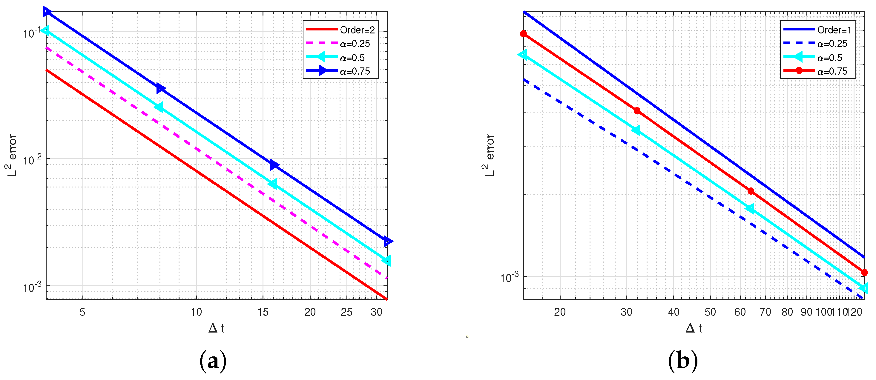
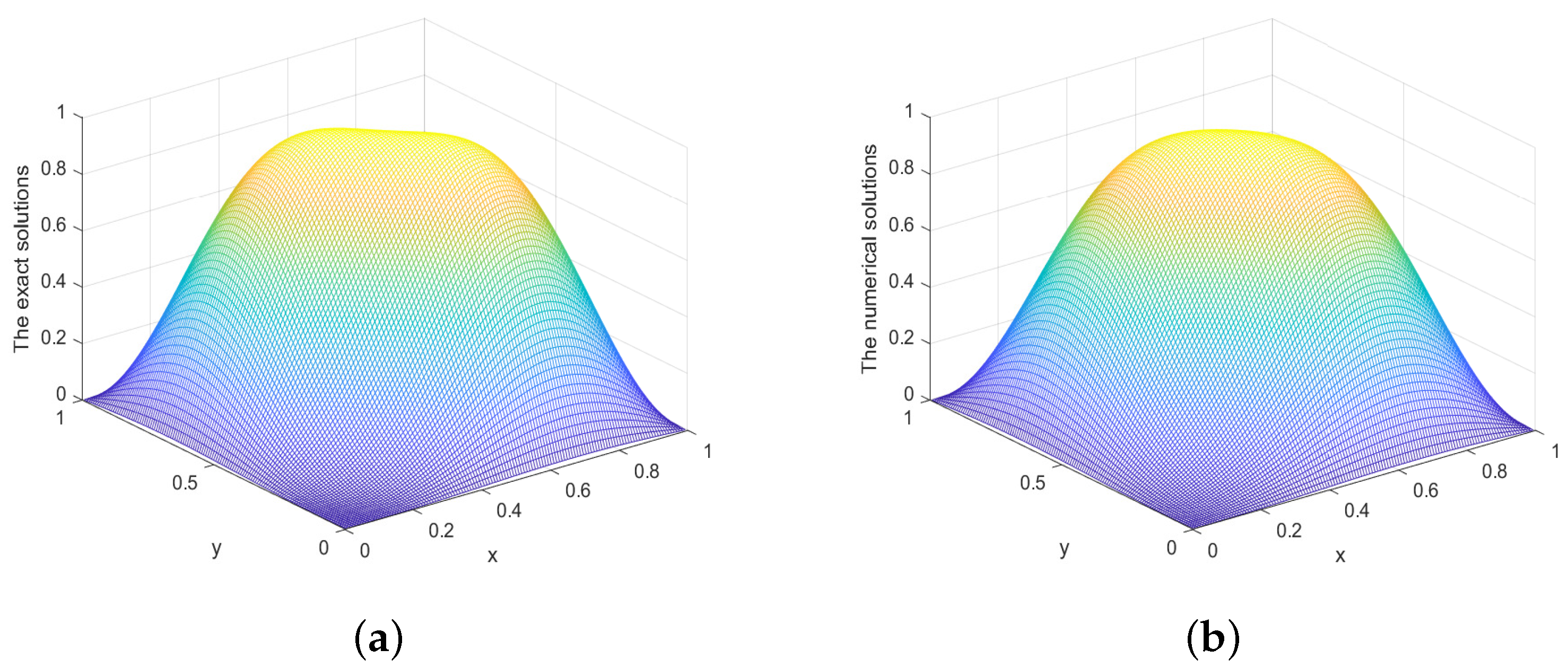
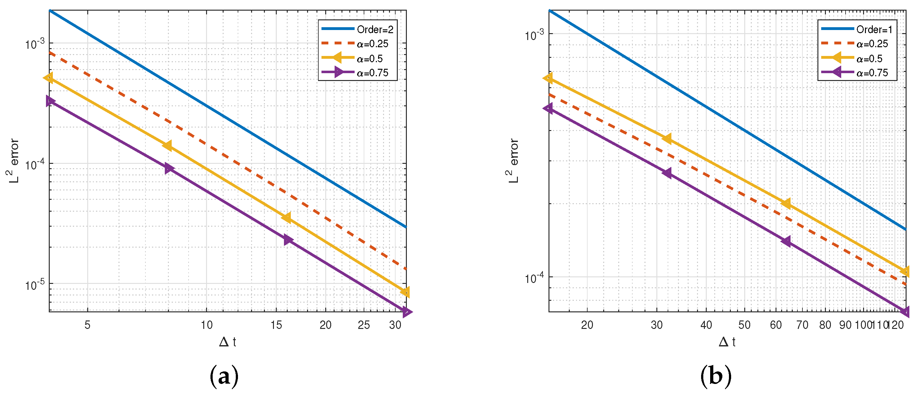
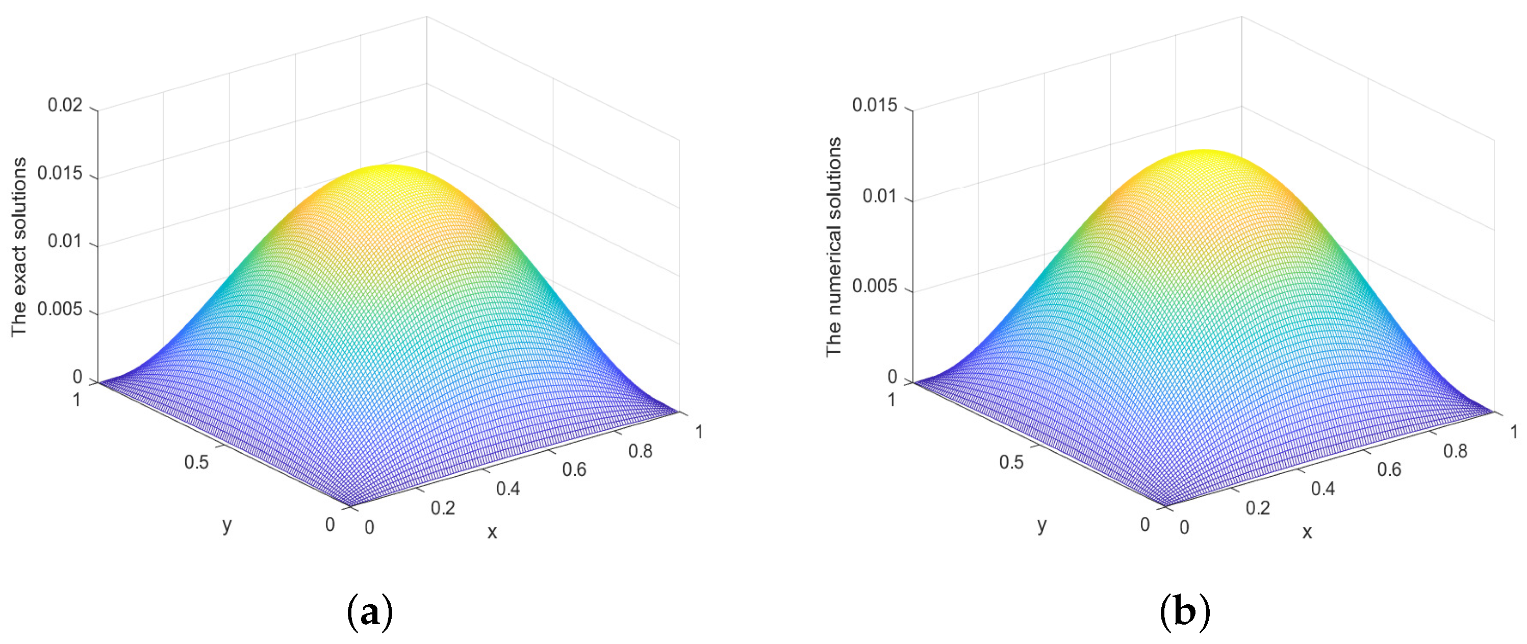
5. Numerical Experiments

In this section, we will describe some numerical experiments to verify our theory.

In the calculation, we set $d=2$, $T=1$, and the domain $\Omega$ as the unit square $[0,1]\times [0,1]$, and we computed the problem (1)–(3) by using the WG finite element schemes (14)–(15). In order to calculate the WG finite element scheme, we selected the parameters $k=1$, $l=0$, and $r=0$. We chose the element $(P_k\left(\mathcal{T}\right),P_l(\partial \mathcal{T}),{\left[P_r\left(\mathcal{T}\right)\right]}^2)$ as $(P_1\left(\mathcal{T}\right),P_0(\partial \mathcal{T}),{\left[P_0\left(\mathcal{T}\right)\right]}^2)$. The basis functions we calculated and selected were $\{1,x,y\}$. And the mesh size was $h=1/M$ for triangular meshes.

We let $u^n$ and $u_h^n$ be the exact solution for (1)–(3) and numerical solution for (14)–(15), respectively. According to the Theorem 2, we gave an error function definition, denoted as

$$Error(h,\tau )=\parallel u_h^n-Q_h{u}^n\parallel ,$$

and

$$rat{e}_x=lo{g}_{{\displaystyle \frac{h_1}{h_2}}}{\displaystyle \frac{Error(h_1,\tau )}{Error(h_2,\tau )}},rat{e}_t=lo{g}_{{\displaystyle \frac{{\tau }_1}{{\tau }_2}}}{\displaystyle \frac{Error(h,{\tau }_1)}{Error(h,{\tau }_2)}}.$$

Example 1. 

In this example, the exact solution was chosen to be

$$u(x,y,t)=sin\left(\pi x\right)sin\left(\pi y\right)-{\displaystyle \frac{t^{\alpha +1}}{\Gamma (\alpha +2)}}sin\left(2\pi x\right)sin\left(2\pi y\right),$$

so that we could obtain the initial condition

$$\psi (x,y)=sin\left(\pi x\right)sin\left(\pi y\right),$$

and the inhomogeneous term

$$f(x,y,t)={\displaystyle \frac{t^{\alpha }}{\Gamma (\alpha +1)}}2{\pi }^{2}sin\left(\pi x\right)sin\left(\pi y\right)-{\displaystyle \frac{t^{\alpha }}{\Gamma (\alpha +1)}}sin\left(2\pi x\right)sin\left(2\pi y\right)-{\displaystyle \frac{8{\pi }^2{t}^{2\alpha +1}}{\Gamma (2\alpha +2)}}sin\left(2\pi x\right)sin\left(2\pi y\right).$$

First, we set $\tau =1/2^{12}$ and we obtained the $L^2$-norm error and the convergence order of the WG finite element fully discrete schemes (14)–(15) for $\alpha =0.25,0.5,0.75,$ respectively. According to the data of

Table 1. The $L^2$ error and space convergence orders when $\tau =1/2^{12}$ at $t=0.5$.

$\mathit{\alpha }$	M	$\parallel {\mathit{u}}_{\mathit{h}}^{\mathit{n}}-{\mathit{Q}}_{\mathit{h}}{\mathit{u}}^{\mathit{n}}\parallel$	${\mathit{rate}}_{\mathit{x}}$
$0.25$	$2^2$ $2^3$ $2^4$ $2^5$	1.500299 $\times {10}^{-1}$ 3.761225 $\times {10}^{-2}$ 9.396687 $\times {10}^{-3}$ 2.340609 $\times {10}^{-3}$	1.99598 2.00098 2.00527
$0.5$	$2^2$ $2^3$ $2^4$ $2^5$	1.453775 $\times {10}^{-1}$ 3.634613 $\times {10}^{-2}$ 9.078598 $\times {10}^{-3}$ 2.265468 $\times {10}^{-3}$	1.99993 2.00126 2.00266
$0.75$	$2^2$ $2^3$ $2^4$ $2^5$	1.435374 $\times {10}^{-1}$ 3.588690 $\times {10}^{-2}$ 8.966046 $\times {10}^{-3}$ 2.239688 $\times {10}^{-3}$	1.99990 2.00091 2.00117

, it is easy to see that the space convergence order was 2. Then, we fixed the space step $h=1/2^7$, we obtained the errors, and the time convergence order was 1 in the $L^2$-norm from

Table 2. The $L^2$ error and time convergence orders when $h=1/2^7$ at $t=0.5$.

$\mathit{\alpha }$	N	$\parallel {\mathit{u}}_{\mathit{h}}^{\mathit{n}}-{\mathit{Q}}_{\mathit{h}}{\mathit{u}}^{\mathit{n}}\parallel$	${\mathit{rate}}_{\mathit{t}}$
$0.25$	$2^4$ $2^5$ $2^6$ $2^7$	8.807003 $\times {10}^{-3}$ 4.846912 $\times {10}^{-3}$ 2.599962 $\times {10}^{-3}$ 1.367762 $\times {10}^{-3}$	0.86159 0.89858 0.92667
$0.5$	$2^4$ $2^5$ $2^6$ $2^7$	1.050071 $\times {10}^{-2}$ 5.538527 $\times {10}^{-3}$ 2.856477 $\times {10}^{-3}$ 1.457183 $\times {10}^{-3}$	0.92291 0.95527 0.97106
$0.75$	$2^4$ $2^5$ $2^6$ $2^7$	9.710630 $\times {10}^{-3}$ 5.066485 $\times {10}^{-3}$ 2.568006 $\times {10}^{-3}$ 1.289339 $\times {10}^{-3}$	0.93858 0.98034 0.99402

. Figure 1 describes the spatial and temporal convergence orders, and it was plotted based on the data ($\alpha$, M, $rat{e}_x$, and $rat{e}_t$) given in Table 1 and Table 2, using the “loglog” function in Matlab. Figure 2 displays the distributions of the numerical solutions and the exact solutions for Example 1, created using the “mesh” function in Matlab 2022a. From Figure 1, we can clearly see that the convergence order of the scheme was 2 in space and 1 in time, and the numerical results conform well to our theoretical analysis. From Figure 2, we can see that the exact solutions and numerical solutions of Example 1 at $t=0.5$ show that the numerical solutions approximate the exact solutions well.

Example 2. 

For the second example, we gave exact solution

$$u(x,y,t)={\displaystyle \frac{t^{\alpha +1}}{\Gamma (\alpha +2)}}x(1-x)y(1-y),$$

with the initial condition

$$\psi (x,y)=0,$$

and the right-hand term

$$f(x,y,t)={\displaystyle \frac{t^{\alpha }}{\Gamma (\alpha +1)}}x(1-x)y(1-y)+{\displaystyle \frac{2t^{2\alpha +1}}{\Gamma (2\alpha +2)}}\left(x(1-x)+y(1-y)\right).$$

First, we fixed the time step $\tau =1/2^{12}$ and obtained the error in the $L^2$-norm. Table 2 shows the error and space convergence with the rate $O\left(h^2\right)$ in $L^2$-norms. Then, we fixed the mesh size $h=1/2^{10}$ and obtained the error in the $L^2$-norm.

Table 3. The $L^2$ error and space convergence orders when $\tau =1/2^{12}$ at $t=0.5$.

$\mathit{\alpha }$	M	$\parallel {\mathit{u}}_{\mathit{h}}^{\mathit{n}}-{\mathit{Q}}_{\mathit{h}}{\mathit{u}}^{\mathit{n}}\parallel$	${\mathit{rate}}_{\mathit{x}}$
$0.25$	$2^2$ $2^3$ $2^4$ $2^5$	8.493773 $\times {10}^{-4}$ 2.244136 $\times {10}^{-4}$ 5.575981 $\times {10}^{-5}$ 1.291414 $\times {10}^{-5}$	1.92025 2.00886 2.11027
$0.5$	$2^2$ $2^3$ $2^4$ $2^5$	5.223547 $\times {10}^{-4}$ 1.400798 $\times {10}^{-4}$ 3.496892 $\times {10}^{-5}$ 8.450654 $\times {10}^{-6}$	1.89878 2.00210 2.04894
$0.75$	$2^2$ $2^3$ $2^4$ $2^5$	3.364420 $\times {10}^{-4}$ 9.127113 $\times {10}^{-5}$ 2.311183 $\times {10}^{-5}$ 5.849509 $\times {10}^{-6}$	1.88213 1.98153 1.98224

shows that the convergence rate with respect to the time step was $O\left(\tau \right)$ which conforms well to our theoretical analysis. Also, from Figure 3, it can be clearly observed that the convergence order of the scheme was $O\left(h^2\right)$ in space and $O\left(\tau \right)$ in time, which is consistent with our theoretical analysis. Figure 3 describes the spatial and temporal convergence orders, and it was plotted based on the data ($\alpha$, M, $rat{e}_x$, and $rat{e}_t$) given in Table 3 and

Table 4. The $L^2$ error and space convergence orders when $h=1/2^7$ at $t=0.5$.

$\mathit{\alpha }$	N	$\parallel {\mathit{u}}_{\mathit{h}}^{\mathit{n}}-{\mathit{Q}}_{\mathit{h}}{\mathit{u}}^{\mathit{n}}\parallel$	${\mathit{rate}}_{\mathit{t}}$
$0.25$	$2^4$ $2^5$ $2^6$ $2^7$	5.631114 $\times {10}^{-4}$ 3.189182 $\times {10}^{-4}$ 1.743488 $\times {10}^{-4}$ 9.295012 $\times {10}^{-5}$	0.82023 0.87121 0.90745
$0.5$	$2^4$ $2^5$ $2^6$ $2^7$	6.561934 $\times {10}^{-4}$ 3.695099 $\times {10}^{-4}$ 1.998514 $\times {10}^{-4}$ 1.049854 $\times {10}^{-4}$	0.82851 0.88669 0.92874
$0.75$	$2^4$ $2^5$ $2^6$ $2^7$	4.929918 $\times {10}^{-4}$ 2.669213 $\times {10}^{-4}$ 1.396821 $\times {10}^{-4}$ 7.162491 $\times {10}^{-5}$	0.88515 0.93427 0.96361

, using the “loglog” function in Matlab. Figure 4 displays the distributions of the numerical solutions and the exact solutions for Example 2, created using the “mesh” function in Matlab. From Figure 4, we can see that the exact solutions and numerical solutions of Example 2 at $t=0.5$ show that the numerical solutions approximate the exact solutions well.

We present two numerical examples with distinct characteristics. The numerical results, obtained under varying initial conditions, are in agreement with our theoretical findings. Furthermore, by comparing the figure representations of the numerical solutions and the exact solutions, it is evident that the numerical solutions closely approximate the exact solutions.

6. Conclusions

In this article, we extend the WG finite element method to multi-dimensional evolution equations with a weakly singular kernel. A WG finite element fully discrete scheme is presented, accompanied by detailed proofs of its stability and convergence in the $L^2$-norm. To validate the theoretical results, two numerical examples with different initial conditions were implemented. The numerical results confirm both the accuracy of the proposed method in solving evolution equations with weakly singular kernels and the correctness of the theoretical proof. The conclusion supports our research.

Future research will concentrate on extending the current method to nonlinear evolution equations with a weakly singular kernel. And the corresponding numerical theoretical analysis and calculation will be carried out in future work.

References

1. Podlubny, I. Fractional Differential Equations; Academic Press: San Diego, CA, USA, 1999. [Google Scholar]
2. Kilbas, A.; Srivastava, H.; Trujillo, J. Theory and Applications of Fractional Differential Equations; Elsevier: Amsterdam, The Netherlands, 2006. [Google Scholar]
3. Chen, H.; Xu, D. A compact difference scheme for an evolution equation with a weakly singular kernel. Numer. Math. Theoret. Meth. Appl. 2012, 5, 559–572. [Google Scholar]
4. Chen, C.; Thomée, V.; Wahlbin, L. Finite element approximation of a parabolic integro-differential equation with a weakly singular kernel. Math. Comput. 1992, 58, 587–602. [Google Scholar] [CrossRef]
5. Mclean, W.; Thomée, V. Numerical solution of an evolution equation with a positive type memory term. J. Austral. Math. Soc. Ser. B 1993, 35, 23–70. [Google Scholar] [CrossRef]
6. Zhang, H.; Liu, Y.; Yang, X. An efficient ADI difference scheme for the nonlocal evolution problem in three-dimensional space. J. Appl. Math. Comput. 2023, 69, 651–674. [Google Scholar] [CrossRef]
7. Zheng, Z.; Wang, Y. A fast temporal second-order compact finite difference method for two-dimensional parabolic integro-differential equations with weakly singular kernel. J. Comput. Sci. 2025, 87, 102558. [Google Scholar] [CrossRef]
8. Fakhari, H.; Mohebbi, A. Galerkin spectral and finite difference methods for the solution of fourth-order time fractional partial integro-differential equation with a weakly singular kernel. J. Appl. Math. Comput. 2024, 70, 5063–5080. [Google Scholar] [CrossRef]
9. Chen, Y.; Chen, Z.; Huang, Y. An hp-version of the discontinuous Galerkin method for fractional integro-differential equations with weakly singular kernels. BIT Numer. Math. 2024, 64, 27. [Google Scholar] [CrossRef]
10. Yang, X.; Zhang, H.; Zhang, Q.; Yuan, G.; Sheng, Z. The finite volume scheme preserving maximum principle for two-dimensional time-fractional Fokker–Planck equations on distorted meshes. Appl. Math. Lett. 2019, 97, 99–106. [Google Scholar] [CrossRef]
11. Qiu, W.; Xu, D.; Guo, J.; Zhou, J. A time two-grid algorithm based on finite difference method for the two-dimensional nonlinear time fractional mobile/immobile transport model. Numer. Algor. 2020, 85, 39–58. [Google Scholar] [CrossRef]
12. Qiu, W.; Xu, D.; Guo, J. The Crank-Nicolson-type Sinc-Galerkin method for the fourth-order partial integro-differential equation with a weakly singular kernel. Appl. Numer. Math. 2021, 159, 239–258. [Google Scholar] [CrossRef]
13. Yan, Y.; Fairweather, G. Orthogonal spline collocation methods for some partial integro-differential equations. SIAM J. Numer. Anal. 1992, 29, 755–768. [Google Scholar] [CrossRef]
14. Zhang, H.; Yang, X.; Xu, D. An efficient spline collocation method for a nonlinear fourth-order reaction subdiffusion equation. J. Sci. Comput. 2020, 85, 7. [Google Scholar] [CrossRef]
15. Zhao, Y.; Gu, X.; Ostermann, A. A preconditioning technique for an all-at-once system from Volterra subdiffusion equations with graded time steps. J. Sci. Comput. 2021, 88, 11. [Google Scholar] [CrossRef]
16. Rostami, Y. Two approximated techniques for solving of system of two-dimensional partial integral differential equations with weakly singular kernels. Comput. Appl. Math. 2021, 40, 217. [Google Scholar] [CrossRef]
17. Wang, J.; Ye, X. A weak Galerkin finite element method for second-order elliptic problems. J. Comput. Appl. Math. 2013, 241, 103–115. [Google Scholar] [CrossRef]
18. Mu, L.; Wang, J.; Wang, Y.; Ye, X. A computational study of the weak Galerkin method for second order elliptic equations. Numer. Algor. 2012, 63, 753–777. [Google Scholar] [CrossRef]
19. Gao, F.; Mu, L. On L2 error estimate for weak Galerkin finte element for parabolic problems. J. Comput. Math. 2014, 32, 195–204. [Google Scholar]
20. Li, W.; Gao, F.; Cui, J. A weak Galerkin finite element method for nonlinear convection-diffusion equation. Appl. Math. Comput. 2024, 461, 128315. [Google Scholar] [CrossRef]
21. Mu, L.; Wang, J.; Ye, X. Weak Galerkin finite element methods on polytopal Meshes. Int. J. Numer. Anal. Model. 2012, 12, 31–53. [Google Scholar]
22. Wang, C.; Ye, X.; Zhang, S. A Modified weak Galerkin finite element method for the Maxwell equations on polyhedral meshes. J. Comput. Appl. Math. 2024, 448, 115918. [Google Scholar] [CrossRef]
23. Wang, C. Auto-stabilized weak Galerkin finite element methods on polytopal meshes without convexity constraints. J. Comput. Appl. Math. 2025, 466, 116572. [Google Scholar] [CrossRef]
24. Wang, J.; Wang, R.; Zhai, Q.; Zhang, R. A systematic study on weak Galerkin finite element methods for second order elliptic problems. J. Sci. Comput. 2018, 74, 1369–1396. [Google Scholar] [CrossRef]
25. Li, D.; Wang, C.; Wang, J.; Ye, X. Generalized weak Galerkin finite element methods for second order elliptic problems. J. Comput. Appl. Math. 2024, 445, 115833. [Google Scholar] [CrossRef]
26. Zhou, J.; Xu, D.; Dai, X. Weak Galerkin finite element method for the parabolic integro-differential equation with weakly singular kernel. Comput. Appl. Math. 2019, 38, 38. [Google Scholar] [CrossRef]
27. Zhou, J.; Xu, D.; Chen, H. A weak Galerkin finite element method for multi-term time-fractional diffusion equations. East Asian J. Appl. Math. 2018, 8, 181–193. [Google Scholar]
28. Zhou, J.; Xu, D.; Qiu, W.; Qiao, L. An accurate, robust, and efficient weak Galerkin finite element scheme with graded meshes for the time-fractional quasi-linear diffusion equation. Comput. Math. Appl. 2022, 124, 188–195. [Google Scholar] [CrossRef]
29. Tang, T. A finite difference scheme for partial integro-differential equations with a weakly singular kernel. Appl. Numer. Math. 1993, 11, 309–319. [Google Scholar] [CrossRef]
30. Wheeler, M.F. A priori L2 error estimates for Galerkin approximations to parabolic partial differential equations. SIAM J. Numer. Anal. 1973, 10, 723–759. [Google Scholar] [CrossRef]
31. Zhang, H.; Zou, Y.; Xu, Y.; Zhai, Q.; Yue, H. Weak Galerkin finite element method for second order parabolic equations. Int. J. Numer. Anal. Model. 2016, 13, 525–544. [Google Scholar]
Figure 1. The convergence orders when k = 1 . (a) The space convergence orders. (b) The time convergence orders.
Fractalfract 09 00368 g001
Figure 2. The exact solutions and numerical solutions at t = 0.5 . (a) The exact solutions. (b) The numerical solutions.
Fractalfract 09 00368 g002
Figure 3. The convergence orders when k = 1 . (a) The space convergence orders. (b) The time convergence orders.
Fractalfract 09 00368 g003
Figure 4. The exact solutions and numerical solutions at t = 0.5 . (a) The exact solutions. (b) The numerical solutions.
Fractalfract 09 00368 g004