Solitons, Cnoidal Waves and Nonlinear Effects in Oceanic Shallow Water Waves

Abstract

Gravity water waves in the shallow-ocean scenario described by generalized Boussinesq–Broer–Kaup–Whitham (gBBKW) equations are discussed. The residual symmetry and Bäcklund transformation associated with the gBBKW equations are systematically constructed. The time and space evolution of wave velocity and height are explored. Additionally, it is demonstrated that the gBBKW equations are solvable through the consistent Riccati expansion method. Leveraging this property, a novel Bäcklund transformation, solitary wave solution, and soliton–cnoidal wave solution are derived. Furthermore, miscellaneous novel solutions of gBBKW equations are obtained using the modified Sardar sub-equation method. The impact of variations in the diffusion power parameter on wave velocity and height is quantitatively analyzed. The exact solutions of gBBKW equations provide precise description of propagation characteristics for a deeper understanding and the prediction of some ocean wave phenomena.

1. Introduction

Nonlinear equations are widely applied in many branches of natural science, including but not limited to fluid mechanics [1,2], cosmology [3,4,5], field theory [6,7], plasma waves [8,9], geophysics [10], nonlinear optics [11,12], and oceanography [13]. These equations and their solutions furnish essential mathematical frameworks for elucidating complex natural phenomena. Classical methods for deriving exact solutions to nonlinear equations include Painlevé analysis [14,15,16], the Hirota bilinear method [17,18], the inverse scattering transformation method [19], the Darboux transformation method [20,21], symmetry analysis [22,23,24], the Riemann–Hilbert method [25,26], the Bäcklund transformation method [27,28], and so on. Among these, the symmetry method is widely regarded as one of the most systematic and effective approaches. Notably, within symmetry analysis, nonlocal symmetries are capable of generating more diversified forms of solutions that are unattainable through Lie point symmetries alone. This diversity is particularly advantageous for modeling and interpreting a wide array of complex physical phenomena.

It is well known that Painlevé analysis is an effective method with which to study the integrability of nonlinear differential equations. Based on truncated Painlevé expansion, Lou proposed a method to construct the nonlocal symmetry, which is also called residual symmetry [29]. Lou further extended the truncated Painlevé expansion to propose a simpler method to obtain the interaction solutions, which is called the consistent Riccati expansion (CRE) method [30,31]. When a system is CRE-solvable, this method enables the analysis of interactions between solitons and other nonlinear waves. Numerous systems have been demonstrated to exhibit CRE solvability, including the Korteweg–de Vries (KdV) equation [32], the modified Korteweg–de Vries (mKdV) equation [33,34], the Kadomtsev–Petviashvili equation [35], the Kaup–Kupershmidt equation [36,37], and the Boussinesq equation [38,39].

As a novel and robust method that has emerged in recent years for solving nonlinear partial differential equations (NPDEs), the Sardar sub-equation method (SSM) was initially introduced by Rezazadeh et al. [40] to address the (3 + 1)-dimensional Wazwaz–Benjamin–Bona–Mahony equation. Subsequently, Akinyemi et al. developed the modified Sardar sub-equation method (MSSM) [41] as an advanced approach for solving NPDEs. As an extension of the original SSM, the MSSM demonstrates enhanced versatility, enabling it to tackle a broader spectrum of equations. This method has been successfully employed to solve various NPDEs, including Schrödinger equations [42,43,44] and the modified Korteweg–de Vries–Zakharov–Kuznetsov equation [45]. In comparison to traditional methods for deriving exact solutions, the MSSM is capable of generating novel exact solutions characterized by diverse functional forms, such as trigonometric, exponential, and rational functions. For certain nonlinear or strongly coupled systems, the application of classical methods to derive exact solutions may prove challenging. However, the MSSM offers a streamlined approach to simplifying complex nonlinear equations. Its superiority over other methods in solving certain NPDEs is evident in terms of computational efficiency and higher accuracy, making it a valuable tool in the analysis of nonlinear systems.

The Boussinesq equation serves as a fundamental model for describing the propagation of nonlinear dispersive waves in shallow water, while the Broer–Kaup equation characterizes the dynamics of dispersive long waves in shallow-water environments. The Whitham equation, on the other hand, provides a mathematical framework for modeling the propagation of weakly nonlinear, long waves in dispersive media, such as water waves. The generalized Boussinesq–Broer–Kaup–Whitham (gBBKW) system can be regarded as a comprehensive extension that integrates the Boussinesq equation, the Broer–Kaup equation, and the Whitham equation. The gBBKW equations can describe certain gravity water waves in a shallow-ocean scenario in terms of the wave height and surface velocity of the water wave, which can be used to simulate complex wave phenomena in fields such as fluid flow, plasma waves, nonlinear optics, and condensed matter physics. Investigating the symmetries and deriving various forms of exact solutions for the gBBKW equations hold significant importance for advancing our understanding of its physical implications and broadening its practical applications.

We consider the gBBKW equations for certain gravity water waves in a shallow-ocean scenario [46]:

$$\begin{array}{cc}\hfill & u_t+u{u}_x+v_x+\beta u_{xx}=0,\hfill \\ \hfill & v_t+{\left(uv\right)}_x+\alpha u_{xxx}-\beta v_{xx}+\gamma u_x=0,\hfill \end{array}$$

(1)

where the real differentiable function $u(x,t)$ represents the velocity of the water–wave surface along the x axis. The real differentiable function $v(x,t)$ represents the wave height of the water–wave surface. $\alpha ,\beta$, and $\gamma$ are constants representing different diffusion powers. The dispersion effect parameter $\alpha$ controls the dispersion characteristics of the wave. In shallow water waves, the dispersion effect is mainly determined by water depth and wavelength. The dissipation effect parameter $\beta$ reflects the viscous dissipation. It is mainly related to fluid viscosity, wavelength, and water depth. The modulation parameter $\gamma$ mainly reflects the modulation effect of external energy input or dissipation mechanisms on shallow water waves. It is mainly related to the wavelength and water depth.

There have been some related studies for special cases of the gBBKW equations [47,48,49,50,51,52,53,54,55,56,57].

(1) When $\alpha =\gamma =1$ and $\beta =0$, the gBBKW Equation (1) reduces to the Broer-Kaup equations. These equations serve as a mathematical model for describing the bidirectional propagation of water waves in a narrow channel of constant finite depth [47]:

(2) When $\beta =\gamma =0$, $\alpha >0$ or $\beta =\gamma =0$, $\alpha =-{\displaystyle \frac{1}{4}}$, gBBKW Equation (1) reduces to the Kaup–Boussinesq (KB) equations. These equations serve as a mathematical model for describing the dynamics of shallow water waves [48,49]. Specifically, when $\beta =\gamma =0$ and $\alpha ={\displaystyle \frac{1}{3}}$, gBBKW Equation (1) reduces to the (1+1)-dimensional dispersive long-wave equations [50,51]. Furthermore, when $\beta =\gamma =0$ and $\alpha =1$, gBBKW Equation (1) reduces to a variant of the Boussinesq equations [52,53].

(3) When $\gamma =0$, gBBKW Equation (1) reduces to the Whitham–Broer–Kaup (WBK) equations, a model describing the propagation of dispersive long waves in shallow ocean water [54,55].

(4) When $\alpha =\gamma =0$ and $\beta \ne 0$, gBBKW Equation (1) reduces to the classical long-wave equations, a model describing the propagation of diffusive shallow water waves [56].

(5) When $\alpha =\beta =\gamma =0$, gBBKW Equation (1) reduces to a classical dispersiveless long-wave equation, a model describing long waves in shallow water [56].

(6) When $\alpha ={\displaystyle \frac{1}{4}},\beta =0$, and $\gamma =1$, simplified gBBKW Equation (1) models gravity waves in oceanic environments [57].

By adjusting parameters $\alpha$, $\beta$, and $\gamma$, the gBBKW equations can be degraded to the above six cases, but the more general parameter choices of the gBBKW equations achieve a unified description of the complex shallow-water-wave dynamics. In comparison to related studies, the primary novelty of this work lies in the following aspects:

(1) We investigate the gBBKW equations, which unifies and extends several important mathematical models including the Boussinesq equation, the Broer–Kaup equation, and the Whitham equation. The gBBKW equations model gravity waves, long-wave dissipative effects, and nonlinear dispersion uniformly, which is suitable for a wider range of ocean shallow-water scenarios. Diverse wave propagation phenomena in shallow ocean environments are discussed, which have a wide range of applications in the fields of fluid dynamics and nonlinear fluctuations.

(2) After trying a variety of analytical approaches, we derive a wide range of novel solutions for the gBBKW equations, such as a soliton–cnoidal wave solution, multi-soliton solutions, and singular periodic solution. The main characteristics and physical implications of these solutions are thoroughly analyzed. We explicitly analyze the synchronization rule of wave velocity and wave height in the spatial and temporal evolution (e.g., the point of maximum change in the wave velocity corresponds to the trough of the wave height). The exact solutions obtained exhibit features consistent with the characteristics of shallow water waves as modeled by the gBBKW equations, providing precise mathematical representations of the system. These exact solutions are useful as a guide toward obtaining numerical solutions or performing simulations, which can be used as benchmark solutions to test the accuracy and stability of numerical algorithms or to account for the observed anomalous fluctuations.

(3) The impact of variations in parameters $\alpha ,\beta ,$ and $\gamma$ on wave behavior is investigated, which reveals some new phenomena that could not be demonstrated in special cases where these parameters are specific constants. The time and space evolution and the characteristics of wave height and velocity across different wave phenomena are systematically analyzed. Through these analyses, the abstract mathematical solutions are associated with the observable physical phenomena, thus bridging the theoretical model with the actual problem. As a significant nonlinear system modeling gravity water waves in shallow ocean environments, the gBBKW system provides a powerful model for advancing the understanding and prediction of oceanic wave dynamics.

The rest of this paper is organized as follows. In Section 2, the residual symmetry and localization of gBBKW Equation (1) are derived using truncated Painlevé expansion, and kink and soliton solutions are obtained. In Section 3, the CRE solvability of gBBKW Equation (1) is proved. And the soliton solution and interaction solution between a soliton and cnoidal wave are obtained. In Section 4, a concise overview of the MSSM is provided, and a variety of solutions for gBBKW Equation (1) with $\beta =0$ are derived, including a singular periodic wave solution, periodic wave solution, dark periodic singular soliton solution, singular solitary wave solution, and singular soliton solution. Additionally, the physical significance of the selected solutions is discussed alongside graphical representations. Finally, some conclusions are presented in Section 5.

2. Residual Symmetry and Localization

2.1. Residual Symmetry and Bäcklund Transformation

The general form of the truncated Painlevé expansion for gBBKW Equation (1) is

$$u={\displaystyle \sum _{i=0}^{n_1}}{u}_i{f}^{i-n_1},v={\displaystyle \sum _{j=0}^{n_2}}{v}_j{f}^{j-n_2},$$

(2)

where $u_i(0\le i\le n_1)$, $v_j(0\le j\le n_2)$, and singular manifold f$(f\ne 0)$ are undetermined functions of variables x and t. According to the homogeneous balance principle, we choose $n_1=1$ and $n_2=2$ in (2), which can balance the highest derivative and nonlinear terms in (1). Hence,

$$u={\displaystyle \frac{u_0}{f}}+u_1,v={\displaystyle \frac{v_0}{f^2}}+{\displaystyle \frac{v_1}{f}}+v_2.$$

(3)

Substituting Equation (3) into gBBKW Equation (1), collecting coefficients corresponding to different powers of f, and equating them to zero, we obtain

$$\begin{array}{cc}\hfill & u_0=2\sqrt{\alpha +{\beta }^2}{f}_x,v_0=2(\beta \sqrt{\alpha +{\beta }^2}-\alpha -{\beta }^2)f_x^2,\hfill \\ \hfill & u_1=-{\displaystyle \frac{f_t+\sqrt{\alpha +{\beta }^2}{f}_{xx}}{f_x}},v_1=2(\alpha +{\beta }^2-\beta \sqrt{\alpha +{\beta }^2})f_{xx},\hfill \\ \hfill & v_2=(\sqrt{\alpha +{\beta }^2}-\beta )({\displaystyle \frac{f_{xx}{f}_t+\sqrt{\alpha +{\beta }^2}{f}_{xx}^2}{f_x^2}}-{\displaystyle \frac{f_{xt}+\sqrt{\alpha +{\beta }^2}{f}_{xxx}}{f_x}})-\gamma ,\hfill \end{array}$$

(4)

where f satisfies the following Schwarzian equation:

$$C_t+2\sqrt{\alpha +{\beta }^2}{C}_{xx}+(\alpha +{\beta }^2)S_x-C{C}_x=0,$$

(5)

with $C={\displaystyle \frac{f_t}{f_x}},S={\displaystyle \frac{f_{xxx}}{f_x}}-{\displaystyle \frac{3f_{xx}^2}{2f_x^2}}.$

Lemma 1.

The Schwarzian equation remains invariant under Möbius transformation.

Proof. 

Consider

$$C\left(f\right)={\displaystyle \frac{f_t}{f_x}},S\left(f\right)={\displaystyle \frac{f_{xxx}}{f_x}}-{\displaystyle \frac{3f_{xx}^2}{2f_x^2}}.$$

(6)

The Möbius transformations [58] is

$$\phi :f\to {\displaystyle \frac{af+b}{cf+d}}(ad\ne bc),$$

which means

$$\phi \left(f\right)={\displaystyle \frac{af+b}{cf+d}}.$$

(7)

Then,

$$\begin{array}{cc}\hfill & \phi {\left(f\right)}_t={\displaystyle \frac{K{f}_t}{{(cf+d)}^2}},\phi {\left(f\right)}_x={\displaystyle \frac{K{f}_x}{{(cf+d)}^2}},\hfill \\ \hfill & \phi {\left(f\right)}_{xx}={\displaystyle \frac{K{f}_{xx}}{{(cf+d)}^2}}-{\displaystyle \frac{2cK{f}_x^2}{{(cf+d)}^3}},\hfill \\ \hfill & \phi {\left(f\right)}_{xxx}={\displaystyle \frac{K{f}_{xxx}}{{(cf+d)}^2}}-{\displaystyle \frac{6cK{f}_x{f}_{xx}}{{(cf+d)}^3}}+{\displaystyle \frac{6c^{2}K{f}_x^3}{{(cf+d)}^4}},\hfill \end{array}$$

(8)

where $K=ad-bc$. By combining Equations (6) and (8), we can derive

$$\begin{array}{cc}\hfill & C\left(\phi \left(f\right)\right)=C(\phi \circ f)={\displaystyle \frac{\phi {\left(f\right)}_t}{\phi {\left(f\right)}_x}}={\displaystyle \frac{\frac{K{f}_t}{{(cf+d)}^2}}{\frac{K{f}_x}{{(cf+d)}^2}}}={\displaystyle \frac{f_t}{f_x}}=C\left(f\right),\hfill \\ \hfill & \begin{array}{cc}\hfill S\left(\phi \right(f\left)\right)& =S(\phi \circ f)={\displaystyle \frac{\phi {\left(f\right)}_{xxx}}{\phi {\left(f\right)}_x}}-{\displaystyle \frac{3\phi {\left(f\right)}_{xx}^2}{2\phi {\left(f\right)}_x^2}}\hfill \\ \hfill & ={\displaystyle \frac{f_{xxx}}{f_x}}-{\displaystyle \frac{6c{f}_{xx}}{cf+d}}+{\displaystyle \frac{6c^2{f}_x^2}{{(cf+d)}^2}}-{\displaystyle \frac{3}{2}}{({\displaystyle \frac{f_{xx}}{f_x}}-{\displaystyle \frac{2c{f}_x}{cf+d}})}^2\hfill \\ \hfill & =S\left(f\right).\hfill \end{array}\hfill \end{array}$$

(9)

Therefore, $C(\phi \circ f)=C\left(f\right)$ and $S(\phi \circ f)=S\left(f\right)$, which means Schwarzian Equation (5) remains invariant under Möbius transformation. □

In combining Lemma 1, Schwarzian Equation (5) possesses three symmetries:

$${\sigma }^f=c_0,{\sigma }^f=c_{1}f,{\sigma }^f=c_2{f}^2.$$

Based on the preceding analysis, the following Bäcklund transformation theorem can be deduced.

Theorem 1.

If f satisfies Schwarzian Equation (5), then

$$\begin{array}{cc}\hfill & u={\displaystyle \frac{2\sqrt{\alpha +{\beta }^2}{f}_x}{f}}-{\displaystyle \frac{f_t+\sqrt{\alpha +{\beta }^2}{f}_{xx}}{f_x}},\hfill \\ \hfill & \begin{array}{cc}\hfill v=& {\displaystyle \frac{2(\beta \sqrt{\alpha +{\beta }^2}-\alpha -{\beta }^2)f_x^2}{f^2}}+{\displaystyle \frac{2(\alpha +{\beta }^2-\beta \sqrt{\alpha +{\beta }^2})f_{xx}}{f}}\hfill \\ \hfill & +(\sqrt{\alpha +{\beta }^2}-\beta )({\displaystyle \frac{f_{xx}{f}_t+\sqrt{\alpha +{\beta }^2}{f}_{xx}^2}{f_x^2}}-{\displaystyle \frac{f_{xt}+\sqrt{\alpha +{\beta }^2}{f}_{xxx}}{f_x}})-\gamma \hfill \end{array}\hfill \end{array}$$

(10)

is a solution of gBBKW Equation (1).

According to residual symmetry theorem [29], the residual symmetry of gBBKW Equation (1) can be derived as follows:

$$\begin{array}{cc}\hfill & {\sigma }^u=2\sqrt{\alpha +{\beta }^2}{f}_x,\hfill \\ \hfill & {\sigma }^v=2(\alpha +{\beta }^2-\beta \sqrt{\alpha +{\beta }^2})f_{xx}.\hfill \end{array}$$

(11)

To determine the group of residual symmetry,

$$\begin{array}{cc}& u\to \overline{u}\left(\epsilon \right)=u+\epsilon {\sigma }^u,\hfill \\ & v\to \overline{v}\left(\epsilon \right)=v+\epsilon {\sigma }^v,\hfill \end{array}$$

we are supposed to solve the following initial value problem:

$$\begin{array}{cc}\hfill & {\displaystyle \frac{d\overline{u}\left(\epsilon \right)}{d\epsilon }}=2\sqrt{\alpha +{\beta }^2}\overline{f}{\left(\epsilon \right)}_x,\overline{u}\left(\epsilon \right){|}_{\epsilon =0}=u,\hfill \\ \hfill & {\displaystyle \frac{d\overline{v}\left(\epsilon \right)}{d\epsilon }}=2(\alpha +{\beta }^2-\beta \sqrt{\alpha +{\beta }^2})\overline{f}{\left(\epsilon \right)}_{xx},\overline{v}\left(\epsilon \right){|}_{\epsilon =0}=v,\hfill \end{array}$$

(12)

where $\epsilon$ is an infinitesimal parameter.

However, directly solving initial value problem (12) is non-trivial. Consequently, the nonlocal symmetry should be localized to a Lie point symmetry within an extended system. To achieve this, auxiliary variables are introduced:

$$g=f_x,h=f_{xx}.$$

(13)

Thus, a closed prolonged system incorporating Equations (1), (5) and (13) can be constructed, and the corresponding linearized equations for the system are derived as follows:

$$\begin{array}{ccc}& & \begin{array}{cc}& {\sigma }_t^u+{\sigma }^u{u}_x+u{\sigma }_x^u+{\sigma }_x^v+\beta {\sigma }_{xx}^u=0,\hfill \\ & {\sigma }_t^v+{\sigma }_x^{u}v+u_x{\sigma }^v+{\sigma }^u{v}_x+u{\sigma }_x^v+\alpha {\sigma }_{xxx}^u-\beta {\sigma }_{xx}^v+\gamma {\sigma }_x^u=0,\hfill \end{array}\hfill \end{array}$$

(14)

$$\begin{array}{ccc}& & \begin{array}{cc}& [{\sigma }_{tt}^f+2\sqrt{\alpha +{\beta }^2}{\sigma }_{xxt}^f+(\alpha +{\beta }^2){\sigma }_{4x}^f]f_x^{-1}+[-{\sigma }_x^f{f}_{tt}\hfill \\ & -2\sqrt{\alpha +{\beta }^2}{\sigma }_x^f{f}_{xxt}-(\alpha +{\beta }^2){\sigma }_x^f{f}_{4x}-2{\sigma }_{xt}^f{f}_t-4\sqrt{\alpha +{\beta }^2}{\sigma }_{xt}^f{f}_{xx}\hfill \\ & -2{\sigma }_t^f{f}_{xt}-2\sqrt{\alpha +{\beta }^2}{\sigma }_t^f{f}_{xxx}-4\sqrt{\alpha +{\beta }^2}{\sigma }_{xx}^f{f}_{xt}-4(\alpha +{\beta }^2){\sigma }_{xx}^f{f}_{xxx}\hfill \\ & -2\sqrt{\alpha +{\beta }^2}{\sigma }_{xxx}^f{f}_t-4(\alpha +{\beta }^2){\sigma }_{xxx}^f{f}_{xx}]f_x^{-2}+[4{\sigma }_x^f{f}_{xt}{f}_t\hfill \\ & +8\sqrt{\alpha +{\beta }^2}{\sigma }_x^f{f}_{xx}{f}_{xt}+4\sqrt{\alpha +{\beta }^2}{\sigma }_x^f{f}_{xxx}{f}_t\hfill \\ & +8(\alpha +{\beta }^2){\sigma }_x^f{f}_{xx}{f}_{xxx}+{\sigma }_{xx}^f{f}_t^2+8\sqrt{\alpha +{\beta }^2}{\sigma }_{xx}^f{f}_{xx}{f}_t\hfill \\ & +9(\alpha +{\beta }^2){\sigma }_{xx}^f{f}_{xx}^2+2{\sigma }_t^f{f}_{xx}{f}_t+4\sqrt{\alpha +{\beta }^2}{\sigma }_t^f{f}_{xx}^2]f_x^{-3}\hfill \\ & +[-3{\sigma }_x^f{f}_{xx}{f}_t^2-12\sqrt{\alpha +{\beta }^2}{\sigma }_x^f{f}_{xx}^2{f}_t-9(\alpha +{\beta }^2){\sigma }_x^f{f}_{xx}^3]f_x^{-4}=0,\hfill \end{array}\hfill \end{array}$$

(15)

$$\begin{array}{ccc}& & {\sigma }^g-{\sigma }_x^f=0,{\sigma }^h-{\sigma }_{xx}^f=0.\hfill \end{array}$$

(16)

Using Equations (11), (13) and (14), we have ${\sigma }^u=2\sqrt{\alpha +{\beta }^2}g$ and ${\sigma }^v=2(\alpha +{\beta }^2-\beta \sqrt{\alpha +{\beta }^2})h$. According to the Möbius transformation analysis, the point symmetry form of variable f can be expressed as ${\sigma }^f=c_0+c_{1}f+c_2{f}^2$. It can be derived that ${\sigma }^f=-f^2$ is a solution of Equation (15). Using Equation (16), we can obtain ${\sigma }^g=-2fg$ and ${\sigma }^h=-2g^2-2fh$. Therefore, the Lie point symmetry of the prolonged system can be derived by solving Equations (14)–(16), yielding

$$\begin{array}{cc}\hfill & {\sigma }^u=2\sqrt{\alpha +{\beta }^2}g,{\sigma }^v=2(\alpha +{\beta }^2-\beta \sqrt{\alpha +{\beta }^2})h,\hfill \\ & {\sigma }^f=-f^2,{\sigma }^g=-2fg,{\sigma }^h=-2g^2-2fh.\hfill \end{array}$$

(17)

The corresponding Lie point symmetry vector field is given by

$$\begin{array}{c}\hfill \underline{V}=2\sqrt{\alpha +{\beta }^2}g{\displaystyle \frac{\partial }{\partial u}}+2(\alpha +{\beta }^2-\beta \sqrt{\alpha +{\beta }^2})h{\displaystyle \frac{\partial }{\partial v}}-f^2{\displaystyle \frac{\partial }{\partial f}}-2fg{\displaystyle \frac{\partial }{\partial g}}-(2g^2+2fh){\displaystyle \frac{\partial }{\partial h}}.\end{array}$$

Next, we give the finite symmetry transformation theorem, which is derived by applying the finite transformation associated with Lie point symmetry (17).

Theorem 2.

If $\{u,v,f,g,h\}$ is a solution of prolonged system (1), (5), and (13), then

$$\begin{array}{cc}\hfill & \overline{u}\left(\epsilon \right)=u+{\displaystyle \frac{2\epsilon g\sqrt{\alpha +{\beta }^2}}{1+\epsilon f}},\overline{v}\left(\epsilon \right)=v+2\epsilon (\alpha +{\beta }^2-\beta \sqrt{\alpha +{\beta }^2}){\displaystyle \frac{h+\epsilon fh-\epsilon g^2}{{(1+\epsilon f)}^2}},\hfill \\ \hfill & \overline{f}\left(\epsilon \right)={\displaystyle \frac{f}{1+\epsilon f}},\overline{g}\left(\epsilon \right)={\displaystyle \frac{g}{{(1+\epsilon f)}^2}},\overline{h}\left(\epsilon \right)={\displaystyle \frac{h}{{(1+\epsilon f)}^2}}-{\displaystyle \frac{2\epsilon g^2}{{(1+\epsilon f)}^3}}\hfill \end{array}$$

(18)

is also a solution of this prolonged system.

Proof. 

According to Lie’s first fundamental theorem [59], the initial value problem corresponding to Lie point symmetry (17) can be expressed as

$$\begin{array}{cc}\hfill & {\displaystyle \frac{d\overline{u}\left(\epsilon \right)}{d\epsilon }}=2\sqrt{\alpha +{\beta }^2}\overline{g}\left(\epsilon \right),\overline{u}\left(\epsilon \right){|}_{\epsilon =0}=u,\hfill \\ \hfill & {\displaystyle \frac{d\overline{v}\left(\epsilon \right)}{d\epsilon }}=2(\alpha +{\beta }^2-\beta \sqrt{\alpha +{\beta }^2})\overline{h}\left(\epsilon \right),\overline{v}\left(\epsilon \right){|}_{\epsilon =0}=v,\hfill \\ \hfill & {\displaystyle \frac{d\overline{f}\left(\epsilon \right)}{d\epsilon }}=-{\overline{f}}^2\left(\epsilon \right),\overline{f}\left(\epsilon \right){|}_{\epsilon =0}=f,\hfill \\ \hfill & {\displaystyle \frac{d\overline{g}\left(\epsilon \right)}{d\epsilon }}=-2\overline{f}\left(\epsilon \right)\overline{g}\left(\epsilon \right),\overline{g}\left(\epsilon \right){|}_{\epsilon =0}=g,\hfill \\ \hfill & {\displaystyle \frac{d\overline{h}\left(\epsilon \right)}{d\epsilon }}=-2{\overline{g}}^2\left(\epsilon \right)-2\overline{f}\left(\epsilon \right)\overline{h}\left(\epsilon \right),\overline{h}\left(\epsilon \right){|}_{\epsilon =0}=h.\hfill \end{array}$$

(19)

Through the resolution of initial value problem (19), solution (18) is obtained, which completes the proof of Theorem 2. □

2.2. Soliton Solutions

Case 1. One-soliton solution.

Based on Theorem 2, new solutions can be derived from various seed solutions of gBBKW Equation (1) and its associated Schwarzian Equation (5). Take the trivial seed solution of gBBKW Equation (1) as

$$u=0,v=0,$$

(20)

and assume the one-soliton solution takes the following form:

$$f=A+B_1{e}^{p_{1}x+q_{1}t},$$

(21)

where $A,B_1,p_1$, and $q_1$ are arbitrary constants. Substituting Equations (20) and (21) into $u_1$ and $v_2$ in Equation (4) and Schwarzian Equation (5), we obtain

$$q_1=-\sqrt{\alpha +{\beta }^2}{p}_1^2,\gamma =0.$$

(22)

Substituting Equations (20)–(22) into Equation (18), the one-soliton solution of gBBKW Equation (1) is obtained as follows:

$$\begin{array}{cc}\hfill & u={\displaystyle \frac{2\epsilon \sqrt{\alpha +{\beta }^2}{p}_1{B}_1{e}^{p_{1}x-\sqrt{\alpha +{\beta }^2}{p}_1^{2}t}}{1+\epsilon (A+B_1{e}^{p_{1}x-\sqrt{\alpha +{\beta }^2}{p}_1^{2}t})}},\hfill \\ \hfill & v={\displaystyle \frac{2\epsilon (\alpha +{\beta }^2-\beta \sqrt{\alpha +{\beta }^2})p_1^2{B}_1{e}^{p_{1}x-\sqrt{\alpha +{\beta }^2}{p}_1^{2}t}(1+A\epsilon )}{{[1+\epsilon (A+B_1{e}^{p_{1}x-\sqrt{\alpha +{\beta }^2}{p}_1^{2}t})]}^2}}.\hfill \end{array}$$

(23)

We further examine the space–time evolution of wave velocity and wave height, along with the impact of variations in the diffusion power parameter on wave velocity and wave height.

(1) The evolution of wave velocity and wave height.

The parameters in Equation (23) are chosen as $\alpha =-{\displaystyle \frac{1}{2}}, \beta =1, \epsilon =1, p_1=-1, A=2$, and $B_1=3$. This yields the kink solution for u and the dark one-soliton solution for v, as illustrated in Figure 1 and Figure 2.

Figure 1a illustrates a kink-type wave for u, which undergoes a smooth transition from one stable state to another within the spatial domain. In contrast, Figure 2a depicts a dark one-soliton wave for v. From Figure 1b and Figure 2b, it is observed that the wave propagates leftward over time while maintaining its waveform without distortion.

A comparison of Figure 1b and Figure 2b reveals that nonlinear effects and shallow-water effects significantly influence wave velocity and height:

(i) For the same time, the positions where wave velocity and height undergo changes exhibit consistency. Specifically, the position where wave velocity changes corresponds to the position where wave height changes, while the position where wave velocity stabilizes aligns with the position where wave height stabilizes.

(ii) The point with the highest tangent slope in Figure 1b corresponds to the same x-coordinate as the lowest point in Figure 2b. This suggests that the position where the wave velocity undergoes the most significant change aligns with the wave trough. In fact, regions where wave velocity changes most prominently often coincide with the peaks or troughs of shallow water waves. This phenomenon arises because peaks and troughs represent points of maximum energy density during wave propagation. At these locations, the amplitude reaches its peak, resulting in energy concentration and, consequently, more pronounced changes in wave velocity. These variations may be attributed to changes in water depth, submarine topography, or other oceanic physical factors.

(2) The influence of changes in the diffusion power parameter on wave velocity and wave height.

For $t=1$, different values of the diffusion power parameter $\alpha$ are substituted into Equation (23), while keeping the remaining parameters consistent with those used in Figure 1 and Figure 2. The resulting variations in wave velocity and wave height for different $\alpha$ are illustrated in Figure 3.

For $t=1$, different values of $\beta$ are substituted into Equation (23), while the remaining parameters are held consistent with those used in Figure 1 and Figure 2. The resulting variations in wave velocity and height for different $\beta$ are illustrated in Figure 4.

From Figure 3 and Figure 4, it is evident that variations in the diffusion power parameters significantly influence wave behavior, as summarized below:

(i) For wave velocity, as $\alpha$ or the absolute value of $\beta$ increases, the curve corresponding to wave velocity becomes steeper, indicating heightened sensitivity to spatial variations. Additionally, the amplitude of the change in wave velocity at the kink increases with the increase in $\alpha$ or the absolute value of $\beta$. Notably, when $\beta$ takes opposite numbers, the wave velocity remains unchanged.

(ii) For wave height, when $\alpha$ is negative, the trough of the dark soliton deepens as $\alpha$ decreases. Conversely, when $\alpha$ is positive, the peak of the bright soliton rises with increasing $\alpha$. Similarly, for negative values of $\beta$, the peak of the bright soliton increases as $\beta$ decreases, while for positive values of $\beta$, the trough of the dark soliton becomes lower as $\beta$ increases.

The temporal variations in wave velocity and wave height exhibit characteristics analogous to their spatial variations.

Case 2. Multi-soliton solutions.

Take the trivial seed solution of the gBBKW Equation (1) as

$$u=0,v=0,$$

(24)

and assume the multi-soliton solution takes the following form:

$$f=A+{\displaystyle \sum _{i=1}^N}{B}_i{e}^{p_{i}x+q_{i}t},$$

(25)

where $A,B_i,p_i$, and $q_i$ ($i=1,2,...N$) are arbitrary constants. Substituting Equations (24) and (25) into $u_1$ and $v_2$ in Equation (4) and Schwarzian Equation (5), we obtain

$$q_i=-\sqrt{\alpha +{\beta }^2}{p}_i^2,\gamma =0.$$

(26)

In substituting Equations (24)–(26) into Equation (18), the multi-soliton solution of the gBBKW Equation (1) is obtained as

$$\begin{array}{ccc}\hfill u& =& {\displaystyle \frac{2\epsilon \sqrt{\alpha +{\beta }^2}{\displaystyle \sum _{i=1}^N}{p}_i{B}_i{e}^{p_{i}x-\sqrt{\alpha +{\beta }^2}{p}_i^{2}t}}{1+\epsilon (A+{\displaystyle \sum _{i=1}^N}{B}_i{e}^{p_{i}x-\sqrt{\alpha +{\beta }^2}{p}_i^{2}t})}},\hfill \\ \hfill v& =& 2\epsilon (\alpha +{\beta }^2-\beta \sqrt{\alpha +{\beta }^2})({\displaystyle \frac{{\displaystyle \sum _{i=1}^N}{p}_i^2{B}_i{e}^{p_{i}x-\sqrt{\alpha +{\beta }^2}{p}_i^{2}t}}{1+\epsilon (A+{\displaystyle \sum _{i=1}^N}{B}_i{e}^{p_{i}x-\sqrt{\alpha +{\beta }^2}{p}_i^{2}t})}}\hfill \end{array}$$

(27)

$$\begin{array}{ccc}& & -{\displaystyle \frac{\epsilon {\left({\displaystyle \sum _{i=1}^N}{p}_i{B}_i{e}^{p_{i}x-\sqrt{\alpha +{\beta }^2}{p}_i^{2}t}\right)}^2}{{(1+\epsilon (A+{\displaystyle \sum _{i=1}^N}{B}_i{e}^{p_{i}x-\sqrt{\alpha +{\beta }^2}{p}_i^{2}t}))}^2}}).\hfill \end{array}$$

(28)

By adjusting the value of N in (27) and (28), we can study the interactions and dynamic behavior between solitons of different numbers. When $N>1$, it indicates multi-soliton solutions, which can reveal complex physical processes such as interactions and energy exchange between solitons.

(1) Two-soliton solution. The two-kink solution u and two-soliton solution v are obtained (c.f. Figure 5 and Figure 6) with $N=2, \alpha =-{\displaystyle \frac{1}{2}}, \beta =1, \epsilon =1, p_1=-1, p_2=1, A=2,$ and $B_1=3, B_2=1$ in Equations (27) and (28).

It can be found that the wave exhibits the following characteristics:

(i) Figure 5a,b illustrate that u in the solution manifests as a two-kink-type wave, while Figure 6a,b depict a two-soliton wave for v. From Figure 5c, it is evident that wave velocity increases over space in some areas. Additionally, Figure 6c reveals that the distance between the two troughs expands over time.

(ii) In comparing Figure 5c and Figure 6c, it can be found that for the same time, the position where wave velocity changes aligns with the position where wave height changes, while the position where the wave velocity tends to stabilize corresponds to the position where the wave height tends to stabilize. Overall, there is consistency in the location where the wave velocity and wave height change. Furthermore, the positions where the wave velocity changes the most correspond to the lowest points of the wave height, respectively.

(2) Three-soliton solution. The parameters in Equations (27) and (28) are chosen as $N=3, \alpha =-{\displaystyle \frac{1}{2}}, \beta =1, \epsilon =1, p_1=-1, p_2=1, p_3={\displaystyle \frac{5}{2}}, A=2, B_1=3, B_2=1$, and $B_3=2$. This yields the three-kink solution for u and the three-soliton solution for v, as illustrated in Figure 7 and Figure 8.

From Figure 7a,b, it is evident that u in the solution manifests as a three-kink-type wave, while Figure 8a,b illustrate that v in the solution takes the form of a three-soliton wave. Figure 7c clearly demonstrates that the velocity of the water wave increases over space in some areas. Additionally, Figure 8c reveals that the distance between the three troughs expands over time. Notably, the positions where wave velocity and wave height change remain consistent.

Remark 1.

(1) The kink solution u can describe discontinuous changes in wave velocity, which may arise from variations in ocean topography or other physical processes. The kink solutions corresponding to the wave velocity are conducive to understanding how the energy of waves is transferred in different areas, particularly in the regions where the wave velocity varies.

(2) The multi-soliton solutions corresponding to wave height v can describe the wave height of multiple solitary waves interacting in shallow water.

3. CRE Solvability and Interaction Solutions

3.1. CRE Solvability

The CRE method [30,31] is an effective approach for constructing new interaction solutions to nonlinear differential systems. The following is a brief introduction to this method. Consider a given NPDE

$$P(u,u_t,u_x,u_{xx},u_{xt},\dots )=0,$$

(29)

where P is a function of u and its derivatives. The objective is to obtain solutions in the form of the following truncated expansion:

$$u={\displaystyle \sum _{i=0}^n}{u}_i{R}^{n-i}\left(w\right),w=w(x,t).$$

(30)

Here, $R\left(w\right)$ satisfies the following Riccati equation:

$$R^{\prime }\left(w\right)=a_0+a_{1}R\left(w\right)+a_2{R}^2\left(w\right),$$

(31)

where $a_0,a_1$, and $a_2$ are arbitrary constants. The value of n can be determined using the homogeneous balance principle, which involves balancing the highest-order derivative term and nonlinear term in Equation (29). Substituting Equations (30) and (31) into Equation (29) yields an equation for $R\left(w\right)$. Setting the coefficients of different powers of $R\left(w\right)$ to zero, we can obtain the expression for $u_i$ and the compatibility equation for w in many integrable systems.

Based on the CRE method, the solution of gBBKW Equation (1) can be expressed as

$$\begin{array}{c}\hfill u=u_{0}R\left(w\right)+u_1,v=v_0{R}^2\left(w\right)+v_{1}R\left(w\right)+v_2.\end{array}$$

(32)

Substituting Equations (31) and (32) into gBBKW Equation (1) and setting the coefficients of different powers of $R\left(w\right)$ to zero yields an overdetermined system of partial differential equations for $u_0,u_1,v_0,v_1$, and $v_2$. Solving this system, we can obtain

$$\begin{array}{ccc}\hfill & & \begin{array}{cc}\hfill & v_0=-2a_2^2(\alpha +{\beta }^2+\beta \sqrt{\alpha +{\beta }^2})w_x^2,u_1={\displaystyle \frac{-w_t+\sqrt{\alpha +{\beta }^2}(w_{xx}+a_1{w}_x^2)}{w_x}},\hfill \\ \hfill & u_0=2a_2\sqrt{\alpha +{\beta }^2}{w}_x,v_1=-2a_2(\alpha +{\beta }^2+\beta \sqrt{\alpha +{\beta }^2})(w_{xx}+a_1{w}_x^2),\hfill \end{array}\hfill \end{array}$$

(33)

$$\begin{array}{ccc}\hfill & & \begin{array}{cc}\hfill v_2=& -{\displaystyle \frac{-w_x{w}_{xt}+w_{xx}{w}_t+\sqrt{\alpha +{\beta }^2}(w_x{w}_{xxx}+a_1{w}_x^2{w}_{xx}-w_{xx}^2+2a_0{a}_2{w}_x^4)}{w_x^2}}\hfill \\ \hfill & \times (\sqrt{\alpha +{\beta }^2}+\beta )-\gamma \hfill \end{array}\hfill \end{array}$$

(34)

with w satisfying the following Schwarzian equation:

$${\overline{C}}_t-2\sqrt{\alpha +{\beta }^2}{\overline{C}}_{xx}+(\alpha +{\beta }^2){\overline{S}}_x-\overline{C}{\overline{C}}_x-(\alpha +{\beta }^2)\delta w_x{w}_{xx}=0,$$

(35)

where $\overline{C}={\displaystyle \frac{w_t}{w_x}},\overline{S}={\displaystyle \frac{w_{xxx}}{w_x}}-{\displaystyle \frac{3w_{xx}^2}{2w_x^2}},$ and $\delta =a_1^2-4a_0{a}_2$.

Through the preceding analysis, gBBKW Equation (1) has a truncated Painlevé expansion solution based on Riccati Equation (31). Consequently, it can be concluded that gBBKW Equation (1) is CRE-solvable [30].

Remark 2.

In the framework of CRE solvability, we use Riccati Equation (31) as the key tool to construct the solution of gBBKW equations. By substituting (31) and (32) into the gBBKW equations, we can transform them into an overdetermined system of partial differential equations, and $w(x,t)$ is required to satisfy Schwarzian Equation (35). As the discriminant of the Riccati equation, $\delta =a_1^2-4a_0{a}_2$ determines the type of solutions. In (35), the introduction of δ bounds the topological property of the Riccati solution to the integrability condition of the Schwarzian equation.

Furthermore, a new Bäcklund transformation between the solution u and v of gBBKW Equation (1) with $R\left(w\right)$ of Riccati Equation (31) can be constructed as follows.

Theorem 3.

If w satisfies Equation (35), then

$$\begin{array}{cc}\hfill & u={\displaystyle \frac{-w_t+\sqrt{\alpha +{\beta }^2}{w}_{xx}+a_1\sqrt{\alpha +{\beta }^2}{w}_x^2}{w_x}}+2a_2\sqrt{\alpha +{\beta }^2}{w}_{x}R\left(w\right),\hfill \\ \hfill & \begin{array}{cc}\hfill v=& -{\displaystyle \frac{-w_x{w}_{xt}+w_{xx}{w}_t+\sqrt{\alpha +{\beta }^2}(w_x{w}_{xxx}+a_1{w}_x^2{w}_{xx}-w_{xx}^2+2a_0{a}_2{w}_x^4)}{w_x^2}}\hfill \\ \hfill & \times (\sqrt{\alpha +{\beta }^2}+\beta )-\gamma -2a_2(\alpha +{\beta }^2+\beta \sqrt{\alpha +{\beta }^2})(w_{xx}+a_1{w}_x^2)R\left(w\right)\hfill \\ \hfill & -2a_2^2(\alpha +{\beta }^2+\beta \sqrt{\alpha +{\beta }^2})w_x^2{R}^2\left(w\right)\hfill \end{array}\hfill \end{array}$$

(36)

is a solution of gBBKW Equation (1) with $R\left(w\right)$, which satisfies Riccati Equation (31).

Proof. 

Substituting Equations (33) and (34) into Equation (32) yields solution (36), completing the proof. □

3.2. Solitary Wave and Soliton–Cnoidal Wave Solutions

3.2.1. Solitary Wave Solutions

To obtain solutions of gBBKW Equation (1), we consider the tanh function solution of Riccati Equation (31) as follows [60]:

$$R\left(w\right)=-{\displaystyle \frac{1}{2a_2}}[a_1+\sqrt{\delta }tanh\left({\displaystyle \frac{1}{2}}\sqrt{\delta }w\right)].$$

(37)

Select a linear solution for Equation (35) as

$$w=kx+lt+d,$$

(38)

where $k,l$, and d are arbitrary constants.

In substituting Equations (37) and (38) into Equation (36), it can be obtained that

$$\begin{array}{cc}\hfill & u={\displaystyle \frac{-l+a_1{k}^2\sqrt{\alpha +{\beta }^2}}{k}}+2a_{2}k\sqrt{\alpha +{\beta }^2}R\left(w\right),\hfill \\ \hfill & \begin{array}{cc}\hfill v=& -2k^2{a}_0{a}_2(\alpha +{\beta }^2+\beta \sqrt{\alpha +{\beta }^2})-\gamma -2k^2{a}_1{a}_2(\alpha +{\beta }^2+\beta \sqrt{\alpha +{\beta }^2})R\left(w\right)\hfill \\ \hfill & -2k^2{a}_2^2(\alpha +{\beta }^2+\beta \sqrt{\alpha +{\beta }^2})R^2\left(w\right)\hfill \end{array}\hfill \end{array}$$

(39)

is a solitary wave solution of gBBKW Equation (1), where $R\left(w\right)$ and w satisfy (37) and (38), respectively.

The parameters in Equation (39) are chosen as $\alpha =-{\displaystyle \frac{1}{2}}, \beta =1, \gamma =-1, a_0=1, a_1=3, a_2=1, k=1, l={\displaystyle \frac{1}{2}}$, and $d=2$. This yields the anti-kink solution for u and the bright soliton solution for v, as illustrated in Figure 9 and Figure 10. Figure 9a illustrates an anti-kink-type wave for u, while Figure 10a depicts a bright soliton wave for v. From Figure 9b and Figure 10b, it is observed that the wave propagates leftward over time. For the same time, the positions where the wave velocity and height change exhibit consistency. Furthermore, the regions where wave velocity undergoes the most significant changes in Figure 9b correspond to the wave peaks in Figure 10b.

3.2.2. Soliton–Cnoidal Wave Solutions

To derive interaction solutions for gBBKW Equation (1), we assume

$$w=k_{1}x+l_{1}t+W\left(\xi \right),\xi =k_{2}x+l_{2}t,$$

(40)

where $k_1,l_1,k_2$, and $l_2$ are arbitrary constants, and $W_1=W_1\left(\xi \right)=W_{\xi }$ satisfies the following elliptic equation:

$$W_{1\xi }^2=c_0+c_1{W}_1+c_2{W}_1^2+c_3{W}_1^3+c_4{W}_1^4,$$

(41)

where $c_0,c_1,c_2,c_3$, and $c_4$ are undetermined constants. Substituting Equations (40) and (41) into Equation (35) and setting the coefficients of different powers of $W_1$ and its derivatives to zero yields

$$\begin{array}{c}\hfill c_0={\displaystyle \frac{k_1^2(k_2^2{c}_2-5\delta k_1^2)}{k_2^4}},c_1={\displaystyle \frac{2k_1(k_2^2{c}_2-4\delta k_1^2)}{k_2^3}},c_3={\displaystyle \frac{4\delta k_1}{k_2}},c_4=\delta ,l_1={\displaystyle \frac{k_1{l}_2}{k_2}}.\end{array}$$

(42)

Since the solution of Equation (41) can be expressed in terms of Jacobi elliptic functions, the explicit interaction solutions between solitons and cnoidal periodic waves can be investigated. Here, we choose the solution of Equation (41) in the following special form [38,61]:

$$W\left(\xi \right)=c{E}_{\pi }(sn(\xi ,m),n,m),$$

(43)

where $E_{\pi }(\eta ,n,m)={\int }_0^{\eta }{\displaystyle \frac{dt}{(1-n{t}^2)\sqrt{(1-t^2)(1-m^2{t}^2)}}}$ is the third type of incomplete elliptic integral, $sn(z,m)$ is the Jacobian elliptic sine function with modulus m, and n is an arbitrary constant.

Substituting Equations (42) and (43) into Equation (41) and vanishing the coefficients of different powers of sn, we can obtain

$$c={\displaystyle \frac{-\delta k_1+\sqrt{-c_2\delta k_2^2+6{\delta }^2{k}_1^2}}{\delta k_2}},c_2=c_2,k_1=k_1,k_2=k_2,m=m,n=0.$$

(44)

Substituting Equations (42)–(44) into Equation (40), we can obtain

$$w=k_{1}x+{\displaystyle \frac{k_1{l}_2}{k_2}}t+{\displaystyle \frac{-\delta k_1+\sqrt{-c_2\delta k_2^2+6{\delta }^2{k}_1^2}}{\delta k_2}}{E}_f(sn(\xi ,m),m),$$

(45)

where $k_1,k_2,l_2$, and m are arbitrary constants. $E_f(z,k)={\int }_0^z{\displaystyle \frac{d\alpha }{\sqrt{(1-{\alpha }^2)}\sqrt{(1-k^2{\alpha }^2)}}}$ is the first type of incomplete elliptic integral.

Substituting Equations (37) and (45) into Equation (36), the solution of gBBKW Equation (1) can be derived as follows:

$$\begin{array}{ccc}& & \begin{array}{cc}\hfill u=& [(-2\sqrt{\alpha +{\beta }^2}{k}_1{k}_2(\Xi -a_1)(\sqrt{1-S^2}\sqrt{1-m^2{S}^2}-CD)+l_{2}CD)\hfill \\ & \times \sqrt{-\delta (c_2{k}_2^2-6\delta k_1^2)}+((8\delta k_1^2-c_2{k}_2^2)(\Xi -a_1)k_2\sqrt{\alpha +{\beta }^2}\hfill \\ & +\delta k_1{l}_2)\sqrt{1-S^2}\sqrt{1-m^2{S}^2}-(2k_1{k}_2(\Xi -a_1)\sqrt{\alpha +{\beta }^2}+l_2)CD{k}_1\delta ]\hfill \\ & [(-\sqrt{-\delta (c_2{k}_2^2-6\delta k_1^2)}CD+\delta k_1(CD-\sqrt{1-S^2}\sqrt{1-m^2{S}^2}))k_2{]}^{-1},\hfill \end{array}\hfill \end{array}$$

(46)

$$\begin{array}{ccc}& & \begin{array}{cc}\hfill v=& [-4(\sqrt{\alpha +{\beta }^2}({\Xi }^2-2\Xi a_1+4a_0{a}_2)(\beta (c_2{k}_2^2-10\delta k_1^2)10\sqrt{\alpha +{\beta }^2}\delta k_1^2+\sqrt{\alpha +{\beta }^2}{k}_2^2{c}_2)\hfill \\ & -\delta \gamma )(-\sqrt{1-S^2}\sqrt{1-m^2{S}^2}+CD)CD{k}_1\sqrt{-\delta (c_2{k}_2^2-6\delta k_1^2)}-4\delta c\left(\sqrt{\alpha +{\beta }^2}\right({\Xi }^2\hfill \\ & -2\Xi a_1+4a_0{a}_2)(\beta (3c_2{k}_2^2-20\delta k_1^2)-20\sqrt{\alpha +{\beta }^2}\delta k_1^2+3\sqrt{\alpha +{\beta }^2}{k}_2^2{c}_2)-\delta \gamma )\hfill \\ & \times \sqrt{1-S^2}\sqrt{1-m^2{S}^2}D{k}_1^2-C^2{D}^2(\sqrt{\alpha +{\beta }^2}({\Xi }^2-2\Xi a_1+4a_0{a}_2)\left(\beta \right(c_2^2{k}_2^4\hfill \\ & -24c_2\delta k_1^2{k}_2^2+116{\delta }^2{k}_1^4)+116\sqrt{\alpha +{\beta }^2}{\delta }^2{k}_1^4-24\sqrt{\alpha +{\beta }^2}{c}_2\delta k_1^2{k}_2^2+\sqrt{\alpha +{\beta }^2}{k}_2^4{c}_2^2)\hfill \\ & +16{\delta }^2{k}_1^2\gamma -2k_2^2{c}_2\delta \gamma \left)\right]\left[2\delta CD\right(-2k_1(CD-\sqrt{1-S^2}\sqrt{1-m^2{S}^2})\sqrt{-\delta (c_2{k}_2^2-6\delta k_1^2)}\hfill \\ & -2\sqrt{1-S^2}\sqrt{1-m^2{S}^2}\delta k_1^2+CD\delta k_1^2-CD(c_2{k}_2^2-7\delta k_1^2)){]}^{-1},\hfill \end{array}\hfill \end{array}$$

(47)

where $S=\mathrm{sn}(k_{2}x+l_{2}t,m),C=cn(k_{2}x+l_{2}t,m),D=dn(k_{2}x+l_{2}t,m),$ and $\Xi =a_1+\sqrt{\delta }tanh\left({\displaystyle \frac{\sqrt{\delta }}{2}}(k_{1}x+{\displaystyle \frac{k_1{l}_2}{k_2}}t+{\displaystyle \frac{-\delta k_1+\sqrt{-c_2\delta k_2^2+6{\delta }^2{k}_1^2}}{\delta k_2}}{\int }_0^S{\displaystyle \frac{1}{\sqrt{1-{\alpha }^2}\sqrt{1-m^2{\alpha }^2}}}d\alpha )\right).$

The parameters in Equations (46) and (47) are chosen as $\alpha =-{\displaystyle \frac{1}{2}},\beta =1,\gamma =-1,$$a_0=1,a_1=3,a_2=2,k_1=1,k_2=2,m=0.1,l_2=3$, and $c_2=1$. This yields the soliton–cnoidal wave interaction solutions u and v, as illustrated in Figure 11 and Figure 12. The soliton–cnoidal wave solutions expressed in terms of Jacobi elliptic functions have broad applications in gravity water waves, particularly in describing nonlinear water wave propagation.

Soliton–cnoidal wave solutions hold significant physical meaning and practical applications in the context of oceanic shallow water waves.

(1) The soliton–cnoidal wave solutions offer an accurate description of the waveform resulting from the interaction between solitons and cnoidal waves in shallow-water environments. These interactions may lead to phenomena such as wave breaking, wave merging, and wave splitting.

(2) These solutions provide valuable insights into the complex dynamics of wave propagation, interaction, and formation in shallow-water environments. They are essential for modeling and predicting wave behavior, with significant implications for maritime safety, coastal engineering, and environmental management.

4. Exact Solutions of gBBKW Equations by Modified Sardar Sub-Equation Method

In the course of investigating solutions to gBBKW Equation (1), we attempted various classical methods without achieving satisfactory results. Specifically, when employing the truncated Painlevé expansion method, although rogue wave solutions were obtained through Bäcklund transformation Theorem 1, these solutions invariably contained imaginary components, which is inconsistent with the requirement that both wave velocity and wave height are real differentiable functions in our study. Furthermore, the application of the Darboux transformation method was also unsuccessful due to the inability to identify an appropriate Lax pair. In light of these challenges, this section focuses on exploring the application of the MSSM to solve gBBKW Equation (1).

4.1. Description of Modified Sardar Sub-Equation Method

We first present the steps for solving NPDEs using the MSSM. Consider NPDE (29).

Step 1. Consider the following traveling wave transformation:

$$u(x,t)=U\left(\eta \right),\eta =b_{0}x-b_{1}t,$$

(48)

where $b_0$ and $b_1$ are undetermined parameters. NPDE (29) is reduced to the integer-order nonlinear ordinary differential equation (ODE)

$$N(U^{\prime },U^{\prime \prime },U^{\prime \prime \prime },\dots )=0$$

(49)

using the traveling wave transformation (48), where $U^{\prime }={\displaystyle \frac{dU}{d\eta }},U^{\prime \prime }={\displaystyle \frac{d^{2}U}{d{\eta }^2}},U^{\prime \prime \prime }={\displaystyle \frac{d^{3}U}{d{\eta }^3}}$, and so on.

Step 2. Assume that the general solution of ODE (49) is

$$U\left(\eta \right)={\displaystyle \sum _{i=0}^n}{f}_i{\varphi }^i(\eta ),f_n\ne 0,$$

(50)

where $f_i(0\le i\le n)$ denotes parameters to be determined. And function $\varphi \left(\eta \right)$ satisfies the following equation:

$${\left({\displaystyle \frac{d\varphi \left(\eta \right)}{d\eta }}\right)}^2=s_0+s_1{\varphi }^2\left(\eta \right)+s_2{\varphi }^4\left(\eta \right),$$

(51)

where $s_0,s_1$, and $s_2$ are arbitrary constants. Various forms of solutions for Equation (51) are provided in [44].

Step 3. The value of n can be determined using the homogeneous balance principle, which involves balancing the highest-order derivative term and nonlinear term in Equation (49). Substituting Equations (50) and (51) into Equation (49) yields algebraic equations involving ${\varphi }^l\left(\eta \right)(l=0,1,2,\dots )$. A system of algebraic equations is obtained by equating the coefficients of different powers of $\varphi \left(\eta \right)$ to zero.

Step 4. In solving this system of algebraic equations, the undetermined parameters and exact solutions of Equation (29) can be obtained.

Remark 3.

The MSSM offers a powerful approach for simplifying and solving complex mathematical models in science and engineering. In some cases, it can deduce various methods, such as the tanh function method, extended tanh function method, extended hyperbolic function method, modified Kudryashov method, and generalized auxiliary equation method. A notable advantage of the MSSM is its exceptional capability to handle complex nonlinear and coupling terms in many physical systems, making it more broadly applicable than other existing methods.

4.2. Exact Solutions of gBBKW Equations

Consider $\beta =0$ in gBBKW Equation (1). It can be obtained that

$$\begin{array}{cc}\hfill & u_t+u{u}_x+v_x=0,\hfill \\ \hfill & v_t+{\left(uv\right)}_x+\alpha u_{xxx}+\gamma u_x=0.\hfill \end{array}$$

(52)

In using wave transformation

$$u(x,t)=U\left(\eta \right),v(x,t)=V\left(\eta \right),\eta =b_{0}x-b_{1}t,$$

(53)

and substituting Equation (53) into (52), it can be obtained that

$$\begin{array}{cc}\hfill & -b_1{U}_{\eta }+b_{0}U{U}_{\eta }+b_0{V}_{\eta }=0,\hfill \\ \hfill & -b_1{V}_{\eta }+b_0{U}_{\eta }V+b_{0}U{V}_{\eta }+\alpha b_0^3{U}_{\eta \eta \eta }+\gamma b_0{U}_{\eta }=0.\hfill \end{array}$$

(54)

In integrating Equation (54) with respect to $\eta$, it can be obtained that

$$\begin{array}{cc}\hfill & -b_{1}U+{\displaystyle \frac{b_0}{2}}{U}^2+b_{0}V=C_3,\hfill \\ \hfill & -b_{1}V+b_{0}UV+\alpha b_0^3{U}_{\eta \eta }+\gamma b_{0}U=C_4,\hfill \end{array}$$

(55)

where $C_3$ and $C_4$ are integration constants. Assume that the general solution of Equation (55) is

$$U\left(\eta \right)={\displaystyle \sum _{i=0}^{n_5}}{m}_i{\varphi }^i\left(\eta \right),V\left(\eta \right)={\displaystyle \sum _{j=0}^{n_6}}{n}_j{\varphi }^j\left(\eta \right),m_{n_5}\ne 0,n_{n_6}\ne 0,$$

where $m_i(0\le i\le n_5)$ and $n_j(0\le j\le n_6)$ are parameters to be determined, and the function $\varphi \left(\eta \right)$ satisfies Equation (51). According to the homogeneous balance principle, we obtain $n_5=1$ and $n_6=2$. Therefore,

$$U\left(\eta \right)=m_0+m_1\varphi \left(\eta \right),V\left(\eta \right)=n_0+n_1\varphi \left(\eta \right)+n_2{\varphi }^2\left(\eta \right),m_1\ne 0,n_2\ne 0.$$

(56)

Substituting Equations (51) and (56) into Equation (55) and vanishing all the coefficients of $\varphi \left(\eta \right)$, we obtain

$$\begin{array}{cc}\hfill & C_3=-{\displaystyle \frac{b_0((m_0^2+2\gamma )s_2-s_1{n}_2)}{2s_2}},C_4=\gamma b_0{m}_0,b_0={\displaystyle \frac{\sqrt{-2\alpha s_2{n}_2}}{2\alpha s_2}},b_1=m_0{b}_0,\hfill \\ \hfill & m_0=m_0,m_1=\sqrt{-2n_2},n_0={\displaystyle \frac{-2\gamma s_2+s_1{n}_2}{2s_2}},n_1=0,n_2=n_2.\hfill \end{array}$$

(57)

In using Equations (53), (56), and (57) and the general solutions of Equation (51) (c.f. [44]), various forms of exact solutions for (52) can be derived.

Case 1. If $s_0=0,s_1>0$, and $s_2\ne 0$, then

$$\begin{array}{ccc}& & \begin{array}{cc}& u_1^{\pm }(x,t)=m_0\pm \sqrt{-2n_2}\sqrt{{\displaystyle \frac{-s_1}{s_2}}}sech\left(\sqrt{s_1}(\eta +\lambda )\right),\hfill \\ & v_1^{\pm }(x,t)={\displaystyle \frac{-2\gamma s_2+s_1{n}_2}{2s_2}}-{\displaystyle \frac{s_1{n}_2}{s_2}}{sech}^2\left(\sqrt{s_1}(\eta +\lambda )\right),\hfill \end{array}\hfill \\ & & \begin{array}{cc}& u_2^{\pm }(x,t)=m_0\pm \sqrt{-2n_2}\sqrt{{\displaystyle \frac{s_1}{s_2}}}csch\left(\sqrt{s_1}(\eta +\lambda )\right),\hfill \\ & v_2^{\pm }(x,t)={\displaystyle \frac{-2\gamma s_2+s_1{n}_2}{2s_2}}+{\displaystyle \frac{s_1{n}_2}{s_2}}{csch}^2\left(\sqrt{s_1}(\eta +\lambda )\right),\hfill \end{array}\hfill \end{array}$$

(58)

where $\lambda$ is an arbitrary constant.

Case 2. If $s_0=0,s_1>0$, and $s_2=\pm 4B_1{B}_2$, then

$$\begin{array}{c}\hfill \begin{array}{cc}& u_3^{\pm }(x,t)=m_0\pm {\displaystyle \frac{4B_1\sqrt{-2n_2}\sqrt{s_1}}{(4B_1^2-s_2)cosh\left(\sqrt{s_1}(\eta +\lambda )\right)\pm (4B_1^2+s_2)sinh\left(\sqrt{s_1}(\eta +\lambda )\right)}},\hfill \\ & \begin{array}{cc}\hfill v_3^{\pm }(x,t)=& {\displaystyle \frac{16B_1^2{s}_1{n}_2}{{((4B_1^2-s_2)cosh\left(\sqrt{s_1}(\eta +\lambda )\right)\pm (4B_1^2+s_2)sinh\left(\sqrt{s_1}(\eta +\lambda )\right))}^2}}+{\displaystyle \frac{-2\gamma s_2+s_1{n}_2}{2s_2}},\hfill \end{array}\hfill \end{array}\end{array}$$

where $B_1$ and $B_2$ are arbitrary constants.

Case 3. If $s_0={\displaystyle \frac{s_1^2}{4s_2}},s_2>0$, and $s_1<0$, then

$$\begin{array}{ccc}& & \begin{array}{cc}& u_4^{\pm }(x,t)=m_0\pm \sqrt{-n_2}\sqrt{{\displaystyle \frac{-s_1}{s_2}}}tanh\left(\sqrt{{\displaystyle \frac{-s_1}{2}}}(\eta +\lambda )\right),\hfill \\ & v_4^{\pm }(x,t)={\displaystyle \frac{-2\gamma s_2+s_1{n}_2}{2s_2}}-{\displaystyle \frac{s_1{n}_2}{2s_2}}{tanh}^2\left(\sqrt{{\displaystyle \frac{-s_1}{2}}}(\eta +\lambda )\right),\hfill \end{array}\hfill \\ & & \begin{array}{cc}& u_5^{\pm }(x,t)=m_0\pm \sqrt{-n_2}\sqrt{{\displaystyle \frac{-s_1}{s_2}}}coth\left(\sqrt{{\displaystyle \frac{-s_1}{2}}}(\eta +\lambda )\right),\hfill \\ & v_5^{\pm }(x,t)={\displaystyle \frac{-2\gamma s_2+s_1{n}_2}{2s_2}}-{\displaystyle \frac{s_1{n}_2}{2s_2}}{coth}^2\left(\sqrt{{\displaystyle \frac{-s_1}{2}}}(\eta +\lambda )\right),\hfill \end{array}\hfill \\ & & \begin{array}{cc}& u_6^{\pm }(x,t)=m_0\pm \sqrt{-n_2}\sqrt{{\displaystyle \frac{-s_1}{4s_2}}}(tanh\left(\sqrt{{\displaystyle \frac{-s_1}{8}}}(\eta +\lambda )\right)+coth\left(\sqrt{{\displaystyle \frac{-s_1}{8}}}(\eta +\lambda )\right)),\hfill \\ & v_6^{\pm }(x,t)={\displaystyle \frac{-2\gamma s_2+s_1{n}_2}{2s_2}}-{\displaystyle \frac{s_1{n}_2}{8s_2}}{(tanh\left(\sqrt{{\displaystyle \frac{-s_1}{8}}}(\eta +\lambda )\right)+coth\left(\sqrt{{\displaystyle \frac{-s_1}{8}}}(\eta +\lambda )\right))}^2,\hfill \end{array}\hfill \\ & & \begin{array}{cc}& u_7^{\pm }(x,t)=m_0\pm \sqrt{-n_2}\sqrt{{\displaystyle \frac{-s_1}{s_2}}}\left({\displaystyle \frac{\pm \sqrt{C_5^2+C_6^2}-C_{5}cosh\left(\sqrt{-2s_1}(\eta +\lambda )\right)}{C_{5}sinh\left(\sqrt{-2s_1}(\eta +\lambda )\right)+C_6}}\right),\hfill \\ & v_7^{\pm }(x,t)={\displaystyle \frac{-2\gamma s_2+s_1{n}_2}{2s_2}}-{\displaystyle \frac{s_1{n}_2}{2s_2}}{\left({\displaystyle \frac{\pm \sqrt{C_5^2+C_6^2}-C_{5}cosh\left(\sqrt{-2s_1}(\eta +\lambda )\right)}{C_{5}sinh\left(\sqrt{-2s_1}(\eta +\lambda )\right)+C_6}}\right)}^2,\hfill \end{array}\hfill \end{array}$$

(59)

where $C_5$ and $C_6$ are arbitrary constants.

Case 4. If $s_0=0,s_2\ne 0$, and $s_1<0$, then

$$\begin{array}{ccc}& & \begin{array}{cc}& u_8^{\pm }(x,t)=m_0\pm \sqrt{-2n_2}\sqrt{{\displaystyle \frac{-s_1}{s_2}}}sec\left(\sqrt{-s_1}(\eta +\lambda )\right),\hfill \\ & v_8^{\pm }(x,t)={\displaystyle \frac{-2\gamma s_2+s_1{n}_2}{2s_2}}-{\displaystyle \frac{s_1{n}_2}{s_2}}{sec}^2\left(\sqrt{-s_1}(\eta +\lambda )\right),\hfill \end{array}\hfill \\ & & \begin{array}{cc}& u_9^{\pm }(x,t)=m_0\pm \sqrt{-2n_2}\sqrt{{\displaystyle \frac{-s_1}{s_2}}}csc\left(\sqrt{-s_1}(\eta +\lambda )\right),\hfill \\ & v_9^{\pm }(x,t)={\displaystyle \frac{-2\gamma s_2+s_1{n}_2}{2s_2}}-{\displaystyle \frac{s_1{n}_2}{s_2}}{csc}^2\left(\sqrt{-s_1}(\eta +\lambda )\right).\hfill \end{array}\hfill \end{array}$$

(60)

Case 5. If $s_0={\displaystyle \frac{s_1^2}{4s_2}},s_1>0,s_2>0$, and $C_5^2-C_6^2>0$, then

$$\begin{array}{ccc}& & \begin{array}{cc}& u_{10}^{\pm }(x,t)=m_0\pm \sqrt{-n_2}\sqrt{{\displaystyle \frac{s_1}{s_2}}}tan\left(\sqrt{{\displaystyle \frac{s_1}{2}}}(\eta +\lambda )\right),\hfill \\ & v_{10}^{\pm }(x,t)={\displaystyle \frac{-2\gamma s_2+s_1{n}_2}{2s_2}}+{\displaystyle \frac{s_1{n}_2}{2s_2}}{tan}^2\left(\sqrt{{\displaystyle \frac{s_1}{2}}}(\eta +\lambda )\right),\hfill \end{array}\hfill \\ & & \begin{array}{cc}& u_{11}^{\pm }(x,t)=m_0\pm \sqrt{-n_2}\sqrt{{\displaystyle \frac{s_1}{s_2}}}cot\left(\sqrt{{\displaystyle \frac{s_1}{2}}}(\eta +\lambda )\right),\hfill \\ & v_{11}^{\pm }(x,t)={\displaystyle \frac{-2\gamma s_2+s_1{n}_2}{2s_2}}+{\displaystyle \frac{s_1{n}_2}{2s_2}}{cot}^2\left(\sqrt{{\displaystyle \frac{s_1}{2}}}(\eta +\lambda )\right),\hfill \end{array}\hfill \\ & & \begin{array}{cc}& u_{12}^{\pm }(x,t)=m_0\pm \sqrt{-n_2}\sqrt{{\displaystyle \frac{s_1}{s_2}}}(tan\left(\sqrt{2s_1}(\eta +\lambda )\right)\pm sec\left(\sqrt{2s_1}(\eta +\lambda )\right)),\hfill \\ & v_{12}^{\pm }(x,t)={\displaystyle \frac{-2\gamma s_2+s_1{n}_2}{2s_2}}+{\displaystyle \frac{s_1{n}_2}{2s_2}}{(tan\left(\sqrt{2s_1}(\eta +\lambda )\right)\pm sec\left(\sqrt{2s_1}(\eta +\lambda )\right))}^2,\hfill \end{array}\hfill \\ & & \begin{array}{cc}& u_{13}^{\pm }(x,t)=m_0\pm \sqrt{-n_2}\sqrt{{\displaystyle \frac{s_1}{4s_2}}}(tan\left(\sqrt{{\displaystyle \frac{s_1}{8}}}(\eta +\lambda )\right)-cot\left(\sqrt{{\displaystyle \frac{s_1}{8}}}(\eta +\lambda )\right)),\hfill \\ & v_{13}^{\pm }(x,t)={\displaystyle \frac{-2\gamma s_2+s_1{n}_2}{2s_2}}+{\displaystyle \frac{s_1{n}_2}{8s_2}}{(tan\left(\sqrt{{\displaystyle \frac{s_1}{8}}}(\eta +\lambda )\right)-cot\left(\sqrt{{\displaystyle \frac{s_1}{8}}}(\eta +\lambda )\right))}^2,\hfill \\ & u_{14}^{\pm }(x,t)=m_0\pm \sqrt{-n_2}\sqrt{{\displaystyle \frac{s_1}{s_2}}}\left({\displaystyle \frac{\pm \sqrt{C_5^2-C_6^2}-C_{5}cos\left(\sqrt{2s_1}(\eta +\lambda )\right)}{C_{5}sin\left(\sqrt{2s_1}(\eta +\lambda )\right)+C_6}}\right),\hfill \end{array}\hfill \\ & & \begin{array}{cc}& v_{14}^{\pm }(x,t)={\displaystyle \frac{-2\gamma s_2+s_1{n}_2}{2s_2}}+{\displaystyle \frac{s_1{n}_2}{2s_2}}{\left({\displaystyle \frac{\pm \sqrt{C_5^2-C_6^2}-C_{5}cos\left(\sqrt{2s_1}(\eta +\lambda )\right)}{C_{5}sin\left(\sqrt{2s_1}(\eta +\lambda )\right)+C_6}}\right)}^2,\hfill \end{array}\hfill \\ & & \begin{array}{cc}& u_{15}^{\pm }(x,t)=m_0\pm \sqrt{-n_2}\sqrt{{\displaystyle \frac{s_1}{s_2}}}\left({\displaystyle \frac{cos\left(\sqrt{2s_1}(\eta +\lambda )\right)}{sin\left(\sqrt{2s_1}(\eta +\lambda )\right)\pm 1}}\right),\hfill \\ & v_{15}^{\pm }(x,t)={\displaystyle \frac{-2\gamma s_2+s_1{n}_2}{2s_2}}+{\displaystyle \frac{s_1{n}_2}{2s_2}}{\left({\displaystyle \frac{cos\left(\sqrt{2s_1}(\eta +\lambda )\right)}{sin\left(\sqrt{2s_1}(\eta +\lambda )\right)\pm 1}}\right)}^2.\hfill \end{array}\hfill \end{array}$$

(61)

Case 6. If $s_0=0$ and $s_1>0$, then

$$\begin{array}{ccc}& & \begin{array}{cc}& u_{16}^{\pm }(x,t)=m_0+{\displaystyle \frac{4s_1\sqrt{-2n_2}{e}^{\pm \sqrt{s_1}(\eta +\lambda )}}{e^{\pm 2\sqrt{s_1}(\eta +\lambda )}-4s_1{s}_2}},\hfill \\ & v_{16}^{\pm }(x,t)={\displaystyle \frac{-2\gamma s_2+s_1{n}_2}{2s_2}}+{\displaystyle \frac{16s_1^2{n}_2{e}^{\pm 2\sqrt{s_1}(\eta +\lambda )}}{{(e^{\pm 2\sqrt{s_1}(\eta +\lambda )}-4s_1{s}_2)}^2}},\hfill \end{array}\hfill \\ & & \begin{array}{cc}& u_{17}^{\pm }(x,t)=m_0\pm {\displaystyle \frac{4s_1\sqrt{-2n_2}{e}^{\pm \sqrt{s_1}(\eta +\lambda )}}{1-4s_1{s}_2{e}^{\pm 2\sqrt{s_1}(\eta +\lambda )}}},\hfill \\ & v_{17}^{\pm }(x,t)={\displaystyle \frac{-2\gamma s_2+s_1{n}_2}{2s_2}}+{\displaystyle \frac{16s_1^2{n}_2{e}^{\pm 2\sqrt{s_1}(\eta +\lambda )}}{{(1-4s_1{s}_2{e}^{\pm 2\sqrt{s_1}(\eta +\lambda )})}^2}}.\hfill \end{array}\hfill \end{array}$$

(62)

Case 7. If $s_0=s_1=0$ and $s_2>0$, then

$$\begin{array}{c}\hfill \begin{array}{cc}& u_{18}^{\pm }(x,t)=m_0\pm {\displaystyle \frac{\sqrt{-2n_2}}{\sqrt{s_2}(\eta +\lambda )}},v_{18}^{\pm }(x,t)={\displaystyle \frac{-2\gamma s_2+s_1{n}_2}{2s_2}}+{\displaystyle \frac{n_2}{s_2{(\eta +\lambda )}^2}}.\hfill \end{array}\end{array}$$

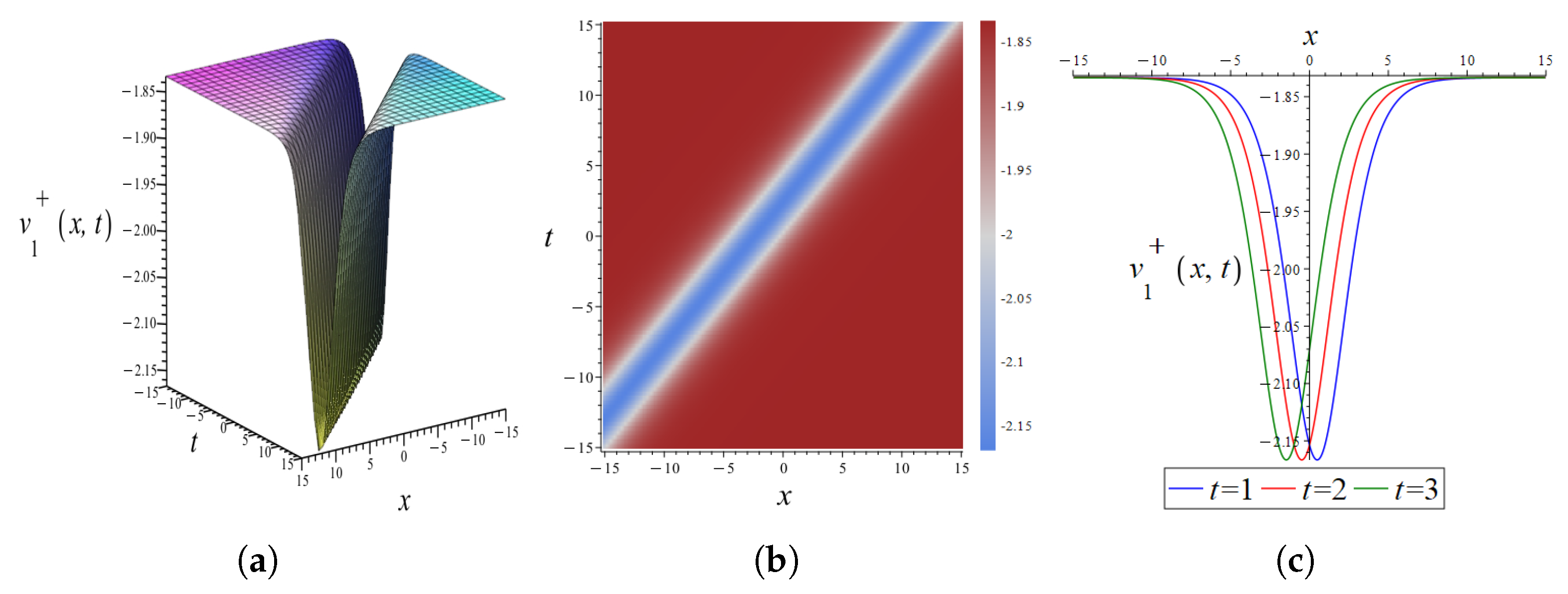
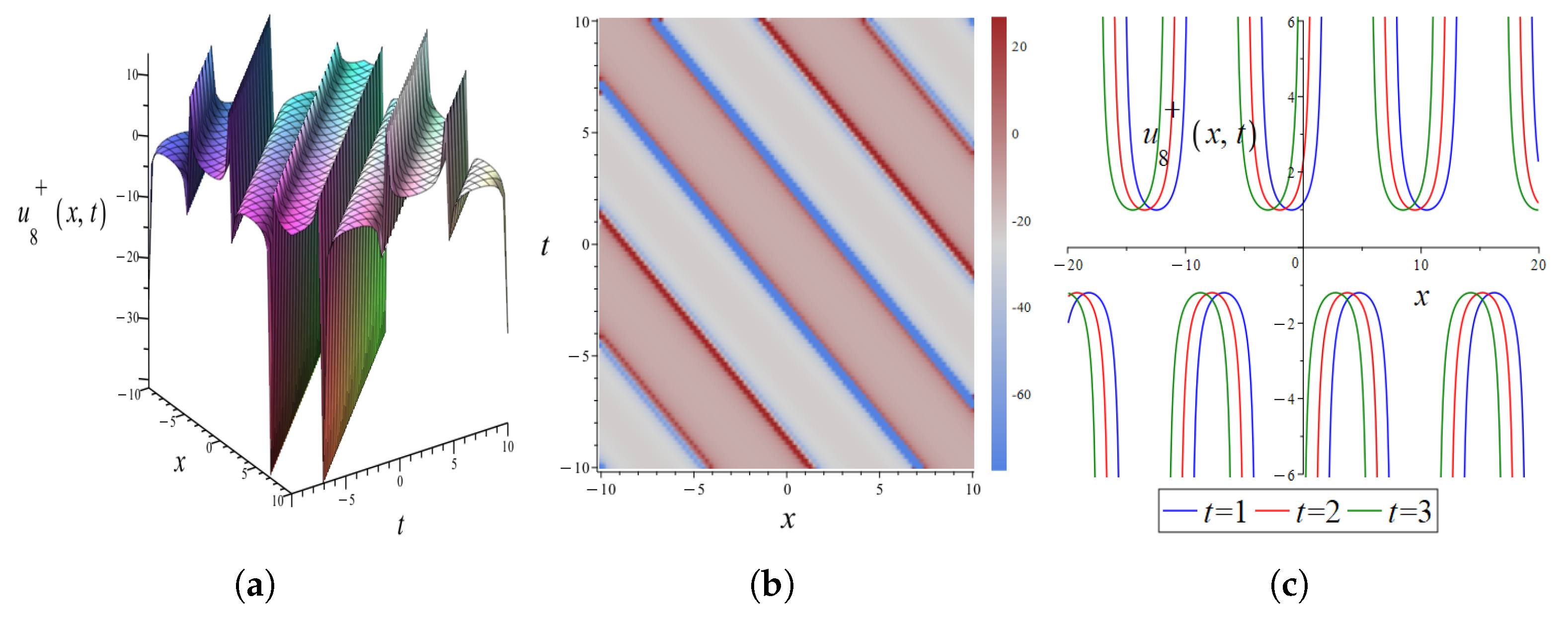
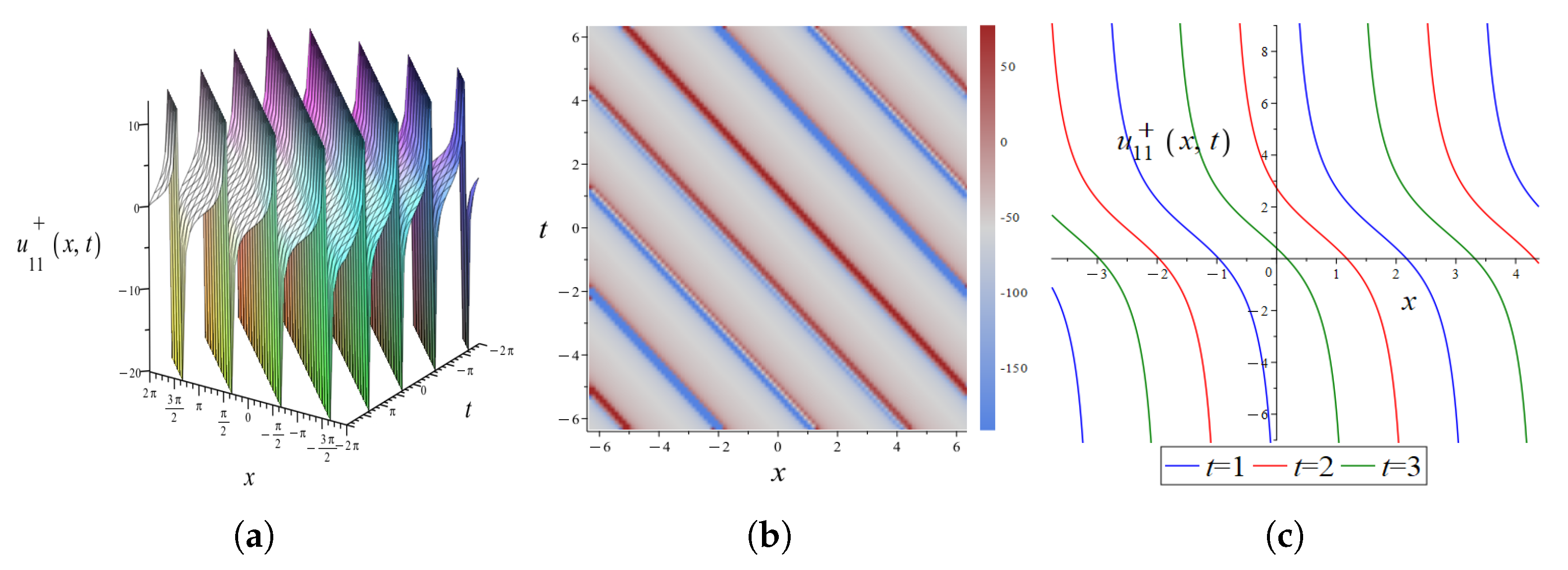
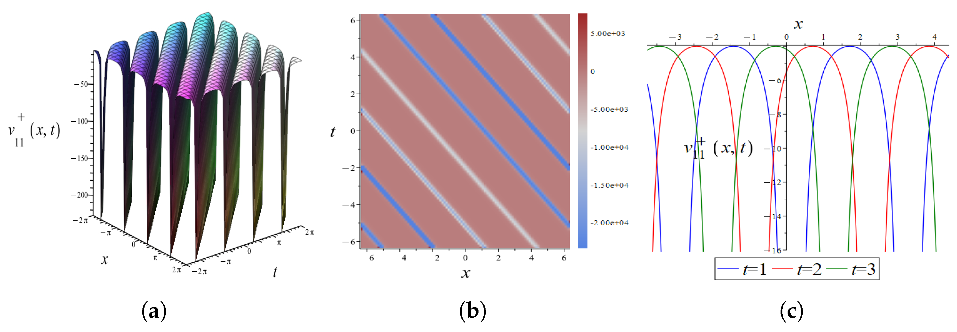
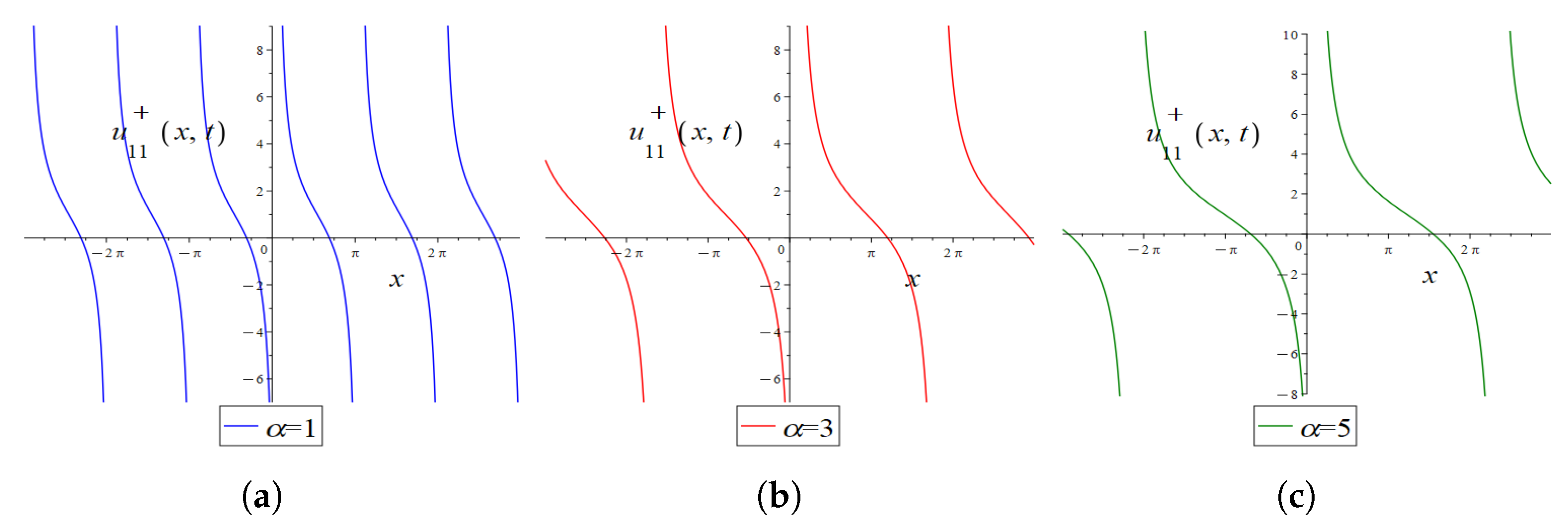
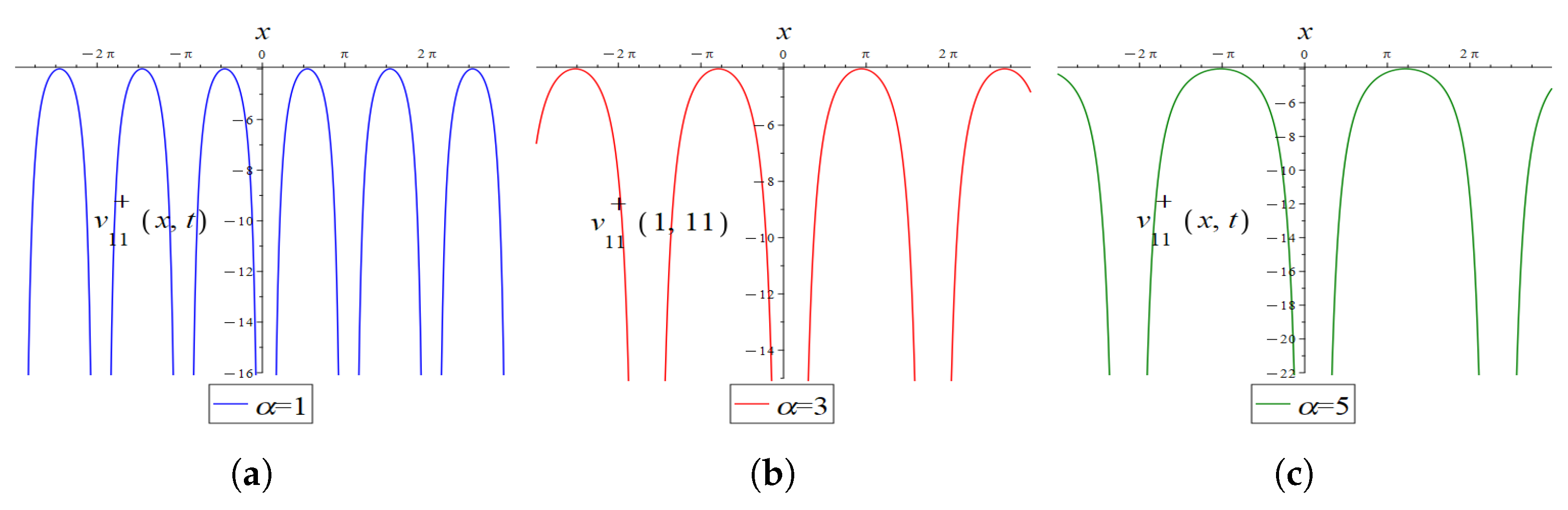
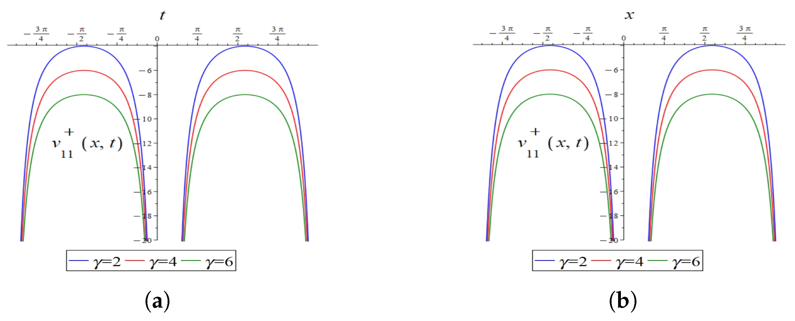
4.3. Graphical Interpretation of the Exact Solutions

Using the MSSM, we derive a wide range of solutions for gBBKW Equation (1) with $\beta =0$. For example, Case 1–Case 3 represent hyperbolic function solutions, Case 4–Case 5 correspond to trigonometric function solutions, Case 6 describes exponential function solutions, and Case 7 provides a rational function solution. To offer a more intuitive understanding of these exact solutions, three-dimensional, two-dimensional, and density plots are presented in Figures below. Two- and three-dimensional plots illustrate the evolution of waveforms over time and space, while also showing their propagation stability. Density plots reveal the intricate topological features of the solutions. The physical significance and characteristics of the depicted solutions are elaborated below.

(1) The parameters in Equation (58) were chosen as $\alpha =-1,\gamma =2,m_0=0.2,$$n_2=-1,s_1=1,s_2=-3,b_0=2$, and $\lambda =1$. This yields the bright soliton solution $u_1^{+}(x,t)$ and the dark soliton solution $v_1^{+}(x,t)$, as illustrated in Figure 13 and Figure 14. The bright soliton solution is characterized by a central maximum peak, whereas the dark soliton solution features a central minimum peak.

In comparing Figure 13 and Figure 14, it can be found that the wave exhibit the following characteristics:

(i) For the same time, as the wave velocity gradually reaches the maximum peak, the wave height gradually reaches the minimum peak. The position where wave velocity reaches its maximum precisely coincides with the position where wave height attains its minimum.

(ii) Wave velocity increases as wave height decreases. This phenomenon occurs because a reduction in wave height corresponds to an increase in wavelength, which in turn leads to an increase in wave velocity. The features depicted in the figures align with the characteristic behavior of shallow water waves.

(2) The parameters in Equation (59) were chosen as $\alpha =1,\gamma =2,m_0=0.4,$$n_2=-1,s_1=-2.6,s_2=0.8,b_0=0.32$, and $\lambda =1$. This yields the kink solution $u_4^{+}(x,t)$ and the bright soliton solution $v_4^{+}(x,t)$, as illustrated in Figure 15 and Figure 16. Kink solutions are widely applied in optics, fluid dynamics, and condensed matter physics. The kink solutions we obtained provide a mathematical description for simulating complex wave phenomena in fields such as fluid flow, nonlinear optics, and condensed matter physics using the gBBKW equations. For example, in optics, kink solutions can describe the propagation of light in nonlinear media. In fluid dynamics, they may associate with vortices and soliton waves.

In comparing Figure 15 and Figure 16, the following can be observed: (i) For the same time, the positions where the wave velocity and height change exhibit consistency. (ii) The position where wave velocity changes the most corresponds to the highest point of the wave height. As stated earlier, regions where wave velocity changes most noticeably often correspond to the peaks or troughs of shallow water waves. Figure 1 and Figure 2 illustrate the scenario where the point of fastest wave velocity change aligns with the wave trough. In contrast, Figure 15 and Figure 16 depict the situation where the point of fastest wave velocity change corresponds to the wave crest.

(3) The parameters in Equation (60) were chosen as $\alpha =1,\gamma =2,m_0=-0.1,n_2=-1,s_1=-0.3,s_2=0.5,b_0=10$, and $\lambda =-0.0003$. This yields the singular periodic wave solutions $u_8^{+}(x,t)$ and $v_8^{+}(x,t)$, as illustrated in Figure 17 and Figure 18. Figure 17c and Figure 18c provide a more intuitive representation of the periodic characteristics of the solutions. The periods depend on factors such as water depth and the type of fluctuation. The locations where wave velocity exhibits singularities coincide with those where wave height displays singularities. The singular points in the solutions may represent points of high energy concentration or vortices in the fluid. These points can interact with the periodic components of the wave, which can lead to complex motion patterns.

(4) The parameters in Equation (61) were chosen as $\alpha =1,\gamma =2,m_0=1,n_2=-2,s_1=2,s_2=1,b_0=-1$, and $\lambda =2$. This yields the periodic wave solution $u_{11}^{+}(x,t)$ and the dark periodic singular soliton solution $v_{11}^{+}(x,t)$, as illustrated in Figure 19 and Figure 20. Periodic wave solutions provide an important theoretical basis for understanding and controlling wave phenomena in oceanic environments. By analyzing the properties of periodic waves, we can improve predictions of ocean wave behavior and mitigate potential disasters. Dark periodic singular soliton solutions are particularly useful for describing certain characteristics of surface waves in the ocean. They may also aid in understanding and predicting extreme wave events, such as giant waves or tsunamis.

We further investigate the influence of variations in the diffusion power parameters on the periodicity of wave velocity and wave height.

(i) The impact of parameter $\alpha$ on the wave. Choose $t=1$ and substitute different values of $\alpha$ into Equation (61). The other parameters are the same as those selected in Figure 19 and Figure 20. Two-dimensional plots of $u_{11}^{+}(x,t)$ and $v_{11}^{+}(x,t)$ under different conditions of $\alpha$ are presented in Figure 21 and Figure 22. From these figures, it can be intuitively seen that as $\alpha$ increases, the period of spatial variation in wave velocity and height also increases.

(ii) The impact of parameter $\gamma$ on the wave. It is observed that $u_{11}^{+}(x,t)$ is not related to $\gamma$, whereas $v_{11}^{+}(x,t)$ is related to $\gamma$ through Equation (61). Choose $x=1$ and substitute different values of $\gamma$ into (61). The other parameters are the same as those selected in Figure 19 and Figure 20. Two-dimensional plots of $v_{11}^{+}(x,t)$ as a function of t under varying $\gamma$ conditions are presented in Figure 23a. These figures demonstrate that as $\gamma$ increases, the peak of wave height decreases, while the period remains unchanged. Choose $t=1$ and substitute different values of $\gamma$ into (61). Two-dimensional plots of $v_{11}^{+}(x,t)$ as a function of x under varying $\gamma$ conditions are shown in Figure 23b. The variations in wave height with respect to x exhibit characteristics similar to those with respect to t.

(5) The parameters in Equation (62) were chosen as $\alpha =1,\gamma =2,m_0=-1,n_2=-2,s_1=2,s_2=1,b_0=1$, and $\lambda =1$. This yields the singular solitary wave solution $u_{16}^{+}(x,t)$ and the singular soliton solution $v_{16}^{+}(x,t)$, as illustrated in Figure 24 and Figure 25.

The singular solitary wave solution can be used to describe the dynamic behavior of waves before and after breaking in shallow water. In the context of wave breaking, the singular solutions can be applied in the determination of critical point of wave breaking and the description of nonlinear dynamic behavior during the wave breaking process. The singular solitary wave can reflect extreme behaviors in a system, such as shock waves and localized high-energy events. These solutions describe the propagation characteristics of water waves with discontinuous profiles or sharp peaks, offering a mathematical tool for modeling complex wave phenomena that cannot be adequately represented by smooth wave solutions.

5. Conclusions

We derive a variety of novel solutions for gBBKW equations using a combination of methods. As an important nonlinear equation describing certain gravity water waves in a shallow-ocean scenario, the exact solutions of the gBBKW equations provide us with a tool for a deeper understanding of ocean wave phenomena. For instance, in both one-soliton and multi-soliton solutions, the positions where wave velocity and height change exhibit consistency, reflecting the characteristic behavior of shallow water waves. In bright and dark soliton solutions, the position of the wave peak for the wave velocity of the bright soliton exactly corresponds to the position of the wave trough for the wave height of the dark soliton. This accurately demonstrates the characteristic while the wave velocity increases as wave height decreases in shallow water waves. Singular periodic solutions may help understand and predict extreme wave events, such as giant waves or tsunamis. And a singular solitary wave solution can help describe the propagation characteristics of waves, while the wave profiles exhibit sharp features or rapid changes.

These exact solutions provide a precise description of variations in wave velocity and wave height, which can help us understand the propagation characteristics of waves in shallow waters, including changes in wave speed, wavelength, and wave height. They are useful as a guide toward obtaining numerical solutions or performing simulations. The study of the gBBKW equations provides a theoretical basis for revealing the internal physical mechanisms of wave systems. This research has practical implications for predicting wave impacts on coastlines, ensuring ship navigation safety, and designing marine structures. The ratio of wave height to wave velocity obtained from the exact solutions has potential applications in engineering design and scientific research. Future studies may explore the geometric foundations [1] of the gBBKW equations to characterize multi-soliton dynamics. The other forms of nonclassical symmetries and high-dimensional gBBKW systems deserve to be further studied.

References

1. Kodama, Y. KP Solitons and the Grassmannians; Springer Briefs in Mathematical Physics; Springer: Singapore, 2017. [Google Scholar]
2. Maleewong, M.; Grimshaw, R. Evolution of wind-generated shallow-water waves in the framework of a modified Kadomtsev-Petviashvili equation. Fluids 2025, 10, 61. [Google Scholar] [CrossRef]
3. Thomas, D.B. Cosmological gravity on all scales: Simple equations, required conditions, and a framework for modified gravity. Phys. Rev. D 2020, 101, 123517. [Google Scholar] [CrossRef]
4. Bernardo, H.; Franzmann, G. α-Cosmology: Solutions and stability analysis. J. High Energy Phys. 2020, 2020, 1–15. [Google Scholar] [CrossRef]
5. Joseph, G.W.; Övgün, A. Cosmology with variable G and nonlinear electrodynamics. Indian J. Phys. 2022, 96, 1861–1866. [Google Scholar] [CrossRef]
6. Vasiliev, M.A. Nonlinear equations for symmetric massless higher spin fields in (A)dSd. Phys. Lett. B 2003, 567, 139–151. [Google Scholar] [CrossRef]
7. Benci, V.; Fortunato, D. Variational Methods in Nonlinear Field Equations; Springer: Berlin/Heidelberg, Germany, 2014. [Google Scholar]
8. Cheemaa, N.; Seadawy, A.R.; Sugati, T.G.; Baleanu, D. Study of the dynamical nonlinear modified Korteweg–de Vries equation arising in plasma physics and its analytical wave solutions. Results Phys. 2020, 19, 103480. [Google Scholar] [CrossRef]
9. El-Tantawy, S.A.; Salas, A.H.; Alyousef, H.A.; Alharthi, M.R. Novel exact and approximate solutions to the family of the forced damped Kawahara equation and modeling strong nonlinear waves in a plasma. Chin. J. Phys. 2022, 77, 2454–2471. [Google Scholar] [CrossRef]
10. Xie, X.Y.; Meng, G.Q. Collisions between the dark solitons for a nonlinear system in the geophysical fluid. Chaos Soliton. Fract. 2018, 107, 143–145. [Google Scholar] [CrossRef]
11. Panoiu, N.C.; Sha, W.E.I.; Lei, D.Y.; Li, G.C. Nonlinear optics in plasmonic nanostructures. J. Opt. 2018, 20, 083001. [Google Scholar] [CrossRef]
12. Wen, X.; Gong, Z.; Li, D. Nonlinear optics of two-dimensional transition metal dichalcogenides. InfoMat 2019, 1, 317–337. [Google Scholar] [CrossRef]
13. Johnson, R.S. Application of the ideas and techniques of classical fluid mechanics to some problems in physical oceanography. Philos. Trans. R. Soc. A 2018, 376, 20170092. [Google Scholar] [CrossRef]
14. Wang, H.F.; Zhang, Y.F. Residual symmetries and Bäcklund transformations of (2+1)-dimensional strongly coupled Burgers system. Adv. Math. Phys. 2020, 2020, 6821690. [Google Scholar] [CrossRef]
15. Malik, S.; Almusawa, H.; Kumar, S.; Wazwaz, A.M.; Osman, M.S. A (2+1)-dimensional Kadomtsev–Petviashvili equation with competing dispersion effect: Painlevé analysis, dynamical behavior and invariant solutions. Results Phys. 2021, 23, 104043. [Google Scholar] [CrossRef]
16. Rizvi, S.T.R.; Seadawy, A.R.; Younis, M.; Ali, I.; Althobaiti, S.; Mahmoud, S.F. Soliton solutions, Painleve analysis and conservation laws for a nonlinear evolution equation. Results Phys. 2021, 23, 103999. [Google Scholar] [CrossRef]
17. Yuan, F.; He, J.S.; Cheng, Y. Exact solutions of a (2+1)-dimensional extended shallow water wave equation. Chinese Phys. B 2019, 28, 237–244. [Google Scholar] [CrossRef]
18. Zhang, Z.; Li, B.; Chen, J.; Guo, Q. Construction of higher-order smooth positons and breather positons via Hirota’s bilinear method. Nonlinear Dynam. 2021, 105, 2611–2618. [Google Scholar] [CrossRef]
19. Zhang, G.; Yan, Z. The derivative nonlinear Schrödinger equation with zero/nonzero boundary conditions: Inverse scattering transforms and N-double-pole solutions. J. Nonlinear Sci. 2020, 30, 3089–3127. [Google Scholar] [CrossRef]
20. Xin, X.; Liu, Y.; Xia, Y.; Liu, H. Integrability, Darboux transformation and exact solutions for nonlocal couplings of AKNS equations. Appl. Math. Lett. 2021, 119, 107209. [Google Scholar] [CrossRef]
21. Wang, X.; He, J.S. Darboux transformation and general soliton solutions for the reverse space-time nonlocal short pulse equation. Phys. D 2023, 446, 133639. [Google Scholar] [CrossRef]
22. Wang, H.F.; Zhang, Y.F. A kind of nonisospectral and isospectral integrable couplings and their Hamiltonian systems. Commun. Nonlinear Sci. 2021, 99, 105822. [Google Scholar] [CrossRef]
23. Liu, W.H.; Zhang, Y.F. Optimal systems, similarity reductions and new conservation laws for the classical Boussinesq–Burgers system. Eur. Phys. J. Plus 2020, 135, 1–11. [Google Scholar] [CrossRef]
24. Benoudina, N.; Zhang, Y.; Khalique, C.M. Lie symmetry analysis, optimal system, new solitary wave solutions and conservation laws of the Pavlov equation. Commun. Nonlinear Sci. 2021, 94, 105560. [Google Scholar] [CrossRef]
25. Wang, H.F.; Zhang, Y.F. Application of Riemann–Hilbert method to an extended coupled nonlinear Schrödinger equations. Comput. Appl. Math. 2023, 420, 114812. [Google Scholar] [CrossRef]
26. Wu, J. Riemann–Hilbert approach and soliton analysis of a novel nonlocal reverse-time nonlinear Schrödinger equation. Nonlinear Dynam. 2024, 112, 4749–4760. [Google Scholar] [CrossRef]
27. Yin, Y.H.; Lü, X.; Ma, W.X. Bäcklund transformation, exact solutions and diverse interaction phenomena to a (3+1)-dimensional nonlinear evolution equation. Nonlinear Dynam. 2022, 108, 4181–4194. [Google Scholar] [CrossRef]
28. Dong, S.; Lan, Z.Z.; Gao, B.; Shen, Y.J. Bäcklund transformation and multi-soliton solutions for the discrete Korteweg–de Vries equation. Appl. Math. Lett. 2022, 125, 107747. [Google Scholar] [CrossRef]
29. Lou, S.Y. Residual symmetries and Bäcklund transformations. arXiv 2013, arXiv:1308.1140. [Google Scholar]
30. Lou, S.Y. Consistent Riccati expansion and solvability. arXiv 2013, arXiv:1308.5891. [Google Scholar]
31. Lou, S.Y. Consistent Riccati expansion for integrable systems. Stud. Appl. Math. 2015, 134, 372–402. [Google Scholar] [CrossRef]
32. Ren, B.; Lin, J. Soliton molecules, nonlocal symmetry and CRE method of the KdV equation with higher-order corrections. Phys. Scr. 2020, 95, 075202. [Google Scholar] [CrossRef]
33. Song, J.F.; Hu, Y.H.; Ma, Z.Y. Bäcklund transformation and CRE solvability for the negative-order modified KdV equation. Nonlinear Dynam. 2017, 90, 575–580. [Google Scholar] [CrossRef]
34. Ren, B.; Lin, J.; Liu, P. Soliton molecules and the CRE method in the extended mKdV equation. Commun. Theor. Phys. 2020, 72, 55005. [Google Scholar] [CrossRef]
35. Liu, P.; Cheng, J.; Ren, B.; Yang, J.R. Bäcklund transformations, consistent Riccati expansion solvability, and soliton–cnoidal interaction wave solutions of Kadomtsev–Petviashvili equation. Chin. Phys. B 2020, 29, 020201. [Google Scholar] [CrossRef]
36. Sheng, Q.; Wo, W. Symmetry analysis and interaction solutions for the (2+1)-dimensional Kaup–Kupershmidt system. Appl. Math. Lett. 2016, 58, 165–171. [Google Scholar] [CrossRef]
37. Liu, X.Z.; Yu, J.; Lou, Z.M.; Cao, Q.J. Residual symmetry reduction and consistent Riccati expansion of the generalized kaup-kupershmidt equation. Commun. Theor. Phys. 2016, 69, 625–630. [Google Scholar] [CrossRef]
38. Cheng, W.; Li, B. CRE Solvability, Exact Soliton-Cnoidal Wave Interaction Solutions, and Nonlocal Symmetry for the Modified Boussinesq Equation. Adv. Math. Phys. 2016, 2016, 4874392. [Google Scholar] [CrossRef]
39. Zhao, Z.; Han, B. Nonlocal symmetry and explicit solutions from the CRE method of the Boussinesq equation. Eur. Phys. J. Plus 2018, 133, 1–9. [Google Scholar] [CrossRef]
40. Rezazadeh, H.; Inc, M.; Baleanu, D. New solitary wave solutions for variants of (3+1)-dimensional Wazwaz-Benjamin-Bona-Mahony equations. Front. Phys. 2020, 8, 332. [Google Scholar] [CrossRef]
41. Akinyemi, L.; Akpan, U.; Veeresha, P.; Rezazadeh, H.; Inc, M. Computational techniques to study the dynamics of generalized unstable nonlinear Schrödinger equation. J. Ocean Eng. Sci. 2022. [Google Scholar] [CrossRef]
42. Murad, M.A.S.; Ismael, H.F.; Sulaiman, T.A. Various exact solutions to the time-fractional nonlinear Schrödinger equation via the new modified Sardar sub-equation method. Phys. Scr. 2024, 99, 085252. [Google Scholar] [CrossRef]
43. Ahmad, J.; Hameed, M.; Mustafa, Z.; Rehman, S.U. Soliton patterns in the truncated M-fractional resonant nonlinear Schrödinger equation via modified Sardar sub-equation method. J. Opt. 2024, 1–22. [Google Scholar] [CrossRef]
44. Kamel, N.M.; Ahmed, H.M.; Rabie, W.B. Retrieval of soliton solutions for 4th-order (2+1)-dimensional Schrödinger equation with higher-order odd and even terms by modified Sardar sub-equation method. Ain. Shams. Eng. J. 2024, 15, 102808. [Google Scholar] [CrossRef]
45. Hamid, I.; Kumar, S. Newly formed solitary wave solutions and other solitons to the (3+1)-dimensional mKdV–ZK equation utilizing a new modified Sardar sub-equation approach. Mod. Phys. Lett. B 2024, 39, 2550027. [Google Scholar] [CrossRef]
46. Gao, X.Y.; Guo, Y.J.; Shan, W.R. Ocean shallow-water studies on a generalized Boussinesq-Broer-Kaup-Whitham system: Painlevé analysis and similarity reductions. Chaos Soliton. Fract. 2023, 169, 113214. [Google Scholar] [CrossRef]
47. Fan, E. Multiple travelling wave solutions of nonlinear evolution equations using a unified algebraic method. J. Phys. A 2002, 35, 6853. [Google Scholar] [CrossRef]
48. Bhrawy, A.H.; Tharwat, M.M.; Abdelkawy, M.A. Integrable system modelling shallow water waves: Kaup–Boussinesq shallow water system. Indian J. Phys. 2013, 87, 665–671. [Google Scholar] [CrossRef]
49. Congy, T.; Ivanov, S.K.; Kamchatnov, A.M.; Pavloff, N. Evolution of initial discontinuities in the Riemann problem for the Kaup-Boussinesq equation with positive dispersion. Chaos 2017, 27, 083107. [Google Scholar] [CrossRef]
50. Wei, L.; Ding, X.F. Using symbolic computation to construct travelling wave solutions to nonlinear partial differential equations. Chin. Phys. 2004, 13, 1639. [Google Scholar] [CrossRef]
51. Wang, Y.; Gao, B. Non-local symmetry, interaction solutions and conservation laws of the (1+1)-dimensional Wu-Zhang equation. Pramana-J. Phys. 2021, 95, 129. [Google Scholar] [CrossRef]
52. Fan, E.; Hon, Y.C. A series of travelling wave solutions for two variant Boussinesq equations in shallow water waves. Chaos Soliton. Fract. 2003, 15, 559–566. [Google Scholar] [CrossRef]
53. Singh, K.; Gupta, R.K. Exact solutions of a variant Boussinesq system. Int. J. Eng. Sci. 2006, 44, 1256–1268. [Google Scholar] [CrossRef]
54. Fei, J.; Ma, Z.; Cao, W. Residual symmetries and interaction solutions for the Whitham-Broer-Kaup equation. Nonlinear Dynam. 2017, 88, 395–402. [Google Scholar] [CrossRef]
55. Wang, K.J.; Wang, K.L. Variational principles for fractal Whitham–Broer–Kaup equations in shallow water. Fractals 2021, 29, 2150028. [Google Scholar] [CrossRef]
56. Kupershmidt, B.A. Mathematics of dispersive water waves. Commun. Math. Phys. 1985, 99, 51–73. [Google Scholar] [CrossRef]
57. Li, Y.; Zhang, J.E. Darboux transformations of classical Boussinesq system and its multi-soliton solutions. Phys. Lett. A 2001, 284, 253–258. [Google Scholar] [CrossRef]
58. Rahioui, M.; El Kinani, E.H.; Ouhadan, A. Nonlocal residual symmetries, N-th Bäcklund transformations and exact interaction solutions for a generalized Broer–Kaup–Kupershmidt system. Z. Angew. Math. Phys. 2024, 75, 37. [Google Scholar] [CrossRef]
59. Olver, P.J. Applications of Lie Groups to Differential Equations; Springer: Berlin/Heidelberg, Germany, 1993. [Google Scholar]
60. Zhao, Z.; Han, B. Residual symmetry, Bäcklund transformation and CRE solvability of a (2+1)-dimensional nonlinear system. Nonlinear Dynam. 2018, 94, 461–474. [Google Scholar] [CrossRef]
61. Liu, Y.; Li, B. Nonlocal symmetry and exact solutions of the (2+1)-dimensional Gardner equation. Chin. J. Phys. 2016, 54, 718–723. [Google Scholar] [CrossRef]
Figure 1. (a) Three-dimensional plot of kink solution u in Equation (23). (b) Two-dimensional plot of kink solution u( t = 1 , 2 , 3 ).
Fractalfract 09 00305 g001
Figure 2. (a) Three-dimensional plot of dark one-soliton solution v in Equation (23). (b) Two-dimensional plot of dark one-soliton solution v( t = 1 , 2 , 3 ).
Fractalfract 09 00305 g002
Figure 3. (a) Spatial evolution of u in Equation (23) under different parameter values of α . (b) Spatial evolution of v in Equation (23) under different parameter values of α .
Fractalfract 09 00305 g003
Figure 4. (a) Spatial evolution of u in (23) with β = 0.9 , 0.8 . (b) Spatial evolution of u in (23) with β = 0.8 , 0.9 . (c) Spatial evolution of v in (23) with different β .
Fractalfract 09 00305 g004
Figure 5. Two-kink solution of u in Equation (27) ( N = 2 ). (a) Three-dimensional plot of u. (b) The density plot of u. (c) Two-dimensional plot of u( t = 9 , 12 , 15 ).
Fractalfract 09 00305 g005
Figure 6. Two-soliton solution of v in Equation (28) ( N = 2 ). (a) Three-dimensional plot of v. (b) The density plot of v. (c) Two-dimensional plot of v( t = 9 , 12 , 15 ).
Fractalfract 09 00305 g006
Figure 7. Three-kink solution of u in Equation (27) ( N = 3 ). (a) Three-dimensional plot of u. (b) The density plot of u. (c) Two-dimensional plot of u( t = 15 , 18 , 21 ).
Fractalfract 09 00305 g007
Figure 8. Three-soliton solution of v in Equation (28) ( N = 3 ). (a) Three-dimensional plot of v. (b) The density plot of v. (c) Two-dimensional plot of v( t = 15 , 18 , 21 ).
Fractalfract 09 00305 g008
Figure 9. (a) Three-dimensional plot of anti-kink solution u in Equation (39). (b) Two-dimensional plot of anti-kink solution u( t = 1 , 5 , 9 ).
Fractalfract 09 00305 g009
Figure 10. (a) Three-dimensional plot of bright soliton solution v in Equation (39). (b) Two-dimensional plot of bright soliton solution v( t = 1 , 5 , 9 ).
Fractalfract 09 00305 g010
Figure 11. Soliton–cnoidal wave u ( x , t ) in Equation (46). (a) Three-dimensional wave plot of u ( x , t ) . (b) The density plot of u ( x , t ) . (c) The wave u ( x , 1 ) along the x axis.
Fractalfract 09 00305 g011
Figure 12. Soliton–cnoidal wave v ( x , t ) in Equation (47). (a) Three-dimensional wave plot of v ( x , t ) . (b) The density plot of v ( x , t ) . (c) The wave v ( x , 1 ) along the x axis.
Fractalfract 09 00305 g012
Figure 13. (a) Three-dimensional plot of bright soliton solution u 1 + ( x , t ) in Equation (58). (b) The density plot of bright soliton solution u 1 + ( x , t ) . (c) Two-dimensional plot of bright soliton solution u 1 + ( x , t ) ( t = 1 , 2 , 3 ).
Fractalfract 09 00305 g013
Figure 14. (a) Three-dimensional plot of dark soliton solution v 1 + ( x , t ) in Equation (58). (b) The density plot of dark soliton solution v 1 + ( x , t ) . (c) Two-dimensional plot of dark soliton solution v 1 + ( x , t ) ( t = 1 , 2 , 3 ).
Fractalfract 09 00305 g014
Figure 15. (a) Three-dimensional plot of kink solution u 4 + ( x , t ) in Equation (59). (b) The density plot of kink solution u 4 + ( x , t ) . (c) Two-dimensional plot of kink solution u 4 + ( x , t ) ( t = 1 , 5 , 9 ).
Fractalfract 09 00305 g015
Figure 16. (a) Three-dimensional plot of bright soliton solution v 4 + ( x , t ) in Equation (59). (b) The density plot of bright soliton solution v 4 + ( x , t ) . (c) Two-dimensional plot of bright soliton solution v 4 + ( x , t ) ( t = 1 , 5 , 9 ).
Fractalfract 09 00305 g016
Figure 17. (a) Three-dimensional plot of singular periodic wave solution u 8 + ( x , t ) in Equation (60). (b) The density plot of singular periodic wave solution u 8 + ( x , t ) . (c) Two-dimensional plot of singular periodic wave solution u 8 + ( x , t ) ( t = 1 , 2 , 3 ).
Fractalfract 09 00305 g017
Figure 18. (a) Three-dimensional plot of singular periodic wave solution v 8 + ( x , t ) in Equation (60). (b) The density plot of singular periodic wave solution v 8 + ( x , t ) . (c) Two-dimensional plot of singular periodic wave solution v 8 + ( x , t ) ( t = 1 , 2 , 3 ).
Fractalfract 09 00305 g018
Figure 19. (a) Three-dimensional plot of periodic wave solution u 11 + ( x , t ) in Equation (61). (b) The density plot of periodic wave solution u 11 + ( x , t ) . (c) Two-dimensional plot of periodic wave solution u 11 + ( x , t ) ( t = 1 , 2 , 3 ).
Fractalfract 09 00305 g019
Figure 20. (a) Three-dimensional plot of dark periodic singular soliton solution v 11 + ( x , t ) in Equation (61). (b) The density plot of dark periodic singular soliton solution v 11 + ( x , t ) . (c) Two-dimensional plot of dark periodic singular soliton solution v 11 + ( x , t ) ( t = 1 , 2 , 3 ).
Fractalfract 09 00305 g020
Figure 21. u 11 + ( x , t ) with (a) α = 1 , (b) α = 3 , (c) α = 5 .
Fractalfract 09 00305 g021
Figure 22. v 11 + ( x , t ) with (a) α = 1 , (b) α = 3 , (c) α = 5 .
Fractalfract 09 00305 g022
Figure 23. (a) v 11 + ( x , t ) regarding t with γ = 2 , 4 , 6 . (b) v 11 + ( x , t ) regarding x with γ = 2 , 4 , 6 .
Fractalfract 09 00305 g023
Figure 24. (a) Three-dimensional plot of singular solitary wave solution u 16 + ( x , t ) in Equation (62). (b) The density plot of singular solitary wave solution u 16 + ( x , t ) . (c) Two-dimensional plot of singular solitary wave solution u 16 + ( x , t ) ( t = 1 , 2 , 3 ).
Fractalfract 09 00305 g024
Figure 25. (a) Three-dimensional plot of singular soliton solution v 16 + ( x , t ) in Equation (62). (b) The density plot of singular soliton solution v 16 + ( x , t ) . (c) Two-dimensional plot of singular soliton solution v 16 + ( x , t ) ( t = 1 , 2 , 3 ).
Fractalfract 09 00305 g025
Disclaimer/Publisher’s Note: The statements, opinions and data contained in all publications are solely those of the individual author(s) and contributor(s) and not of MDPI and/or the editor(s). MDPI and/or the editor(s) disclaim responsibility for any injury to people or property resulting from any ideas, methods, instructions or products referred to in the content.