Design of Non-Standard Finite Difference and Dynamical Consistent Approximation of Campylobacteriosis Epidemic Model with Memory Effects

Abstract

Campylobacteriosis has been described as an ever-changing disease and health issue that is rather dangerous for different population groups all over the globe. The World Health Organization (WHO) reports that 33 million years of healthy living are lost annually, and nearly one in ten persons have foodborne illnesses, including Campylobacteriosis. This explains why there is a need to develop new policies and strategies in the management of diseases at the intergovernmental level. Within this framework, an advanced stochastic fractional delayed model for Campylobacteriosis includes new stochastic, memory, and time delay factors. This model adopts a numerical computational technique called the Grunwald–Letnikov-based Nonstandard Finite Difference (GL-NSFD) scheme, which yields an exponential fitted solution that is non-negative and uniformly bounded, which are essential characteristics when working with compartmental models in epidemic research. Two equilibrium states are identified: the first is an infectious Campylobacteriosis-free state, and the second is a Campylobacteriosis-present state. When stability analysis with the help of the basic reproduction number $R_0$ is performed, the stability of both equilibrium points depends on the $R_0$ value. This is in concordance with the actual epidemiological data and the research conducted by the WHO in recent years, with a focus on the tendency to increase the rate of infections and the necessity to intervene in time. The model goes further to analyze how a delay in response affects the band of Campylobacteriosis spread, and also agrees that a delay in response is a significant factor. The first simulations of the current state of the system suggest that certain conditions can be achieved, and the eradication of the disease is possible if specific precautions are taken. The outcomes also indicate that enhancing the levels of compliance with the WHO-endorsed SOPs by a significant margin can lower infection rates significantly, which can serve as a roadmap to respond to this public health threat. Unlike most analytical papers, this research contributes actual findings and provides useful recommendations for disease management approaches and policies.

1. Introduction

In [1], the authors presented a deterministic model for Campylobacteriosis, with an emphasis on zoonotic transmission, and compared different control measures to find the best control strategies. The model was intended to study the characteristics of the disease and assess the potential approaches to its control using vaccination, treatment, or environmental modification efforts. For the numerical calculations, the nonstandard finite difference (NSFD) scheme was used to analyze the accuracy and stability of the model through time. The above approach was useful in establishing how feasible it was to invest to minimize the prevalence of this disease. In [2], the authors concentrated on Campylobacteriosis, a common bacterial disease that is mediated by different species of Campylobacter, especially Campylobacter jejuni and Campylobacter coli. This infection is one of the most reported and mainly targets the gastrointestinal tract, with signs of diarrhea, abdominal pain, fever, and nausea being observed. It is commonly spread through ingesting contaminated food, the chief source being undercooked poultry, raw milk that has not been pasteurized, or water that has not been treated. More information is needed regarding the mode of transmission by which Campylobacter strains spread, the mechanisms by which these bacteria cause disease, and the possible ways to tackle and control this infection. In [3], the authors used the geographical approach, while the study differentiated the impact of certain weather parameters on the given seasonal factors and focused on Campylobacteriosis. Different weather conditions were analyzed to understand how they contribute the most to the spreading of this bacterial infection at different seasons. Such an approach made it possible to carry out a more systematic analysis of the effects of environmental factors on the occurrence of Campylobacteriosis. In [4], the authors suggested a novel mathematical model that could explain and encompass all of the multifaceted observations associated with Campylobacter jejuni biofilm development. As such, our strategy utilizes a discrete, probabilistic model based on a cellular automaton to model biofilm dynamics. It is crucial to note that the model includes the competence model of biofilm initiation, which deals with the likelihood of biofilm random start, particularly taking into consideration the environment and microbial flora, as well as the model of biofilm growth. This integration of the model gives an understanding of the factors of the formation of biofilm by C. jejuni, enhancing the understanding of this model of the formulation. In [5], the authors concentrated on the construction of mechanistically based complex predictive mathematical models for the adhesion and detachment of multiple species of biofilms. This involves also comprehending the relationships between microbial species, the environment into which the biofilm is to be formed or from which it has to be removed, and any other forces that might be involved. Thus, while modeling these dynamics, the study seeks to enhance the understanding of how to effectively manage biofilm formation in medical, industrial, and environmental applications. Finally, these types of models may help identify the processes that may help avoid the problems associated with biofilms and improve methods of cleaning and disinfection. In [6], the authors examined the distribution of phase variable genes in the Campylobacter jejuni clonal complexes and sought to reveal how these genes impact the adaptive potential among the bacterial strains. In [7], the authors conducted to determine the point prevalence of Campylobacter in a U.S. commercial broiler production farm system by simply observing the level of contamination at different stages. It also attempted to categorize the types of Campylobacter strains that are likely to be in the farm environment. This research is relevant to establish the trends of infection and then work on the recommended measures to be taken to enhance safety in food and general health. In [8], the authors discussed other possible ways of improving the management of CJ by employing a theragnostic concept. This includes the practice of using chicken embryos as the critical pre-clinical model to determine and enhance their ‘therapeutic and diagnostic approaches’. As a result of this integration, the anticipated benefit is the enhancement of the general CJ control and treatment effectiveness. In [9], the authors focused on the pathophysiological alterations of the GI tract following an infection with Campylobacter jejuni and explained how this bacterial infection impacts the functional and structural integrity of the gastrointestinal tract with emphasis on the processes that are involved. They analyzed changes in gut physiology, which entailed looking at inflammation and breach of the mucosal layer. In [10], the authors quantified the ability of asinex library compounds to bind to the Campylobacter jejuni DsbA1 protein, which is a core thiol-disulfide oxidoreductase enzyme that is used in the protein oxidation of bacterial pathogen proteins. Because the DsbA1 enzyme has a central role in bacterial virulence, it can be useful for the development of anti-viral compounds. This particular evaluation is therefore aimed at establishing, among other things, antiviral compounds that may interfere with this important enzymatic activity and reduce the pathogenicity of bacteria. In [11], the authors studied the indications of this bacterium in raw milk by both the quantitative and qualitative observations of colony-forming units (CFUs) and viable but non-culturable cells (VBNCs). This was regarded when determining the impact of these two different states on the bacterium’s survival and ability to persist in raw milk. In [12], the authors conducted a comprehensive comparison of three source attribution methodologies: Machine Learning, Network Analysis, and Bayesian modeling. They evaluated their performance using three distinct types of whole genome sequences (WGS) data inputs: the known typing schemas that can be used are core genome multi-locus sequence typing (cg MLST), 5-Mers, and 7-Mers. In effect, this analysis seeks to assess the validity of each approach in informing sources based on different types of genomic data. In [13], the authors studied some factors that lead to antimicrobial resistance in Campylobacter, emphasizing the need to supervise antimicrobial utilization in medical and farming fraternities. This research highlights the need to step up the surveillance and regulation mechanisms to counter this advance of resistance. Thus, the findings speak for the synergic approach of merging healthcare and agriculture into the common fight against antimicrobial-resistant pathogens that have become increasingly detrimental. In [14], authors proposed a new algorithm called ‘LPEM’ (Linear Programming-based Elementary Mode decomposition) that takes, from a steady-state flux value of a metabolic model—including genome-scale models—a unique vector and dissects it into several components, each of which corresponds to a weighted elementary mode. Indeed, these elementary modes are considered metabolic base flux modes, and LPEM guarantees that the weighted sum of these modes will correspond to the original flux vector. This approach allowed for reaching a high resolution at the pathway level to study the Metabolic network and its usage in using different pathways. In [15], the authors provided a systematic and up-to-date picture of the global burden of Campylobacteriosis, highlighting the importance of official actions in the control of the pathogen. The discussion showed how the infection happened by pointing out that the food handlers somehow contributed to the spread of the pathogen. Also, extraordinary emphasis was made on the aspect of food safety measures as a reason for controlling the spread and health preservation. In [16], the authors constructed detail-specific growth rate models for Campylobacter jejuni, Campylobacter coli, and Campylobacter growing in controlled pure culture environments. They determined the growth kinetics of the species in question: lag phase duration, specific growth rate, and maximum cell density. All of these measurements were carried out under comparable environmental settings to provide consistent comparisons of the growth attributes of every Campylobacter species. In [17], the authors aimed to identify the diagnostic performance of a range of assays for Campylobacter infection. In particular, by combining data from several sources, they aimed to assess the reliability and efficacy of the above diagnostic tools. The evidence synthesis offers a clear assessment of the extent to which these tests performed in the detection of Campylobacter across settings and populations. In [18], the authors studied naturally occurring Campylobacter-associated diarrhea in Indian rhesus macaques to assess the impact of vaccination in reducing severe diarrheal disease and growth stunting in infants. This research was intended to find out more information on how vaccination could be used as an intervention in preventing the degree and effects of Campylobacter infections. The study offers information for future practicable measures of enhancing the well-being of both primates and humans who suffer from comparable illnesses. Muthukrishnan et al. [19] studied the time variability of Campylobacter spp. Its density and presence were assessed in different camels. In several matrices, cows’ milk, feces, surfaces of the farm, and teat skin throughout a year on a dairy farm in Germany. For this extensive survey, we aim to examine the effects of seasonality and environment on bacterial density and distribution and examine how any of these may affect the dairy farm hygiene and animal health in several weeks of the year. In [20], the authors outlined key areas that needed more focus to gain further Campylobacter reduction in poultry meat. It is also important to set a standard measure that would be used in the assessment of these interventions. It should be used as a reference point for easy comparisons and enhancements of future strategies of Campylobacter control.

The stochastic delayed method consequently combines stochastic processes, fractional calculus, and temporal delays as its powerful apparatus for a better representation of the complexity of the real world. This approach goes further, using the memory effects that are incorporated by fractional derivatives, which are vital in fields like biology and economics, where past events determine the current and future events. By including delay, this method can simulate the time in between cause and effect, hence making the system representations realistic. The stochastic component looks into the inherent elements of risks and probability within such systems to enhance the modeling of the uncertainties. Altogether, these elements enhance the elaboration of more precise models regarding reality and improve the comprehension of different real processes in practically all scientific branches.

Based on the structure of this paper, seven sections have been created to ensure that major areas of Campylobacteriosis dynamics are tackled effectively. In Section 1, a general background is provided with a literature review of the disease and its infection rates comparable to other infectious diseases, namely Campylobacteriosis. This section, therefore, lays some background by providing the previous works and theoretical literature related to the present research study. Section 2 expands on the delayed model by presenting the stochastic fractional delayed Campylobacteriosis model in detail. This section contains the mathematical description of the disease and the stability of the model about the steady state equilibria points locally and globally. Hence, the basic reproduction number is analyzed, as well as the circumstances that arise due to changes in the parameters of the model under consideration. Section 3 extends the stochastic fractional delay differential equation of the reproduction number for a more comprehensive sensitivity analysis of the disease spread related to Campylobacteriosis. The following sensitivity analysis is vital to determine the effects of other factors of change and pressure within the system. In Section 4, an attempt is made to use the stochastic GL-NSFD (Generalized Linear Nonstandard Finite Difference) numerical method to assess the suitability of the scheme in capturing the dynamics of Campylobacteriosis. This section underlines the need to have a proper implementation of the GL-NSFD method to avoid generating most of the wrong analyses. The non-negativity and boundedness properties, which are vital to the stochastic GL-NSFD method, are highlighted in Section 5. Preserving such properties is very important for model identification and verification of real-world Campylobacteriosis cases to increase the generality of the model. Section 6 is dedicated to the numerical methods; however, examples are given to explain how the simulations that are built in the previous sections are performed. In this section, the results of the simulation are analyzed, as well as the possible implications of these results on disease prevention and public health policies. Finally, Section 7 summarizes the conclusions, including the key findings, the contributions of this study, and the implications for future research. This section also highlights the generality of the developed model and its applicability to other challenging epidemiological situations with stochastic and delay structures for further analysis and control of the disease transmission within the human population.

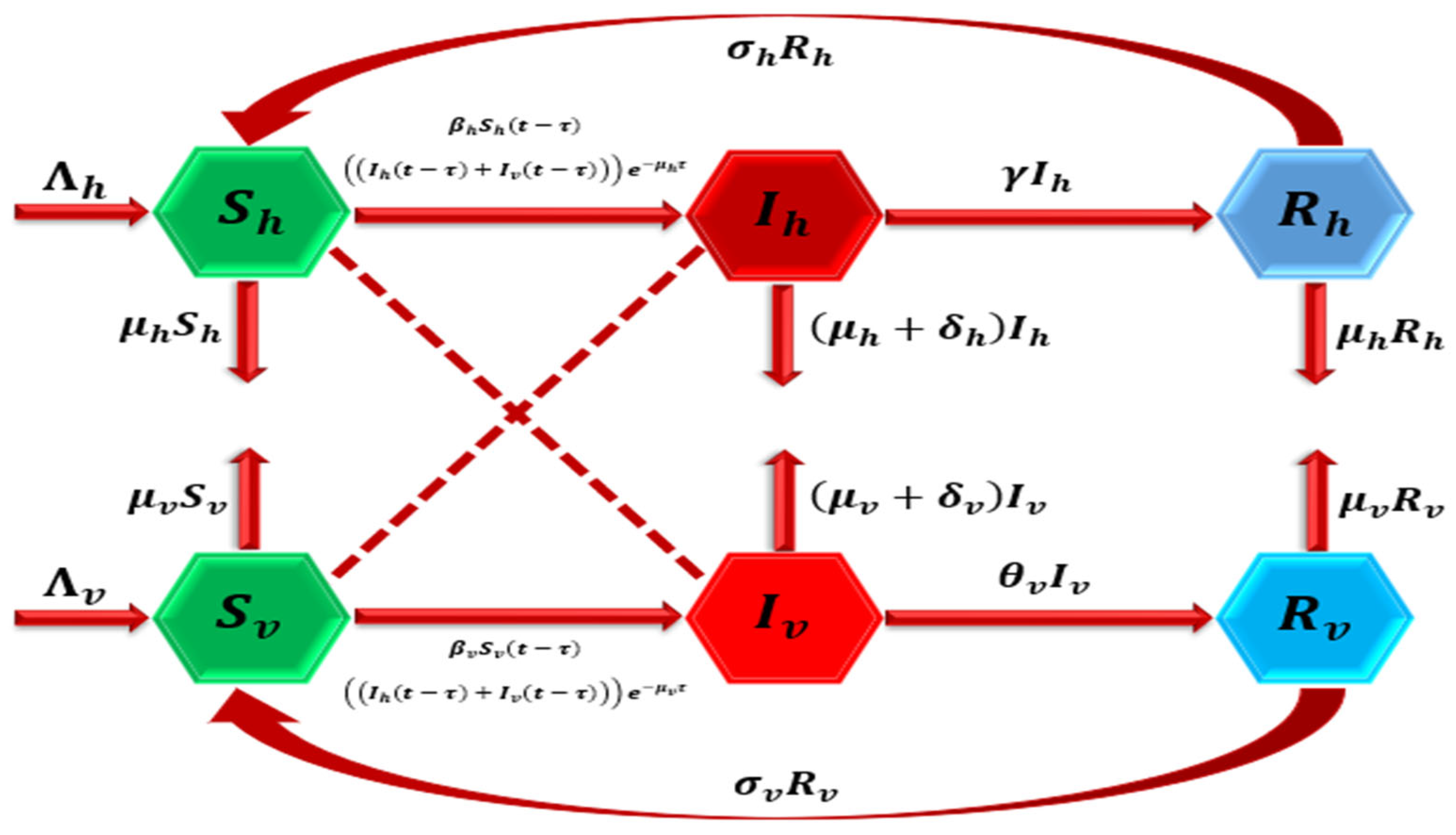
2. Model Formulation

Campylobacteriosis manifestations in people and animals are depicted in the model map in Figure 1. This illustration is important because it provides an understanding of the pattern of disease transmission in both people and animals. The whole human and animal populations constituted the two divides of our model. According to their condition inside the system, these populations are also split into six sub-compartments at any given moment. $\left(N_h\right)$, The whole human population is split into subpopulations: susceptible humans $\left(S_h\right)$, infected humans$\left(I_h\right)$, and recovered humans, $\left(R_h\right)$. At a rate of recruitment $\left({\Lambda }_h\right)$, susceptible individuals are drawn into the population through immigration. They develop Campylobacteriosis at a rate of ${\beta }_h\left(I_h+I_v\right)$ by consuming tainted food and water, as well as from direct contact with diseased humans and animals. Humans with the infection recover from Campylobacteriosis at a rate of $\left(\gamma \right)$. The mortality rate from Campylobacteriosis is represented by $\left({\delta }_h\right)$. At a rate of $\left({\sigma }_h\right)$, recovered people may lose their immunity and reintegrate into the vulnerable group. The natural mortality rate from Campylobacteriosis in all human compartments is $\left({\mu }_h\right)$. Immigration brings in susceptible animals $\left(S_v\right)$ at a rate $\left({\Lambda }_v\right)$. Animals can develop Campylobacteriosis at a rate of ${\beta }_v\left(I_h+I_v\right)$ by consuming contaminated food, water, or by coming into contact with affected animals. The natural mortality rate of susceptible and infected animals is $\left({\mu }_v\right)$. The mortality rate of Campylobacteriosis-infected animals is $\left({\delta }_v\right)$, but their recovery rate might range from $\left(\theta \right)$ to $\left({\delta }_v\right)$. Hence, the total human population is $N_h=S_h+I_h+R_h$. The whole animal population, $N_v$, is split into subpopulations: recovered animals that are recovered $\left(R_v\right)$, infectious animals $\left(I_v\right)$, and susceptible animals $\left(S_v\right)$. Hence, the total animal population is $N_v=S_v+I_v+R_v$.

The deterministic model [1] is a basic epidemiological model that is derived by replacing first-order time derivatives with Caputo fractional derivatives of order α. Regarding this adjustment, we think that it will improve the representation of the Campylobacteriosis viral infection diffusion. It uses Caputo fractional derivatives to minimize the presence of memory effects that describe how the system depends on prior states and carries information about past infections in long-term memory. With this modification, the model is now able to capture the dynamics of infection over time into account, owing to the nonlinearity. The addition of ‘noise’ terms takes care of stochastic elements that are naturally occurring and characteristic features of biological processes. All of these stochastic components are then incorporated into the model to capture and analyze the interactions of the disease transmission specifics in the realistic scale of real-life accounts due to the stochastic nature of biological systems.

$$\left.\begin{array}{c}{}_0{}^c{D}_t^{\alpha }\left[S_h\right]={\Lambda }_h^{\alpha }-{\beta }_h^{\alpha }{S}_h\left(t-\tau \right)\left(\left(I_h\left(t-\tau \right)+I_v\left(t-\tau \right)\right)\right)e^{-{\mu }_h^{\alpha }\tau }-{\mu }_h^{\alpha }{S}_h+{\sigma }_h^{\alpha }{R}_h+{\sigma }_1^{\alpha }{S}_{h}d\left(B\right)\\ {}_0{}^c{D}_t^{\alpha }\left[I_h\right]={\beta }_h^{\alpha }{S}_h\left(t-\tau \right)\left(\left(I_h\left(t-\tau \right)+I_v\left(t-\tau \right)\right)\right)e^{-{\mu }_h^{\alpha }\tau }-\left({\gamma }^{\alpha }+{\delta }_h^{\alpha }+{\mu }_h^{\alpha }\right)I_h+{\sigma }_2^{\alpha }{I}_{h}d\left(B\right)\\ \begin{array}{c}{}_0{}^c{D}_t^{\alpha }\left[R_h\right]={\gamma }^{\alpha }{I}_h-\left({\sigma }_h^{\alpha }+{\mu }_h^{\alpha }\right)R_h+{\sigma }_3^{\alpha }{R}_{h}d\left(B\right)\\ {}_0{}^c{D}_t^{\alpha }\left[S_v\right]={\Lambda }_v^{\alpha }-{\beta }_v^{\alpha }{S}_v\left(t-\tau \right)\left(\left(I_h\left(t-\tau \right)+I_v\left(t-\tau \right)\right)\right)e^{-{\mu }_v^{\alpha }\tau }-{\mu }_v^{\alpha }{S}_v+{\sigma }_v^{\alpha }{R}_v+{\sigma }_4^{\alpha }{S}_{v}d\left(B\right)\\ \begin{array}{c}{}_0{}^c{D}_t^{\alpha }\left[I_v\right]={\beta }_v^{\alpha }{S}_v\left(t-\tau \right)\left(\left(I_h\left(t-\tau \right)+I_v\left(t-\tau \right)\right)\right)e^{-{\mu }_v^{\alpha }\tau }-\left({\theta }_v^{\alpha }+{\delta }_v^{\alpha }+{\mu }_v^{\alpha }\right)I_v+{\sigma }_5^{\alpha }{I}_{v}d\left(B\right)\\ {}_0{}^c{D}_t^{\alpha }\left[R_v\right]={\theta }_v^{\alpha }{I}_v-\left({\sigma }_v^{\alpha }+{\mu }_v^{\alpha }\right)R_v+{\sigma }_6^{\alpha }{R}_{v}d\left(B\right)\end{array}\end{array}\end{array}\right\}$$

(1)

This approach describes the dispersion of random loads in a system or stochastic fluctuations characterized by the symbols: ${\sigma }_i^{\alpha };i=1, 2, 3, 4, 5, 6$. Let B(t) denote Brownian motion, which is a continuous stochastic process for $t\ge 0$. The parameter $\tau$ is used as a time delay in the system, so $\tau <t$, and thus the influence of delayed feedback is only visible after a certain period.

Preliminaries: In the conceptualization of Caputo, the following foundational preliminary definitions are crucial for a deep and thorough understanding of the fractional derivative concept:

Definition 1.

For a function $\mathcal{q}\in C_n$, the Caputo fractional derivative of order $\alpha \in (\mathcal{m}-1,\mathcal{m}),\mathcal{m}\in N$ is

$${}_0{}^c{D}_t^{\alpha }\mathcal{q}\left(t\right)={\displaystyle \frac{1}{\Gamma \left(\mathcal{m}-\alpha \right)}}{\int }_0^t{\displaystyle \frac{{\mathcal{q}}^{\mathcal{m}}\left(\mathfrak{T}\right)d\mathfrak{T}}{{\left(t-\mathfrak{T}\right)}^{\alpha +1-\mathcal{m}}}}$$

(2)

Definition 2.

For the function $\mathcal{q}\left(t\right)$, the expression describes the equivalent fractional integral with order $\alpha >0$.

$$I_t^{\alpha }\mathcal{q}\left(t\right)={\displaystyle \frac{1}{\Gamma \left(\alpha \right)}}{\int }_0^t{\left(t-\mathfrak{T}\right)}^{\alpha -1}\mathcal{q}\left(\mathfrak{T}\right)d\mathfrak{T}$$

(3)

where “$\Gamma$” is the gamma function displayed.

2.1. Existence and Uniqueness of the Stochastic Fractional Delayed Model

This section aims to prove the existence of solutions and their uniqueness for the stochastic fractional delayed model represented by model (1), which describes the Campylobacteriosis disease. To that end, we appeal to the notion of fractional integrals appropriate for this setting by reflecting on the initial conditions of a system to show these features. In this regard, the models adopt the assumption that ${\sigma }_i^{\alpha }=0; i=1, 2, 3, 4, 5, 6$ as there are no interacting deterministic components. This assumption offered the advantage of removing stochastic noise, and, thus, only the deterministic behaviors of the system can be observed. After that, using the necessary mathematical instruments involving the Caputo derivative, it is proved that the fractional delayed model of Campylobacteriosis has a unique solution.

$$\left.\begin{array}{c}{S}_h={S_h}_0+{\displaystyle \frac{1}{\Gamma \left(\alpha \right)}}{\int }_0^t{\left(t-s\right)}^{\alpha -1}{\mathcal{P}}_1\left(s,S_h\right)ds.\\ I_h={I_h}_0+{\displaystyle \frac{1}{\Gamma \left(\alpha \right)}}{\int }_0^t{\left(t-s\right)}^{\alpha -1}{\mathcal{P}}_2\left(s,I_h\right)ds.\\ \begin{array}{c}{R}_h={R_h}_0+{\displaystyle \frac{1}{\Gamma \left(\alpha \right)}}{\int }_0^t{\left(t-s\right)}^{\alpha -1}{\mathcal{P}}_3\left(s,R_h\right)ds.\\ S_v={S_v}_0+{\displaystyle \frac{1}{\Gamma \left(\alpha \right)}}{\int }_0^t{\left(t-s\right)}^{\alpha -1}{\mathcal{P}}_4\left(s,S_v\right)ds.\\ \begin{array}{c}{I}_v={I_v}_0+{\displaystyle \frac{1}{\Gamma \left(\alpha \right)}}{\int }_0^t{\left(t-s\right)}^{\alpha -1}{\mathcal{P}}_5\left(s,I_v\right)ds\\ R_v={R_v}_0+{\displaystyle \frac{1}{\Gamma \left(\alpha \right)}}{\int }_0^t{\left(t-s\right)}^{\alpha -1}{\mathcal{P}}_5\left(s,R_v\right)ds\end{array}\end{array}\end{array}\right\}$$

(4)

In system (4) the functions are defined under the integral are as follows:

$$\left.\begin{array}{c}{\mathcal{P}}_1\left(t,S_h\right)={\Lambda }_h^{\alpha }-{\beta }_h^{\alpha }{S}_h\left(I_h+I_v\right)e^{-{\mu }_h^{\alpha }\tau }-{\mu }_h^{\alpha }{S}_h+{\sigma }_h^{\alpha }{R}_h\\ {\mathcal{P}}_2\left(t,I_h\right)={\beta }_h^{\alpha }{S}_h\left(I_h+I_v\right)e^{-{\mu }_h^{\alpha }\tau }-\left({\gamma }^{\alpha }+{\delta }_h^{\alpha }+{\mu }_h^{\alpha }\right)I_h\\ \begin{array}{c}{\mathcal{P}}_3\left(t,R_h\right)={\gamma }^{\alpha }{I}_h-\left({\sigma }_h^{\alpha }+{\mu }_h^{\alpha }\right)R_h\\ {\mathcal{P}}_4\left(t,S_v\right)={\Lambda }_v^{\alpha }-{\beta }_v^{\alpha }{S}_v\left(I_h+I_v\right)e^{-{\mu }_v^{\alpha }\tau }-{\mu }_v^{\alpha }{S}_v+{\sigma }_v^{\alpha }{R}_v\\ \begin{array}{c}{\mathcal{P}}_5\left(t,I_v\right)={\beta }_v^{\alpha }{S}_v\left(I_h+I_v\right)e^{-{\mu }_v^{\alpha }\tau }-\left({\theta }_v^{\alpha }+{\delta }_v^{\alpha }+{\mu }_v^{\alpha }\right)I_v\\ {\mathcal{P}}_6\left(t,R_v\right)={\theta }_v^{\alpha }{I}_v-\left({\sigma }_v^{\alpha }+{\mu }_v^{\alpha }\right)R_v\end{array}\end{array}\end{array}\right\}$$

(5)

There is also a general assumption that the limiting functions $S_h,I_h,R_h,S_v,I_v,\mathrm{a}\mathrm{n}\mathrm{d}{R}_v$ are strictly non-negative. For these functions of asymptotic behavior to achieve, positive constants ${ℇ}_1,{ℇ}_2,{ℇ}_3,{ℇ}_4,{ℇ}_5,\mathrm{a}\mathrm{n}\mathrm{d}{ℇ}_6$ should be set. In such a manner, as the period (t) undergoes an increasing scale, the values of $S_h,I_h,R_h,S_v,I_v,\mathrm{a}\mathrm{n}\mathrm{d}{R}_v$ tend to approach particular positive values below which no greater number than a predetermined one can be found (those will be denoted by ${ℇ}_1,{ℇ}_2,{ℇ}_3,{ℇ}_4,{ℇ}_5,\mathrm{a}\mathrm{n}\mathrm{d}{ℇ}_6$).

Such that

$$‖S_h‖\le {ℇ}_1,‖I_h‖\le {ℇ}_2,‖R_h‖\le {ℇ}_3,‖S_v‖\le {ℇ}_4,‖I_v‖\le {ℇ}_5\mathrm{a}\mathrm{n}\mathrm{d}‖R_v‖\le {ℇ}_6.$$

Theorem 1.

Let ${\mathcal{P}}_i$be functions for $i=1, 2, 3, 4, 5, 6$with $0\le \mathcal{W}=max\{\mathrm{1,2},\mathrm{3,4},\mathrm{5,6}\}<1$. satisfying $0\le \mathcal{W}<1$, and assume ${\sigma }_i^{\alpha }=0; i=1, 2, 3, 4, 5, 6$. Then, each function ${\mathcal{F}}_i$satisfies the Lipschitz condition and is a contraction mapping.

Proof. 

First of all, we consider the function ${\mathcal{F}}_1$ as our main concern. To further understand the associations and consequences of the following functions, let us define and analyze them in this context: $S_h$ and $S_h^1$.

$$\left.\begin{array}{c}‖{\mathcal{F}}_1\left(t,S_h\right)-{\mathcal{F}}_2\left(t,S_h^1\right)‖=‖{\beta }_h^{\alpha }\left(S_h-S_h^1\right)\left(I_h+I_v\right)e^{-{\mu }_h^{\alpha }\tau }+{\mu }_h^{\alpha }\left(S_h-S_h^1\right)‖\\ ‖{\mathcal{F}}_1\left(t,S_h\right)-{\mathcal{F}}_2\left(t,S_h^1\right)‖\le ‖{\beta }_h^{\alpha }\left(S_h-S_h^1\right)\left(I_h+I_v\right)e^{-{\mu }_h^{\alpha }\tau }‖+‖{\mu }_h^{\alpha }\left(S_h-S_h^1\right)‖\\ \begin{array}{c}‖{\mathcal{F}}_1\left(t,S_h\right)-{\mathcal{F}}_2\left(t,S_h^1\right)‖\le \left({\beta }_h^{\alpha }{e}^{-{\mu }_h^{\alpha }\tau }‖\left(I_h+I_v\right)‖+{\mu }_h^{\alpha }\right)‖S_h-S_h^1‖\\ ‖{\mathcal{F}}_1\left(t,S_h\right)-{\mathcal{F}}_2\left(t,S_h^1\right)‖\le \left({\beta }_h^{\alpha }{e}^{-{\mu }_h^{\alpha }\tau }\left({ℇ}_2+{ℇ}_5\right)+{\mu }_h^{\alpha }\right)‖S_h-S_h^1‖\\ \begin{array}{c}‖{\mathcal{F}}_1\left(t,S_h\right)-{\mathcal{F}}_2\left(t,S_h^1\right)‖\le {\xi }_1‖S_h-S_h^1‖\end{array}\end{array}\end{array}\right\}$$

(6)

Consider this expression: ${\xi }_1=\left({\beta }_h^{\alpha }{e}^{-{\mu }_h^{\alpha }\tau }\left({ℇ}_2+{ℇ}_5\right)+{\mu }_h^{\alpha }\right)$. This equation indicates that the Lipschitz condition is satisfied, given ${\xi }_1$. To ensure that the Lipschitz criteria apply for the functions ${\mathcal{F}}_i$, where $i=2, 3, 4, 5, 6$, we may employ an analogous method that takes advantage of the nature of these functions. Additionally, the fact that these functions are contractions is confirmed under the specific conditions that $\mathcal{W}=max\{\mathrm{1,2},\mathrm{3,4},\mathrm{5,6}\}<1$ and $\mathcal{W}=max\{\mathrm{1,2},\mathrm{3,4},\mathrm{5,6}\}<1$. This implies the presence of contractile properties in the system, which are required for the solutions to stabilize and converge. It is also noteworthy that the system, as shown by system (6), has a consistent expression. For the overall validity and stability of the model to be maintained, the solutions must be continuous for them to behave smoothly over the designated domain.

$$\left.\begin{array}{c}{S_h}_n\left(t\right)={\displaystyle \frac{1}{\Gamma \left(\alpha \right)}}{\int }_0^t{\left(t-s\right)}^{\alpha -1}{\mathcal{F}}_1\left(s,{S_h}_{n-1}\right)ds.\\ {I_h}_n\left(t\right)={\displaystyle \frac{1}{\Gamma \left(\alpha \right)}}{\int }_0^t{\left(t-s\right)}^{\alpha -1}{\mathcal{F}}_2\left(s,{I_h}_{n-1}\right)ds\\ \begin{array}{c}{R_h}_n\left(t\right)={\displaystyle \frac{1}{\Gamma \left(\alpha \right)}}{\int }_0^t{\left(t-s\right)}^{\alpha -1}{\mathcal{F}}_3\left(s,{R_h}_{n-1}\right)ds\\ {S_v}_n\left(t\right)={\displaystyle \frac{1}{\Gamma \left(\alpha \right)}}{\int }_0^t{\left(t-s\right)}^{\alpha -1}{\mathcal{F}}_4\left(s,{S_v}_{n-1}\right)ds.\\ \begin{array}{c}{I_v}_n\left(t\right)={\displaystyle \frac{1}{\Gamma \left(\alpha \right)}}{\int }_0^t{\left(t-s\right)}^{\alpha -1}{\mathcal{F}}_5\left(s,{I_v}_{n-1}\right)ds.\\ {R_v}_n\left(t\right)={\displaystyle \frac{1}{\Gamma \left(\alpha \right)}}{\int }_0^t{\left(t-s\right)}^{\alpha -1}{\mathcal{F}}_6\left(s,{R_v}_{n-1}\right)ds\end{array}\end{array}\end{array}\right\}$$

(7)

The representation of the variation between the two terms in the system (7) is

$$\left.\begin{array}{c}{\psi }_{n-1}\left(t\right)=\left({S_h}_n\left(t\right)-{S_h}_{n-1}\left(t\right)\right)={\displaystyle \frac{1}{\Gamma \left(\alpha \right)}}{\int }_0^t\left({\mathcal{F}}_1\left(s,{S_h}_{n-1}\right)-{\mathcal{F}}_1\left(s,{S_h}_{n-2}\right)\right)ds.\\ {\phi }_{n-1}\left(t\right)=\left({I_h}_n\left(t\right)-{I_h}_{n-1}\left(t\right)\right)={\displaystyle \frac{1}{\Gamma \left(\alpha \right)}}{\int }_0^t\left({\mathcal{F}}_2\left(s,{I_h}_{n-1}\right)-{\mathcal{F}}_2\left(s,{I_h}_{n-2}\right)\right)ds\\ \begin{array}{c}{\vartheta }_{n-1}\left(t\right)=\left({R_h}_n\left(t\right)-{R_h}_{n-1}\left(t\right)\right)={\displaystyle \frac{1}{\Gamma \left(\alpha \right)}}{\int }_0^t\left({\mathcal{F}}_3\left(s,{R_h}_{n-1}\right)-{\mathcal{F}}_3\left(s,{R_h}_{n-2}\right)\right)ds.\\ {\varpi }_{n-1}\left(t\right)=\left({S_v}_n\left(t\right)-{S_v}_{n-1}\left(t\right)\right)={\displaystyle \frac{1}{\Gamma \left(\alpha \right)}}{\int }_0^t\left({\mathcal{F}}_4\left(s,{S_v}_{n-1}\right)-{\mathcal{F}}_4\left(s,{S_v}_{n-2}\right)\right)ds\\ \begin{array}{c}{\chi }_{n-1}\left(t\right)=\left({I_v}_n\left(t\right)-{I_v}_{n-1}\left(t\right)\right)={\displaystyle \frac{1}{\Gamma \left(\alpha \right)}}{\int }_0^t\left({\mathcal{F}}_5\left(s,{I_v}_{n-1}\right)-{\mathcal{F}}_5\left(s,{I_v}_{n-2}\right)\right)ds\\ {\Psi }_{n-1}\left(t\right)=\left({R_v}_n\left(t\right)-{R_v}_{n-1}\left(t\right)\right)={\displaystyle \frac{1}{\Gamma \left(\alpha \right)}}{\int }_0^t\left({\mathcal{F}}_6\left(s,{R_v}_{n-1}\right)-{\mathcal{F}}_6\left(s,{R_v}_{n-2}\right)\right)ds\end{array}\end{array}\end{array}\right\}$$

(8)

Therefore, we have

$$\begin{gathered} {S_h}_n\left(t\right)={\sum }_{i=0}^n{\psi }_i\left(t\right),{I_h}_n\left(t\right)={\sum }_{i=0}^n{\phi }_i\left(t\right),{R_h}_n\left(t\right)={\sum }_{i=0}^n{\vartheta }_i\left(t\right), \\ {S_v}_n\left(t\right)={\sum }_{i=0}^n{\varpi }_i\left(t\right),{I_v}_n\left(t\right)={\sum }_{i=0}^n{\chi }_i\left(t\right),{R_v}_n\left(t\right)={\sum }_{i=0}^n{\Psi }_i\left(t\right). \end{gathered}$$

(9)

Let,

$$\begin{gathered} ‖{\psi }_n\left(t\right)‖=‖{S_h}_n\left(t\right)-{S_h}_{n-1}\left(t\right)‖ \\ ‖{\psi }_n\left(t\right)‖={\displaystyle \frac{1}{\Gamma \left(\alpha \right)}}{\int }_0^t\left({\mathcal{F}}_1\left(s,{S_h}_{n-1}\right)-{\mathcal{F}}_1\left(s,{S_h}_{n-2}\right)\right)ds \\ ‖{\psi }_n\left(t\right)‖={\displaystyle \frac{{\xi }_1}{\Gamma \left(\alpha \right)}}{\int }_0^t‖{S_h}_n\left(t\right)-{S_h}_{n-1}\left(t\right)‖ds \\ ‖{\psi }_n\left(t\right)‖={\displaystyle \frac{{\xi }_1}{\Gamma \left(\alpha \right)}}{\int }_0^t{\psi }_{n-1}\left(t\right)ds \end{gathered}$$

(10)

When system (8)’s remaining equations are solved using the same approach, the following outcomes are obtained:

$$\begin{gathered} ‖{\phi }_n\left(t\right)‖={\displaystyle \frac{{\xi }_2}{\Gamma \left(\alpha \right)}}{\int }_0^t{\phi }_{n-1}\left(t\right)ds,‖{\vartheta }_n\left(t\right)‖={\displaystyle \frac{{\xi }_3}{\Gamma \left(\alpha \right)}}{\int }_0^t{\vartheta }_{n-1}\left(t\right)ds, \\ ‖{\varpi }_n\left(t\right)‖={\displaystyle \frac{{\xi }_4}{\Gamma \left(\alpha \right)}}{\int }_0^t{\varpi }_{n-1}\left(t\right)ds,‖{\chi }_n\left(t\right)‖={\displaystyle \frac{{\xi }_5}{\Gamma \left(\alpha \right)}}{\int }_0^t{\chi }_{n-1}\left(t\right)ds, \\ ‖{\Psi }_n\left(t\right)‖={\displaystyle \frac{{\xi }_6}{\Gamma \left(\alpha \right)}}{\int }_0^t{\Psi }_{n-1}\left(t\right)ds \end{gathered}$$

(11)

as required. □

Theorem 2.

Show $\left(i\right)$the existence of a uniform function defined in system (8). (ii) If there is a $t_{\ast }>1$ such that ${\displaystyle \frac{{\xi }_1}{\Gamma \left(\alpha \right)}}<1$. The model system has at least one solution if ${\displaystyle \frac{{\xi }_1}{\Gamma \left(\alpha \right)}}<1$ for $i=12, 3, 4, 5, 6$ and ${\sigma }_i^{\alpha }=0; i=1, 2, 3, 4, 5, 6$.

Proof. 

The functions $S_h,I_h,R_h,S_v,I_v,\mathrm{a}\mathrm{n}\mathrm{d}{R}_v$ are bounded, and each kernel ${\mathcal{P}}_i$ for $i=12, 3, 4, 5, 6$ fulfills the Lipschitz condition, leading to the derivation of the following relations:

$$\begin{gathered} ‖{\psi }_n\left(t\right)‖\le ‖S_h\left(0\right)‖{‖{\displaystyle \frac{{\xi }_1}{\Gamma \left(\alpha \right)}}\left(t\right)‖}^n,‖{\phi }_n\left(t\right)‖\le ‖I_h\left(0\right)‖{‖{\displaystyle \frac{{\xi }_2}{\Gamma \left(\alpha \right)}}\left(t\right)‖}^n, \\ ‖{\vartheta }_n\left(t\right)‖\le ‖R_h\left(0\right)‖{‖{\displaystyle \frac{{\xi }_3}{\Gamma \left(\alpha \right)}}\left(t\right)‖}^n,‖{\varpi }_n\left(t\right)‖\le ‖S_v\left(0\right)‖{‖{\displaystyle \frac{{\xi }_4}{\Gamma \left(\alpha \right)}}\left(t\right)‖}^n, \\ ‖{\chi }_n\left(t\right)‖\le ‖I_v\left(0\right)‖{‖{\displaystyle \frac{{\xi }_5}{\Gamma \left(\alpha \right)}}\left(t\right)‖}^n,‖{\Psi }_n\left(t\right)‖\le ‖R_v\left(0\right)‖{‖{\displaystyle \frac{{\xi }_6}{\Gamma \left(\alpha \right)}}\left(t\right)‖}^n. \end{gathered}$$

(12)

In the system (12) demonstration, the function given in (9) is demonstrated to exist and be uniform.

To prove (ii), one must show that the system of solutions of (1) is reached by $S_h,I_h,R_h,S_v,I_v,\mathrm{a}\mathrm{n}\mathrm{d}{R}_v$. Specifically, we define ${S_h}_n,{I_h}_n,{R_h}_n,{S_v}_n,{I_v}_n,\mathrm{a}\mathrm{n}\mathrm{d}{R_v}_n$ as terms that function after $n$ variations are performed, so that

$$\begin{gathered} S_h\left(t\right)-S_h\left(0\right)={S_h}_n\left(t\right)-M_n\left(t\right),I_h\left(t\right)-I_h\left(0\right)={I_h}_n\left(t\right)-N_n\left(t\right), \\ {R}_h\left(t\right)-R_h\left(0\right)={R_h}_n\left(t\right)-X_n\left(t\right),S_v\left(t\right)-S_v\left(0\right)={S_v}_n\left(t\right)-Y_n\left(t\right), \\ {I}_v\left(t\right)-I_v\left(0\right)={I_v}_n\left(t\right)-Z_n\left(t\right),R_v\left(t\right)-R_v\left(0\right)={R_v}_n\left(t\right)-O_n\left(t\right), \end{gathered}$$

(13)

Utilizing the triangle inequality in conjunction with ${\xi }_1$ Lipschitz condition, we conclude that

$$\begin{gathered} ‖M_n\left(t\right)‖={\displaystyle \frac{1}{\Gamma \left(\alpha \right)}}{\int }_0^t\left({\mathcal{F}}_1\left(s,{S_h}_{n-1}\right)-{\mathcal{F}}_1\left(s,{S_h}_{n-2}\right)\right)ds \\ ‖M_n\left(t\right)‖\le {\displaystyle \frac{{\xi }_1}{\Gamma \left(\alpha \right)}}‖{S_h}_n\left(t\right)-{S_h}_{n-1}\left(t\right)‖ \end{gathered}$$

(14)

Repetitively carrying out the procedure in (14), we obtain

$$‖M_n\left(t\right)‖\le {‖{\displaystyle \frac{{\xi }_1}{\Gamma \left(\alpha \right)}}\left(t\right)‖}^{n+1}{ℇ}_1$$

(15)

Next, at $t_{\ast }$, one acquires

$$‖M_n\left(t\right)‖\le {‖{\displaystyle \frac{{\xi }_1}{\Gamma \left(\alpha \right)}}\left(t_{\ast }\right)‖}^{n+1}{ℇ}_1$$

(16)

Assuming $n\to \infty$ as the limit.

$$\underset{n\to \infty }{\lim }‖M_n\left(t\right)‖\le \underset{n\to \infty }{\lim }{‖{\displaystyle \frac{{\xi }_1}{\Gamma \left(\alpha \right)}}\left(t_{\ast }\right)‖}^{n+1}{ℇ}_1$$

(17)

By applying the hypothesis ${\displaystyle \frac{{\xi }_1}{\Gamma \left(\alpha \right)}}\left(t_{\ast }\right)<1$, we obtain the following from (17) yield:

$$\underset{n\to \infty }{\lim }‖M_n\left(t\right)‖=0$$

(18)

By using the same process as for n→ ∞, we obtain

$$‖N_n\left(t\right)‖\to 0,‖X_n\left(t\right)‖\to 0,‖Y_n\left(t\right)‖\to 0,‖Z_n\left(t\right)‖\to 0,‖O_n\left(t\right)‖\to 0.$$

(19)

Therefore, there is certainly a single solution as desired. □

Theorem 3.

Prove that the system (1) is unique if $\left(1-{\displaystyle \frac{{\xi }_1}{\Gamma \left(\alpha \right)}}\left(t\right)\right)>0$ for the assumption ${\sigma }_i^{\alpha }=0; i=1, 2, 3, 4, 5, 6$.

Proof. 

Consider that another collection of solutions to (1) is represented by the sets ${S_h}_1, {I_h}_1, {R_h}_1, {S_v}_1, {I_v}_1, \mathrm{a}\mathrm{n}\mathrm{d} {R_v}_1$.

$$\begin{gathered} ‖S_h\left(t\right)-{S_h}_1\left(t\right)‖={\displaystyle \frac{1}{\Gamma \left(\alpha \right)}}{\int }_0^t\left({\mathcal{F}}_1\left(s,S_h\right)-{\mathcal{F}}_1\left(s,{S_h}_1\right)\right)ds \\ ‖S_h\left(t\right)-{S_h}_1\left(t\right)‖\le {\displaystyle \frac{{\xi }_1}{\Gamma \left(\alpha \right)}}‖S_h\left(t\right)-{S_h}_1\left(t\right)‖ \end{gathered}$$

(20)

If the terms in (20) are rearranged, one obtains

$$\left(1-{\displaystyle \frac{{\xi }_1}{\Gamma \left(\alpha \right)}}\left(t\right)\right)‖S_h\left(t\right)-{S_h}_1\left(t\right)‖\le 0$$

(21)

By applying the hypothesis $\left(1-{\displaystyle \frac{{\xi }_1}{\Gamma \left(\alpha \right)}}\left(t\right)\right)>0$, we obtain the following from (21) yield:

$$‖S_h\left(t\right)-{S_h}_1\left(t\right)‖=0$$

(22)

It follows from this because $S_h\left(t\right)={S_h}_1\left(t\right)$. Applying the identical process to every solution for $i=2, 3, 4, 5, 6$ we arrive at the following:

$$\begin{gathered} S_h\left(t\right)={S_h}_1\left(t\right),I_h\left(t\right)={I_h}_1\left(t\right),R_h\left(t\right)={R_h}_1\left(t\right), \\ {S}_v\left(t\right)={S_v}_1\left(t\right),I_v\left(t\right)={I_v}_1\left(t\right),R_v\left(t\right)={R_v}_1\left(t\right) \end{gathered}$$

(23)

Hence, the theorem is proved. □

Theorem 4.

The solution of the given stochastic fractional delayed model (1) will be positive in ${\mathbb{R}}^{+6}$ according to its initial conditions for ${\sigma }_i^{\alpha }=0; i=1, 2, 3, 4, 5, 6.$

Proof. 

Whenever states are bounded by initial conditions, they have to be non-negative throughout the system. This means that any variable or parameter of this system cannot have a negative value at any stage within the presented framework of evolution. Non-negativity is important for convolutions because non-negative states are more physically realistic most of the time, while the negative states are undefined in most of the physical models. Consequently, we obtain the following:

$$\begin{gathered} {\left.{}_0{}^c{D}_t^{\alpha }\left[S_h\right]\right|}_{S_h=0}={\Lambda }^{\alpha }+{\sigma }_h^{\alpha }{R}_h\ge 0, {\left.{}_0{}^c{D}_t^{\alpha }\left[I_h\right]\right|}_{I_h=0}={\beta }_h^{\alpha }{S}_h\left(I_h+I_v\right)e^{-{\mu }_h^{\alpha }\tau }\ge 0, {\left.{}_0{}^c{D}_t^{\alpha }\left[R_h\right]\right|}_{R_h=0}={\gamma }^{\alpha }{I}_h\ge 0, \\ {\left.{}_0{}^c{D}_t^{\alpha }\left[S_v\right]\right|}_{S_v=0}={\Lambda }_v^{\alpha }+{\sigma }_v^{\alpha }{R}_v\ge 0,{\left.{}_0{}^c{D}_t^{\alpha }\left[I_v\right]\right|}_{I_v=0}={\beta }_v^{\alpha }{S}_v{I}_h{e}^{-{\mu }_v^{\alpha }\tau }\ge 0.{\left.{}_0{}^c{D}_t^{\alpha }\left[R_v\right]\right|}_{R_v=0}={\theta }_v^{\alpha }{I}_v\ge 0. \end{gathered}$$

It is worth emphasizing that a positive solution for the given stochastic fractional delayed model, as explained in system (1), is possible when the initial condition is inside the feasible area. This suggests that, despite the stochastic noise and or fractional values of time, the system remains manageable and will act within physically or biologically plausible restrictions and thus end up being positive. Thus, model stability and correspondence of the dynamics of the disease behavior remain unchanged if the initial values are located in the permissible area. □

Theorem 5.

For any time $t$ the system (1) in feasible region $\mathcal{G}=\left\{\left(S_h,I_h,R_h,S_v,I_v{R}_v\right)\in {\mathbb{R}}^{+6};0<N_h\left(t\right)\le {\displaystyle \frac{{\Lambda }_h^{\alpha }}{{\mu }_h^{\alpha }}},0<N_v\left(t\right)\le {\displaystyle \frac{{\Lambda }_v^{\alpha }}{{\mu }_v^{\alpha }}},\forall t\ge 0,\tau <t\right\}$, (where $N_h=S_h+I_h+R_h$ is total human population and $N_v=S_v+I_v+R_v$ is the animal total population) with initial condition is bounded with assumption ${\sigma }_i^{\alpha }=0; i=1, 2, 3, 4, 5, 6$

Proof. 

The total sum of human populations can be written as follows:

$$N_h\left(t\right)=S_h\left(t\right)+I_h\left(t\right)+R_h\left(t\right).$$

$${}_0{}^c{D}_t^{\alpha }{N}_h\left(t\right)={}_0{}^c{D}_t^{\alpha }{S}_h\left(t\right)+{}_0{}^c{D}_t^{\alpha }{I}_h\left(t\right)+{}_0{}^c{D}_t^{\alpha }{R}_h\left(t\right).$$

$${}_0{}^c{D}_t^{\alpha }{N}_h\left(t\right)={\Lambda }_h^{\alpha }-{\mu }_h^{\alpha }{N}_h\left(t\right).$$

$${}_0{}^c{D}_t^{\alpha }{N}_h\left(t\right)+{\mu }_h^{\alpha }{N}_h\left(t\right)={\Lambda }_h^{\alpha }.$$

Using the Laplace Transformation, we obtain

$$\mathcal{L}\left\{{}_0{}^c{D}_t^{\alpha }{N}_h\left(t\right)\right\}+\mathcal{L}\left\{{\mu }_h^{\alpha }{N}_h\right(t\left)\right\}={\Lambda }_h^{\alpha }\mathcal{L}\left\{1\right\}.$$

$$s^{\alpha }\mathcal{L}\{N_h(t)\}-s^{\alpha -1}{N}_h\left(0\right)+{\mu }_h^{\alpha }\mathcal{L}\left\{N_h\left(t\right)\right\}={\displaystyle \frac{{\Lambda }_h^{\alpha }}{s}}.$$

$$\left(s^{\alpha }+{\mu }_h^{\alpha }\right)\mathcal{L}\left\{N_h\left(t\right)\right\}=s^{\alpha -1}{N}_h\left(0\right)+{\displaystyle \frac{{\Lambda }_h^{\alpha }}{s}}.$$

$$\mathcal{L}\left\{N_h\left(t\right)\right\}={\displaystyle \frac{s^{\alpha -1}{N}_h\left(0\right)}{\left(s^{\alpha }+{\mu }_h^{\alpha }\right)}}+{\displaystyle \frac{{\Lambda }_h^{\alpha }}{s\left(s^{\alpha }+{\mu }_h^{\alpha }\right)}}.$$

By applying the Laplace inverse, we obtain

$$N_h\left(t\right)={\mathcal{L}}^{-1}\left\{{\displaystyle \frac{s^{\alpha -1}{N}_h\left(0\right)}{\left(s^{\alpha }+{\mu }_h^{\alpha }\right)}}+{\displaystyle \frac{{\Lambda }_h^{\alpha }}{s\left(s^{\alpha }+{\mu }_h^{\alpha }\right)}}\right\}.$$

$$N_h\left(t\right)=N_h\left(0\right)t^{1-1}{B}_{\alpha ,1}\left(-{\mu }_h^{\alpha }{t}^{\alpha }\right)+{\Lambda }_h^{\alpha }{t}^{\alpha }{B}_{\alpha ,1+\alpha }\left(-{\mu }_h^{\alpha }{t}^{\alpha }\right).$$

$$N_h(t)=N_h(0)B_{\alpha ,1}\left(-{\mu }_h^{\alpha }{t}^{\alpha }\right)+{\mu }_h^{\alpha }{\displaystyle \frac{{\Lambda }_h^{\alpha }}{{\mu }_h^{\alpha }}}{t}^{\alpha }{B}_{\alpha ,1+\alpha }\left(-{\mu }_h^{\alpha }{t}^{\alpha }\right).$$

Let $M=max\{N_h(0),{\displaystyle \frac{{\Lambda }_h^{\alpha }}{{\mu }_h^{\alpha }}}\}$.

$$N_h\left(t\right)\le M{B}_{\alpha ,1}\left(-{\mu }_h^{\alpha }{t}^{\alpha }\right)+M{\mu }_h^{\alpha }{t}^{\alpha }{B}_{\alpha ,1+\alpha }\left(-{\mu }_h^{\alpha }{t}^{\alpha }\right).$$

$$N_h\left(t\right)\le M[B_{\alpha ,1}\left(-{\mu }_h^{\alpha }{t}^{\alpha }\right)+{\mu }_h^{\alpha }{t}^{\alpha }{B}_{\alpha ,1+\alpha }\left(-{\mu }_h^{\alpha }{t}^{\alpha }\right)].$$

As, $E_{b,\beta }=z{E}_{b,b+\beta }\left(z\right)+{\displaystyle \frac{1}{\Gamma \left(\beta \right)}}$.

$$N_h(t)\le M[-{\mu }_h^{\alpha }{t}^{\alpha }{B}_{\alpha ,1+\alpha }\left(-{\mu }_h^{\alpha }{t}^{\alpha }\right)+{\displaystyle \frac{1}{\Gamma \left(1\right)}}+{\mu }_h^{\alpha }{t}^{\alpha }{B}_{\alpha ,1+\alpha }\left(-{\mu }_h^{\alpha }{t}^{\alpha }\right)].$$

$$N_h\left(t\right)\le M \mathrm{a}\mathrm{s} \Gamma \left(1\right)=1.$$

$$N_h\left(t\right)\le M.$$

Similarly, applying the same approach, the system is bounded and lies in the feasible region for the animal population. Therefore, the epidemiologically feasible region for the propagation of Campylobacteriosis is provided.

$$\mathcal{G}=\left\{\left(S_h,I_h,R_h,S_v,I_v{R}_v\right)\in {\mathbb{R}}^{+6};0<N_h\left(t\right)\le {\displaystyle \frac{{\Lambda }_h^{\alpha }}{{\mu }_h^{\alpha }}},0<N_v\left(t\right)\le {\displaystyle \frac{{\Lambda }_v^{\alpha }}{{\mu }_v^{\alpha }}},\forall t\ge 0,\tau <t\right\}$$

(24)

It is necessary and appropriate to use the stochastic fractional delayed model when studying and forecasting the characteristics of Campylobacteriosis from an epidemiological point of view. This model is appropriate and steady for using and comparing the introduction of disease in a given populace useful input into quantity relating to the Campylobacteriosis circulation parameters. Based on the developed equation, this positive and stable value informs about the invariance of the structure of the applied model to the Campylobacteriosis-related parameters. □

2.2. Model Equilibria and Reproduction Number

This section is devoted to the extraordinarily detailed compartments of the stochastic fractional delayed Campylobacteriosis model (1), namely in the disease dynamics section. It provides enhanced information about the system’s behavior under different scenarios, how the disease present equilibrium exists and has Campylobacteriosis stay in the population, whereas the disease-free equilibrium means the absence of the disease. It also tries to figure out how the disease can spread within the population stochastically.

Therefore,

Disease-Free Equilibrium:

$$DFE={\mathcal{O}}^0=\left({\left(S_h\right)}_0,{\left(I_h\right)}_0,{\left(R_h\right)}_0,{\left(S_v\right)}_0,{\left(I_v\right)}_0,{\left(R_v\right)}_0\right)=\left(\begin{array}{c}{\displaystyle \frac{{\Lambda }_h^{\alpha }}{{\mu }_h^{\alpha }}},\mathrm{0,0},{\displaystyle \frac{{\Lambda }_v^{\alpha }}{{\mu }_v^{\alpha }}},\mathrm{0,0}\end{array}\right).$$

(25)

Disease Present Equilibrium:

$$DPE={\mathcal{O}}^{\ast }=\left(S_h^{\ast },I_h^{\ast },R_h^{\ast },S_v^{\ast },I_v^{\ast },R_v^{\ast }\right).$$

(26)

$$S_h^{\ast }={\displaystyle \frac{\left({\gamma }^{\alpha }+{\delta }_h^{\alpha }+{\mu }_h^{\alpha }\right)I_h^{\ast }}{{\beta }_h^{\alpha }\left(I_h^{\ast }+I_v^{\ast }\right)e^{-{\mu }_h^{\alpha }\tau }}},I_h^{\ast }={\displaystyle \frac{\left({\theta }_v^{\alpha }+{\delta }_v^{\alpha }+{\mu }_v^{\alpha }\right)\left({\sigma }_v^{\alpha }+{\mu }_v^{\alpha }\right)\left({\mu }_v^{\alpha }+I_v^{\ast }\right)-\left({\sigma }_v^{\alpha }{\theta }_v^{\alpha }{I}_v^{\ast }\right){\beta }_v^{\alpha }{I}_v^{\ast }{e}^{-{\mu }_v^{\alpha }\tau }-{\Lambda }_v^{\alpha }\left({\sigma }_v^{\alpha }+{\mu }_v^{\alpha }{\beta }_v^{\alpha }{I}_v^{\ast }{e}^{-{\mu }_v^{\alpha }\tau }\right)}{{\Lambda }_v^{\alpha }\left({\sigma }_v^{\alpha }+{\mu }_v^{\alpha }\right){\beta }_v^{\alpha }{e}^{-{\mu }_v^{\alpha }\tau }+\left({\sigma }_v^{\alpha }{\theta }_v^{\alpha }\right){\beta }_v^{\alpha }{I}_v^{\ast }{e}^{-{\mu }_v^{\alpha }\tau }}},$$

$$R_h^{\ast }={\displaystyle \frac{{\gamma }^{\alpha }{I}_h^{\ast }}{\left({\sigma }_h^{\alpha }+{\mu }_h^{\alpha }\right)}}.S_v^{\ast }={\displaystyle \frac{\left({\theta }_v^{\alpha }+{\delta }_v^{\alpha }+{\mu }_v^{\alpha }\right)I_v^{\ast }}{{\beta }_v^{\alpha }\left(I_h^{\ast }+I_v^{\ast }\right)e^{-{\mu }_v^{\alpha }\tau }}}.R_v^{\ast }={\displaystyle \frac{{\theta }_v^{\alpha }{I}_v^{\ast }}{\left({\sigma }_v^{\alpha }+{\mu }_v^{\alpha }\right)}}.$$

$$I_v^{\ast }={\displaystyle \frac{\left({\gamma }^{\alpha }+{\delta }_h^{\alpha }+{\mu }_h^{\alpha }\right)\left({\sigma }_h^{\alpha }+{\mu }_h^{\alpha }\right){\beta }_h^{\alpha }{e}^{-{\mu }_h^{\alpha }\tau }-{\mu }_h^{\alpha }\left({\gamma }^{\alpha }+{\delta }_h^{\alpha }+{\mu }_h^{\alpha }\right)\left({\sigma }_h^{\alpha }+{\mu }_h^{\alpha }\right)+{\gamma }^{\alpha }{\beta }_h^{\alpha }{I}_h^{\ast }{e}^{-{\mu }_h^{\alpha }\tau }-{\Lambda }_h^{\alpha }\left({\sigma }_h^{\alpha }+{\mu }_h^{\alpha }\right){\beta }_h^{\alpha }{e}^{-{\mu }_h^{\alpha }\tau }}{{\Lambda }_h^{\alpha }\left({\sigma }_h^{\alpha }+{\mu }_h^{\alpha }\right){\beta }_h^{\alpha }{e}^{-{\mu }_h^{\alpha }\tau }-{\beta }_h^{\alpha }{e}^{-{\mu }_h^{\alpha }\tau }\left({\gamma }^{\alpha }+{\delta }_h^{\alpha }+{\mu }_h^{\alpha }\right)-{\gamma }^{\alpha }{\beta }_h^{\alpha }{I}_h^{\ast }{e}^{-{\mu }_h^{\alpha }\tau }}}.$$

For an infectious disease, the reproduction number indicates whether the disease is likely to be prevalent and controlled or receding and eliminated in a population. If the reproduction number is less than one, the disease may be manageable; if the reproduction number is greater than one, the disease is expected to continue spreading. The next-generation matrix approach is used to calculate the basic reproduction number.

$$R_0={\displaystyle \frac{{\Lambda }_h^{\alpha }{\beta }_h^{\alpha }{e}^{-{\mu }_h^{\alpha }\tau }}{{\mu }_h^{\alpha }\left({\gamma }^{\alpha }+{\delta }_h^{\alpha }+{\mu }_h^{\alpha }\right)}}.$$

(27)

Theorem 6.

Disease-free equilibrium (25) is locally asymptotically stable for $\alpha \in (0,1)$ if $R_0<1$ with the assumption of ${\sigma }_i^{\alpha }=0; i=1, 2, 3, 4, 5, 6$.

Proof. 

The stochastic fractional delayed model (1) is linearized around (25) to obtain a $6\times 6$ dimensional Jacobian matrix with negative real components and eigenvalues,

$${\lambda }_1=-{\mu }_h^{\alpha },{\lambda }_2=-\left({\sigma }_h^{\alpha }+{\mu }_h^{\alpha }\right).{\lambda }_3=-{\mu }_v^{\alpha }, {\lambda }_4=-\left({\sigma }_v^{\alpha }+{\mu }_v^{\alpha }\right),$$

The second-degree polynomial follows as

$$A_2{\lambda }^2+A_1\lambda +A_0=0.$$

Here,

$$\begin{gathered} A_2=1. \\ {A}_1=a_1-a_2+a_3-a_4, \\ {A}_0=\left(a_1-a_2\right)\left(a_3-a_4\right)-a_1{a}_3. \\ {a}_1={\beta }_h^{\alpha }{S}_h{e}^{-{\mu }_h^{\alpha }\tau }, a_2=\left({\gamma }^{\alpha }+{\delta }_h^{\alpha }+{\mu }_h^{\alpha }\right), a_3={\beta }_v^{\alpha }{S}_v{e}^{-{\mu }_v^{\alpha }\tau }, a_4=\left({\theta }_v^{\alpha }+{\delta }_v^{\alpha }+{\mu }_v^{\alpha }\right). \end{gathered}$$

Since all four eigenvalues are negative, the disease-free equilibrium point is locally asymptotically stable. According to the Routh–Hurwitz criterion for a second-order polynomial, local stability is ensured when all coefficients $A_2$, $A_1,$and $A_0$ are positive. This condition holds when $R_0<1$. Therefore, the disease-free equilibrium of the stochastic fractional delayed model (1) is locally stable if $R_0<1.$ Conversely, if $R_0>1$, the equilibrium becomes unstable. □

Theorem 7.

The stochastic fractional delayed model (1) is globally asymptotical stable (GAS) at disease-free equilibrium, ${\mathcal{O}}^0$, if $R_0<1$ with the assumption of ${\sigma }_i^{\alpha }=0; i=1, 2, 3, 4, 5, 6$.

Proof. 

The Volterra Lyapunov function $\mathcal{L}:\mathcal{G}\to \mathbb{R}$ is defined as

$$\mathcal{L}\left(t\right)=\left[S_h-{\left(S_h\right)}_0-{\left(S_h\right)}_{0}log{\displaystyle \frac{S_h}{{\left(S_h\right)}_0}}\right]+I_h+R_h+\left[S_v-{\left(S_v\right)}_0-{\left(S_v\right)}_{0}log{\displaystyle \frac{S_v}{{\left(S_v\right)}_0}}\right]+I_v+R_v.$$

$${}_0{}^c{D}_t^{\alpha }\mathcal{L}\left(t\right)=\left[{\displaystyle \frac{S_h-{\left(S_h\right)}_0}{S_h}}\right]D_t^{\alpha }{S}_h+D_t^{\alpha }{I}_h+D_t^{\alpha }{R}_h+\left[{\displaystyle \frac{S_v-{\left(S_v\right)}_0}{S_v}}\right]D_t^{\alpha }{S}_v+D_t^{\alpha }{I}_v+D_t^{\alpha }{R}_v.$$

$$\begin{gathered} {}_0{}^c{D}_t^{\alpha }\mathcal{L}\left(t\right)=\left[{\displaystyle \frac{S_h-{\left(S_h\right)}_0}{S_h}}\right]\left({\Lambda }_h^{\alpha }-{\beta }_h^{\alpha }{S}_h\left(I_h+I_v\right)e^{-{\mu }_h^{\alpha }\tau }-{\mu }_h^{\alpha }{S}_h+{\sigma }_h^{\alpha }{R}_h\right)+\left({\beta }_h^{\alpha }{S}_h\left(I_h+I_v\right)e^{-{\mu }_h^{\alpha }\tau }- \\ \left({\gamma }^{\alpha }+{\delta }_h^{\alpha }+{\mu }_h^{\alpha }\right)I_h\right)+\left({\gamma }^{\alpha }{I}_h-\left({\sigma }_h^{\alpha }+{\mu }_h^{\alpha }\right)R_h\right)+\left[{\displaystyle \frac{S_v-{\left(S_v\right)}_0}{S_v}}\right]\left({\Lambda }_v^{\alpha }-{\beta }_v^{\alpha }{S}_v\left(I_h+I_v\right)e^{-{\mu }_v^{\alpha }\tau }-{\mu }_v^{\alpha }{S}_v+{\sigma }_v^{\alpha }{R}_v\right)+ \\ \left({\beta }_v^{\alpha }{S}_v\left(I_h+I_v\right)e^{-{\mu }_v^{\alpha }\tau }-\left({\theta }_v^{\alpha }+{\delta }_v^{\alpha }+{\mu }_v^{\alpha }\right)I_v\right)+\left({\theta }_v^{\alpha }{I}_v-\left({\sigma }_v^{\alpha }+{\mu }_v^{\alpha }\right)R_v\right). \end{gathered}$$

$$\begin{gathered} {}_0{}^c{D}_t^{\alpha }\mathcal{L}\left(t\right)\le -\left({\Lambda }_h^{\alpha }+{\sigma }_h^{\alpha }{R}_h\right){\displaystyle \frac{{\left(S_h-{\left(S_h\right)}_0\right)}^2}{S_h{S}_h^0}}-\left({\delta }_h^{\alpha }+{\mu }_h^{\alpha }\right)I_h\left(1-{\displaystyle \frac{{\beta }_h^{\alpha }{S}_h{e}^{-{\mu }_h^{\alpha }\tau }}{\left({\delta }_h^{\alpha }+{\mu }_h^{\alpha }\right)}}\right)-\left({\sigma }_h^{\alpha }+{\mu }_h^{\alpha }\right)R_h-\left({\Lambda }_v^{\alpha }+ \\ {\sigma }_v^{\alpha }{R}_v\right){\displaystyle \frac{{\left(S_v-{\left(S_v\right)}_0\right)}^2}{S_v{S}_v^0}}-\left({\delta }_v^{\alpha }+{\mu }_v^{\alpha }\right)I_v\left[1-{\displaystyle \frac{{\beta }_v^{\alpha }{S}_v{e}^{-{\mu }_v^{\alpha }\tau }}{\left({\delta }_v^{\alpha }+{\mu }_v^{\alpha }\right)}}\right]-\left({\sigma }_v^{\alpha }+{\mu }_v^{\alpha }\right)R_v. \end{gathered}$$

This implies that ${}_0{}^c{D}_t^{\alpha }\mathcal{L}\le 0$ if $R_0<1$, and ${}_0{}^c{D}_t^{\alpha }\mathcal{L}=0$ if $S_h={\left(S_h\right)}_0, S_v={\left(S_v\right)}_0, I_h=R_h=I_v=R_v=0$. Therefore, ${\mathcal{O}}^0$ is globally asymptotically stable. □

Theorem 8.

Disease-present equilibrium (26) is locally asymptotically stable for $\alpha \in (0,1)$ if $R_0>1$ with the assumption of ${\sigma }_i^{\alpha }=0; i=1, 2, 3, 4, 5, 6$.

Proof. 

The stochastic fractional delayed model (1) is linearized around (26) to obtain a $6\times 6$ dimensional Jacobian matrix with negative real components and eigenvalues;

The 6th degree polynomial follows as

$$A_6{\lambda }^6+A_5{\lambda }^5+A_4{\lambda }^4+A_3{\lambda }^3+A_2{\lambda }^2+A_1\lambda +A_0=0.$$

Here,

$$A_6=1.$$

$$A_5=a_1+a_8+a_{11}-a_{10}+a_6-a_5.$$

$$A_4=\left(1+a_1\right)\left(a_8{a}_{11}-a_8{a}_{10}-a_{10}{a}_{11}+a_9{a}_7+\left(a_6-a_5\right)\left(a_8+a_{11}-a_{10}\right)-a_3{a}_6+a_3{a}_7\right).$$

$$\begin{gathered} A_3=\left(1+a_1\right)\left(a_7{a}_9{a}_{11}-a_8{a}_9{a}_{11}-a_9{\theta }_v^{\alpha }{\sigma }_v^{\alpha }+\left(a_6-a_5\right)\left(a_7{a}_9{a}_{11}-a_8{a}_9{a}_{11}-a_9{\theta }_v^{\alpha }{\sigma }_v^{\alpha }\right)- \\ {a}_3{a}_6\left(a_8+a_{11}-a_{10}\right)+a_3{a}_6{a}_7\right)+a_3{a}_7{a}_9+a_3{a}_7{a}_4-a_4{\sigma }_h^{\alpha }{\gamma }^{\alpha }. \end{gathered}$$

$$\begin{gathered} A_2=\left(1+a_1\right)\left(\left(a_6-a_5\right)\left(a_7{a}_9{a}_{11}-a_8{a}_9{a}_{11}-a_9{\theta }_v^{\alpha }{\sigma }_v^{\alpha }\right)-a_3{a}_6\left(a_8+a_{11}-a_{10}\right)+a_7{a}_9- \\ {a}_7{a}_3\left(a_6{a}_9-a_6{a}_8-a_6{a}_{11}+a_{11}{a}_9-a_8{a}_{11}\right)\right)-a_8{a}_4{\sigma }_h^{\alpha }{\gamma }^{\alpha }-\left(a_{10}-a_{11}\right)a_4{\sigma }_h^{\alpha }{\gamma }^{\alpha }+a_4{a}_3\left(a_6-a_{11}\right)+ \\ {a}_4{a}_3{a}_7\left(a_8-a_9\right). \end{gathered}$$

$$\begin{gathered} A_1=\left(1+a_1\right)\left(a_2{a}_6-a_8{a}_4\left(a_{10}-a_{11}\right){\sigma }_h^{\alpha }{\gamma }^{\alpha }+a_4{a}_7{a}_9{a}_{11}{\sigma }_h^{\alpha }{\gamma }^{\alpha }+a_4{a}_7{a}_9{\sigma }_h^{\alpha }{\gamma }^{\alpha }+a_4{a}_3{a}_6{a}_{11}{a}_{11}+ \\ {a}_3{a}_4{a}_7\left(a_8-a_9\right)\left(a_6-a_{11}\right)+a_3{a}_6(a_8{a}_9{a}_{11}+a_9{\theta }_v^{\alpha }{\sigma }_v^{\alpha }-a_7{a}_9{a}_{11})\right). \end{gathered}$$

$$\begin{gathered} A_0=\left(1+a_1\right)\left(a_3{a}_6{a}_7{a}_{11}\left(a_8-a_9\right)\right)-a_4{a}_8{a}_{10}{a}_{11}{\sigma }_h^{\alpha }{\gamma }^{\alpha }+a_2{a}_4{a}_6-a_4{a}_{10}{a}_{11}{\sigma }_h^{\alpha }{\gamma }^{\alpha }-\left(a_4{\sigma }_h^{\alpha }{\gamma }^{\alpha }\right)\left(a_9{\sigma }_h^{\alpha }{\sigma }_v^{\alpha }\right)+ \\ {a}_3{a}_4{a}_6{a}_{11}{a}_7\left(a_8-a_9\right). \end{gathered}$$

Also,

$$a_1={\beta }_h^{\alpha }\left(I_h^{\ast }+I_v^{\ast }\right)e^{-{\mu }_h^{\alpha }\tau }+{\mu }_h^{\alpha },a_2={\beta }_h^{\alpha }{S}_h^{\ast }{e}^{-{\mu }_h^{\alpha }\tau },a_3={\beta }_h^{\alpha }{S}_h^{\ast }{e}^{-{\mu }_h^{\alpha }\tau },a_4={\beta }_h^{\alpha }\left(I_h^{\ast }+I_v^{\ast }\right)e^{-{\mu }_h^{\alpha }\tau },$$

$$\begin{gathered} a_5={\beta }_h^{\alpha }{S}_h^{\ast }{e}^{-{\mu }_h^{\alpha }\tau }-\left({\gamma }^{\alpha }+{\delta }_h^{\alpha }+{\mu }_h^{\alpha }\right), a_6=\left({\sigma }_h^{\alpha }+{\mu }_h^{\alpha }\right), a_7={\beta }_v^{\alpha }{S}_v^{\ast }{e}^{-{\mu }_v^{\alpha }\tau }. a_8={\beta }_v^{\alpha }\left(I_h^{\ast }+I_v^{\ast }\right)e^{-{\mu }_v^{\alpha }\tau }+{\mu }_v^{\alpha },.a_9= \\ {\beta }_v^{\alpha }\left(I_h^{\ast }+I_v^{\ast }\right)e^{-{\mu }_v^{\alpha }\tau },a_{10}={\beta }_v^{\alpha }{S}_v^{\ast }{e}^{-{\mu }_v^{\alpha }\tau }-\left({\theta }_v^{\alpha }+{\delta }_v^{\alpha }+{\mu }_v^{\alpha }\right),a_{11}=\left({\sigma }_v^{\alpha }+{\mu }_v^{\alpha }\right). \end{gathered}$$

Which is the 6th-degree polynomial where the coefficients of the polynomial are positive with $A_1{A}_4-A_2{A}_3>0, A_1{A}_6-{\left(A_3\right)}^2>0, A_1{A}_6{A}_4-A_2{A}_5{A}_3+{\left(A_2\right)}^2{A}_6-{\left(A_5\right)}^2>0$. So, using the Routh–Hurwitz criterion for a 6th-degree polynomial, the coefficient of the characteristic equation is positive with the constraint $R_0>1.$ Hence, the disease-present equilibrium of the given system (1) is stable in the sense of being locally stable. Else, if $R_0<1,$ then Routh–Hurwitz’s condition for stability is violated. Thus, (29) is unstable in the sense of local sense. □

Theorem 9.

The stochastic fractional delayed model (1) is globally asymptotical stable (GAS) at disease present equilibrium, (${\mathcal{O}}^{\ast }$) if$R_0>1$ with the assumption of ${\sigma }_i^{\alpha }=0; i=1, 2, 3, 4, 5, 6$.

Proof. 

The Volterra Lyapunov function $Z:\mathcal{G}\to \mathbb{R}$ is defined as

$$\begin{gathered} Z=k_1\left(S_h-S_h^{\ast }-S_h^{\ast }\mathit{ln}\left({\displaystyle \frac{S_h}{S_h^{\ast }}}\right)\right)+k_2\left(I_h-I_h^{\ast }-I_h^{\ast }\mathit{ln}\left({\displaystyle \frac{I_h}{I_h^{\ast }}}\right)\right)+k_3\left(R_h-R_h^{\ast }-R_h^{\ast }\mathit{ln}\left({\displaystyle \frac{R_h}{R_h^{\ast }}}\right)\right)+k_4\left(S_v-S_v^{\ast }- \\ {S}_v^{\ast }\mathit{ln}\left({\displaystyle \frac{S_v}{S_v^{\ast }}}\right)\right)+k_5\left(I_v-I_v^{\ast }-I_v^{\ast }\mathit{ln}\left({\displaystyle \frac{I_v}{I_v^{\ast }}}\right)\right)+k_6\left(R_v-R_v^{\ast }-R_v^{\ast }\mathit{ln}\left({\displaystyle \frac{R_v}{R_v^{\ast }}}\right)\right). \end{gathered}$$

Given positive constants $k_i\left(i=1, 2, 3, 4, 5, 6\right)$, we can express the following equation:

$${}_0{}^c{D}_t^{\alpha }Z=k_1\left[{\displaystyle \frac{S_h-S_h^{\ast }}{S_h}}\right]D_t^{\alpha }{S}_h+k_2\left[{\displaystyle \frac{I_h-I_h^{\ast }}{I_h}}\right]D_t^{\alpha }{I}_h+k_3\left[{\displaystyle \frac{R_h-R_h^{\ast }}{R_h}}\right]D_t^{\alpha }{R}_h+k_4\left[{\displaystyle \frac{S_v-S_v^{\ast }}{S_v}}\right]D_t^{\alpha }{S}_v+k_5\left[{\displaystyle \frac{I_v-I_v^{\ast }}{I_v}}\right]D_t^{\alpha }{I}_v+k_6\left[{\displaystyle \frac{R_v-R_v^{\ast }}{R_v}}\right]D_t^{\alpha }{R}_v.$$

$$\begin{gathered} {}_0{}^c{D}_t^{\alpha }Z=k_1\left[{\displaystyle \frac{S_h-S_h^{\ast }}{S_h}}\right]\left({\Lambda }_h^{\alpha }-{\beta }_h^{\alpha }{S}_h\left(I_h+I_v\right)e^{-{\mu }_h^{\alpha }\tau }-{\mu }_h^{\alpha }{S}_h+{\sigma }_h^{\alpha }{R}_h\right)+k_2\left[{\displaystyle \frac{I_h-I_h^{\ast }}{I_h}}\right]\left({\beta }_h^{\alpha }{S}_h\left(I_h+I_v\right)e^{-{\mu }_h^{\alpha }\tau }- \\ \left({\gamma }^{\alpha }+{\delta }_h^{\alpha }+{\mu }_h^{\alpha }\right)I_h\right)+k_3\left[{\displaystyle \frac{R_h-R_h^{\ast }}{R_h}}\right]\left({\gamma }^{\alpha }{I}_h-\left({\sigma }_h^{\alpha }+{\mu }_h^{\alpha }\right)R_h\right)+k_4\left[{\displaystyle \frac{S_v-S_v^{\ast }}{S_v}}\right]\left({\Lambda }_v^{\alpha }-{\beta }_v^{\alpha }{S}_v\left(I_h+I_v\right)e^{-{\mu }_v^{\alpha }\tau }-{\mu }_v^{\alpha }{S}_v+ \\ {\sigma }_v^{\alpha }{R}_v\right)+k_5\left[{\displaystyle \frac{I_v-I_v^{\ast }}{I_v}}\right]\left({\beta }_v^{\alpha }{S}_v\left(I_h+I_v\right)e^{-{\mu }_v^{\alpha }\tau }-\left({\theta }_v^{\alpha }+{\delta }_v^{\alpha }+{\mu }_v^{\alpha }\right)I_v\right)+k_6\left[{\displaystyle \frac{R_v-R_v^{\ast }}{R_v}}\right]\left({\theta }_v^{\alpha }{I}_v-\left({\sigma }_v^{\alpha }+{\mu }_v^{\alpha }\right)R_v\right). \end{gathered}$$

$$\begin{gathered} {}_0{}^c{D}_t^{\alpha }Z=-k_1\left({\Lambda }_h^{\alpha }+{\sigma }_h^{\alpha }{R}_h\right){\displaystyle \frac{{\left(S_h-S_h^{\ast }\right)}^2}{S_h{S}_h^{\ast }}}-k_2\left({\beta }_h^{\alpha }{S}_h\left(I_h+I_v\right)e^{-{\mu }_h^{\alpha }\tau }\right){\displaystyle \frac{{\left(I_h-I_h^{\ast }\right)}^2}{I_h{I}_h^{\ast }}}-k_3\left({\gamma }^{\alpha }{I}_h\right){\displaystyle \frac{{\left(R_h-R_h^{\ast }\right)}^2}{R_h{R}_h^{\ast }}}- \\ {k}_4\left({\Lambda }_v^{\alpha }+{\sigma }_v^{\alpha }{R}_v\right){\displaystyle \frac{{\left(S_v-S_v^{\ast }\right)}^2}{S_v{S}_v^{\ast }}}-k_5\left({\beta }_v^{\alpha }{S}_v\left(I_h+I_v\right)e^{-{\mu }_v^{\alpha }\tau }\right){\displaystyle \frac{{\left(I_v-I_v^{\ast }\right)}^2}{I_v{I}_v^{\ast }}}-k_6\left({\theta }_v^{\alpha }{I}_v\right){\displaystyle \frac{{\left(R_v-R_v^{\ast }\right)}^2}{R_v{R}_v^{\ast }}}. \end{gathered}$$

If we choose $k_i \mathrm{w}\mathrm{h}\mathrm{e}\mathrm{r}\mathrm{e}\left(i=1, 2, 3, 4, 5, 6\right)$,

$$\begin{gathered} {}_0{}^c{D}_t^{\alpha }Z=-\left({\Lambda }_h^{\alpha }+{\sigma }_h^{\alpha }{R}_h\right){\displaystyle \frac{{\left(S_h-S_h^{\ast }\right)}^2}{S_h{S}_h^{\ast }}}-\left({\beta }_h^{\alpha }{S}_h\left(I_h+I_v\right)e^{-{\mu }_h^{\alpha }\tau }\right){\displaystyle \frac{{\left(I_h-I_h^{\ast }\right)}^2}{I_h{I}_h^{\ast }}}-\left({\gamma }^{\alpha }{I}_h\right){\displaystyle \frac{{\left(R_h-R_h^{\ast }\right)}^2}{R_h{R}_h^{\ast }}}-\left({\Lambda }_v^{\alpha }+{\sigma }_v^{\alpha }{R}_v\right){\displaystyle \frac{{\left(S_v-S_v^{\ast }\right)}^2}{S_v{S}_v^{\ast }}}- \\ \left({\beta }_v^{\alpha }{S}_v\left(I_h+I_v\right)e^{-{\mu }_v^{\alpha }\tau }\right){\displaystyle \frac{{\left(I_v-I_v^{\ast }\right)}^2}{I_v{I}_v^{\ast }}}-\left({\theta }_v^{\alpha }{I}_v\right){\displaystyle \frac{{\left(R_v-R_v^{\ast }\right)}^2}{R_v{R}_v^{\ast }}}. \end{gathered}$$

${}_0{}^c{D}_t^{\alpha }Z\le 0$, for $R_0>1$ and ${}_0{}^c{D}_t^{\alpha }Z=0$ if and only if $S_h=S_h^{\mathrm{*}}, I_h=I_h^{\mathrm{*}}, R_h=R_h^{\mathrm{*}}, S_v=S_v^{\mathrm{*}}, I_v=I_v^{\mathrm{*}}, R_v=R_v^{\mathrm{*}}$. Hence, Lasalle’s invariance principle $\left(26\right)$ is globally asymptotical stable. □

2.3. Extinction and Persistence of the Stochastic Fractional Delayed Model

Definition 3.

Let $B\left(t\right)$ be a Brownian motion and $\mathcal{D}\left(t\right)$ be an Ito drift-diffusion process that satisfies the stochastic fractional delay differential equation [21]:

$${}_0{}^c{D}_t^{\alpha }\left[I_h\right]=\left({\beta }_h^{\alpha }{S}_h\left(I_h+I_v\right)e^{-{\mu }_h^{\alpha }\tau }-\left({\gamma }^{\alpha }+{\delta }_h^{\alpha }+{\mu }_h^{\alpha }\right)I_h\right)+{\sigma }_2^{\alpha }{I}_{h}d\left(B\left(t\right)\right).$$

$${}_0{}^c{D}_t^{\alpha }\left[I_h\right]\le \left({\beta }_h^{\alpha }{S}_h{I}_h{e}^{-{\mu }_h^{\alpha }\tau }-\left({\gamma }^{\alpha }+{\delta }_h^{\alpha }+{\mu }_h^{\alpha }\right)I_h\right)+{\sigma }_2^{\alpha }{I}_{h}d\left(B\left(t\right)\right).$$

If $f(\mathcal{D},t)\in {\mathcal{D}}^2({\mathbb{R}}^6,\mathbb{R})$, then $f(\mathcal{D}\left(t\right),t)$ is also an Ito drift-diffusion process, which satisfies the following:

$${}_0{}^{\mathrm{c}}{\mathrm{D}}_{\mathrm{t}}^{\alpha }\left(\mathrm{f}\left(\mathcal{D}\left(\mathrm{t}\right),\mathrm{t}\right)\right)={}_0{}^{\mathrm{c}}{\mathrm{D}}_{\mathrm{t}}^{\alpha }\mathrm{f}\left(\mathcal{D}\left(\mathrm{t}\right),\mathrm{t}\right)\mathrm{d}\mathrm{t}+{}_0{}^{\mathrm{c}}{\mathrm{D}}_{\mathrm{t}}^{\alpha }\left(\left(\mathcal{D}\left(\mathrm{t}\right),\mathrm{t}\right)\right)\mathrm{d}\mathrm{B}(\mathrm{t})+{\displaystyle \frac{1}{2}}{}_0{}^{\mathrm{c}}{{\mathrm{D}}^2}_{\mathrm{t}}^{\alpha }\left(\left(\mathcal{D}\left(\mathrm{t}\right),\mathrm{t}\right)\right){\mathrm{d}\mathrm{B}\left(\mathrm{t}\right)}^2.$$

Let us introduce

$$R_o^{I_h}=R_o^d-{\displaystyle \frac{{\left({\sigma }_2^{\alpha }\right)}^2}{2\left({\gamma }^{\alpha }+{\delta }_h^{\alpha }+{\mu }_h^{\alpha }\right)}}.$$

Lemma 1.

The unique solution of the system (1) exists and lies in the region $\mathcal{G}$ if it satisfies $\left({\left(S_h\right)}_0,{\left(I_h\right)}_0,{\left(R_h\right)}_0,{\left(S_v\right)}_0,{\left(I_v\right)}_0,{\left(R_v\right)}_0\right)\in {\mathbb{R}}^{+6}.$

Definition 4.

The active criminals will be extinct in the system (1), if $\underset{t\to \infty }{\mathit{lim}}\mathcal{D}\left(t\right)=0$, $\forall t\ge 0$.

Theorem 10.

 If $R_o^{I_h}$ < 1 and ${\sigma }_2^2<{\displaystyle \frac{{\Lambda }_h^{\alpha }{\beta }_h^{\alpha }{e}^{-{\mu }_h^{\alpha }\tau }}{{\mu }_h^{\alpha }\left({\gamma }^{\alpha }+{\delta }_h^{\alpha }+{\mu }_h^{\alpha }\right)}}$, then the infected humans of the system (1) exponentially tend to zero.

Proof. 

Let us consider the initial data $\left({\left(S_h\right)}_0,{\left(I_h\right)}_0,{\left(R_h\right)}_0,{\left(S_v\right)}_0,{\left(I_v\right)}_0,{\left(R_v\right)}_0\right)\in {\mathbb{R}}^{+6}$, and the system (1) admits the solution as $\left(S_h,I_h,R_h,S_v,I_v,R_v\right)$, with σ and $c$ are the randomness and drift, respectively, if it satisfies the stochastic fractional delay differential equation;

$${}_0{}^c{D}_t^{\alpha }\left[I_h\right]\le \left({\beta }_h^{\alpha }{\left(S_h\right)}_0{I}_h{e}^{-{\mu }_h^{\alpha }\tau }-\left({\gamma }^{\alpha }+{\delta }_h^{\alpha }+{\mu }_h^{\alpha }\right)I_h\right)dt+c{\sigma }_2^{\alpha }{I}_{h}d\left(B\right).$$

By using the Itô’s lemma with $f\left(C\right)=\mathit{ln}\left(C\right)$, we have

$${}_0{}^c{D}_t^{\alpha }ln\left(I_h\right)={}_0{}^c{D}_t^{\alpha }\left(I_h\right)dV+{\displaystyle \frac{1}{2}}{}_0{}^c{D^2}_t^{\alpha }\left(I_h\right){I_h}^2{\sigma }_2^{\alpha }dt.$$

$${}_0{}^c{D}_t^{\alpha }\mathit{ln}\left(I_h\right)={\displaystyle \frac{1}{I_h}}d{I}_h+{\displaystyle \frac{1}{2}}(-{\displaystyle \frac{1}{{I_h}^2}}){I_h}^2{\sigma }_2^{\alpha }dt.$$

$${}_0{}^c{D}_t^{\alpha }ln\left(I_h\right)=\left({\beta }_h^{\alpha }{\left(S_h\right)}_0{e}^{-{\mu }_h^{\alpha }\tau }-\left({\gamma }^{\alpha }+{\delta }_h^{\alpha }+{\mu }_h^{\alpha }\right)-{\displaystyle \frac{1}{2}}{\left({\sigma }_2^{\alpha }\right)}^2\right)dt+{\sigma }_2^{\alpha }cd\left(B\right).$$

$$\mathit{ln}\left(I_h\right)=\mathit{ln}\left(I_h\left(0\right)\right)\le {\int }_0^t\left({\beta }_h^{\alpha }{\left(S_h\right)}_0{e}^{-{\mu }_h^{\alpha }\tau }-\left({\gamma }^{\alpha }+{\delta }_h^{\alpha }+{\mu }_h^{\alpha }\right)-{\displaystyle \frac{1}{2}}{\left({\sigma }_2^{\alpha }\right)}^2\right)dt+{\int }_0^{\mathrm{t}}{\sigma }_2^{\alpha }cd\left(B\right).$$

Notice that, $W\left(t\right)={\int }_0^{\mathrm{t}}{\sigma }_2^{\alpha }cd\left(B\right)$ with $W\left(0\right)=0$.

If ${\left({\sigma }_2^{\alpha }\right)}^2>{\displaystyle \frac{{\Lambda }_h^{\alpha }{\beta }_h^{\alpha }{e}^{-{\mu }_h^{\alpha }\tau }}{{\mu }_h^{\alpha }\left({\gamma }^{\alpha }+{\delta }_h^{\alpha }+{\mu }_h^{\alpha }\right)}}$,

$$\mathit{ln}\left(I_h\right)\ge \left({\beta }_h^{\alpha }{\left(S_h\right)}_0{e}^{-{\mu }_h^{\alpha }\tau }-\left({\gamma }^{\alpha }+{\delta }_h^{\alpha }+{\mu }_h^{\alpha }\right)-{\displaystyle \frac{1}{2}}{\displaystyle \frac{{\Lambda }_h^{\alpha }{\beta }_h^{\alpha }{e}^{-{\mu }_h^{\alpha }\tau }}{{\mu }_h^{\alpha }\left({\gamma }^{\alpha }+{\delta }_h^{\alpha }+{\mu }_h^{\alpha }\right)}}\right)t+W+\mathit{ln}{I}_h\left(0\right).$$

$${\displaystyle \frac{\ln \left(I_h\right)}{\mathrm{t}}}\ge \left({\displaystyle \frac{{\Lambda }_h^{\alpha }{\beta }_h^{\alpha }{e}^{-{\mu }_h^{\alpha }\tau }}{2{\mu }_h^{\alpha }\left({\gamma }^{\alpha }+{\delta }_h^{\alpha }+{\mu }_h^{\alpha }\right)}}-\left({\gamma }^{\alpha }+{\delta }_h^{\alpha }+{\mu }_h^{\alpha }\right)\right)+{\displaystyle \frac{W}{t}}+{\displaystyle \frac{\mathit{ln}{I}_h\left(0\right)}{\mathrm{t}}}.$$

$$\underset{t\to \infty }{\mathit{lim}}{\displaystyle \frac{\mathit{ln}\left(C\right)}{\mathrm{t}}}\ge \left({\displaystyle \frac{{\Lambda }_h^{\alpha }{\beta }_h^{\alpha }{e}^{-{\mu }_h^{\alpha }\tau }}{2{\mu }_h^{\alpha }\left({\gamma }^{\alpha }+{\delta }_h^{\alpha }+{\mu }_h^{\alpha }\right)}}-\left({\gamma }^{\alpha }+{\delta }_h^{\alpha }+{\mu }_h^{\alpha }\right)\right)>0,\mathrm{with}\underset{t\to \infty }{\mathit{lim}}{\displaystyle \frac{W}{t}}=0.$$

If ${\left({\sigma }_2^{\alpha }\right)}^2<{\displaystyle \frac{{\Lambda }_h^{\alpha }{\beta }_h^{\alpha }{e}^{-{\mu }_h^{\alpha }\tau }}{{\mu }_h^{\alpha }\left({\gamma }^{\alpha }+{\delta }_h^{\alpha }+{\mu }_h^{\alpha }\right)}}$, then

$$\mathit{ln}\left(I_h\right)\le \left({\displaystyle \frac{{\Lambda }_h^{\alpha }{\beta }_h^{\alpha }{e}^{-{\mu }_h^{\alpha }\tau }}{2{\mu }_h^{\alpha }\left({\gamma }^{\alpha }+{\delta }_h^{\alpha }+{\mu }_h^{\alpha }\right)}}-\left({\gamma }^{\alpha }+{\delta }_h^{\alpha }+{\mu }_h^{\alpha }\right)-{\displaystyle \frac{1}{2}}{\left({\sigma }_2^{\alpha }\right)}^2\right)t+W+\mathit{ln}{I}_h\left(0\right).$$

$${\displaystyle \frac{\mathit{ln}\left(I_h\right)}{t}}\le \left({\gamma }^{\alpha }+{\delta }_h^{\alpha }+{\mu }_h^{\alpha }\right)\left({\displaystyle \frac{{\Lambda }_h^{\alpha }{\beta }_h^{\alpha }{e}^{-{\mu }_h^{\alpha }\tau }}{2{\mu }_h^{\alpha }\left({\gamma }^{\alpha }+{\delta }_h^{\alpha }+{\mu }_h^{\alpha }\right)}}-1\right)+{\displaystyle \frac{W}{t}}+{\displaystyle \frac{\mathit{ln}{I}_h\left(0\right)}{t}}.$$

$$\underset{t\to \infty }{\mathit{lim}}sup{\displaystyle \frac{\mathit{ln}\left(I_h\right)}{t}}\le \left({\gamma }^{\alpha }+{\delta }_h^{\alpha }+{\mu }_h^{\alpha }\right)\left(R_o^{I_h}-1\right).$$

When $R_o^{I_h}<1$, we obtain $\underset{t\to \mathrm{\infty }}{\mathit{lim}}sup{\displaystyle \frac{\mathit{ln}\left(I_h\right)}{t}}\le 0$,

$$\underset{t\to \infty }{lim}{I}_h=0,$$

as desired.

$$R_o^{I_h}=R_o^d-{\displaystyle \frac{{\left({\sigma }_2^{\alpha }\right)}^2}{2\left({\gamma }^{\alpha }+{\delta }_h^{\alpha }+{\mu }_h^{\alpha }\right)}}<1.$$

□

3. Sensitivity Analysis

In this section, we examine the behavior of model parameters concerning the reproduction number $R_0$ and examine the transmission of crime with the sensitive analysis of the model (See Figure 2). Preliminary: The formalized sensitivity index of a variable $\mathcal{k}$, which depends on the differentiable on a parameter $\mathcal{Q}$:

$${\mathfrak{P}}_{\mathcal{Q}}^{\mathcal{k}}={\displaystyle \frac{\mathcal{Q}}{\mathcal{k}}}\times {\displaystyle \frac{\partial \mathcal{k}}{\partial \mathcal{Q}}}$$

In spatial terms, determine the sensitive indices of the parameters concerning the reproduction number $R_0$.

$${\mathbb{V}}_{{\Lambda }_h}={\displaystyle \frac{{\Lambda }_h}{R_0}}\times {\displaystyle \frac{\partial R_0}{\partial {\Lambda }_h}}=1>0, {\mathbb{V}}_{{\beta }_h}={\displaystyle \frac{{\beta }_h}{R_0}}\times {\displaystyle \frac{\partial R_0}{\partial {\beta }_h}}=1>0,{\mathbb{V}}_{{\gamma }^{\alpha }}={\displaystyle \frac{{\gamma }^{\alpha }}{R_0}}\times {\displaystyle \frac{\partial R_0}{\partial {\gamma }^{\alpha }}}=-{\displaystyle \frac{1}{\left({\gamma }^{\alpha }+{\delta }_h^{\alpha }+{\mu }_h^{\alpha }\right)}}<0,$$

$${\mathbb{V}}_{{\delta }_h}={\displaystyle \frac{{\delta }_h}{R_0}}\times {\displaystyle \frac{\partial R_0}{\partial {\delta }_h}}=-{\displaystyle \frac{1}{\left({\gamma }^{\alpha }+{\delta }_h^{\alpha }+{\mu }_h^{\alpha }\right)}}<0,{\mathbb{V}}_{{\mu }_h}={\displaystyle \frac{{\mu }_h}{R_0}}\times {\displaystyle \frac{\partial R_0}{\partial {\mu }_h}}=-{\displaystyle \frac{2{\mu }_h^{\alpha }+\left({\gamma }^{\alpha }+{\delta }_h^{\alpha }\right)}{\left({\gamma }^{\alpha }+{\delta }_h^{\alpha }+{\mu }_h^{\alpha }\right)}}<0.$$

The graph displays the sensitivity indices of the reproduction number, $R_0$, which determines how sensitive $R_0$ is to modification of the stochastic parameters presented in the model. Sensitivity analysis reveals the parameters that predominantly impact the disease spread, and the nature of relationships between factors that will be the focus if the disease control strategy is to be effective. The estimation of $R_0$ is to increase with ${\mathrm{t}\mathrm{h}\mathrm{e} \Lambda }_h$ and ${\beta }_h$ parameters due to the positive sensitivities of both. In particular, the increase in the flow of susceptible ${\Lambda }_h$ individuals, that is, the recruitment into the population, enhances $R_0$ as the number of possible infective individuals is expanded. When ${\beta }_h$ is increased, the value of $R_0$ increases as well, and the transmission becomes more effective in the population. Values of $\gamma$, ${\mu }_h$, and ${\delta }_h$ have negative sensitivities; hence, increasing their values will lead to a decrease in the value of $R_0$. In particular, A higher recovery rate $\gamma$ entails a lower $R_0$, given that people recover faster, meaning that the time available to infect others is less. Natural death rate ${\mu }_h$ is inversely proportional to the transmission potential, and thus a higher ${\mu }_h$ reduces $R_0$. An increase in the proportion that dies due to the disease ${\delta }_h$ also reduces $R_0$ because the infected patient is taken out of the population, thus decreasing transmission opportunities. As for the sensitivity analysis, ${\mu }_h$ is the most sensitive variable with a sensitivity value of $-3.95$, meaning equal attention is paid to ${\Lambda }_h$ and ${\beta }_h$, demonstrating that the influx of susceptibles and rates of transmission have the same importance for the further spread of the disease. Applying medical measures for increasing recovery rates $\gamma$ and decreasing mortality can influence the spread of Campylobacteriosis to the maximum. Decreasing the number of people entering susceptible compartments in the population, ${\Lambda }_h$, or decreasing the transmission rate ${\beta }_h$ through vaccination or better hygiene, therefore, can reduce $R_0$ (See

Table 1. Parameter sensitivity signs.

Parameters	Signs
${\mathbf{\Lambda }}_{\mathit{h}}$	Positive
${\mathit{\beta }}_{\mathit{h}}$	Positive
$\mathit{\gamma }$	Negative
${\mathit{\mu }}_{\mathit{h}}$	Negative
${\mathit{\delta }}_{\mathit{h}}$	Negative

and

Table 2. Parameter sensitivity values.

Parameters	Values
${\mathbf{\Lambda }}_{\mathit{h}}$	$1$
${\mathit{\beta }}_{\mathit{h}}$	$1$
$\mathit{\gamma }$	$-1.95$
${\mathit{\mu }}_{\mathit{h}}$	$-3.95$
${\mathit{\delta }}_{\mathit{h}}$	$-1.95$

).

4. Stochastic Fractional Delayed GL-NSFD Method

This section presents a numerical method for the stochastic fractional delayed model (1) that underlies it. Another instance of the stochastic fractional delayed system is provided as follows:

$$\begin{gathered} {}_0{}^c{D}_t^{\alpha }\left[S_h\right]{|}_{t=t_n}={\Lambda }_h^{\alpha }-{\beta }_h^{\alpha }{\left(S_h\right)}_{n+1}\left({\left(I_h\right)}_n+{\left(I_v\right)}_{n+1}\right)e^{-{\mu }_h^{\alpha }\tau }-{\mu }_h^{\alpha }{\left(S_h\right)}_{n+1}+{\sigma }_h^{\alpha }{\left(R_h\right)}_n+{\sigma }_1^{\alpha }{\left(S_h\right)}_{n}d\left(B\left(t\right)\right). \\ {}_0{}^c{D}_t^{\alpha }\left[I_h\right]{|}_{t=t_n}={\beta }_h^{\alpha }{\left(S_h\right)}_{n+1}\left({\left(I_h\right)}_n+{\left(I_v\right)}_n\right)e^{-{\mu }_h^{\alpha }\tau }-\left({\gamma }^{\alpha }+{\delta }_h^{\alpha }+{\mu }_h^{\alpha }\right){\left(I_h\right)}_{n+1}+{\sigma }_2^{\alpha }{\left(I_h\right)}_{n}d\left(B\left(t\right)\right) \\ {}_0{}^c{D}_t^{\alpha }\left[R_h\right]{|}_{t=t_n}={\gamma }^{\alpha }{\left(I_h\right)}_{n+1}-\left({\sigma }_h^{\alpha }+{\mu }_h^{\alpha }\right){\left(R_h\right)}_{n+1}+{\sigma }_3^{\alpha }{\left(R_h\right)}_{n}d\left(B\left(t\right)\right) \end{gathered}$$

(28)

$$\begin{gathered} {}_0{}^c{D}_t^{\alpha }\left[S_v\right]{|}_{t=t_n}={\Lambda }_v^{\alpha }-{\beta }_v^{\alpha }{\left(S_v\right)}_{n+1}\left({\left(I_h\right)}_{n+1}+{\left(I_v\right)}_n\right)e^{-{\mu }_v^{\alpha }\tau }-{\mu }_v^{\alpha }{\left(S_v\right)}_{n+1}+{\sigma }_v^{\alpha }{\left(R_v\right)}_n+{\sigma }_4^{\alpha }{\left(S_v\right)}_{n}d\left(B\left(t\right)\right). \\ {}_0{}^c{D}_t^{\alpha }\left[I_v\right]{|}_{t=t_n}={\beta }_v^{\alpha }{\left(S_v\right)}_{n+1}\left({\left(I_h\right)}_{n+1}+{\left(I_v\right)}_n\right)e^{-{\mu }_v^{\alpha }\tau }-\left({\theta }_v^{\alpha }+{\delta }_v^{\alpha }+{\mu }_v^{\alpha }\right){\left(I_v\right)}_{n+1}+{\sigma }_5^{\alpha }{\left(I_v\right)}_{n}d\left(B\left(t\right)\right) \\ {}_0{}^c{D}_t^{\alpha }\left[R_v\right]{|}_{t=t_n}={\theta }_v^{\alpha }{\left(I_v\right)}_{n+1}-\left({\sigma }_v^{\alpha }+{\mu }_v^{\alpha }\right){\left(R_v\right)}_{n+1}+{\sigma }_6^{\alpha }{\left(R_v\right)}_{n}d\left(B\left(t\right)\right). \end{gathered}$$

First, the Grunwald–Letnikove approach, or GL. approach, is explained:

$${}_0{}^c{D}_t^{\alpha }\upsilon \left(t\right){|}_{t=t_n}={\displaystyle \frac{1}{{\left(\mathcal{K}\left(∆t\right)\right)}^{\alpha }}}\left({\mathcal{K}}_{n+1}-{\sum }_{i=1}^{n+1}{\nu }_i{\mathcal{K}}_{n+1-i}-{\rho }_{n+1}{\mathcal{K}}_0\right)$$

(29)

Here, ${\nu }_i={\left(-1\right)}^{i-1}\left(\begin{array}{c}\alpha \\ i\end{array}\right){\nu }_1=\alpha$.

$${\rho }_i={\displaystyle \frac{i^{-\alpha }}{\Gamma \left(1-\alpha \right)}}; i=1,2,3,\dots n+1.$$

Now, the outcome that follows helps verify some other hypotheses.

NSFD rules are added to the GL approach, making the discrete model for susceptible humans as follows:

$$\begin{gathered} {\displaystyle \frac{1}{{\left(\mathcal{K}\left(h\right)\right)}^{\alpha }}}\left({\left(S_h\right)}_{n+1}-{\sum }_{i=1}^{n+1}{\nu }_i{\left(S_h\right)}_{n+1-i}+{\rho }_{n+1}{\left(S_h\right)}_0\right)={\Lambda }_h^{\alpha }-{\beta }_h^{\alpha }{\left(S_h\right)}_{n+1}\left({\left(I_h\right)}_n+{\left(I_v\right)}_{n+1}\right)e^{-{\mu }_h^{\alpha }\tau }-{\mu }_h^{\alpha }{\left(S_h\right)}_{n+1}+ \\ {\sigma }_h^{\alpha }{\left(R_h\right)}_n+{\sigma }_1^{\alpha }{\left(S_h\right)}_n∆B. \end{gathered}$$

(30)

$${\left(S_h\right)}_{n+1}={\displaystyle \frac{\sum _{i=1}^{n+1}{\nu }_i{\left(S_h\right)}_{n+1-i}+{\rho }_{n+1}{\left(S_h\right)}_0+{\left(\mathcal{K}\left(h\right)\right)}^{\alpha }\left({\Lambda }_h^{\alpha }+{\sigma }_h^{\alpha }{\left(R_h\right)}_n+{\sigma }_1^{\alpha }{\left(S_h\right)}_n∆B\right)}{1+{\left(\mathcal{K}\left(h\right)\right)}^{\alpha }\left({\beta }_h^{\alpha }\left({\left(I_h\right)}_n+{\left(I_v\right)}_n\right)e^{-{\mu }_h^{\alpha }\tau }+{\mu }_h^{\alpha }\right)}}$$

(31)

Additionally, the latent and breaking out Campylobacteriosis model GL-NSFD scheme is as follows,

$${\left(I_h\right)}_{n+1}={\displaystyle \frac{\sum _{i=1}^{n+1}{\nu }_i{\left(I_h\right)}_{n+1-i}+{\rho }_{n+1}{\left(I_h\right)}_0+{\left(\mathcal{K}\left(h\right)\right)}^{\alpha }\left({\beta }_h^{\alpha }{\left(S_h\right)}_{n+1}\left({\left(I_h\right)}_n+{\left(I_v\right)}_n\right)e^{-{\mu }_h^{\alpha }\tau }+{\sigma }_2^{\alpha }{\left(I_v\right)}_n∆B\right)}{1+{\left(\mathcal{K}\left(h\right)\right)}^{\alpha }\left({\gamma }^{\alpha }+{\delta }_h^{\alpha }+{\mu }_h^{\alpha }\right)}}$$

(32)

$${\left(R_h\right)}_{n+1}={\displaystyle \frac{\sum _{i=1}^{n+1}{\nu }_i{\left(R_h\right)}_{n+1-i}+{\rho }_{n+1}{\left(R_h\right)}_0+{\left(\mathcal{K}\left(h\right)\right)}^{\alpha }\left({\gamma }^{\alpha }{\left(I_h\right)}_{n+1}+{\sigma }_3^{\alpha }{\left(R_h\right)}_n∆B\right)}{1+{\left(\mathcal{K}\left(h\right)\right)}^{\alpha }\left({\sigma }_h^{\alpha }+{\mu }_h^{\alpha }\right)}}$$

(33)

$${\left(S_v\right)}_{n+1}={\displaystyle \frac{\sum _{i=1}^{n+1}{\nu }_i{\left(S_v\right)}_{n+1-i}+{\rho }_{n+1}{\left(S_v\right)}_0+{\left(\mathcal{K}\left(h\right)\right)}^{\alpha }\left({\Lambda }_v^{\alpha }+{\sigma }_v^{\alpha }{\left(R_v\right)}_n+{\sigma }_4^{\alpha }{\sigma }_v^{\alpha }{\left(S_v\right)}_n∆B\right)}{1+{\left(\mathcal{K}\left(h\right)\right)}^{\alpha }\left({\beta }_v^{\alpha }\left({\left(I_h\right)}_{n+1}+{\left(I_v\right)}_n\right)e^{-{\mu }_v^{\alpha }\tau }+{\mu }_v^{\alpha }\right)}}.$$

(34)

$${\left(I_v\right)}_{n+1}={\displaystyle \frac{\sum _{i=1}^{n+1}{\nu }_i{\left(I_v\right)}_{n+1-i}+{\rho }_{n+1}{\left(I_v\right)}_0+{\left(\mathcal{K}\left(h\right)\right)}^{\alpha }\left({\beta }_v^{\alpha }{\left(S_v\right)}_{n+1}\left({\left(I_h\right)}_{n+1}+{\left(I_v\right)}_n\right)e^{-{\mu }_v^{\alpha }\tau }+{\sigma }_5^{\alpha }{\left(I_v\right)}_n∆B\right)}{1+{\left(\mathcal{K}\left(h\right)\right)}^{\alpha }\left({\theta }_v^{\alpha }+{\delta }_v^{\alpha }+{\mu }_v^{\alpha }\right)}}.$$

(35)

$${\left(R_v\right)}_{n+1}={\displaystyle \frac{\sum _{i=1}^{n+1}{\nu }_i{\left(R_v\right)}_{n+1-i}+{\rho }_{n+1}{\left(R_v\right)}_0+{\left(\mathcal{K}\left(h\right)\right)}^{\alpha }\left({\theta }_v^{\alpha }{\left(I_v\right)}_{n+1}+{\sigma }_6^{\alpha }{\left(R_v\right)}_n∆B\right)}{1+{\left(\mathcal{K}\left(h\right)\right)}^{\alpha }\left({\sigma }_v^{\alpha }+{\mu }_v^{\alpha }\right)}}.$$

(36)

5. Positivity and Boundedness of Stochastic Fractional Delayed GL-NSFD

The positivity and boundedness of the solution for the system (1) are confirmed by the following theorem: $\left({\left(S_h\right)}_0,{\left(I_h\right)}_0,{\left(R_h\right)}_0,{\left(S_v\right)}_0,{\left(I_v\right)}_0,{\left(R_v\right)}_0\right)$.

Theorem 11.

 Suppose that ${\left(S_h\right)}_0\ge 0,{\left(I_h\right)}_0\ge 0,{\left(R_h\right)}_0\ge 0,{\left(S_v\right)}_0\ge 0,{\left(I_v\right)}_0\ge 0,{\left(R_v\right)}_0\ge 0,{\Lambda }_h^{\alpha }\ge 0,{\beta }_h^{\alpha }\ge 0,{\sigma }_h^{\alpha }\ge 0,{\mu }_h^{\alpha }\ge 0,{\gamma }^{\alpha }\ge 0,{\delta }_h^{\alpha }\ge 0,{\Lambda }_v^{\alpha }\ge 0,{\sigma }_v^{\alpha }\ge 0,{\mu }_v^{\alpha }\ge 0,{\beta }_v^{\alpha }\ge 0,{\theta }_v^{\alpha }\ge 0,{\delta }_v^{\alpha }\ge 0,$then ${\left(S_h\right)}_n\ge 0,{\left(I_h\right)}_n\ge 0,{\left(R_h\right)}_n\ge 0,{\left(S_v\right)}_n\ge 0,{\left(I_v\right)}_n\ge 0,{\left(R_v\right)}_n\ge 0$ for all $n=1,2,3,\dots$ and $∆B=0$.

Proof. 

For this, by using the Mathematical Induction method, we obtain the following:

For $n=0$

$${\left(S_h\right)}_1={\displaystyle \frac{{\nu }_1{\left(S_h\right)}_0+{\rho }_1{\left(S_h\right)}_0+{\left(\mathcal{K}\left(h\right)\right)}^{\alpha }\left({\Lambda }_h^{\alpha }+{\sigma }_h^{\alpha }{\left(R_h\right)}_0\right)}{1+{\left(\mathcal{K}\left(h\right)\right)}^{\alpha }\left({\beta }_h^{\alpha }\left({\left(I_h\right)}_0+{\left(I_v\right)}_0\right)e^{-{\mu }_h^{\alpha }\tau }+{\mu }_h^{\alpha }\right)}}\ge 0.$$

$${\left(I_h\right)}_1={\displaystyle \frac{{\nu }_1{\left(I_h\right)}_0+{\rho }_1{\left(I_h\right)}_0+{\left(\mathcal{K}\left(h\right)\right)}^{\alpha }\left({\beta }_h^{\alpha }{\left(S_h\right)}_1\left({\left(I_h\right)}_0+{\left(I_v\right)}_0\right)e^{-{\mu }_h^{\alpha }\tau }\right)}{1+{\left(\mathcal{K}\left(h\right)\right)}^{\alpha }\left({\gamma }^{\alpha }+{\delta }_h^{\alpha }+{\mu }_h^{\alpha }\right)}}\ge 0$$

$${\left(R_h\right)}_1={\displaystyle \frac{{\nu }_1{\left(R_h\right)}_0+{\rho }_1{\left(R_h\right)}_0+{\left(\mathcal{K}\left(h\right)\right)}^{\alpha }\left({\gamma }^{\alpha }{\left(I_h\right)}_1\right)}{1+{\left(\mathcal{K}\left(h\right)\right)}^{\alpha }\left({\sigma }_h^{\alpha }+{\mu }_h^{\alpha }\right)}}\ge 0$$

$${\left(S_v\right)}_1={\displaystyle \frac{{\nu }_1{\left(S_v\right)}_0+{\rho }_1{\left(S_v\right)}_0+{\left(\mathcal{K}\left(h\right)\right)}^{\alpha }\left({\Lambda }_v^{\alpha }+{\sigma }_v^{\alpha }{\left(R_v\right)}_0\right)}{1+{\left(\mathcal{K}\left(h\right)\right)}^{\alpha }\left({\beta }_v^{\alpha }\left({\left(I_h\right)}_1+{\left(I_v\right)}_0\right)e^{-{\mu }_v^{\alpha }\tau }+{\mu }_v^{\alpha }\right)}}\ge 0$$

$${\left(I_v\right)}_1={\displaystyle \frac{{\nu }_1{\left(I_v\right)}_0+{\rho }_1{\left(I_v\right)}_0+{\left(\mathcal{K}\left(h\right)\right)}^{\alpha }\left({\beta }_v^{\alpha }{\left(S_v\right)}_1\left({\left(I_h\right)}_1+{\left(I_v\right)}_0\right)e^{-{\mu }_v^{\alpha }\tau }\right)}{1+{\left(\mathcal{K}\left(h\right)\right)}^{\alpha }\left({\theta }_v^{\alpha }+{\delta }_v^{\alpha }+{\mu }_v^{\alpha }\right)}}\ge 0$$

$${\left(R_v\right)}_1={\displaystyle \frac{{\nu }_1{\left(R_v\right)}_0+{\rho }_1{\left(R_v\right)}_0+{\left(\mathcal{K}\left(h\right)\right)}^{\alpha }\left({\theta }_v^{\alpha }{\left(I_v\right)}_1\right)}{1+{\left(\mathcal{K}\left(h\right)\right)}^{\alpha }\left({\sigma }_v^{\alpha }+{\mu }_v^{\alpha }\right)}}\ge 0$$

For $n=1$

$${\left(S_h\right)}_2={\displaystyle \frac{{\nu }_1{\left(S_h\right)}_1+{\nu }_2{\left(S_h\right)}_0+{\rho }_2{\left(S_h\right)}_0+{\left(\mathcal{K}\left(h\right)\right)}^{\alpha }\left({\Lambda }_h^{\alpha }+{\sigma }_h^{\alpha }{\left(R_h\right)}_1\right)}{1+{\left(\mathcal{K}\left(h\right)\right)}^{\alpha }\left({\beta }_h^{\alpha }\left({\left(I_h\right)}_1+{\left(I_v\right)}_1\right)e^{-{\mu }_h^{\alpha }\tau }+{\mu }_h^{\alpha }\right)}}\ge 0.$$

$${\left(I_h\right)}_2={\displaystyle \frac{{\nu }_1{\left(I_h\right)}_1+{\nu }_2{\left(I_h\right)}_0+{\rho }_2{\left(I_h\right)}_0+{\left(\mathcal{K}\left(h\right)\right)}^{\alpha }\left({\beta }_h^{\alpha }{\left(S_h\right)}_2\left({\left(I_h\right)}_1+{\left(I_v\right)}_1\right)e^{-{\mu }_h^{\alpha }\tau }\right)}{1+{\left(\mathcal{K}\left(h\right)\right)}^{\alpha }\left({\gamma }^{\alpha }+{\delta }_h^{\alpha }+{\mu }_h^{\alpha }\right)}}\ge 0$$

$${\left(R_h\right)}_2={\displaystyle \frac{{\nu }_1{\left(R_h\right)}_1+{\nu }_2{\left(R_h\right)}_0+{\rho }_2{\left(R_h\right)}_0+{\left(\mathcal{K}\left(h\right)\right)}^{\alpha }\left({\gamma }^{\alpha }{\left(I_h\right)}_2\right)}{1+{\left(\mathcal{K}\left(h\right)\right)}^{\alpha }\left({\sigma }_h^{\alpha }+{\mu }_h^{\alpha }\right)}}\ge 0$$

$${\left(S_v\right)}_2={\displaystyle \frac{{\nu }_1{\left(S_v\right)}_1+{\nu }_2{\left(S_v\right)}_0+{\rho }_2{\left(S_v\right)}_0+{\left(\mathcal{K}\left(h\right)\right)}^{\alpha }\left({\Lambda }_v^{\alpha }+{\sigma }_v^{\alpha }{\left(R_v\right)}_1\right)}{1+{\left(\mathcal{K}\left(h\right)\right)}^{\alpha }\left({\beta }_v^{\alpha }\left({\left(I_h\right)}_2+{\left(I_v\right)}_1\right)e^{-{\mu }_v^{\alpha }\tau }+{\mu }_v^{\alpha }\right)}}\ge 0$$

$${\left(I_v\right)}_2={\displaystyle \frac{{\nu }_1{\left(I_v\right)}_1+{\nu }_2{\left(I_v\right)}_0+{\rho }_2{\left(I_v\right)}_0+{\left(\mathcal{K}\left(h\right)\right)}^{\alpha }\left({\beta }_v^{\alpha }{\left(S_v\right)}_2\left({\left(I_h\right)}_2+{\left(I_v\right)}_1\right)e^{-{\mu }_v^{\alpha }\tau }\right)}{1+{\left(\mathcal{K}\left(h\right)\right)}^{\alpha }\left({\theta }_v^{\alpha }+{\delta }_v^{\alpha }+{\mu }_v^{\alpha }\right)}}\ge 0$$

$${\left(R_v\right)}_2={\displaystyle \frac{{\nu }_1{\left(R_v\right)}_1+{\nu }_2{\left(R_v\right)}_0+{\rho }_2{\left(R_v\right)}_0+{\left(\mathcal{K}\left(h\right)\right)}^{\alpha }\left({\theta }_v^{\alpha }{\left(I_v\right)}_2\right)}{1+{\left(\mathcal{K}\left(h\right)\right)}^{\alpha }\left({\sigma }_v^{\alpha }+{\mu }_v^{\alpha }\right)}}\ge 0$$

For $n=2$

$${\left(S_h\right)}_3={\displaystyle \frac{{\nu }_1{\left(S_h\right)}_2+{\nu }_2{\left(S_h\right)}_1+{\nu }_3{\left(S_h\right)}_0+{\rho }_3{\left(S_h\right)}_0+{\left(\mathcal{K}\left(h\right)\right)}^{\alpha }\left({\Lambda }_h^{\alpha }+{\sigma }_h^{\alpha }{\left(R_h\right)}_2\right)}{1+{\left(\mathcal{K}\left(h\right)\right)}^{\alpha }\left({\beta }_h^{\alpha }\left({\left(I_h\right)}_2+{\left(I_v\right)}_2\right)e^{-{\mu }_h^{\alpha }\tau }+{\mu }_h^{\alpha }\right)}}\ge 0.$$

$${\left(I_h\right)}_3={\displaystyle \frac{{\nu }_1{\left(I_h\right)}_2+{\nu }_2{\left(I_h\right)}_1+{\nu }_3{\left(I_h\right)}_0+{\rho }_3{\left(I_h\right)}_0+{\left(\mathcal{K}\left(h\right)\right)}^{\alpha }\left({\beta }_h^{\alpha }{\left(S_h\right)}_3\left({\left(I_h\right)}_2+{\left(I_v\right)}_2\right)e^{-{\mu }_h^{\alpha }\tau }\right)}{1+{\left(\mathcal{K}\left(h\right)\right)}^{\alpha }\left({\gamma }^{\alpha }+{\delta }_h^{\alpha }+{\mu }_h^{\alpha }\right)}}\ge 0$$

$${\left(R_h\right)}_3={\displaystyle \frac{{\nu }_1{\left(R_h\right)}_2+{\nu }_2{\left(R_h\right)}_1+{\nu }_3{\left(R_h\right)}_0+{\rho }_3{\left(R_h\right)}_0+{\left(\mathcal{K}\left(h\right)\right)}^{\alpha }\left({\gamma }^{\alpha }{\left(I_h\right)}_3\right)}{1+{\left(\mathcal{K}\left(h\right)\right)}^{\alpha }\left({\sigma }_h^{\alpha }+{\mu }_h^{\alpha }\right)}}\ge 0$$

$${\left(S_v\right)}_3={\displaystyle \frac{{\nu }_1{\left(S_v\right)}_2+{\nu }_2{\left(S_v\right)}_1+{\nu }_3{\left(S_v\right)}_0+{\rho }_3{\left(S_v\right)}_0+{\left(\mathcal{K}\left(h\right)\right)}^{\alpha }\left({\Lambda }_v^{\alpha }+{\sigma }_v^{\alpha }{\left(R_v\right)}_2\right)}{1+{\left(\mathcal{K}\left(h\right)\right)}^{\alpha }\left({\beta }_v^{\alpha }\left({\left(I_h\right)}_3+{\left(I_v\right)}_2\right)e^{-{\mu }_v^{\alpha }\tau }+{\mu }_v^{\alpha }\right)}}\ge 0$$

$${\left(I_v\right)}_3={\displaystyle \frac{{\nu }_1{\left(I_v\right)}_2+{\nu }_2{\left(I_v\right)}_1+{\nu }_3{\left(I_v\right)}_0+{\rho }_3{\left(I_v\right)}_0+{\left(\mathcal{K}\left(h\right)\right)}^{\alpha }\left({\beta }_v^{\alpha }{\left(S_v\right)}_3\left({\left(I_h\right)}_3+{\left(I_v\right)}_2\right)e^{-{\mu }_v^{\alpha }\tau }\right)}{1+{\left(\mathcal{K}\left(h\right)\right)}^{\alpha }\left({\theta }_v^{\alpha }+{\delta }_v^{\alpha }+{\mu }_v^{\alpha }\right)}}\ge 0$$

$${\left(R_v\right)}_2={\displaystyle \frac{{\nu }_1{\left(R_v\right)}_2+{\nu }_2{\left(R_v\right)}_1+{\nu }_3{\left(R_v\right)}_0+{\rho }_3{\left(R_v\right)}_0+{\left(\mathcal{K}\left(h\right)\right)}^{\alpha }\left({\theta }_v^{\alpha }{\left(I_v\right)}_3\right)}{1+{\left(\mathcal{K}\left(h\right)\right)}^{\alpha }\left({\sigma }_v^{\alpha }+{\mu }_v^{\alpha }\right)}}\ge 0$$

Suppose that for $n=1, 2, 3, \dots ,n-1$, ${\left(S_h\right)}_n\ge 0$, ${\left(I_h\right)}_n\ge 0, {\left(R_h\right)}_n\ge 0$, ${\left(S_v\right)}_n\ge 0$, ${\left(I_v\right)}_n\ge 0$ and ${\left(R_v\right)}_n\ge 0$.

Thus, for $n=n$

$${\left(S_h\right)}_{n+1}={\displaystyle \frac{\sum _{i=1}^{n+1}{\nu }_i{\left(S_h\right)}_{n+1-i}+{\rho }_{n+1}{\left(S_h\right)}_0+{\left(\mathcal{K}\left(h\right)\right)}^{\alpha }\left({\Lambda }_h^{\alpha }+{\sigma }_h^{\alpha }{\left(R_h\right)}_n\right)}{1+{\left(\mathcal{K}\left(h\right)\right)}^{\alpha }\left({\beta }_h^{\alpha }\left({\left(I_h\right)}_n+{\left(I_v\right)}_n\right)e^{-{\mu }_h^{\alpha }\tau }+{\mu }_h^{\alpha }\right)}}.$$

$${\left(I_h\right)}_{n+1}={\displaystyle \frac{\sum _{i=1}^{n+1}{\nu }_i{\left(I_h\right)}_{n+1-i}+{\rho }_{n+1}{\left(I_h\right)}_0+{\left(\mathcal{K}\left(h\right)\right)}^{\alpha }\left({\beta }_h^{\alpha }{\left(S_h\right)}_{n+1}\left({\left(I_h\right)}_n+{\left(I_v\right)}_n\right)e^{-{\mu }_h^{\alpha }\tau }\right)}{1+{\left(\mathcal{K}\left(h\right)\right)}^{\alpha }\left({\gamma }^{\alpha }+{\delta }_h^{\alpha }+{\mu }_h^{\alpha }\right)}}$$

$${\left(R_h\right)}_{n+1}={\displaystyle \frac{\sum _{i=1}^{n+1}{\nu }_i{\left(R_h\right)}_{n+1-i}+{\rho }_{n+1}{\left(R_h\right)}_0+{\left(\mathcal{K}\left(h\right)\right)}^{\alpha }\left({\gamma }^{\alpha }{\left(I_h\right)}_{n+1}\right)}{1+{\left(\mathcal{K}\left(h\right)\right)}^{\alpha }\left({\sigma }_h^{\alpha }+{\mu }_h^{\alpha }\right)}}$$

$${\left(S_v\right)}_{n+1}={\displaystyle \frac{\sum _{i=1}^{n+1}{\nu }_i{\left(S_v\right)}_{n+1-i}+{\rho }_{n+1}{\left(S_v\right)}_0+{\left(\mathcal{K}\left(h\right)\right)}^{\alpha }\left({\Lambda }_v^{\alpha }+{\sigma }_v^{\alpha }{\left(R_v\right)}_n\right)}{1+{\left(\mathcal{K}\left(h\right)\right)}^{\alpha }\left({\beta }_v^{\alpha }\left({\left(I_h\right)}_{n+1}+{\left(I_v\right)}_n\right)e^{-{\mu }_v^{\alpha }\tau }+{\mu }_v^{\alpha }\right)}}$$

$${\left(I_v\right)}_{n+1}={\displaystyle \frac{\sum _{i=1}^{n+1}{\nu }_i{\left(I_v\right)}_{n+1-i}+{\rho }_{n+1}{\left(I_v\right)}_0+{\left(\mathcal{K}\left(h\right)\right)}^{\alpha }\left({\beta }_v^{\alpha }{\left(S_v\right)}_{n+1}\left({\left(I_h\right)}_{n+1}+{\left(I_v\right)}_n\right)e^{-{\mu }_v^{\alpha }\tau }\right)}{1+{\left(\mathcal{K}\left(h\right)\right)}^{\alpha }\left({\theta }_v^{\alpha }+{\delta }_v^{\alpha }+{\mu }_v^{\alpha }\right)}}$$

$${\left(R_v\right)}_{n+1}={\displaystyle \frac{\sum _{i=1}^{n+1}{\nu }_i{\left(R_v\right)}_{n+1-i}+{\rho }_{n+1}{\left(R_v\right)}_0+{\left(\mathcal{K}\left(h\right)\right)}^{\alpha }\left({\theta }_v^{\alpha }{\left(I_v\right)}_{n+1}\right)}{1+{\left(\mathcal{K}\left(h\right)\right)}^{\alpha }\left({\sigma }_v^{\alpha }+{\mu }_v^{\alpha }\right)}}$$

As required. □

Theorem 12.

 Suppose that ${\left(S_h\right)}_0+{\left(I_h\right)}_0+{\left(R_h\right)}_0+{\left(S_v\right)}_0+{\left(I_v\right)}_0+{\left(R_v\right)}_0=1, {\Lambda }_h^{\alpha }\ge 0, {\beta }_h^{\alpha }\ge 0,{\sigma }_h^{\alpha }\ge 0,{\mu }_h^{\alpha }\ge 0,{\gamma }^{\alpha }\ge 0, {\delta }_h^{\alpha }\ge 0, {\Lambda }_v^{\alpha }\ge 0, {\sigma }_v^{\alpha }\ge 0,{\mu }_v^{\alpha }\ge 0, {\beta }_v^{\alpha }\ge 0, {\theta }_v^{\alpha }\ge 0, {\delta }_v^{\alpha }\ge 0,$and ${\left(\mathcal{K}\left(h\right)\right)}^{\alpha }\ge 0$then ${\left(S_h\right)}_n, {\left(I_h\right)}_n, {\left(R_h\right)}_n, {\left(S_v\right)}_n,{\left(I_v\right)}_n, {\left(R_v\right)}_n$ are all bounded for all $n=1, 2, 3,\dots .n,$ and $∆B=0$.

Proof. 

For this,

$$\begin{gathered} {\left(S_h\right)}_{n+1}+{\left(\mathcal{K}\left(h\right)\right)}^{\alpha }\left({\beta }_h^{\alpha }{\left(S_h\right)}_{n+1}\left({\left(I_h\right)}_n+{\left(I_v\right)}_n\right)e^{-{\mu }_h^{\alpha }\tau }+{\mu }_h^{\alpha }{\left(S_h\right)}_{n+1}\right)+{\left(I_h\right)}_{n+1}+{\left(\mathcal{K}\left(h\right)\right)}^{\alpha }\left({\gamma }^{\alpha }+{\delta }_h^{\alpha }+ \\ {\mu }_h^{\alpha }\right){\left(I_h\right)}_{n+1}+{\left(R_h\right)}_{n+1}+{\left(\mathcal{K}\left(h\right)\right)}^{\alpha }\left({\sigma }_h^{\alpha }+{\mu }_h^{\alpha }\right){\left(R_h\right)}_{n+1}+{\left(S_v\right)}_{n+1}+{\left(\mathcal{K}\left(h\right)\right)}^{\alpha }\left({\beta }_v^{\alpha }{\left(S_v\right)}_{n+1}\left({\left(I_h\right)}_{n+1}+{\left(I_v\right)}_n\right)e^{-{\mu }_v^{\alpha }\tau }+ \\ {\mu }_v^{\alpha }{\left(S_v\right)}_{n+1}\right)+{\left(I_v\right)}_{n+1}+{\left(\mathcal{K}\left(h\right)\right)}^{\alpha }\left({\theta }_v^{\alpha }+{\delta }_v^{\alpha }+{\mu }_v^{\alpha }\right){\left(I_v\right)}_{n+1}+{\left(R_v\right)}_{n+1}+{\left(\mathcal{K}\left(h\right)\right)}^{\alpha }\left({\sigma }_v^{\alpha }+{\mu }_v^{\alpha }\right){\left(R_v\right)}_{n+1}= \\ {\sum }_{i=1}^{n+1}{\nu }_i{\left(S_h\right)}_{n+1-i}+{\rho }_{n+1}{\left(S_h\right)}_0+{\left(\mathcal{K}\left(h\right)\right)}^{\alpha }\left({\Lambda }_h^{\alpha }+{\sigma }_h^{\alpha }{\left(R_h\right)}_n\right)+{\sum }_{i=1}^{n+1}{\nu }_i{\left(I_h\right)}_{n+1-i}+{\rho }_{n+1}{\left(I_h\right)}_0+ \\ {\left(\mathcal{K}\left(h\right)\right)}^{\alpha }\left({\beta }_h^{\alpha }{\left(S_h\right)}_{n+1}\left({\left(I_h\right)}_n+{\left(I_v\right)}_n\right)e^{-{\mu }_h^{\alpha }\tau }\right)+{\sum }_{i=1}^{n+1}{\nu }_i{\left(R_h\right)}_{n+1-i}+{\rho }_{n+1}{\left(R_h\right)}_0+{\left(\mathcal{K}\left(h\right)\right)}^{\alpha }\left({\gamma }^{\alpha }{\left(I_h\right)}_{n+1}\right)+ \\ {\sum }_{i=1}^{n+1}{\nu }_i{\left(S_v\right)}_{n+1-i}+{\rho }_{n+1}{\left(S_v\right)}_0+{\left(\mathcal{K}\left(h\right)\right)}^{\alpha }\left({\Lambda }_v^{\alpha }+{\sigma }_v^{\alpha }{\left(R_v\right)}_n\right)+{\sum }_{i=1}^{n+1}{\nu }_i{\left(I_v\right)}_{n+1-i}+{\rho }_{n+1}{\left(I_v\right)}_0+ \\ {\left(\mathcal{K}\left(h\right)\right)}^{\alpha }\left({\beta }_v^{\alpha }{\left(S_v\right)}_{n+1}\left({\left(I_h\right)}_{n+1}+{\left(I_v\right)}_n\right)e^{-{\mu }_v^{\alpha }\tau }\right)+{\sum }_{i=1}^{n+1}{\nu }_i{\left(R_v\right)}_{n+1-i}+{\rho }_{n+1}{\left(R_v\right)}_0+{\left(\mathcal{K}\left(h\right)\right)}^{\alpha }\left({\theta }_v^{\alpha }{\left(I_v\right)}_{n+1}\right). \end{gathered}$$

Next, we use the Induction method to evaluate the further iteration then,

For $n=0$

$$\begin{gathered} \left(1+{\left(\mathcal{K}\left(h\right)\right)}^{\alpha }\left({\beta }_h^{\alpha }\left({\left(I_h\right)}_0+{\left(I_v\right)}_0\right)e^{-{\mu }_h^{\alpha }\tau }+{\mu }_h^{\alpha }\right)\right){\left(S_h\right)}_1+\left(1+{\left(\mathcal{K}\left(h\right)\right)}^{\alpha }\left({\gamma }^{\alpha }+{\delta }_h^{\alpha }+{\mu }_h^{\alpha }\right)\right){\left(I_h\right)}_1+ \\ \left(1+{\left(\mathcal{K}\left(h\right)\right)}^{\alpha }\left({\sigma }_h^{\alpha }+{\mu }_h^{\alpha }\right)\right){\left(R_h\right)}_1+\left(1+{\left(\mathcal{K}\left(h\right)\right)}^{\alpha }\left({\beta }_v^{\alpha }\left({\left(I_h\right)}_1+{\left(I_v\right)}_0\right)e^{-{\mu }_v^{\alpha }\tau }+{\mu }_v^{\alpha }\right)\right){\left(S_v\right)}_1+ \\ \left(1+{\left(\mathcal{K}\left(h\right)\right)}^{\alpha }\left({\theta }_v^{\alpha }+{\delta }_v^{\alpha }+{\mu }_v^{\alpha }\right)\right){\left(I_v\right)}_1+\left(1+{\left(\mathcal{K}\left(h\right)\right)}^{\alpha }\left({\sigma }_v^{\alpha }+{\mu }_v^{\alpha }\right)\right){\left(R_v\right)}_1={\nu }_1\left({\left(S_h\right)}_0+{\left(I_h\right)}_0+{\left(R_h\right)}_0+{\left(S_v\right)}_0+ \\ {\left(I_v\right)}_0+{\left(R_v\right)}_0\right)+{\rho }_1+{\left(\mathcal{K}\left(h\right)\right)}^{\alpha }\left({\Lambda }_h^{\alpha }+{\sigma }_h^{\alpha }{\left(R_h\right)}_0+{\beta }_h^{\alpha }{\left(S_h\right)}_1\left({\left(I_h\right)}_0+{\left(I_v\right)}_0\right)e^{-{\mu }_h^{\alpha }\tau }+{\gamma }^{\alpha }{\left(I_h\right)}_1+{\Lambda }_v^{\alpha }+{\sigma }_v^{\alpha }{\left(R_v\right)}_0+ \\ {\beta }_v^{\alpha }{\left(S_v\right)}_1\left({\left(I_h\right)}_1+{\left(I_v\right)}_0\right)e^{-{\mu }_v^{\alpha }\tau }+{\theta }_v^{\alpha }{\left(I_v\right)}_1\right). \end{gathered}$$

$$\begin{gathered} \left(1+{\left(\mathcal{K}\left(h\right)\right)}^{\alpha }\left({\beta }_h^{\alpha }\left({\left(I_h\right)}_0+{\left(I_v\right)}_0\right)e^{-{\mu }_h^{\alpha }\tau }+{\mu }_h^{\alpha }\right)\right){\left(S_h\right)}_1+\left(1+{\left(\mathcal{K}\left(h\right)\right)}^{\alpha }\left({\gamma }^{\alpha }+{\delta }_h^{\alpha }+{\mu }_h^{\alpha }\right)\right){\left(I_h\right)}_1+ \\ \left(1+{\left(\mathcal{K}\left(h\right)\right)}^{\alpha }\left({\sigma }_h^{\alpha }+{\mu }_h^{\alpha }\right)\right){\left(R_h\right)}_1+\left(1+{\left(\mathcal{K}\left(h\right)\right)}^{\alpha }\left({\beta }_v^{\alpha }\left({\left(I_h\right)}_1+{\left(I_v\right)}_0\right)e^{-{\mu }_v^{\alpha }\tau }+{\mu }_v^{\alpha }\right)\right){\left(S_v\right)}_1+ \\ \left(1+{\left(\mathcal{K}\left(h\right)\right)}^{\alpha }\left({\theta }_v^{\alpha }+{\delta }_v^{\alpha }+{\mu }_v^{\alpha }\right)\right){\left(I_v\right)}_1+\left(1+{\left(\mathcal{K}\left(h\right)\right)}^{\alpha }\left({\sigma }_v^{\alpha }+{\mu }_v^{\alpha }\right)\right){\left(R_v\right)}_1={\nu }_1+{\displaystyle \frac{1}{\Gamma \left(1-\alpha \right)}}+{\left(\mathcal{K}\left(h\right)\right)}^{\alpha }\left({\Lambda }_h^{\alpha }+ \\ {\sigma }_h^{\alpha }{\left(R_h\right)}_0+{\beta }_h^{\alpha }{\left(S_h\right)}_1\left({\left(I_h\right)}_0+{\left(I_v\right)}_0\right)e^{-{\mu }_h^{\alpha }\tau }+{\gamma }^{\alpha }{\left(I_h\right)}_1+{\Lambda }_v^{\alpha }+{\sigma }_v^{\alpha }{\left(R_v\right)}_0+{\beta }_v^{\alpha }{\left(S_v\right)}_1\left({\left(I_h\right)}_1+{\left(I_v\right)}_0\right)e^{-{\mu }_v^{\alpha }\tau }+ \\ {\theta }_v^{\alpha }{\left(I_v\right)}_1\right). \end{gathered}$$

$$\begin{gathered} \left(1+{\left(\mathcal{K}\left(h\right)\right)}^{\alpha }\left({\beta }_h^{\alpha }\left({\left(I_h\right)}_0+{\left(I_v\right)}_0\right)e^{-{\mu }_h^{\alpha }\tau }+{\mu }_h^{\alpha }\right)\right){\left(S_h\right)}_1+\left(1+{\left(\mathcal{K}\left(h\right)\right)}^{\alpha }\left({\gamma }^{\alpha }+{\delta }_h^{\alpha }+{\mu }_h^{\alpha }\right)\right){\left(I_h\right)}_1+\left(1+ \\ {\left(\mathcal{K}\left(h\right)\right)}^{\alpha }\left({\sigma }_h^{\alpha }+{\mu }_h^{\alpha }\right)\right){\left(R_h\right)}_1+\left(1+{\left(\mathcal{K}\left(h\right)\right)}^{\alpha }\left({\beta }_v^{\alpha }\left({\left(I_h\right)}_1+{\left(I_v\right)}_0\right)e^{-{\mu }_v^{\alpha }\tau }+{\mu }_v^{\alpha }\right)\right){\left(S_v\right)}_1+\left(1+{\left(\mathcal{K}\left(h\right)\right)}^{\alpha }\left({\theta }_v^{\alpha }+{\delta }_v^{\alpha }+ \\ {\mu }_v^{\alpha }\right)\right){\left(I_v\right)}_1+\left(1+{\left(\mathcal{K}\left(h\right)\right)}^{\alpha }\left({\sigma }_v^{\alpha }+{\mu }_v^{\alpha }\right)\right){\left(R_v\right)}_1={{\rm Y}}_1. \end{gathered}$$

$$\begin{gathered} \left(1+{\left(\mathcal{K}\left(h\right)\right)}^{\alpha }\left({\beta }_h^{\alpha }\left({\left(I_h\right)}_0+{\left(I_v\right)}_0\right)e^{-{\mu }_h^{\alpha }\tau }+{\mu }_h^{\alpha }\right)\right){\left(S_h\right)}_1\le {\nu }_1+{\displaystyle \frac{1}{\Gamma \left(1-\alpha \right)}}+{\left(\mathcal{K}\left(h\right)\right)}^{\alpha }\left({\Lambda }_h^{\alpha }+{\sigma }_h^{\alpha }{\left(R_h\right)}_0+{\beta }_h^{\alpha }{\left(S_h\right)}_1\left({\left(I_h\right)}_0+ \\ {\left(I_v\right)}_0\right)e^{-{\mu }_h^{\alpha }\tau }+{\gamma }^{\alpha }{\left(I_h\right)}_1+{\Lambda }_v^{\alpha }+{\sigma }_v^{\alpha }{\left(R_v\right)}_0+{\beta }_v^{\alpha }{\left(S_v\right)}_1\left({\left(I_h\right)}_1+{\left(I_v\right)}_0\right)e^{-{\mu }_v^{\alpha }\tau }+{\theta }_v^{\alpha }{\left(I_v\right)}_1\right). \end{gathered}$$

$$\begin{gathered} \left(1+{\left(\mathcal{K}\left(h\right)\right)}^{\alpha }\left({\gamma }^{\alpha }+{\delta }_h^{\alpha }+{\mu }_h^{\alpha }\right)\right){\left(I_h\right)}_1\le {\nu }_1+{\displaystyle \frac{1}{\Gamma \left(1-\alpha \right)}}+{\left(\mathcal{K}\left(h\right)\right)}^{\alpha }\left({\Lambda }_h^{\alpha }+{\sigma }_h^{\alpha }{\left(R_h\right)}_0+{\beta }_h^{\alpha }{\left(S_h\right)}_1\left({\left(I_h\right)}_0+{\left(I_v\right)}_0\right)e^{-{\mu }_h^{\alpha }\tau }+ \\ {\gamma }^{\alpha }{\left(I_h\right)}_1+{\Lambda }_v^{\alpha }+{\sigma }_v^{\alpha }{\left(R_v\right)}_0+{\beta }_v^{\alpha }{\left(S_v\right)}_1\left({\left(I_h\right)}_1+{\left(I_v\right)}_0\right)e^{-{\mu }_v^{\alpha }\tau }+{\theta }_v^{\alpha }{\left(I_v\right)}_1\right). \end{gathered}$$

$$\begin{gathered} \left(1+{\left(\mathcal{K}\left(h\right)\right)}^{\alpha }\left({\sigma }_h^{\alpha }+{\mu }_h^{\alpha }\right)\right){\left(R_h\right)}_1\le {\nu }_1+{\displaystyle \frac{1}{\Gamma \left(1-\alpha \right)}}+{\left(\mathcal{K}\left(h\right)\right)}^{\alpha }\left({\Lambda }_h^{\alpha }+{\sigma }_h^{\alpha }{\left(R_h\right)}_0+{\beta }_h^{\alpha }{\left(S_h\right)}_1\left({\left(I_h\right)}_0+{\left(I_v\right)}_0\right)e^{-{\mu }_h^{\alpha }\tau }+{\gamma }^{\alpha }{\left(I_h\right)}_1+ \\ {\Lambda }_v^{\alpha }+{\sigma }_v^{\alpha }{\left(R_v\right)}_0+{\beta }_v^{\alpha }{\left(S_v\right)}_1\left({\left(I_h\right)}_1+{\left(I_v\right)}_0\right)e^{-{\mu }_v^{\alpha }\tau }+{\theta }_v^{\alpha }{\left(I_v\right)}_1\right). \end{gathered}$$

$$\begin{gathered} \left(1+{\left(\mathcal{K}\left(h\right)\right)}^{\alpha }\left({\beta }_v^{\alpha }\left({\left(I_h\right)}_1+{\left(I_v\right)}_0\right)e^{-{\mu }_v^{\alpha }\tau }+{\mu }_v^{\alpha }\right)\right){\left(S_v\right)}_1\le {\nu }_1+{\displaystyle \frac{1}{\Gamma \left(1-\alpha \right)}}+{\left(\mathcal{K}\left(h\right)\right)}^{\alpha }\left({\Lambda }_h^{\alpha }+{\sigma }_h^{\alpha }{\left(R_h\right)}_0+{\beta }_h^{\alpha }{\left(S_h\right)}_1\left({\left(I_h\right)}_0+ \\ {\left(I_v\right)}_0\right)e^{-{\mu }_h^{\alpha }\tau }+{\gamma }^{\alpha }{\left(I_h\right)}_1+{\Lambda }_v^{\alpha }+{\sigma }_v^{\alpha }{\left(R_v\right)}_0+{\beta }_v^{\alpha }{\left(S_v\right)}_1\left({\left(I_h\right)}_1+{\left(I_v\right)}_0\right)e^{-{\mu }_v^{\alpha }\tau }+{\theta }_v^{\alpha }{\left(I_v\right)}_1\right). \end{gathered}$$

$$\begin{gathered} \left(1+{\left(\mathcal{K}\left(h\right)\right)}^{\alpha }\left({\theta }_v^{\alpha }+{\delta }_v^{\alpha }+{\mu }_v^{\alpha }\right)\right){\left(I_v\right)}_1\le {\nu }_1+{\displaystyle \frac{1}{\Gamma \left(1-\alpha \right)}}+{\left(\mathcal{K}\left(h\right)\right)}^{\alpha }\left({\Lambda }_h^{\alpha }+{\sigma }_h^{\alpha }{\left(R_h\right)}_0+{\beta }_h^{\alpha }{\left(S_h\right)}_1\left({\left(I_h\right)}_0+{\left(I_v\right)}_0\right)e^{-{\mu }_h^{\alpha }\tau }+ \\ {\gamma }^{\alpha }{\left(I_h\right)}_1+{\Lambda }_v^{\alpha }+{\sigma }_v^{\alpha }{\left(R_v\right)}_0+{\beta }_v^{\alpha }{\left(S_v\right)}_1\left({\left(I_h\right)}_1+{\left(I_v\right)}_0\right)e^{-{\mu }_v^{\alpha }\tau }+{\theta }_v^{\alpha }{\left(I_v\right)}_1\right). \end{gathered}$$

$$\begin{gathered} \left(1+{\left(\mathcal{K}\left(h\right)\right)}^{\alpha }\left({\sigma }_v^{\alpha }+{\mu }_v^{\alpha }\right)\right){\left(R_v\right)}_1\le {\nu }_1+{\displaystyle \frac{1}{\Gamma \left(1-\alpha \right)}}+{\left(\mathcal{K}\left(h\right)\right)}^{\alpha }\left({\Lambda }_h^{\alpha }+{\sigma }_h^{\alpha }{\left(R_h\right)}_0+{\beta }_h^{\alpha }{\left(S_h\right)}_1\left({\left(I_h\right)}_0+{\left(I_v\right)}_0\right)e^{-{\mu }_h^{\alpha }\tau }+{\gamma }^{\alpha }{\left(I_h\right)}_1+{\Lambda }_v^{\alpha }+ \\ {\sigma }_v^{\alpha }{\left(R_v\right)}_0+{\beta }_v^{\alpha }{\left(S_v\right)}_1\left({\left(I_h\right)}_1+{\left(I_v\right)}_0\right)e^{-{\mu }_v^{\alpha }\tau }+{\theta }_v^{\alpha }{\left(I_v\right)}_1\right). \end{gathered}$$

$${\left(S_h\right)}_1\le {\displaystyle \frac{{{\rm Y}}_1}{\left(1+{\left(\mathcal{K}\left(h\right)\right)}^{\alpha }\left({\beta }_h^{\alpha }\left({\left(I_h\right)}_0+{\left(I_v\right)}_0\right)e^{-{\mu }_h^{\alpha }\tau }+{\mu }_h^{\alpha }\right)\right)}}.$$

$${\left(I_h\right)}_1\le {\displaystyle \frac{{{\rm Y}}_1}{\left(1+{\left(\mathcal{K}\left(h\right)\right)}^{\alpha }\left({\gamma }^{\alpha }+{\delta }_h^{\alpha }+{\mu }_h^{\alpha }\right)\right)}}.$$

$${\left(R_h\right)}_1\le {\displaystyle \frac{{{\rm Y}}_1}{\left(1+{\left(\mathcal{K}\left(h\right)\right)}^{\alpha }\left({\sigma }_h^{\alpha }+{\mu }_h^{\alpha }\right)\right)}}.$$

$${\left(S_v\right)}_1\le {\displaystyle \frac{{{\rm Y}}_1}{\left(1+{\left(\mathcal{K}\left(h\right)\right)}^{\alpha }\left({\beta }_v^{\alpha }\left({\left(I_h\right)}_1+{\left(I_v\right)}_0\right)e^{-{\mu }_v^{\alpha }\tau }+{\mu }_v^{\alpha }\right)\right)}}.$$

$${\left(I_v\right)}_1\le {\displaystyle \frac{{{\rm Y}}_1}{\left(1+{\left(\mathcal{K}\left(h\right)\right)}^{\alpha }\left({\theta }_v^{\alpha }+{\delta }_v^{\alpha }+{\mu }_v^{\alpha }\right)\right)}}.$$

$${\left(R_v\right)}_1\le {\displaystyle \frac{{{\rm Y}}_1}{\left(1+{\left(\mathcal{K}\left(h\right)\right)}^{\alpha }\left({\sigma }_v^{\alpha }+{\mu }_v^{\alpha }\right)\right)}}.$$

$${\left(S_h\right)}_1\le {{\rm Y}}_1,{\left(I_h\right)}_1\le {{\rm Y}}_1,{\left(R_h\right)}_1\le {{\rm Y}}_1,{\left(S_v\right)}_1\le {{\rm Y}}_1,{\left(I_v\right)}_1\le {{\rm Y}}_1,{\left(R_v\right)}_1\le {{\rm Y}}_1.$$

For $n=1$

$$\begin{gathered} \left(1+{\left(\mathcal{K}\left(h\right)\right)}^{\alpha }\left({\beta }_h^{\alpha }\left({\left(I_h\right)}_1+{\left(I_v\right)}_1\right)e^{-{\mu }_h^{\alpha }\tau }+{\mu }_h^{\alpha }\right)\right){\left(S_h\right)}_2+\left(1+{\left(\mathcal{K}\left(h\right)\right)}^{\alpha }\left({\gamma }^{\alpha }+{\delta }_h^{\alpha }+{\mu }_h^{\alpha }\right)\right){\left(I_h\right)}_2+ \\ \left(1+{\left(\mathcal{K}\left(h\right)\right)}^{\alpha }\left({\sigma }_h^{\alpha }+{\mu }_h^{\alpha }\right)\right){\left(R_h\right)}_2+\left(1+{\left(\mathcal{K}\left(h\right)\right)}^{\alpha }\left({\beta }_v^{\alpha }\left({\left(I_h\right)}_2+{\left(I_v\right)}_1\right)e^{-{\mu }_v^{\alpha }\tau }+{\mu }_v^{\alpha }\right)\right){\left(S_v\right)}_2+ \\ \left(1+{\left(\mathcal{K}\left(h\right)\right)}^{\alpha }\left({\theta }_v^{\alpha }+{\delta }_v^{\alpha }+{\mu }_v^{\alpha }\right)\right){\left(I_v\right)}_2+\left(1+{\left(\mathcal{K}\left(h\right)\right)}^{\alpha }\left({\sigma }_v^{\alpha }+{\mu }_v^{\alpha }\right)\right){\left(R_v\right)}_2={\nu }_1\left({\left(S_h\right)}_1+{\left(I_h\right)}_1+{\left(R_h\right)}_1+{\left(S_v\right)}_1+ \\ {\left(I_v\right)}_1+{\left(R_v\right)}_1\right)+{\nu }_2\left({\left(S_h\right)}_0+{\left(I_h\right)}_0+{\left(R_h\right)}_0+{\left(S_v\right)}_0+{\left(I_v\right)}_0+{\left(R_v\right)}_0\right)+{\rho }_2+{\left(\mathcal{K}\left(h\right)\right)}^{\alpha }\left({\Lambda }_h^{\alpha }+{\sigma }_h^{\alpha }{\left(R_h\right)}_1+ \\ {\beta }_h^{\alpha }{\left(S_h\right)}_2\left({\left(I_h\right)}_1+{\left(I_v\right)}_1\right)e^{-{\mu }_h^{\alpha }\tau }+{\gamma }^{\alpha }{\left(I_h\right)}_2+{\Lambda }_v^{\alpha }+{\sigma }_v^{\alpha }{\left(R_v\right)}_1+{\beta }_v^{\alpha }{\left(S_v\right)}_2\left({\left(I_h\right)}_2+{\left(I_v\right)}_1\right)e^{-{\mu }_v^{\alpha }\tau }+{\theta }_v^{\alpha }{\left(I_v\right)}_2\right). \end{gathered}$$

$$\begin{gathered} \left(1+{\left(\mathcal{K}\left(h\right)\right)}^{\alpha }\left({\beta }_h^{\alpha }\left({\left(I_h\right)}_1+{\left(I_v\right)}_1\right)e^{-{\mu }_h^{\alpha }\tau }+{\mu }_h^{\alpha }\right)\right){\left(S_h\right)}_2+\left(1+{\left(\mathcal{K}\left(h\right)\right)}^{\alpha }\left({\gamma }^{\alpha }+{\delta }_h^{\alpha }+{\mu }_h^{\alpha }\right)\right){\left(I_h\right)}_2 \\ +\left(1+{\left(\mathcal{K}\left(h\right)\right)}^{\alpha }\left({\sigma }_h^{\alpha }+{\mu }_h^{\alpha }\right)\right){\left(R_h\right)}_2+\left(1+{\left(\mathcal{K}\left(h\right)\right)}^{\alpha }\left({\beta }_v^{\alpha }\left({\left(I_h\right)}_2+{\left(I_v\right)}_1\right)e^{-{\mu }_v^{\alpha }\tau }+{\mu }_v^{\alpha }\right)\right){\left(S_v\right)}_2 \\ +\left(1+{\left(\mathcal{K}\left(h\right)\right)}^{\alpha }\left({\theta }_v^{\alpha }+{\delta }_v^{\alpha }+{\mu }_v^{\alpha }\right)\right){\left(I_v\right)}_2+\left(1+{\left(\mathcal{K}\left(h\right)\right)}^{\alpha }\left({\sigma }_v^{\alpha }+{\mu }_v^{\alpha }\right)\right){\left(R_v\right)}_2 \\ =\alpha \left(1\right)+\alpha \left({{\rm Y}}_1+{{\rm Y}}_1+{{\rm Y}}_1+{{\rm Y}}_1+{{\rm Y}}_1+{{\rm Y}}_1\right)+{\displaystyle \frac{1}{\Gamma \left(1-\alpha \right)}} \\ +{\left(\mathcal{K}\left(h\right)\right)}^{\alpha }\left({\Lambda }_h^{\alpha }+{\sigma }_h^{\alpha }{\left(R_h\right)}_1+{\beta }_h^{\alpha }{\left(S_h\right)}_2\left({\left(I_h\right)}_1+{\left(I_v\right)}_1\right)e^{-{\mu }_h^{\alpha }\tau }+{\gamma }^{\alpha }{\left(I_h\right)}_2+{\Lambda }_v^{\alpha }+{\sigma }_v^{\alpha }{\left(R_v\right)}_1 \\ +{\beta }_v^{\alpha }{\left(S_v\right)}_2\left({\left(I_h\right)}_2+{\left(I_v\right)}_1\right)e^{-{\mu }_v^{\alpha }\tau }+{\theta }_v^{\alpha }{\left(I_v\right)}_2\right). \end{gathered}$$

$$\begin{gathered} \left(1+{\left(\mathcal{K}\left(h\right)\right)}^{\alpha }\left({\beta }_h^{\alpha }\left({\left(I_h\right)}_1+{\left(I_v\right)}_1\right)e^{-{\mu }_h^{\alpha }\tau }+{\mu }_h^{\alpha }\right)\right){\left(S_h\right)}_2+\left(1+{\left(\mathcal{K}\left(h\right)\right)}^{\alpha }\left({\gamma }^{\alpha }+{\delta }_h^{\alpha }+{\mu }_h^{\alpha }\right)\right){\left(I_h\right)}_2+\left(1+ \\ {\left(\mathcal{K}\left(h\right)\right)}^{\alpha }\left({\sigma }_h^{\alpha }+{\mu }_h^{\alpha }\right)\right){\left(R_h\right)}_2+\left(1+{\left(\mathcal{K}\left(h\right)\right)}^{\alpha }\left({\beta }_v^{\alpha }\left({\left(I_h\right)}_2+{\left(I_v\right)}_1\right)e^{-{\mu }_v^{\alpha }\tau }+{\mu }_v^{\alpha }\right)\right){\left(S_v\right)}_2+\left(1+{\left(\mathcal{K}\left(h\right)\right)}^{\alpha }\left({\theta }_v^{\alpha }+{\delta }_v^{\alpha }+ \\ {\mu }_v^{\alpha }\right)\right){\left(I_v\right)}_2+\left(1+{\left(\mathcal{K}\left(h\right)\right)}^{\alpha }\left({\sigma }_v^{\alpha }+{\mu }_v^{\alpha }\right)\right){\left(R_v\right)}_2=\alpha +6{{\rm Y}}_1\alpha +{\displaystyle \frac{1}{\Gamma \left(1-\alpha \right)}}+{\left(\mathcal{K}\left(h\right)\right)}^{\alpha }\left({\Lambda }_h^{\alpha }+{\sigma }_h^{\alpha }{\left(R_h\right)}_1+{\beta }_h^{\alpha }{\left(S_h\right)}_2\left({\left(I_h\right)}_1+ \\ {\left(I_v\right)}_1\right)e^{-{\mu }_h^{\alpha }\tau }+{\gamma }^{\alpha }{\left(I_h\right)}_2+{\Lambda }_v^{\alpha }+{\sigma }_v^{\alpha }{\left(R_v\right)}_1+{\beta }_v^{\alpha }{\left(S_v\right)}_2\left({\left(I_h\right)}_2+{\left(I_v\right)}_1\right)e^{-{\mu }_v^{\alpha }\tau }+{\theta }_v^{\alpha }{\left(I_v\right)}_2\right)={{\rm Y}}_2. \end{gathered}$$

$$\begin{gathered} \left(1+{\left(\mathcal{K}\left(h\right)\right)}^{\alpha }\left({\beta }_h^{\alpha }\left({\left(I_h\right)}_1+{\left(I_v\right)}_1\right)e^{-{\mu }_h^{\alpha }\tau }+{\mu }_h^{\alpha }\right)\right){\left(S_h\right)}_2\le \alpha +6{{\rm Y}}_1\alpha +{\displaystyle \frac{1}{\Gamma \left(1-\alpha \right)}}+{\left(\mathcal{K}\left(h\right)\right)}^{\alpha }\left({\Lambda }_h^{\alpha }+{\sigma }_h^{\alpha }{\left(R_h\right)}_1+ \\ {\beta }_h^{\alpha }{\left(S_h\right)}_2\left({\left(I_h\right)}_1+{\left(I_v\right)}_1\right)e^{-{\mu }_h^{\alpha }\tau }+{\gamma }^{\alpha }{\left(I_h\right)}_2+{\Lambda }_v^{\alpha }+{\sigma }_v^{\alpha }{\left(R_v\right)}_1+{\beta }_v^{\alpha }{\left(S_v\right)}_2\left({\left(I_h\right)}_2+{\left(I_v\right)}_1\right)e^{-{\mu }_v^{\alpha }\tau }+{\theta }_v^{\alpha }{\left(I_v\right)}_2\right). \end{gathered}$$

$$\begin{gathered} \left(1+{\left(\mathcal{K}\left(h\right)\right)}^{\alpha }\left({\gamma }^{\alpha }+{\delta }_h^{\alpha }+{\mu }_h^{\alpha }\right)\right){\left(I_h\right)}_2\le \alpha +6{{\rm Y}}_1\alpha +{\displaystyle \frac{1}{\Gamma \left(1-\alpha \right)}}+{\left(\mathcal{K}\left(h\right)\right)}^{\alpha }\left({\Lambda }_h^{\alpha }+{\sigma }_h^{\alpha }{\left(R_h\right)}_1+{\beta }_h^{\alpha }{\left(S_h\right)}_2\left({\left(I_h\right)}_1+{\left(I_v\right)}_1\right)e^{-{\mu }_h^{\alpha }\tau }+ \\ {\gamma }^{\alpha }{\left(I_h\right)}_2+{\Lambda }_v^{\alpha }+{\sigma }_v^{\alpha }{\left(R_v\right)}_1+{\beta }_v^{\alpha }{\left(S_v\right)}_2\left({\left(I_h\right)}_2+{\left(I_v\right)}_1\right)e^{-{\mu }_v^{\alpha }\tau }+{\theta }_v^{\alpha }{\left(I_v\right)}_2\right). \end{gathered}$$

$$\begin{gathered} \left(1+{\left(\mathcal{K}\left(h\right)\right)}^{\alpha }\left({\sigma }_h^{\alpha }+{\mu }_h^{\alpha }\right)\right){\left(R_h\right)}_2\le \alpha +6{{\rm Y}}_1\alpha +{\displaystyle \frac{1}{\Gamma \left(1-\alpha \right)}}+{\left(\mathcal{K}\left(h\right)\right)}^{\alpha }\left({\Lambda }_h^{\alpha }+{\sigma }_h^{\alpha }{\left(R_h\right)}_1+{\beta }_h^{\alpha }{\left(S_h\right)}_2\left({\left(I_h\right)}_1+{\left(I_v\right)}_1\right)e^{-{\mu }_h^{\alpha }\tau }+ \\ {\gamma }^{\alpha }{\left(I_h\right)}_2+{\Lambda }_v^{\alpha }+{\sigma }_v^{\alpha }{\left(R_v\right)}_1+{\beta }_v^{\alpha }{\left(S_v\right)}_2\left({\left(I_h\right)}_2+{\left(I_v\right)}_1\right)e^{-{\mu }_v^{\alpha }\tau }+{\theta }_v^{\alpha }{\left(I_v\right)}_2\right). \end{gathered}$$

$$\begin{gathered} \left(1+{\left(\mathcal{K}\left(h\right)\right)}^{\alpha }\left({\beta }_v^{\alpha }\left({\left(I_h\right)}_2+{\left(I_v\right)}_1\right)e^{-{\mu }_v^{\alpha }\tau }+{\mu }_v^{\alpha }\right)\right){\left(S_v\right)}_2\le \alpha +6{{\rm Y}}_1\alpha +{\displaystyle \frac{1}{\Gamma \left(1-\alpha \right)}}+{\left(\mathcal{K}\left(h\right)\right)}^{\alpha }\left({\Lambda }_h^{\alpha }+{\sigma }_h^{\alpha }{\left(R_h\right)}_1+ \\ {\beta }_h^{\alpha }{\left(S_h\right)}_2\left({\left(I_h\right)}_1+{\left(I_v\right)}_1\right)e^{-{\mu }_h^{\alpha }\tau }+{\gamma }^{\alpha }{\left(I_h\right)}_2+{\Lambda }_v^{\alpha }+{\sigma }_v^{\alpha }{\left(R_v\right)}_1+{\beta }_v^{\alpha }{\left(S_v\right)}_2\left({\left(I_h\right)}_2+{\left(I_v\right)}_1\right)e^{-{\mu }_v^{\alpha }\tau }+{\theta }_v^{\alpha }{\left(I_v\right)}_2\right). \end{gathered}$$

$$\begin{gathered} \left(1+{\left(\mathcal{K}\left(h\right)\right)}^{\alpha }\left({\theta }_v^{\alpha }+{\delta }_v^{\alpha }+{\mu }_v^{\alpha }\right)\right){\left(I_v\right)}_2\le \alpha +6{{\rm Y}}_1\alpha +{\displaystyle \frac{1}{\Gamma \left(1-\alpha \right)}}+{\left(\mathcal{K}\left(h\right)\right)}^{\alpha }\left({\Lambda }_h^{\alpha }+{\sigma }_h^{\alpha }{\left(R_h\right)}_1+{\beta }_h^{\alpha }{\left(S_h\right)}_2\left({\left(I_h\right)}_1+{\left(I_v\right)}_1\right)e^{-{\mu }_h^{\alpha }\tau }+ \\ {\gamma }^{\alpha }{\left(I_h\right)}_2+{\Lambda }_v^{\alpha }+{\sigma }_v^{\alpha }{\left(R_v\right)}_1+{\beta }_v^{\alpha }{\left(S_v\right)}_2\left({\left(I_h\right)}_2+{\left(I_v\right)}_1\right)e^{-{\mu }_v^{\alpha }\tau }+{\theta }_v^{\alpha }{\left(I_v\right)}_2\right). \end{gathered}$$

$$\begin{gathered} \left(1+{\left(\mathcal{K}\left(h\right)\right)}^{\alpha }\left({\sigma }_v^{\alpha }+{\mu }_v^{\alpha }\right)\right){\left(R_v\right)}_2\le \alpha +6{{\rm Y}}_1\alpha +{\displaystyle \frac{1}{\Gamma \left(1-\alpha \right)}}+{\left(\mathcal{K}\left(h\right)\right)}^{\alpha }\left({\Lambda }_h^{\alpha }+{\sigma }_h^{\alpha }{\left(R_h\right)}_1+{\beta }_h^{\alpha }{\left(S_h\right)}_2\left({\left(I_h\right)}_1+{\left(I_v\right)}_1\right)e^{-{\mu }_h^{\alpha }\tau }+ \\ {\gamma }^{\alpha }{\left(I_h\right)}_2+{\Lambda }_v^{\alpha }+{\sigma }_v^{\alpha }{\left(R_v\right)}_1+{\beta }_v^{\alpha }{\left(S_v\right)}_2\left({\left(I_h\right)}_2+{\left(I_v\right)}_1\right)e^{-{\mu }_v^{\alpha }\tau }+{\theta }_v^{\alpha }{\left(I_v\right)}_2\right). \end{gathered}$$

$${\left(S_h\right)}_2\le {\displaystyle \frac{{{\rm Y}}_2}{\left(1+{\left(\mathcal{K}\left(h\right)\right)}^{\alpha }\left({\beta }_h^{\alpha }\left({\left(I_h\right)}_1+{\left(I_v\right)}_1\right)e^{-{\mu }_h^{\alpha }\tau }+{\mu }_h^{\alpha }\right)\right)}}.$$

$${\left(I_h\right)}_2\le {\displaystyle \frac{{{\rm Y}}_2}{\left(1+{\left(\mathcal{K}\left(h\right)\right)}^{\alpha }\left({\gamma }^{\alpha }+{\delta }_h^{\alpha }+{\mu }_h^{\alpha }\right)\right)}}.$$

$${\left(R_h\right)}_2\le {\displaystyle \frac{{{\rm Y}}_2}{\left(1+{\left(\mathcal{K}\left(h\right)\right)}^{\alpha }\left({\sigma }_h^{\alpha }+{\mu }_h^{\alpha }\right)\right)}}.$$

$${\left(S_v\right)}_2\le {\displaystyle \frac{{{\rm Y}}_2}{\left(1+{\left(\mathcal{K}\left(h\right)\right)}^{\alpha }\left({\beta }_v^{\alpha }\left({\left(I_h\right)}_2+{\left(I_v\right)}_1\right)e^{-{\mu }_v^{\alpha }\tau }+{\mu }_v^{\alpha }\right)\right)}}.$$

$${\left(I_v\right)}_2\le {\displaystyle \frac{{{\rm Y}}_2}{\left(1+{\left(\mathcal{K}\left(h\right)\right)}^{\alpha }\left({\theta }_v^{\alpha }+{\delta }_v^{\alpha }+{\mu }_v^{\alpha }\right)\right)}}.$$

$${\left(R_v\right)}_2\le {\displaystyle \frac{{{\rm Y}}_2}{\left(1+{\left(\mathcal{K}\left(h\right)\right)}^{\alpha }\left({\sigma }_v^{\alpha }+{\mu }_v^{\alpha }\right)\right)}}.$$

$${\left(S_h\right)}_2\le {{\rm Y}}_2,{\left(I_h\right)}_2\le {{\rm Y}}_2,{\left(R_h\right)}_2\le {{\rm Y}}_2,{\left(S_v\right)}_2\le {{\rm Y}}_2,{\left(I_v\right)}_2\le {{\rm Y}}_2,{\left(R_v\right)}_2\le {{\rm Y}}_2.$$

Now, consider that

$${\left(S_h\right)}_n\le {{\rm Y}}_n,{\left(I_h\right)}_n\le {{\rm Y}}_n,{\left(R_h\right)}_2\le {{\rm Y}}_n,{\left(S_v\right)}_n\le {{\rm Y}}_n,{\left(I_v\right)}_n\le {{\rm Y}}_n,{\left(R_v\right)}_n\le {{\rm Y}}_n.$$

Here,

$$\begin{gathered} {{\rm Y}}_n=\alpha +6\alpha \left({{\rm Y}}_{n-1},+{{\rm Y}}_{n-2},\dots .{{\rm Y}}_2+{{\rm Y}}_1\right)+{\displaystyle \frac{1}{\Gamma \left(1-\alpha \right)}}+{\left(\mathcal{K}\left(h\right)\right)}^{\alpha }\left({\Lambda }_h^{\alpha }+{\sigma }_h^{\alpha }{\left(R_h\right)}_n+{\beta }_h^{\alpha }{\left(S_h\right)}_{n+1}\left({\left(I_h\right)}_n+{\left(I_v\right)}_n\right)e^{-{\mu }_h^{\alpha }\tau }+ \\ {\gamma }^{\alpha }{\left(I_h\right)}_{n+1}+{\Lambda }_v^{\alpha }+{\sigma }_v^{\alpha }{\left(R_v\right)}_n+{\beta }_v^{\alpha }{\left(S_v\right)}_{n+1}\left({\left(I_h\right)}_{n+1}+{\left(I_v\right)}_n\right)e^{-{\mu }_v^{\alpha }\tau }+{\theta }_v^{\alpha }{\left(I_v\right)}_{n+1}\right). \end{gathered}$$

For $n=n$

$$\begin{gathered} \left(1+{\left(\mathcal{K}\left(h\right)\right)}^{\alpha }\left({\beta }_h^{\alpha }\left({\left(I_h\right)}_n+{\left(I_v\right)}_n\right)e^{-{\mu }_h^{\alpha }\tau }+{\mu }_h^{\alpha }\right)\right){\left(S_h\right)}_{n+1}+\left(1+{\left(\mathcal{K}\left(h\right)\right)}^{\alpha }\left({\gamma }^{\alpha }+{\delta }_h^{\alpha }+{\mu }_h^{\alpha }\right)\right){\left(I_h\right)}_{n+1}+ \\ \left(1+{\left(\mathcal{K}\left(h\right)\right)}^{\alpha }\left({\sigma }_h^{\alpha }+{\mu }_h^{\alpha }\right)\right){\left(R_h\right)}_{n+1}+\left(1+{\left(\mathcal{K}\left(h\right)\right)}^{\alpha }\left({\beta }_v^{\alpha }\left({\left(I_h\right)}_{n+1}+{\left(I_v\right)}_n\right)e^{-{\mu }_v^{\alpha }\tau }+{\mu }_v^{\alpha }\right)\right){\left(S_v\right)}_{n+1}+ \\ \left(1+{\left(\mathcal{K}\left(h\right)\right)}^{\alpha }\left({\theta }_v^{\alpha }+{\delta }_v^{\alpha }+{\mu }_v^{\alpha }\right)\right){\left(I_v\right)}_{n+1}+\left(1+{\left(\mathcal{K}\left(h\right)\right)}^{\alpha }\left({\sigma }_v^{\alpha }+{\mu }_v^{\alpha }\right)\right){\left(R_v\right)}_{n+1}={\sum }_{i=1}^{n+1}{\nu }_i\left({\left(S_h\right)}_{n+1-i}+{\left(I_h\right)}_{n+1-i}+ \\ {\left(R_h\right)}_{n+1-i}+{\left(S_v\right)}_{n+1-i}+{\left(I_v\right)}_{n+1-i}+{\left(R_v\right)}_{n+1-i}\right)+{\rho }_{n+1}\left({\left(S_h\right)}_0+{\left(I_h\right)}_0+{\left(R_h\right)}_0+{\left(S_v\right)}_0+{\left(I_v\right)}_0+{\left(R_v\right)}_0\right)+ \\ {\left(\mathcal{K}\left(h\right)\right)}^{\alpha }\left({\Lambda }_h^{\alpha }+{\sigma }_h^{\alpha }{\left(R_h\right)}_n+{\beta }_h^{\alpha }{\left(S_h\right)}_{n+1}\left({\left(I_h\right)}_n+{\left(I_v\right)}_n\right)e^{-{\mu }_h^{\alpha }\tau }+{\gamma }^{\alpha }{\left(I_h\right)}_{n+1}+{\Lambda }_v^{\alpha }+{\sigma }_v^{\alpha }{\left(R_v\right)}_n+ \\ {\beta }_v^{\alpha }{\left(S_v\right)}_{n+1}\left({\left(I_h\right)}_{n+1}+{\left(I_v\right)}_n\right)e^{-{\mu }_v^{\alpha }\tau }+{\theta }_v^{\alpha }{\left(I_v\right)}_{n+1}\right). \end{gathered}$$

$$\begin{gathered} ={\nu }_1\left({\left(S_h\right)}_n+{\left(I_h\right)}_n+{\left(R_h\right)}_n+{\left(S_v\right)}_n+{\left(I_v\right)}_n+{\left(R_v\right)}_n\right)+{\nu }_2\left({\left(S_h\right)}_{n-1}+{\left(I_h\right)}_{n-1}+{\left(R_h\right)}_{n-1}+{\left(S_v\right)}_{n-1}+{\left(I_v\right)}_{n-1}+ \\ {\left(R_v\right)}_{n-1}\right)+{\nu }_3\left({\left(S_h\right)}_{n-2}+{\left(I_h\right)}_{n-2}+{\left(R_h\right)}_{n-2}+{\left(S_v\right)}_{n-2}+{\left(I_v\right)}_{n-2}+{\left(R_v\right)}_{n-2}\right)+\cdots +{\nu }_n\left({\left(S_h\right)}_1+{\left(I_h\right)}_1+{\left(R_h\right)}_1+ \\ {\left(S_v\right)}_1+{\left(I_v\right)}_1+{\left(R_v\right)}_1\right)+{\nu }_{n+1}\left({\left(S_h\right)}_0+{\left(I_h\right)}_0+{\left(R_h\right)}_0+{\left(S_v\right)}_0+{\left(I_v\right)}_0+{\left(R_v\right)}_0\right)+{\rho }_{n+1}+{\left(\mathcal{K}\left(h\right)\right)}^{\alpha }\left({\Lambda }_h^{\alpha }+ \\ {\sigma }_h^{\alpha }{\left(R_h\right)}_n+{\beta }_h^{\alpha }{\left(S_h\right)}_{n+1}\left({\left(I_h\right)}_n+{\left(I_v\right)}_n\right)e^{-{\mu }_h^{\alpha }\tau }+{\gamma }^{\alpha }{\left(I_h\right)}_{n+1}+{\Lambda }_v^{\alpha }+{\sigma }_v^{\alpha }{\left(R_v\right)}_n+{\beta }_v^{\alpha }{\left(S_v\right)}_{n+1}\left({\left(I_h\right)}_{n+1}+{\left(I_v\right)}_n\right)e^{-{\mu }_v^{\alpha }\tau }+ \\ {\theta }_v^{\alpha }{\left(I_v\right)}_{n+1}\right). \end{gathered}$$

$$\begin{gathered} \le \alpha \left(6{{\rm Y}}_n\right)+\alpha \left(6{{\rm Y}}_{n-1}\right)+\alpha \left(6{{\rm Y}}_{n-2}\right)+\cdots +\alpha \left(6{{\rm Y}}_2\right)+\alpha \left(6{{\rm Y}}_1\right)+\alpha (1)+{\displaystyle \frac{1}{\Gamma \left(1-\alpha \right)}}+{\left(\mathcal{K}\left(h\right)\right)}^{\alpha }\left({\Lambda }_h^{\alpha }+{\sigma }_h^{\alpha }{\left(R_h\right)}_n+ \\ {\beta }_h^{\alpha }{\left(S_h\right)}_{n+1}\left({\left(I_h\right)}_n+{\left(I_v\right)}_n\right)e^{-{\mu }_h^{\alpha }\tau }+{\gamma }^{\alpha }{\left(I_h\right)}_{n+1}+{\Lambda }_v^{\alpha }+{\sigma }_v^{\alpha }{\left(R_v\right)}_n+{\beta }_v^{\alpha }{\left(S_v\right)}_{n+1}\left({\left(I_h\right)}_{n+1}+{\left(I_v\right)}_n\right)e^{-{\mu }_v^{\alpha }\tau }+ \\ {\theta }_v^{\alpha }{\left(I_v\right)}_{n+1}\right). \end{gathered}$$

$$\begin{gathered} \le \alpha +{\displaystyle \frac{1}{\Gamma \left(1-\alpha \right)}}+6\alpha \left({{\rm Y}}_{n-1},+{{\rm Y}}_{n-2},\dots .{{\rm Y}}_2+{{\rm Y}}_1\right)+{\left(\mathcal{K}\left(h\right)\right)}^{\alpha }\left({\Lambda }_h^{\alpha }+{\sigma }_h^{\alpha }{\left(R_h\right)}_n+{\beta }_h^{\alpha }{\left(S_h\right)}_{n+1}\left({\left(I_h\right)}_n+{\left(I_v\right)}_n\right)e^{-{\mu }_h^{\alpha }\tau }+ \\ {\gamma }^{\alpha }{\left(I_h\right)}_{n+1}+{\Lambda }_v^{\alpha }+{\sigma }_v^{\alpha }{\left(R_v\right)}_n+{\beta }_v^{\alpha }{\left(S_v\right)}_{n+1}\left({\left(I_h\right)}_{n+1}+{\left(I_v\right)}_n\right)e^{-{\mu }_v^{\alpha }\tau }+{\theta }_v^{\alpha }{\left(I_v\right)}_{n+1}\right)={{\rm Y}}_{n+1}. \end{gathered}$$

$$\begin{gathered} \left(1+{\left(\mathcal{K}\left(h\right)\right)}^{\alpha }\left({\beta }_h^{\alpha }\left({\left(I_h\right)}_n+{\left(I_v\right)}_n\right)e^{-{\mu }_h^{\alpha }\tau }+{\mu }_h^{\alpha }\right)\right){\left(S_h\right)}_{n+1}\le \alpha +{\displaystyle \frac{1}{\Gamma \left(1-\alpha \right)}}+6\alpha \left({{\rm Y}}_{n-1},+{{\rm Y}}_{n-2},\dots .{{\rm Y}}_2+{{\rm Y}}_1\right)+ \\ {\left(\mathcal{K}\left(h\right)\right)}^{\alpha }\left({\Lambda }_h^{\alpha }+{\sigma }_h^{\alpha }{\left(R_h\right)}_n+{\beta }_h^{\alpha }{\left(S_h\right)}_{n+1}\left({\left(I_h\right)}_n+{\left(I_v\right)}_n\right)e^{-{\mu }_h^{\alpha }\tau }+{\gamma }^{\alpha }{\left(I_h\right)}_{n+1}+{\Lambda }_v^{\alpha }+{\sigma }_v^{\alpha }{\left(R_v\right)}_n+ \\ {\beta }_v^{\alpha }{\left(S_v\right)}_{n+1}\left({\left(I_h\right)}_{n+1}+{\left(I_v\right)}_n\right)e^{-{\mu }_v^{\alpha }\tau }+{\theta }_v^{\alpha }{\left(I_v\right)}_{n+1}\right). \end{gathered}$$

$$\begin{gathered} \left(1+{\left(\mathcal{K}\left(h\right)\right)}^{\alpha }\left({\gamma }^{\alpha }+{\delta }_h^{\alpha }+{\mu }_h^{\alpha }\right)\right){\left(I_h\right)}_{n+1}\le \alpha +{\displaystyle \frac{1}{\Gamma \left(1-\alpha \right)}}+6\alpha \left({{\rm Y}}_{n-1},+{{\rm Y}}_{n-2},\dots .{{\rm Y}}_2+{{\rm Y}}_1\right)+{\left(\mathcal{K}\left(h\right)\right)}^{\alpha }\left({\Lambda }_h^{\alpha }+ \\ {\sigma }_h^{\alpha }{\left(R_h\right)}_n+{\beta }_h^{\alpha }{\left(S_h\right)}_{n+1}\left({\left(I_h\right)}_n+{\left(I_v\right)}_n\right)e^{-{\mu }_h^{\alpha }\tau }+{\gamma }^{\alpha }{\left(I_h\right)}_{n+1}+{\Lambda }_v^{\alpha }+{\sigma }_v^{\alpha }{\left(R_v\right)}_n+{\beta }_v^{\alpha }{\left(S_v\right)}_{n+1}\left({\left(I_h\right)}_{n+1}+{\left(I_v\right)}_n\right)e^{-{\mu }_v^{\alpha }\tau }+ \\ {\theta }_v^{\alpha }{\left(I_v\right)}_{n+1}\right). \end{gathered}$$

$$\begin{gathered} \left(1+{\left(\mathcal{K}\left(h\right)\right)}^{\alpha }\left({\sigma }_h^{\alpha }+{\mu }_h^{\alpha }\right)\right){\left(R_h\right)}_{n+1}\le \alpha +{\displaystyle \frac{1}{\Gamma \left(1-\alpha \right)}}+6\alpha \left({{\rm Y}}_{n-1},+{{\rm Y}}_{n-2},\dots .{{\rm Y}}_2+{{\rm Y}}_1\right)+{\left(\mathcal{K}\left(h\right)\right)}^{\alpha }\left({\Lambda }_h^{\alpha }+{\sigma }_h^{\alpha }{\left(R_h\right)}_n+ \\ {\beta }_h^{\alpha }{\left(S_h\right)}_{n+1}\left({\left(I_h\right)}_n+{\left(I_v\right)}_n\right)e^{-{\mu }_h^{\alpha }\tau }+{\gamma }^{\alpha }{\left(I_h\right)}_{n+1}+{\Lambda }_v^{\alpha }+{\sigma }_v^{\alpha }{\left(R_v\right)}_n+{\beta }_v^{\alpha }{\left(S_v\right)}_{n+1}\left({\left(I_h\right)}_{n+1}+{\left(I_v\right)}_n\right)e^{-{\mu }_v^{\alpha }\tau }+ \\ {\theta }_v^{\alpha }{\left(I_v\right)}_{n+1}\right). \end{gathered}$$

$$\begin{gathered} \left(1+{\left(\mathcal{K}\left(h\right)\right)}^{\alpha }\left({\beta }_v^{\alpha }\left({\left(I_h\right)}_{n+1}+{\left(I_v\right)}_n\right)e^{-{\mu }_v^{\alpha }\tau }+{\mu }_v^{\alpha }\right)\right){\left(S_v\right)}_{n+1}\le \alpha +{\displaystyle \frac{1}{\Gamma \left(1-\alpha \right)}}+6\alpha \left({{\rm Y}}_{n-1},+{{\rm Y}}_{n-2},\dots .{{\rm Y}}_2+{{\rm Y}}_1\right)+ \\ {\left(\mathcal{K}\left(h\right)\right)}^{\alpha }\left({\Lambda }_h^{\alpha }+{\sigma }_h^{\alpha }{\left(R_h\right)}_n+{\beta }_h^{\alpha }{\left(S_h\right)}_{n+1}\left({\left(I_h\right)}_n+{\left(I_v\right)}_n\right)e^{-{\mu }_h^{\alpha }\tau }+{\gamma }^{\alpha }{\left(I_h\right)}_{n+1}+{\Lambda }_v^{\alpha }+{\sigma }_v^{\alpha }{\left(R_v\right)}_n+ \\ {\beta }_v^{\alpha }{\left(S_v\right)}_{n+1}\left({\left(I_h\right)}_{n+1}+{\left(I_v\right)}_n\right)e^{-{\mu }_v^{\alpha }\tau }+{\theta }_v^{\alpha }{\left(I_v\right)}_{n+1}\right). \end{gathered}$$

$$\begin{gathered} \left(1+{\left(\mathcal{K}\left(h\right)\right)}^{\alpha }\left({\theta }_v^{\alpha }+{\delta }_v^{\alpha }+{\mu }_v^{\alpha }\right)\right){\left(I_v\right)}_{n+1}\le \alpha +{\displaystyle \frac{1}{\Gamma \left(1-\alpha \right)}}+6\alpha \left({{\rm Y}}_{n-1},+{{\rm Y}}_{n-2},\dots .{{\rm Y}}_2+{{\rm Y}}_1\right)+{\left(\mathcal{K}\left(h\right)\right)}^{\alpha }\left({\Lambda }_h^{\alpha }+ \\ {\sigma }_h^{\alpha }{\left(R_h\right)}_n+{\beta }_h^{\alpha }{\left(S_h\right)}_{n+1}\left({\left(I_h\right)}_n+{\left(I_v\right)}_n\right)e^{-{\mu }_h^{\alpha }\tau }+{\gamma }^{\alpha }{\left(I_h\right)}_{n+1}+{\Lambda }_v^{\alpha }+{\sigma }_v^{\alpha }{\left(R_v\right)}_n+{\beta }_v^{\alpha }{\left(S_v\right)}_{n+1}\left({\left(I_h\right)}_{n+1}+{\left(I_v\right)}_n\right)e^{-{\mu }_v^{\alpha }\tau }+ \\ {\theta }_v^{\alpha }{\left(I_v\right)}_{n+1}\right). \end{gathered}$$

$$\begin{gathered} \left(1+{\left(\mathcal{K}\left(h\right)\right)}^{\alpha }\left({\sigma }_v^{\alpha }+{\mu }_v^{\alpha }\right)\right){\left(R_v\right)}_{n+1}\le \alpha +{\displaystyle \frac{1}{\Gamma \left(1-\alpha \right)}}+6\alpha \left({{\rm Y}}_{n-1},+{{\rm Y}}_{n-2},\dots .{{\rm Y}}_2+{{\rm Y}}_1\right)+{\left(\mathcal{K}\left(h\right)\right)}^{\alpha }\left({\Lambda }_h^{\alpha }+{\sigma }_h^{\alpha }{\left(R_h\right)}_n+ \\ {\beta }_h^{\alpha }{\left(S_h\right)}_{n+1}\left({\left(I_h\right)}_n+{\left(I_v\right)}_n\right)e^{-{\mu }_h^{\alpha }\tau }+{\gamma }^{\alpha }{\left(I_h\right)}_{n+1}+{\Lambda }_v^{\alpha }+{\sigma }_v^{\alpha }{\left(R_v\right)}_n+{\beta }_v^{\alpha }{\left(S_v\right)}_{n+1}\left({\left(I_h\right)}_{n+1}+{\left(I_v\right)}_n\right)e^{-{\mu }_v^{\alpha }\tau }+ \\ {\theta }_v^{\alpha }{\left(I_v\right)}_{n+1}\right). \end{gathered}$$

$${\left(S_h\right)}_{n+1}\le {\displaystyle \frac{{{\rm Y}}_{n+1}}{\left(1+{\left(\mathcal{K}\left(h\right)\right)}^{\alpha }\left({\beta }_h^{\alpha }\left({\left(I_h\right)}_n+{\left(I_v\right)}_n\right)e^{-{\mu }_h^{\alpha }\tau }+{\mu }_h^{\alpha }\right)\right)}}.$$

$${\left(I_h\right)}_{n+1}\le {\displaystyle \frac{{{\rm Y}}_{n+1}}{\left(1+{\left(\mathcal{K}\left(h\right)\right)}^{\alpha }\left({\gamma }^{\alpha }+{\delta }_h^{\alpha }+{\mu }_h^{\alpha }\right)\right)}}.$$

$${\left(R_h\right)}_{n+1}\le {\displaystyle \frac{{{\rm Y}}_{n+1}}{\left(1+{\left(\mathcal{K}\left(h\right)\right)}^{\alpha }\left({\sigma }_h^{\alpha }+{\mu }_h^{\alpha }\right)\right)}}.$$

$${\left(S_v\right)}_{n+1}\le {\displaystyle \frac{{{\rm Y}}_{n+1}}{\left(1+{\left(\mathcal{K}\left(h\right)\right)}^{\alpha }\left({\beta }_v^{\alpha }\left({\left(I_h\right)}_{n+1}+{\left(I_v\right)}_n\right)e^{-{\mu }_v^{\alpha }\tau }+{\mu }_v^{\alpha }\right)\right)}}.$$

$${\left(I_v\right)}_{n+1}\le {\displaystyle \frac{{{\rm Y}}_{n+1}}{\left(1+{\left(\mathcal{K}\left(h\right)\right)}^{\alpha }\left({\theta }_v^{\alpha }+{\delta }_v^{\alpha }+{\mu }_v^{\alpha }\right)\right)}}.$$

$${\left(R_h\right)}_{n+1}\le {\displaystyle \frac{{{\rm Y}}_{n+1}}{\left(1+{\left(\mathcal{K}\left(h\right)\right)}^{\alpha }\left({\sigma }_h^{\alpha }+{\mu }_h^{\alpha }\right)\right)}}.$$

$${\left(S_h\right)}_{n+1}\le {{\rm Y}}_{n+1},{\left(I_h\right)}_{n+1}\le {{\rm Y}}_{n+1},{\left(R_h\right)}_{n+1}\le {{\rm Y}}_{n+1},{\left(S_v\right)}_{n+1}\le {{\rm Y}}_{n+1},{\left(I_v\right)}_{n+1}\le {{\rm Y}}_{n+1},{\left(R_v\right)}_{n+1}\le {{\rm Y}}_{n+1}.$$

As required. □

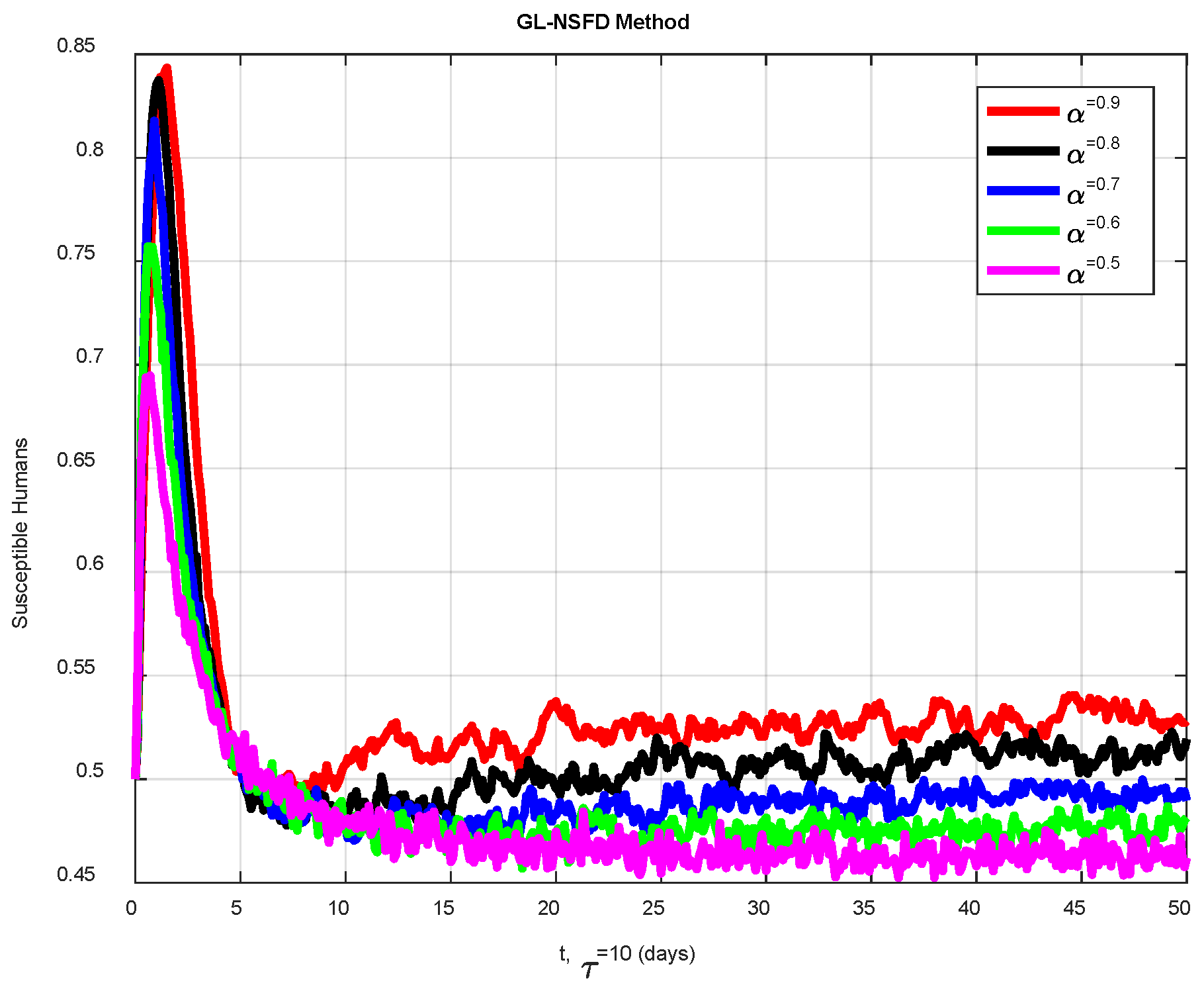
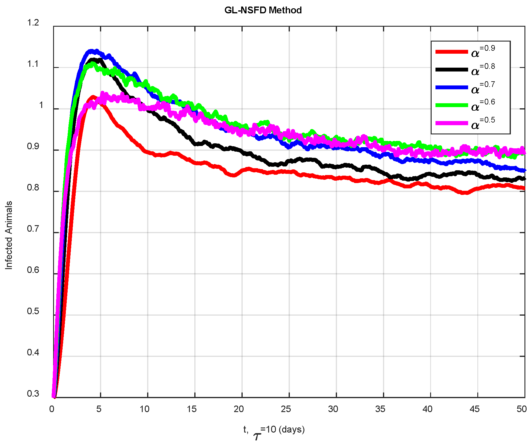
6. Numerical Simulations

The simulations’ parameters are explained in this section. The primary features of the simulated graphs are examined using the set of parametric variables given in

Table 3. Values of parameters.

Parameters	Values	Source [1]
${\mathbf{\Lambda }}_{\mathit{h}}$	$0.5$	Estimated
${\mathbf{\Lambda }}_{\mathit{v}}$	$0.5$	Estimated
${\mathit{\beta }}_{\mathit{h}}$	$1.03$	Fitted
${\mathit{\beta }}_{\mathit{v}}$	$1.04$	Fitted
${\mathit{\mu }}_{\mathit{h}}$	$0.5$	Fitted
${\mathit{\mu }}_{\mathit{v}}$	$0.5$	Estimated
${\mathit{\delta }}_{\mathit{h}}$	$0.001$	Estimated
${\mathit{\delta }}_{\mathit{v}}$	$0.003$	Fitted
${\mathit{\sigma }}_{\mathit{h}}$	$0.004$	Estimated
${\mathit{\sigma }}_{\mathit{v}}$	$0.007$	Fitted
${\mathit{\theta }}_{\mathit{v}}$	0.1	Estimated
$\mathit{\gamma }$	0.001	Fitted
${\mathit{\sigma }}_{\mathit{i}}$	$0\le i\le 1$	Fitted

. Furthermore, these graphs were created at the time when Campylobacteriosis disease was broadly exposed in the human population and finally achieved a stable, present form. Appropriate values of α are selected at the current equilibrium to examine the dynamics of the active cases. The Campylobacteriosis disease model has demonstrated to us that the rates at which the disease spreads vary throughout nations. Since every person or group of people has distinct physical surroundings, health concerns, and other factors, these rates have biological significance.

Discussion

This section provides a detailed explanation of the comparison of the stochastic fractional delayed model at different values of the fractional order $\alpha$ with delay tactics $\left(\tau =10\right)$ on susceptible, infected, and recovered humans and susceptible, infected, and recovered animals. In Figure 3, we show the temporal behavior of the susceptible human population for various values of the fractional order α. The larger the fractional order α is, the system has less memory effects and, therefore, the system is faster. This can create a more protracted decrease in susceptible humans over time, meaning that lower fractional orders may signify a longer period of susceptibility in the populace. Higher fractional orders might indicate a faster transition, which is a result that indicates that we might expect to see more classical, integer-order disease dynamics and a quicker reduction in susceptibility. Figure 4 displays the number of infected humans in different fractional orders α. The lower fractional orders α mean that the infection spreads at a small rate but can stay longer in the system, which causes a wider infection peak. On the other hand, higher fractional orders may exhibit even higher peaks of infections and an even faster decline, meaning faster infection transmission and healing in the population. From this, it can be made out that the fractional order has a direct influence on the time and amplitude of oscillation of the infection wave in humans. In Figure 5, the patterns of recovery of humans are depicted for different values of fractional order α. The rates of recovery decrease with decreasing fractional orders, leading to a delayed increase in the number of recovered individuals and suggesting longer infectious and recovery periods. This could suggest that higher fractional orders may be linked to the rapid aggregation of persons recovered and shorter durations of infectiousness, with a faster recovery period. This means that the memory effect that is contained in fractional orders is central to determining the time that the population takes to recover. In Figure 6, the susceptible animal population is illustrated for different values of the fractional order α. In the same manner, the susceptibility phase is prolonged for lesser fractional orders α in the human population; a similar argument applies to animals and is attributed to slower dynamics, probably due to memory effects where the current state significantly depends upon the past states. Higher fractional orders might indicate a faster decrease in susceptibility, which is in better agreement with traditional disease models, with current statuses impacted less by the previous states. In Figure 7, the number of infected animals with varying fractional orders α is compared. The dynamics of the infected animals portray the contribution of fractional order in the infection spread rate. Hence, lower levels of α are generally associated with lower rising infection rates and longer periods of infection peak width. However, higher fractional orders could denote more precisely the peaks and the decline of the infection, pointing out the increased and speedy dynamics of the disease in these circumstances. Figure 8 presents the analytical results for the recovery of the number for different values of the fractional order α. As earlier observed, lower fractional orders α produce slower recovery rates as well as a later increase in the recovered population. The above shows that at lower fractional dynamics, animals, like human beings, take a longer time than usual to recover from diseases. The result presented shows fractional orders greater than 1 exhibit a higher rate at which recovered animals are been accumulated, suggesting faster recovery from the disease. The graphs show a combined format detailing how the fractional order α affects Campylobacteriosis disease and recovery in both human beings and animals. Smaller fractional order results in longer memory effect and reduced rates of progress as well as recovery, while higher order comes closer to the classical disease rate of change. These effects may give insights into how fractional modeling may more accurately depict real-world diseases where past conditions strongly influence current and future conditions.

7. Conclusions

Probabilistic modeling and the parameter of delayed infection rate are vitally important factors in understanding Campylobacteriosis in populations. The model suggested in the paper provides the means to describe the interaction between the system and the identified factors, as well as the resulting alterations using mathematical analysis and numerical simulations. This is because the numerical solutions attained using the stochastic GL-NSFD scheme have other important characteristics, such as the positivity and boundedness of solutions, which are imperative for any endemic model. The model identifies two equilibrium states: the disease-free equilibrium, in which the Campylobacteriosis rate changes with changes in the public health interventions and behavior; and the endogenous equilibrium, which gives the persistence level of the infection rate in response to the infection transmission dynamics and interventions. Since graphical illustrations assist in identifying situations where the disease indicates equilibrium, which means a continuous interconnected infection, this situation is particularly useful. On the same note, the model shows that an infection-free state is possible if the intervention measures that are recommended are implemented. Our results suggest that increasing the delay parameter and minimizing the memory effect can shift the system dynamics from an endemic state to a disease-free state. In such cases, the effective reproduction number naturally drops below one without altering any other model parameters. The model also looks into the effects of delayed intervention approaches on the incidence of Campylobacteriosis. While the health complications of early intervention in disease are experienced in the form of high incidences of infection, appropriate and aggressive measures (initiation of intervention) offer better ways of minimizing the spread of the disease. This brings the issue of early intervention systems in curbing the spread of Campylobacteriosis into a larger perspective. Applying the same concept to the model, it could be inferred that if strict measures are observed in the model, then the levels of infection in communities could be reduced. Therefore, this stochastic fractional delayed infection model is useful for studying and modeling the impacts and transmission dynamics of Campylobacteriosis in diverse scenarios. Analyzing the delay strategies, the model suggests creating an ideal public health policy and prevention practices. In addition, food hygiene improvement, cementing the safe use of water, targeted vaccination, and other public health measures constitute efficacious control strategies that minimize the spread of Campylobacteriosis.

References

1. Osman, S.; Togbenon, H.A.; Otoo, D. Modelling the dynamics of campylobacteriosis using non finite difference approach with optimal control. Comput. Math. Methods Med. 2020, 2020, 8843299. [Google Scholar] [CrossRef]
2. Chuma, F.M.; Ngailo, E.K. Mathematical analysis of campylobacteriosis disease model in human with saturated incidence rate and treatment. Math. Open 2024, 3, 2350011. [Google Scholar] [CrossRef]
3. Iacono, G.L.; Cook, A.J.C.; Derks, G.; Fleming, L.E.; French, N.; Gillingham, E.L.; Villeta, L.C.G.; Heaviside, C.; La Ragione, R.M.; Leonardi, G.; et al. A mathematical, classical stratification modeling approach to disentangling the impact of weather on infectious diseases: A case study using spatio-temporally disaggregated Campylobacter surveillance data for England and Wales. PLoS Comput. Biol. 2024, 20, e1011714. [Google Scholar] [CrossRef] [PubMed]
4. Dzianach, P.A.; Dykes, G.A.; Strachan, N.J.; Forbes, K.J.; Pérez-Reche, F.J. Unveiling the Mechanisms for Campylobacter jejuni Biofilm Formation Using a Stochastic Mathematical Model. Hygiene 2024, 4, 326–345. [Google Scholar] [CrossRef]
5. Carvalho, D.; Chitolina, G.Z.; Wilsmann, D.E.; Lucca, V.; Emery, B.D.D.; Borges, K.A.; Furian, T.Q.; Santos, L.R.D.; Moraes, H.L.D.S.; Nascimento, V.P.D. Development of Predictive Modeling for Removal of Multispecies Biofilms of Salmonella Enteritidis, Escherichia coli, and Campylobacter jejuni from Poultry Slaughterhouse Surfaces. Foods 2024, 13, 1703. [Google Scholar] [CrossRef] [PubMed]
6. Holmes, J. Understanding How Mutability Facilitates Survival of Alternating Selection and Bottlenecks by the Major Food-Borne Pathogen Campylobacter jejuni. Ph.D. Dissertation, University of Leicester, Leicester, UK, 2024. [Google Scholar]
7. Sahin, O.; Pang, J.; Pavlovic, N.; Tang, Y.; Adiguzel, M.C.; Wang, C.; Zhang, Q. A Longitudinal Study on Campylobacter in Conventionally Reared Commercial Broiler Flocks in the United States: Prevalence and Genetic Diversity. Avian Dis. 2024, 67, 317–325. [Google Scholar] [CrossRef] [PubMed]
8. Braga, P.F.D.S. Enhancing the control of Campylobacter jejuni in a Theragnostic Approach: FTIR-ATR Combined with Artificial Intelligence, Binding-Peptides, and the Use of Chicken Embryos as an In Vivo Model. Ph.D. Thesis, Universidade Federal de Uberlândia, Uberlândia, Brazil, 2024. [Google Scholar]
9. Sinha, R.; LeVeque, R.M.; Callahan, S.M.; Chatterjee, S.; Stopnisek, N.; Kuipel, M.; Johnson, J.G.; DiRita, V.J. Gut metabolite L-lactate supports Campylobacter jejuni population expansion during acute infection. Proc. Natl. Acad. Sci. USA 2024, 121, e2316540120. [Google Scholar] [CrossRef] [PubMed]
10. Alghamdi, M.A.; Azam, F.; Alam, P. Deciphering Campylobacter jejuni DsbA1 protein dynamics in the presence of anti-virulent compounds: A multi-pronged computer-aided approach. J. Biomol. Struct. Dyn. 2024, 1–17. [Google Scholar] [CrossRef] [PubMed]
11. Knipper, A.D.; Plaza-Rodríguez, C.; Filter, M.; Wulsten, I.F.; Stingl, K.; Crease, T. Modeling the survival of Campylobacter jejuni in raw milk considering the viable but non-culturable cells (VBNC). J. Food Saf. 2023, 43, e13077. [Google Scholar] [CrossRef]
12. Brinch, M.L.; Hald, T.; Wainaina, L.; Merlotti, A.; Remondini, D.; Henri, C.; Njage, P.M.K. Comparison of source attribution methodologies for human campylobacteriosis. Pathogens 2023, 12, 786. [Google Scholar] [CrossRef] [PubMed]
13. Soto-Beltrán, M.; Lee, B.G.; Amézquita-López, B.A.; Quiñones, B. Overview of methodologies for the culturing, recovery and detection of Campylobacter. Int. J. Environ. Health Res. 2023, 33, 307–323. [Google Scholar] [CrossRef] [PubMed]
14. Said, Y.; Singh, D.; Sebu, C.; Poolman, M. A novel algorithm to calculate elementary modes: Analysis of Campylobacter jejuni metabolism. Biosystems 2023, 234, 105047. [Google Scholar] [CrossRef] [PubMed]
15. Myintzaw, P.; Jaiswal, A.K.; Jaiswal, S. A review on campylobacteriosis associated with poultry meat consumption. Food Rev. Int. 2023, 39, 2107–2121. [Google Scholar] [CrossRef]
16. Bodie, A.R.; Rothrock Jr, M.J.; Ricke, S.C. Comparison of optical density-based growth kinetics for pure culture Campylobacter jejuni, coli and lari grown in blood-free Bolton broth. J. Environ. Sci. Health Part B 2023, 58, 671–678. [Google Scholar] [CrossRef] [PubMed]
17. Rousou, X.; Furuya-Kanamori, L.; Kostoulas, P.; Doi, S.A. Diagnostic accuracy of multiplex nucleic acid amplification tests for Campylobacter infection: A systematic review and meta-analysis. Pathog. Glob. Health 2023, 117, 259–272. [Google Scholar] [CrossRef] [PubMed]
18. Hendrickson, S.M.; Thomas, A.; Raué, H.P.; Prongay, K.; Haertel, A.J.; Rhoades, N.S.; Slifka, J.F.; Gao, L.; Quintel, B.K.; Amanna, I.J.; et al. Campylobacter vaccination reduces diarrheal disease and infant growth stunting among rhesus macaques. Nat. Commun. 2023, 14, 3806. [Google Scholar] [CrossRef] [PubMed]
19. Knipper, A.D.; Göhlich, S.; Stingl, K.; Ghoreishi, N.; Fischer-Tenhagen, C.; Bandick, N.; Tenhagen, B.A.; Crease, T. Longitudinal study for the detection and quantification of Campylobacter spp. in dairy cows during milking and in the dairy farm environment. Foods 2023, 12, 1639. [Google Scholar] [CrossRef] [PubMed]
20. Kingsbury, J.M.; Horn, B.; Armstrong, B.; Midwinter, A.; Biggs, P.; Callander, M.; Mulqueen, K.; Brooks, M.; van der Logt, P.; Biggs, R. The impact of primary and secondary processing steps on Campylobacter concentrations on chicken carcasses and portions. Food Microbiol. 2023, 110, 104168. [Google Scholar] [CrossRef] [PubMed]
21. Sene, N. Analysis of the stochastic model for predicting the novel coronavirus disease. Adv. Differ. Equ. 2020, 2020, 568. [Google Scholar] [CrossRef] [PubMed]
Figure 1. Graphical map of the Campylobacteriosis disease model.
Fractalfract 09 00358 g001
Figure 2. Sensitivity indices of reproduction number R 0 .
Fractalfract 09 00358 g002
Figure 3. Susceptible humans are shown graphically for different values of the fractional order α.
Fractalfract 09 00358 g003
Figure 4. Infected humans are shown graphically for different values of the fractional order α.
Fractalfract 09 00358 g004
Figure 5. Recovered humans’ graphical behavior for different values of fractional order α.
Fractalfract 09 00358 g005
Figure 6. Susceptible animals’ graphical behavior for different values of fractional order α.
Fractalfract 09 00358 g006
Figure 7. Infected animals’ graphical behavior for different values of fractional order α.
Fractalfract 09 00358 g007
Figure 8. Recovered animals’ graphical behavior for different values of fractional order α.
Fractalfract 09 00358 g008