Dissipativity Constraints in Zener-Type Time Dispersive Electromagnetic Materials of the Fractional Type

Abstract

Thermodynamic constraints must be satisfied for the parameters of a constitutive relation, particularly for a model describing an electromagnetic (or any other) material with the intention of giving that model a physical meaning. We present sufficient conditions for the parameters of the constitutive relation of an electromagnetic Zener-type fractional 2D and 3D anisotropic model so that a weak form of the thermodynamic (entropy) inequality is satisfied. Moreover, for such models, we analyze the corresponding thermodynamic constraints for field reconstruction and regularity in the 2D anisotropic case. This is carried out by the use of the matrix version of the Bochner theorem in the most general form, including generalized functions as elements of a matrix, which appear in that theorem. The given numerical results confirm the calculus presented in the paper.

1. Introduction

In this paper, we investigate constitutive relations utilizing fractional derivatives in the modeling of linear time-dispersive electromagnetic materials related to anisotropic non-homogeneous and homogeneous characteristics with respect to the third dimension. For 3D homogeneous material with respect to the third dimension, we can omit the third dimension from further analysis as the convolution kernel can be represented by a block diagonal matrix, where the first block is a 2 × 2 matrix representing a 2D convolution kernel and the second block is a constant scalar. Therefore, without loss of generality, this case can be treated as 2D, i.e., a 2D material; moreover, our general results include bianisotropic materials.

It is well-known that dispersivity reflects frequency dependence, i.e., time-memory effects and space-nonlocality effects in electromagnetic materials. For example, with regard to time dispersivity, in real dielectric materials, a polarization process cannot occur instantaneously since there is a frequency dependence of the dielectric permittivity $\epsilon \left(\omega \right)$, which in many applications, could not be neglected [1]. In addition, in real magnetic materials, polarization, magnetization, and current density cannot follow the rapid change in the electromagnetic field. However, for metals, both dispersion and dissipation must be considered, as their respective contributions vary significantly with the frequency of the electromagnetic field [2]. Note that electromagnetic materials and metamaterials (which are, necessarily, frequency dissipative [3]) have recently gained a lot of attention; therefore, their dissipation properties are interesting for investigation. Let us mention a few papers. Some simple models are initially proposed in [4]. Using Fourier series expansions, certain necessary entropy (i.e., dissipativity) restrictions on the corresponding constitutive parameters are provided in [3] under the assumption of a small frequency bandwidth. Recently, memory and non-local effects in electromagnetic metamaterials were treated in [5,6]. In [7], the author investigated the time evolution of fractional electromagnetic waves using time-fractional Maxwell equations. Moreover, in [8], the same author applied the developed theory to the modeling of electromagnetic metamaterials, where the fractional model was introduced by the direct fractionalization of Maxwell equations.

Various mathematical approaches in modeling based on memory-dependent properties of materials are presented in [9,10,11], while some recent results can be found in [12,13,14]. For example, in [9], the general constitutive relations for linear time-dispersive electromagnetic materials are introduced in the classical sense (continuous kernels), including anisotropic and bianisotropic ones, and necessary conditions for the Clausius–Duhem inequality to hold in the isothermal case. A somewhat similar analysis is provided in [10,11]. In [13], viscoferromagnetic materials represented by an isotropic nonlocal constitutive equation are considered, where a simple fractional constitutive relation is postulated using the fractional derivative of Caputo. Also, in [15], the authors analyzed an electromagnetic field in a conducting medium, modeled by isotropic Ohm’s law, of both the fractional integral and derivative (Caputo) type, with emphasis on the solution of Maxwell equations for the mentioned medium. In [16], generalized isotropic constitutive equations in terms of fractional Riemann–Liouville derivatives are introduced in Maxwell’s equations for various elements of electrical circuits.

All existing materials in nature (including electromagnetic materials) must satisfy the second law of thermodynamics. The fulfillment of derived thermodynamic conditions and constraints, therefore, guarantees that the obtained model can correspond to some real material present in nature. It means that in any process concerning any particular material, there must be a dissipation of energy (see [17,18,19]). It also means that a set of measurement data can be approximated with a curve that minimizes least squares but presents a solution that is not physically admissible. Similarly to [20] for viscoelastic materials, by using thermodynamic restrictions, i.e., constraints on the parameters of a model for some “real-world” electromagnetic material, one can perform constrained optimization in order to ensure a physically admissible solution to the parameters of the model. In the literature, one cannot find a sufficiently developed analysis related to the characterization of thermodynamic properties in terms of sufficient conditions for the dissipativity of dispersive electromagnetic materials, i.e., for the second law of thermodynamics expressed through the Clausius–Duhem inequality. This is especially the case with kernels of the distributive type, which model the dispersivity of anisotropic and bianisotropic materials. This is mostly because the matrix-valued generalization of the Bochner–Schwartz theorem (distributional case) is not present in the existing literature to the best of the authors’ knowledge. Refs. [10,11,18] were among the first to tackle the classical case (C, $L^1$, or $L^2$), but they did not consider any particular known fractional model or distributional-type kernels. Moreover, analysis of the mentioned thermodynamic constraints is particularly lacking for fractional models, especially of the anisotropic type. Our paper aims to establishing such sufficient conditions, where we provide a generalization in terms of sufficient conditions for the Clausius–Duhem inequality to hold for anisotropic and bi-anisotropic distribution-type kernels. We additionally obtain such thermodynamic constraints on parameters of generalized fractional Zener-type anisotropic constitutive relations.

Concerning the fractional calculus used in this paper, we note that for electromagnetic materials, concerning the second law of thermodynamics, such an approach was only recently addressed in [13], where a simple fractional model expressing the time dispersivity of the constitutive relation was analyzed. In the framework of fractional viscoelasticity, this would be a fractional generalization of Hooke’s Law. In addition, complex models are also invoked in the literature. On the other hand, fractional calculus is widely involved in the modeling of non-local properties of linear viscoelastic materials in time and space in terms of various constitutive relations [21,22,23] with restrictions to the coefficients obtained by the use of the one-dimensional Bochner–Schwarz case for the Clausius–Duhem thermodynamic inequality, where convolution-type kernels (such as the generalized fractional Zener type) are included. In [21], sufficient thermodynamic constraints are provided on parameters of a particular one-dimensional convolution kernel of the distributional fractional type (the generalized Burgers model). This approach involves weaker restrictions, which means more general conditions on the solvability of the corresponding wave equation compared to recent results based on the Bagley–Torvik approach [23].

In this paper, we utilize the matrix-valued generalization of the Bochner theorem and extend its application to the tempered distributional case to deliver sufficient conditions for the dissipativity of anisotropic and bianisotropic electromagnetic materials, i.e., for the Clausius–Duhem thermodynamic inequality to hold under isothermal conditions. Such conditions are provided for general distribution-type anisotropic and bianisotropic kernels and then also in the form of restrictions on the parameters of constitutive relations for Zener-type fractional models in both non-homogeneous 2D and 3D anisotropic cases. The results in both cases are novel. In contrast to [21], distribution-type kernels are anisotropic and bianisotropic, so the matrix-valued generalization of the Bochner theorem to the mentioned distribution case must be utilized. In addition, electromagnetic material is modeled instead of viscoelastic material. We also provide connections between the restrictions on the parameters of the given fractional Zener-type anisotropic model in the 2D case and the existence and regularity of the solution for the inverse problem of reconstructing the electric field, given the current density for the 2D case, on the rectangular domain. In the final part of the paper, we present some numerical results.

2. Preliminary

2.1. Notation and Framework

$L^1({\mathbb{R}}^d\times {\mathbb{R}}_{+})$ is denoted as the space a. of integrable functions with a value of $\mathbb{C}$ (complex numbers) over the product of the Euclidean d-dimensional space ${\mathbb{R}}^d$ and ${\mathbb{R}}_{+}=[0,\infty )$. It is said that $f\in L^1({\mathbb{R}}^d\times {\mathbb{R}}_{+})$ is supported by ${\mathbb{R}}^3\times [0,T]$ if $f=0$ out of ${\mathbb{R}}^d\times [0,T],T>0.$ Convolution of $f,g\in L^1({\mathbb{R}}^d\times {\mathbb{R}}_{+})$ with respect to t is defined as $f{\ast }_{t}g={\int }_0^{\infty }f(x,u)g(x,t-u)du,x\in {\mathbb{R}}^d,t\in [0,\infty ]$. In the sequel, all the convolutions will be defined with respect to t, so we will write ∗ instead of ${\ast }_t$. Concerning the Schwartz distribution theory [24,25], recall that $\mathcal{S}\left({\mathbb{R}}^d\right)$ denotes the space of rapidly decreasing functions; a smooth function (infinitely times differentiable) $\varphi \in \mathcal{S}\left({\mathbb{R}}^d\right)$ if ${(1+|x\left|\right)}^p{\partial }^{\alpha }\varphi \left(x\right)|<\infty$, $x\in {\mathbb{R}}^d$ $\left|\alpha \right|\le q$, and $\alpha ={\alpha }_1+...+{\alpha }_d$ for all non-negative integers p and q ($p,q\in {\mathbb{N}}_0$); ${\mathcal{S}}^{\prime }\left(\mathbb{R}\right)$ is its dual, i.e., the space of tempered distributions. We specify tempered measures as continuous functionals over the test space consisting of continuous functions $\varphi$ with the properties ${(1+|x\left|\right)}^p\varphi \left(x\right)<\infty$, $x\in {\mathbb{R}}^d$, and $p\in {\mathbb{N}}_0$. ${\mathcal{S}}^{\prime }({\mathbb{R}}^d\times {\mathbb{R}}_{+})$ is denoted as the space of distribution in ${\mathcal{S}}^{\prime }\left({\mathbb{R}}^{d+1}\right)$ supported by ${\mathbb{R}}^d\times [0,\infty ),$ which means that a tempered distribution of $f\in {\mathcal{S}}^{\prime }\left({\mathbb{R}}^{d+1}\right)$ equals zero over the test functions supported in ${\mathbb{R}}^d\times (-\infty ,0)$. Especially in the one-dimensional case, for the space of tempered distributions on $\mathbb{R}$ supported by ${\mathbb{R}}_{+}$, we use the notation ${\mathcal{S}}_{+}^{\prime }$. The Fourier transform $\mathcal{F}:\mathcal{S}\left(\mathbb{R}\right)\to \mathcal{S}\left(\mathbb{R}\right)$ is defined as $\mathcal{F}\left(\phi \right)\left(\omega \right)=\widehat{\phi }\left(\omega \right)={\int }_{{\mathbb{R}}^d}\phi \left(t\right)e^{-i\omega t}dt$, $\omega \in \mathbb{R}$, and $\phi \in \mathcal{S}\left(\mathbb{R}\right)$. For $u\in {\mathcal{S}}^{\prime }\left(\mathbb{R}\right)$, its Fourier transform $\mathcal{F}:{\mathcal{S}}^{\prime }\left(\mathbb{R}\right)\to {\mathcal{S}}^{\prime }\left(\mathbb{R}\right)$ is defined by the following duality: $\langle \langle \mathcal{F},\phi \rangle \rangle \left(\omega \right)=\langle \langle u,\mathcal{F}\left(\phi \right)\left(\omega \right)\rangle \rangle ,\phi \in \mathcal{S}\left(\mathbb{R}\right)$, $\omega \in \mathbb{R}$, where $\langle \langle ·,·\rangle \rangle$ denotes dual pairing, i.e., the action of a distribution u on a test function $\phi$. Recall, $u(x,t)\in {\mathcal{S}}^{\prime }({\mathbb{R}}^d\times \mathbb{R})$ is even in t if $\check{u}=u$ and odd in t if $\check{u}=-u$, where $\langle \langle \check{u},\phi \rangle \rangle =\langle \langle u,\check{\phi }\rangle \rangle$, $\phi \in \mathcal{S}\left(\mathbb{R}\right),$ $\check{\phi }\left(t\right)=\phi (-t)$, and $t\in \mathbb{R}$. Also, $u(x,t)\in {\mathcal{S}}^{\prime }({\mathbb{R}}^d\times \mathbb{R})$ is a non-negative definite in t if for every $x\in {\mathbb{R}}^d$, it holds $\langle \langle u(x,t),\phi \ast {\phi }^{\ast }\left(t\right)\rangle \rangle ={\int }_{-\infty }^{\infty }\langle \langle u(x,t-\tau ),\phi \left(\tau \right)\rangle \rangle \overline{\phi \left(t\right)}dt\ge 0$ for any $\phi \in \mathcal{S}\left(\mathbb{R}\right)$, where ${\phi }^{\ast }=\overline{\breve{\phi }}$ (bar means conjugation). The Bochner–Schwartz theorem (see [25,26]) states that a tempered distribution $u(x,t)\in {\mathcal{S}}^{\prime }({\mathbb{R}}^d\times \mathbb{R})$ is a non-negative definite in t if it is the Fourier transform of a non-negative tempered measure in t for every $x\in {\mathbb{R}}^d$. The extension of the definition of non-negativity for a $p\times p$ matrix-valued tempered distribution, i.e., an element of ${\left({\mathcal{S}}^{\prime }({\mathbb{R}}^d\times \mathbb{R})\right)}^{p\times p}$, $p\in \mathbb{N}$, as shown in [25], reads as follows: symmetric matrix $f\in {\left({\mathcal{S}}^{\prime }({\mathbb{R}}^d\times \mathbb{R})\right)}^{p\times p}$ (meaning that $f^H=f$, where ${(·)}^H={\overline{(·)}}^T$ and ${(·)}^T$ denotes the transposition of a matrix) is a non-negative definite matrix-valued distribution in t if for every $x\in {\mathbb{R}}^d$ the terms of the matrix satisfy the following:

$$\sum _{i,j=1}^p{\int }_{{\mathbb{R}}^d}\langle \langle f_{ij}(x,t-\tau ),{\phi }_i\left(\tau \right)\rangle \rangle \overline{{\phi }_j\left(t\right)}dt\ge 0,\mathrm{f}\mathrm{o}\mathrm{r} \mathrm{a}\mathrm{n}\mathrm{y}\phi \left(t\right)=({\phi }_1\left(t\right),\dots ,{\phi }_p\left(t\right))\in {\left(\mathcal{S}\left(\mathbb{R}\right)\right)}^p.$$

We recall the extension of the Bochner’s theorem for the matrix-valued case ([27], Theorem 3.8, p. 78):

(∗) Let $a(x,t),\widehat{a}(x,\xi )\in {\left(L^1({\mathbb{R}}^d\times \mathbb{R})\right)}^{p\times p}$. Then, Bochner’s theorem for the matrix-valued case asserts the following: $a(x,t)$ is a positive definite function in t (for every $x\in {\mathbb{R}}^d$) if $\widehat{a}(x,\xi )$, and $\xi \in \mathbb{R}$ is a self-adjoint positive definite matrix function in ξ (for every $x\in {\mathbb{R}}^d$). In that case, we use the notation $\widehat{a}⪰0$.

We define the Laplace transform as $\tilde{u}$ for $u\in L^1\left(\mathbb{R}\right)$, supported by $[0,\infty )$ so that $\left|u\left(t\right)\right|\le A{e}^{at}$, $a\ge 0$, and $A>0$ (u is called exponentially bounded), as $\mathcal{L}\left(u\right)\left(t\right)=\tilde{u}\left(s\right)={\int }_0^{\infty }u\left(t\right)e^{-st}dt$ and $\mathrm{Re}s>a$; $\tilde{u}\left(s\right),s\in \mathbb{C},\mathrm{Re}s>a,$ is a holomorphic function. For $u\in {\mathcal{S}}^{\prime }({\mathbb{R}}^d\times {\mathbb{R}}_{+}),$ the Laplace transform with respect to t ($x\in {\mathbb{R}}^d$) is defined as $\mathcal{L}\left(u\right)(x,s)=\left(\tilde{u}(x,t)\right)\left(s\right)=\left(\mathcal{F}\left(e^{\eta t}u(x,t)\right)\right)\left(\xi \right)$ and $s=\xi +i\eta \in {\mathbb{C}}_{+}={\mathbb{R}}_{+}+i\mathbb{R}$. It is a holomorphic function in s. Conversely, under appropriate assumptions on a holomorphic functions $U\left(s\right)$, $s\in \mathbb{C}$, and $\mathrm{Re}s>a>0$, it holds that $u\left(t\right)={\displaystyle \frac{1}{2\pi i}}{\int }_{{\sigma }_0-i\infty }^{{\sigma }_0+i\infty }U\left(s\right)e^{st}ds$ and $t>0$ for any fixed ${\sigma }_0>a$, and that u is an exponentially bounded function.

We finish this section with the Caputo fractional derivatives. $\theta$ is denoted as the Heaviside function (which is equal to the characteristic function of $[0,\infty )$). Its distributional derivative is a delta distribution $\delta \left(t\right),t\in \mathbb{R}.$ Further, let $f_{\alpha }\left(t\right)={\displaystyle \frac{t_{+}^{-\alpha }}{\Gamma (1-\alpha )}}$, $t_{+}^{-\alpha }=\theta \left(t\right)t^{-\alpha }$, $t\in \mathbb{R}$, and $\alpha \in (0,1)$ ($\Gamma$ is the Gamma function). Then, for $u\in {\mathcal{S}}^{\prime }({\mathbb{R}}^d\times {\mathbb{R}}_{+})$, the Caputo fractional derivative with respect to t of order $\alpha \in (0,1)$ (in the sense of distributions) is defined by the following:

$$u^{\left(\alpha \right)}(x,t)=f_{\alpha }\left(t\right)\ast u(x,t),t>0,x\in {\mathbb{R}}^d.$$

It belongs to ${\mathcal{S}}^{\prime }({\mathbb{R}}^d\times {\mathbb{R}}_{+})$. $A{C}_{loc}({\mathbb{R}}^d\times [0,\infty ))$ is denoted as the space of continuous functions u, which is absolutely continuous on $[0,A]$ with respect to t, with derivatives with respect to the t integrable on $[0,A]$, and with respect to t for every $A>0$ and $x\in {\mathbb{R}}^d$. If $u\in A{C}_{loc}({\mathbb{R}}^d\times [0,\infty ))$, $\alpha \in (0,1)$; then,

$$u^{\left(\alpha \right)}(x,t)={\displaystyle \frac{1}{\Gamma (1-\alpha )}}{\int }_0^t{\displaystyle \frac{u^{\prime }(x,\tau )}{{(t-\tau )}^{\alpha }}}d\tau ,t\in [0,\infty ),x\in {\mathbb{R}}^d,$$

(1)

where $u^{\prime }$ is the first derivative of function u, while $\Gamma$ is the Gamma function. The term $u^{\left(\alpha \right)}(x,t)$ in (1) is bound for almost all $t\in {\mathbb{R}}_{+}$ for every $x\in {\mathbb{R}}^d$.

Remark 1. 

In the sequel, all the actions on functions and distributions defined over ${\mathbb{R}}^d\times {\mathbb{R}}_{+}$ are performed on the variable $t\in \mathbb{R}$ so that $x\in {\mathbb{R}}^d$ can be considered a parameter and even neglected. But, some functions or distributions depend only on t. So, to exclude confusion in the notation, we will not neglect x.

If $h(x,t)\in {\mathcal{S}}^{\prime }({\mathbb{R}}^d\times {\mathbb{R}}_{+})$ is continuous with respect to $x\in {\mathbb{R}}^d$, then we know that there exists $F(x,t)$ continuous in x and integrable with respect to $t\in [0,\infty )$, and there exists $m\in {\mathbb{N}}_0$ so that $h(x,t)={\left({\displaystyle \frac{d}{dt}}\right)}^{m}F(x,t)$. In this case, $\mathcal{F}\left(h(x,t)\right)(x,\omega )={\left(i\omega \right)}^m{\int }_0^{\infty }F(x,t)e^{-i\omega t}dt$.

2.2. Constitutive Relations and Dissipativity of the Dispersive Electromagnetic Materials

Recall the well-known system of Maxwell’s partial differential equations for macroscopic electromagnetic fields in a dimensionless form:

$$\begin{array}{ccc}\hfill & & \nabla \times E(x,t)=-{\partial }_{t}B(x,t),\hfill \\ & & \nabla \times H(x,t)=J(x,t)+{\partial }_{t}D(x,t),t>0,x\in \Omega ,\hfill \end{array}$$

(2)

where ${\partial }_t$ denotes the partial derivative with respect to t, $\nabla =\left({\partial }_{x_1},{\partial }_{x_2},{\partial }_{x_3}\right)$ denotes the gradient, $E={(E_1,E_2,E_3)}^T$ (vector column) is the electric field, $H={(H_1,H_2,H_3)}^T$ is the magnetic field, $B={(B_1,B_2,B_3)}^T$ is the magnetic induction field, $D={(D_1,D_2,D_3)}^T$ is the electric displacement field, and $J={(J_1,J_2,J_3)}^T$ is the current density. Recall that the cross product in (2) is defined by $\nabla \times E=({\partial }_{x_2}{E}_3-{\partial }_{x_3}{E}_2,{\partial }_{x_3}{E}_1-{\partial }_{x_1}{E}_3,{\partial }_{x_1}{E}_2-{\partial }_{x_2}{E}_1)$. This system is completed by additional constitutive relations, which connect the mentioned fields through scalar functions $D=D(E,H)$, $B=B(E,H)$, and $J=J\left(E\right)$ over a specified domain (open or close connected set) $\Omega \subset {\mathbb{R}}^3$. We assume that E and H are continuous on $\Omega \times [0,\infty )$ and that $E(x,·),H(x,·)$ are supported by $[0,\infty )$ for all $x\in \Omega$ ($E,H\in C(\Omega \times {\mathbb{R}}_{+})$). If the medium is a vacuum, constitutive relations are provided as $D={\epsilon }_{0}E$ and $B={\mu }_{0}H$, where positive constants ${\epsilon }_0$ and ${\mu }_0$ are the vacuum permittivity and permeability constants, respectively. Note that constitutive relations describe electromagnetic media, i.e., materials themselves. They are independent in relation to the Maxwell equations provided by (2). In this paper, we consider electromagnetic materials with constitutive relations described by certain time-invariant and causal linear operators. Such operators can be defined (see [25]) by convolution kernels Q and G as follows.

Let e be a vector column, Q a matrix of format $6\times 6$, and $E,H,D,$ and B vector columns of the $3\times 1$ format:

$$\begin{array}{ccc}\hfill & & e=\left[\begin{array}{c}E\\ H\end{array}\right],Q=\left[\begin{array}{cc}{Q}_{de}& Q_{dh}\\ Q_{be}& Q_{bh}\end{array}\right],Q{\ast }_{t}e=\left[\begin{array}{c}D\\ B\end{array}\right].\hfill \end{array}$$

(3)

Here, $Q\ast e={\left({\sum }_{j=1}^6{Q}_{1j}\left(t\right){\ast }_t{e}_j(x,t),\dots ,{\sum }_{j=1}^6{Q}_{6j}\left(t\right){\ast }_t{e}_j(x,t)\right)}^T$. We impose the condition that Q is a symmetric matrix, which is equivalent to ${\left(Q_{de}\right)}^T=Q_{de}$, ${\left(Q_{bh}\right)}^T=Q_{bh}$, and $Q_{dh}=Q_{be}$. In addition, we assume that G is a symmetric matrix.

The constitutive relations have the following form:

$$\begin{array}{ccc}\hfill & & D(x,t)=Q_{de}\left(t\right)\ast E(x,t)+Q_{dh}\left(t\right)\ast H(x,t),\hfill \\ & & B(x,t)=Q_{be}\left(t\right)\ast E(x,t)+Q_{bh}\left(t\right)\ast H(x,t),\hfill \\ & & J(x,t)=G\left(t\right)\ast E(x,t),t>0,x\in \Omega \subset {\mathbb{R}}^3,\hfill \end{array}$$

(4)

where kernels are matrices $Q_{ab}\in {\left({\mathcal{S}}_{+}^{\prime }\right)}^{3\times 3}$ and $ab\in \{de,dh,be,bh\}$, and $G\in {\left({\mathcal{S}}_{+}^{\prime }\right)}^{3\times 3}$ depend only on time t; $Q_{ab}\in {\left({\mathcal{S}}_{+}^{\prime }\right)}^{3\times 3}$ means that $Q_{ab}^{ij}\in {\mathcal{S}}_{+}^{\prime }$ for all $i,j=1,2,3$ (the same for G). Also, we use the following notation:

$$\begin{array}{ccc}\hfill Q_{ab}\left(t\right)\ast W{(x,t)}^T& =& \left(\sum _{j=1}^3{Q}_{ab}{\left(t\right)}^{1j}\left(t\right)\ast W_j(x,t),\sum _{j=1}^3{Q}_{ab}{\left(t\right)}^{2j}\left(t\right)\ast W_j(x,t),\right.\hfill \\ & & {\left.\sum _{j=1}^3{Q}_{ab}{\left(t\right)}^{3j}\left(t\right)\ast W_j(x,t)\right)}^T,x\in \Omega ,t>0,\hfill \end{array}$$

for $ab\in \{de,dh,be,bh\}$ and $W\in \{E,H\}$, as well as

$$\begin{array}{ccc}\hfill G\left(t\right)\ast E{(x,t)}^T& =& \left(\sum _{j=1}^{3}G{\left(t\right)}^{1j}\left(t\right)\ast E_j(x,t),\sum _{j=1}^{3}G{\left(t\right)}^{2j}\left(t\right)\ast E_j(x,t),\right.\hfill \\ & & {\left.\sum _{j=1}^{3}G{\left(t\right)}^{3j}\left(t\right)\ast E_j(x,t)\right)}^T,x\in \Omega ,t>0.\hfill \end{array}$$

The system (4) models the most general linear time-dispersive bianisotropic electromagnetic material (see [9]). Recall that, in the case when kernels $Q_{ab}$ (for all $ab$) and G are diagonal matrices, the material is called isotropic, while in the case $Q_{dh}=Q_{be}=0$, while $Q_{ab}$ and G are not diagonal, the material is called anisotropic.

We now consider an electromagnetic system with a uniform mass density, which occupies the region $\Omega \subset {\mathbb{R}}^3$ with a smooth boundary. Let us assume that the process is isothermal in $[0,T_0]$ for arbitrary but fixed $T_0>0$. This means that the temperature $\eta \left(t\right)$, $t>0,$ of the electromagnetic system is constant. Moreover, we assume that the process is cyclic with respect to the virginal state. This means that

$$E(x,0)=E(x,T_0)=0,H(x,0)=H(x,T_0)=0,x\in \Omega .$$

(5)

Then, the second law of thermodynamics for electromagnetic materials is equivalent (see [18]) to the Clausius–Duhem inequality.

$$\begin{array}{ccc}\hfill & & {\int }_{\Omega }{\int }_0^{T_0}\left(\langle {\partial }_{t}D(x,t),E(x,t)\rangle +\langle {\partial }_{t}B(x,t),H(x,t)\rangle +\langle J(x,t),E(x,t)\rangle \right)dxdt\ge 0,\hfill \end{array}$$

(6)

where $\langle ·,·\rangle$ denotes the scalar product in ${\mathbb{R}}^3$.

Proposition 1. 

If one assumes that the Clausius–Duhem inequality (the CD inequality in the sequel) (6) holds for every open ${\Omega }_1\subset \Omega$, and that $E,{\partial }_{t}D,H,{\partial }_{t}B$ and J are continuous on ${\Omega }_1\times {\mathbb{R}}_{+}$ and have a discrete set of zeros (zeros do not have accumulation points, i.e., they are isolated), then we can assume that the integrand with respect to x is positive because, in this case, (6) is equivalent to the following:

$$\begin{array}{ccc}\hfill & & {\int }_0^{T_0}\left(\langle {\partial }_{t}D(x,t),E(x,t)\rangle +\langle {\partial }_{t}B(x,t),H(x,t)\rangle +\langle J(x,t),E(x,t)\rangle \right)dt\ge 0.\hfill \end{array}$$

(7)

Remark 2. 

We will analyze the sufficient condition for the CD inequality considering (7) in a more general setting of distributions, which means that integration with respect to t will be considered as a dual pairing.

For the sake of simplicity, we will usually take $\Omega ={\mathbb{R}}^3$.

3. Thermodynamic Restrictions

3.1. General Results

We first present some general results for the convolution kernel figuring in the constitutive relations of electromagnetic materials provided by (4). Our general assumption for e provided by (3) is as follows:

$$\left(C1\right)e\in {\left(C_0^1({\mathbb{R}}^3\times [0,T_0])\right)}^6,T_0>0,$$

where $C_0^1({\mathbb{R}}^3\times [0,T_0])$ is the space of functions with the continuous first derivative with respect to t on $[0,T_0]$ supported by ${\mathbb{R}}^3\times [0,T_0]$, meaning that $e_1\dots ,e_6$ are defined over ${\mathbb{R}}^3\times \mathbb{R}$ and equal zero over ${\mathbb{R}}^3\times ((-\infty ,0)\cup (T_0,\infty ))$. It is obvious that the following holds.

Proposition 2. 

Under the assumptions of Proposition 1, the sufficient conditions for the thermodynamic inequality (7), and thus for the CD inequality (6), are as follows:

$${\int }_0^{T_0}\langle e(x,·),{\partial }_t(Q(·)\ast e(x,·))\left(t\right)\rangle dt\ge 0,{\int }_0^{T_0}\langle E((x,t),(G\ast E(x,·))\left(t\right)\rangle dt\ge 0(x\in {\mathbb{R}}^3).$$

(8)

As we noted in Remark 2, in the sequel, we will assume that the integration with respect to t is understood in the sense of dual pairing since we will assume that the elements of matrix Q are tempered distributions.

We rewrite the integrals in (8) as follows:

$$\begin{array}{ccc}\hfill & & {\int }_0^{T_0}\langle e(x,t),{\partial }_t(Q\ast e(x,·))\left(t\right)\rangle dt={\int }_0^{T_0}{\int }_0^t\langle e(x,t),{\displaystyle \frac{d}{dt}}Q(t-m)e(x,m)\rangle dmdt\hfill \\ & & ={\int }_0^{T_0}{\int }_0^t{e}^T(x,t){\displaystyle \frac{d}{dt}}Q(t-m)e(x,m)dmdt\hfill \end{array}$$

(9)

and

$${\int }_0^{T_0}\langle E(x,t),(G\ast E(x,·))\left(t\right)\rangle dt={\int }_0^{T_0}{\int }_0^t{E}^T(x,t)G(t-m)E(x,m)dmdt.$$

(10)

Let $F,F_1,F_2$ be $p\times p$ matrices so that $F=F_1+i{F}_2$ ($F_1,F_2\in {\mathcal{S}}_{+}^{\prime }{\left(\mathbb{R}\right)}^{p\times p}$ and $F_1^{ij},F_2^{ij}\in {\mathcal{S}}_{+}^{\prime }\left(\mathbb{R}\right)$ are real-valued) and $f={\mathcal{F}}^{-1}\left(F\right)$. Note that the inverse Fourier transform is taken with respect to t, where, for the matrix $F=\left(F^{ij}\right)$, $i,j=1,\dots ,p$, and $p\in \mathbb{N}$, ${\mathcal{F}}^{-1}\left(F\right)$ denotes the inverse Fourier transform with matrix elements ${\mathcal{F}}^{-1}\left(F^{ij}\right)$. With this notation, we state the following proposition.

Proposition 3. 

Let $f=f_e+f_o$, where $f_e={\mathcal{F}}^{-1}\left(F_1\right)$ and $f_o={\mathcal{F}}^{-1}\left(i{F}_2\right)$. Assume the following:

$${\left(F_1(-\omega )\right)}^T=F_1\left(\omega \right),{\left(F_2(-\omega )\right)}^T=-F_2\left(\omega \right),\omega \in \mathbb{R}.$$

(11)

Then, ${\left(f_e\left(t\right)\right)}^H=f_e\left(t\right)$ and ${\left(f_e(-t)\right)}^T=f_e\left(t\right)$ ($f_e$ is even), ${\left(f_o\left(t\right)\right)}^H=f_o\left(t\right)$ and ${\left(f_o(-t)\right)}^T=-f_o\left(t\right)$ ($f_o$ is odd), and $t\in \mathbb{R}$.

Proof. 

First, we consider the case $f\in {\left(\mathcal{S}\left(\mathbb{R}\right)\right)}^{p\times p}$. Since $f_e\left(t\right)={\int }_{-\infty }^{\infty }{F}_1\left(\omega \right)e^{i\omega t}d\omega ,t\in \mathbb{R}$, by the substitution $\tilde{\omega }=-\omega$ and (11)₁, one has the following:

$$\begin{array}{ccc}& & {\left(f_e(-t)\right)}^T={\int }_{-\infty }^{\infty }{\left(F_1\left(\omega \right)\right)}^T{e}^{-i\omega t}d\omega ={\int }_{\infty }^{-\infty }{\left(F_1(-\tilde{\omega })\right)}^T{e}^{i\tilde{\omega }t}d\tilde{\omega }=f_e\left(t\right),t\in \mathbb{R}.\hfill \end{array}$$

Similarly, we prove (11)₂ Let $\varphi \in \mathcal{D}\left(\mathbb{R}\right)$ be even, $\varphi \ge 0,\mathrm{supp}\varphi \subset [-\epsilon ,\epsilon ]$ (where $\epsilon <1$), and ${\int }_{\mathbb{R}}\varphi \left(t\right)dt=1$. We set

$${\delta }_n(·)=n\varphi (·n),n\in \mathbb{N}.$$

(12)

This is a $\delta$-sequence (converging to $\delta$). Next, let $\chi \in \mathcal{D}\left(\mathbb{R}\right)$ be even, with $\chi \equiv 1$ on $[-1,1].$ We set

$${\chi }_n(·)=\chi \left({\displaystyle \frac{·}{n}}\right),n\in \mathbb{N}$$

(13)

(sequence of cat-off functions converging to 1).

Let $f\in {\mathcal{S}}^{\prime }\left(\mathbb{R}\right)$. Then, $f_n=\left(f{\chi }_n\right)\ast {\delta }_n$ is a sequence of functions in $\mathcal{S}\left(\mathbb{R}\right)$ such that it converges to f in ${\left({\mathcal{S}}^{\prime }\left(\mathbb{R}\right)\right)}^{p\times p},n\to \infty$ (in the sense of distributions). Since (11) holds for every $f_n$ (for $f_{n,e}$ and $f_{n,o}$), it follows that (11) holds for $f\in {\mathcal{S}}^{\prime }\left(\mathbb{R}\right).$ Similarly, we derive all other assertions in this proposition. □

Let $K={\displaystyle \frac{d}{dt}}Q$. Its Fourier transform (see Remark 1) satisfies $\widehat{K}\left(\omega \right)=i\omega \widehat{Q}\left(\omega \right)$, $\omega \in \mathbb{R}$. Let

$$\widehat{K}={\widehat{K}}_1+i{\widehat{K}}_2,\widehat{Q}={\widehat{Q}}_1+i{\widehat{Q}}_2,\widehat{G}={\widehat{G}}_1+i{\widehat{G}}_2,$$

so that all the matrix elements of ${\widehat{K}}_1,{\widehat{K}}_2,{\widehat{Q}}_1,{\widehat{Q}}_2,{\widehat{G}}_1,{\widehat{G}}_2$ are real-valued and belong to ${\mathcal{S}}_{+}^{\prime }$. Thus, ${\widehat{K}}_1\left(\omega \right)=-\omega {\widehat{Q}}_2\left(\omega \right)$, ${\widehat{K}}_2\left(\omega \right)=\omega {\widehat{Q}}_1\left(\omega \right)$, and $\omega \in \mathbb{R}$.

Our main result of this section is the following theorem.

Theorem 1. 

Let assumption (C₁) hold and let K be the distribution, as shown above. Then, the sufficient condition for the CD inequality (6) is provided by the conjunction of the following conditions:

$$\begin{array}{ccc}\hfill & & {\left({\widehat{K}}_1(-\omega )\right)}^T={\widehat{K}}_1\left(\omega \right)={\left({\widehat{K}}_1\left(\omega \right)\right)}^T,{\left({\widehat{K}}_2(-\omega )\right)}^T=-{\widehat{K}}_2\left(\omega \right),\omega \in \mathbb{R},\hfill \\ & & {\widehat{K}}_1\left(\omega \right)⪰0,\omega \in {\mathbb{R}}_{+},\hfill \end{array}$$

(14)

and

$$\begin{array}{ccc}\hfill & & {\left({\widehat{G}}_1(-\omega )\right)}^T={\widehat{G}}_1\left(\omega \right)={\left({\widehat{G}}_1\left(\omega \right)\right)}^T,{\left({\widehat{G}}_2(-\omega )\right)}^T=-{\widehat{G}}_2\left(\omega \right),\omega \in \mathbb{R},\hfill \\ & & {\widehat{G}}_1\left(\omega \right)⪰0,\omega \in {\mathbb{R}}_{+}.\hfill \end{array}$$

(15)

Remark 3. 

The conditions in (14) are equivalent to the following:

$$\begin{array}{ccc}\hfill & & {\left({\widehat{Q}}_1(-\omega )\right)}^T={\widehat{Q}}_1\left(\omega \right),{\left({\widehat{Q}}_2(-\omega )\right)}^T=-{\widehat{Q}}_2\left(\omega \right),{\left({\widehat{Q}}_2\left(\omega \right)\right)}^T={\widehat{Q}}_2\left(\omega \right),\omega \in \mathbb{R},\hfill \\ & & {\widehat{Q}}_2\left(\omega \right)⪯0,\omega \in {\mathbb{R}}_{+}.\hfill \end{array}$$

(16)

Proof. 

We will show that (14) and (15) imply (8), and by Propositions 1 and 2, these conditions imply the inequality of CD (6).

We analyze (8)₁. As we write, the distribution $K=(K_1,...,K_6)$ is provided by $K_i\left(t\right)={\mathcal{F}}^{-1}\left(i\omega \widehat{Q_i}\left(\omega \right)\right)\left(t\right),i=1,...,6$ and $\omega \in \mathbb{R}$, and $t\in \mathbb{R}$ ($K_i\left(t\right)$ is equal to zero in $(-\infty ,0)$), so we consider the next integral as a dual pairing with respect to t.

$$\begin{array}{ccc}\hfill & & {\int }_0^{T_0}\langle e(x,t),({\displaystyle \frac{d}{dt}}Q\ast e(x,·))\left(t\right)\rangle dt={\int }_0^{T_0}\langle e(x,·),(K\ast e(x,·))\left(t\right)\rangle dt,x\in {\mathbb{R}}^3.\hfill \end{array}$$

(17)

We divide the proof into two cases. In the first, we assume that $K_i,i=1,...,6,$ are continuous functions over the interval $[0,T_0]$, and in the second case, $K_i,i=1,...,6$ are tempered distributions that act on test functions in $\mathcal{D}$ supported by $[0,T_0]$ (in the mentioned cases, we say that K is continuous or K is a tempered distribution).

Case 1: Let K be continuous on $[0,T_0]$. It can be extended out of this interval to be continuous and equal to zero in $(-\infty ,-1)\cup (T_0+1,\infty )$ so that the extensions have even and odd parts. By Proposition 3, $K=K_e+K_o$, $K_e\left(t\right)={\mathcal{F}}^{-1}\left({\widehat{K}}_1\left(\omega \right)\right)\left(t\right)$, and $t\in \mathbb{R}$ are even and Hermitian, while $K_o\left(t\right)={\mathcal{F}}^{-1}\left(i{\widehat{K}}_2\left(\omega \right)\right)\left(t\right)$ and $t\in \mathbb{R},$ are odd and Hermitian. Let ${\left({\delta }_n\right)}_n$ and $\left({\kappa }_n\right)$ be as in (12) and (13). Let $K_{o,n}=\left({\chi }_n{K}_o\right)\ast {\delta }_n$ and $n\in \mathbb{N},n\in \mathbb{N}.$ This is a sequence of odd functions in ${\left({\mathcal{D}}_{+}\left(\mathbb{R}\right)\right)}^{6\times 6}$ that uniformly converges to $K_o$ as $n\to \infty$. In the same way, $K_{e,n}=\left({\chi }_n{K}_e\right)\ast {\delta }_n$, $n\in \mathbb{N},n\in \mathbb{N},$ is a sequence of even functions in ${\left({\mathcal{D}}_{+}\left(\mathbb{R}\right)\right)}^{6\times 6}$ that uniformly converges to $K_e$ as $n\to \infty .$

For $n\in \mathbb{N},$

$$\begin{array}{ccc}& & I_n\left(x\right)={\int }_0^{T_0}{\int }_0^{T_0}\langle e(x,t),K_n(t-m)e(x,m)\rangle dmdt=I_1\left(x\right)+I_1\left(x\right),\hfill \\ & & I_{1,n}\left(x\right)={\int }_0^{T_0}{\int }_0^{T_0}\langle e(x,t),K_{e,n}(t-m)e(x,m)\rangle dmdt,\hfill \\ & & I_{2,n}\left(x\right)={\int }_0^{T_0}{\int }_0^{T_0}\langle e(x,t),K_{o,n}(t-m)e(x,m)\rangle dmdt,x\in {\mathbb{R}}^3.\hfill \end{array}$$

Note that for $n\in \mathbb{N},$

$${\int }_0^{T_0}{\int }_0^t\langle e(x,t),K_{e,n}(t-m)e(x,m)\rangle dmdt={\int }_0^{T_0}{\int }_t^{T_0}\langle e(x,t),K_{e,n}(m-t)e(x,m)\rangle dmdt,$$

(18)

as well as

$${\int }_0^{T_0}{\int }_0^t\langle e(x,t),K_{o,n}(t-m)e(x,m)\rangle dmdt=-{\int }_0^{T_0}{\int }_t^{T_0}\langle e(x,t),K_{o,n}(m-t)e(x,m)\rangle dmdt.$$

(19)

As $K_{e,n}$ are even, by (14)₁ and Proposition 3, it follows by (18) that

$$I_{1,n}\left(x\right)=2{\int }_0^{T_0}{\int }_0^{t}e(x,t),K_{e,n}(t-m)e(x,·))\left(t\right)dmdt,n\in \mathbb{N},x\in {\mathbb{R}}^3.$$

By (14)₁ and Proposition 3, $K_{o,n}$ are odd. By (19), it follows that $I_{2,n}\left(x\right)=0,x\in {\mathbb{R}}^3,n\in \mathbb{N}.$ Thus, $I_n\left(x\right)=I_{1,n}\left(x\right)$, $n\in \mathbb{N}$, and $x\in {\mathbb{R}}^3$.

In order to show (8)₁, we use the form of the integral provided in (9) and the relation between Q and K. With this, we must prove that $I_1\left(x\right)\ge 0$ and $x\in {\mathbb{R}}^3$. Let $n\in \mathbb{N}$ and

$$\begin{array}{ccc}\hfill & & B{S}_n(\phi ,x)={\int }_{\mathbb{R}}{\int }_{\mathbb{R}}{\phi }^T(x,t)K_{e,n}(t-m)\phi (x,m)dmdt,\phi (x,·)\in {\left(\mathcal{S}\left(\mathbb{R}\right)\right)}^6,x\in {\mathbb{R}}^3.\hfill \end{array}$$

(20)

Applying the Bochner–Schwartz theorem for the matrix-valued case (∗), we obtain that (14)₂ implies the following:

$$BS(\phi ,x)=\underset{n\to \infty }{lim}B{S}_n(\phi ,x)\ge 0,\phi (x,·)\in {\left(\mathcal{S}\left(\mathbb{R}\right)\right)}^6,x\in {\mathbb{R}}^3.$$

(21)

We have to show that this holds with $\varphi =e.$

Let ${\left({\delta }_k\right)}_k$ be as in (12). Let

$${\phi }_k(x,·)={\delta }_k(·)\ast e_k(x,·),k\in \mathbb{N},x\in {\mathbb{R}}^3,$$

where, for $k>k_0>2$,

$$e_k\left(t\right)=e\left(t\right){\kappa }_k\left(t\right),t>0,{\kappa }_k\left(t\right)=1,t\in [2/k,T_0-2/k],\kappa \equiv 0\mathrm{o}\mathrm{u}\mathrm{t}\mathrm{s}\mathrm{i}\mathrm{d}\mathrm{e} \mathrm{o}\mathrm{f} \mathrm{t}\mathrm{h}\mathrm{i}\mathrm{s} \mathrm{i}\mathrm{n}\mathrm{t}\mathrm{e}\mathrm{r}\mathrm{v}\mathrm{a}\mathrm{l}$$

(${\kappa }_k$ is the characteristic function of $[2/k,T_0-2/k]$). Large enough $k_0$ and $k>k_0,$ ${\phi }_k$ are supported by $[0,T_0]$. The sequence ${\phi }_k,k\in \mathbb{N}$ converges to $e(x,·)$ in ${\left(C_0^1\left([0,T_0]\right)\right)}^6$, as $k\to \infty$ for all $x\in {\mathbb{R}}^3$.

We have $BS({\phi }_k,x)\ge 0$, $x\in {\mathbb{R}}^3$, $k\in \mathbb{N}$, ${\phi }_k(x,·)\to e(x,·)$, and $k\to \infty$ uniformly on $[0,T_0]$ for all $x\in {\mathbb{R}}^3$. In the following, we exchange the limit and the integral and obtain the following:

$$\begin{array}{ccc}& & \underset{k\to \infty }{lim}BS({\phi }_k,x)=\underset{k\to \infty }{lim}{\int }_{\mathbb{R}}{\int }_{\mathbb{R}}{\phi }_k^T(x,t)K_e(t-m){\phi }_k(x,t){\phi }_k(x,m)dmdt\hfill \\ & & ={\int }_0^{T_0}{\int }_0^{T_0}\langle e(x,t),K_e(t-m)e(x,m)\rangle dmdt\ge 0,x\in {\mathbb{R}}^3.\hfill \end{array}$$

Case 2: Let $K\in {\left({\mathcal{S}}_{+}^{\prime }\left(\mathbb{R}\right)\right)}^{6\times 6}$. This assumption does not change the proof much. For the sake of completeness, we provide the details. Again, we consider ${\phi }_k(x,·)$, $k\in \mathbb{N}$, and $x\in {\mathbb{R}}^3$ to be as in Case 1; thus, ${\phi }_k(x,·)\to e(x,·)$, as $k\to \infty$ in ${\left(C_0^1\left([0,T_0]\right)\right)}^6$ for all $x\in {\mathbb{R}}^3$. Now, with the distribution pairing, for $k\in \mathbb{N},$ let

$$\begin{array}{ccc}& & I^k\left(x\right)=\sum _{i,j=1}^6{\int }_0^{T_0}\langle \langle K^{ij}\left(m\right),{\phi }_k^i(x,t-m)\rangle \rangle {\phi }_k^j(x,t)dt=I_1^k\left(x\right)+I_2^k\left(x\right),\hfill \\ & & I_1^k\left(x\right)=\sum _{i,j=1}^6{\int }_0^{T_0}\langle \langle K_e^{ij}\left(m\right),{\phi }_k^i(x,t-m)\rangle \rangle {\phi }_k^j(x,t)dt,\hfill \\ & & I_2^k\left(x\right)=\sum _{i,j=1}^6{\int }_0^{T_0}\langle \langle K_o^{ij}\left(m\right),{\phi }_k^i(x,t-m)\rangle \rangle {\phi }_k^j(x,t)dt.\hfill \end{array}$$

Again, let ${\left({\delta }_n\right)}_n$ and $\left({\kappa }_n\right)$ be as in (12) and (13). Let $K_{o,n}=\left({\chi }_n{K}_e\right)\ast {\delta }_n$ and $n\in \mathbb{N}$. This sequence converges to $K_o$ in ${\left({\mathcal{S}}_{+}^{\prime }\left(\mathbb{R}\right)\right)}^{6\times 6}$, as $n\to \infty$. Since $K_o$ is odd (see (14)₁ and Proposition 3), $K_{o,n}$ is a sequence of odd functions. This implies the following:

$$\begin{array}{ccc}& & I_2^k\left(x\right)=\underset{n\to \infty }{lim}{\int }_0^{T_0}{\int }_0^{T_0}{\phi }_k^T(x,m)K_{o,n}(t-m){\phi }_k(x,t)dmdt=0,k\in \mathbb{N},x\in {\mathbb{R}}^3.\hfill \end{array}$$

We are going to prove that $I_1^k\left(x\right)\ge 0$, $k\in \mathbb{N}$, and $x\in {\mathbb{R}}^3$. Let $K_{e,n}=\left({\chi }_n{K}_e\right)\ast {\delta }_n$ and $n\in \mathbb{N}$. This sequence converges to $K_e$ in ${\left({\mathcal{S}}_{+}^{\prime }\left(\mathbb{R}\right)\right)}^{6\times 6}$, as $n\to \infty$. Since $K_e$ is even (see (14)₁ and Proposition 3), it holds that $K_{e,n}$, and $n\in \mathbb{N}$ is a sequence of even functions. We consider the following:

$$\begin{array}{ccc}& & B{S}_n(\phi ,x)={\int }_{\mathbb{R}}{\int }_{\mathbb{R}}{\phi }^T(x,t)K_{e,n}(t-m)\phi (x,m)dmdt,\phi (x,·)\in {\left(\mathcal{S}\left(\mathbb{R}\right)\right)}^6,n\in \mathbb{N},x\in {\mathbb{R}}^3.\hfill \end{array}$$

By (14)₂, the Bochner theorem for the matrix-valued case (∗) implies that for every $n\in \mathbb{N}$ and $x\in {\mathbb{R}}^3$,

$$B{S}_n({\phi }_k,x)\ge 0,$$

(22)

where ${\left({\phi }_k\right)}_k\to e,k\to \infty$ is a sequence constructed in Case 1. Next, we have ${\phi }_k(x,·)\to e(x,·)$, as $k\to \infty$ uniformly on $[0,T]$ in ${\left(C_0^1\left([0,T]\right)\right)}^6$ (for all $x\in {\mathbb{R}}^3$). Therefore, we can exchange the limit and integral so that for every $n\in \mathbb{N},$

$$\begin{array}{c}\hfill I_{1,n}^k\left(x\right)={\int }_0^{T_0}{\int }_0^{T_0}{\phi }_k^T(x,m)K_{e,n}(t-m){\phi }_k(x,t)dmdt\to {\int }_0^{T_0}{\int }_0^{T_0}\langle e(x,t),K_{e,n}(t-m)e(x,m)\rangle dsdt,\end{array}$$

as $k,n\to \infty$ for all $x\in {\mathbb{R}}^3$.

Now, (22) implies that, in the sense of measures (non-negative tempered distributions are non-negative measures [25]),

$$\begin{array}{ccc}\hfill & & 0\le \underset{n\to \infty }{lim}{\int }_0^{T_0}{\int }_0^{T_0}\langle e(x,t),K_{e,n}(t-m)e(x,m)\rangle dmdt\hfill \\ & & =2\underset{n\to \infty }{lim}{\int }_0^{T_0}\langle (K_{e,n}\ast e(x,·))\left(t\right),e(x,t)\rangle dt\hfill \\ & & =2\langle \langle (K_e\ast e(x,·))\left(t\right),e(x,t)\rangle \rangle ,x\in {\mathbb{R}}^3.\hfill \end{array}$$

This finishes the proof in Case 2.

The same analysis and conclusions are valid for E, $G=G_e+G_o$, and the inequality given by (8)₂, as the quadratic form of the left side of (8)₂ is of the same type as in (17). The theorem is proved. □

3.2. Restrictions for the Fractional Zener-Type Model of Dispersive Anisotropic Electromagnetic Materials

Based on the previous considerations, we will use the restrictions on the parameters of Zener-type constitutive relations to model anisotropic time-dispersive electromagnetic materials.

3.3. Anisotropic Model with the Assumption $G=0$

Recall that the material is anisotropic but not bi-anisotropic if the matrix Q in (3) is block diagonal, i.e., $Q_{dh}=0,Q_{be}=0$, and, at the same time, $Q_{de}$ and $Q_{bh}$ are not diagonal. Restrictions on parameters that are to follow for anisotropic materials can be simply transferred to the corresponding ones for bi-anisotropic materials.

Condition (8)₁ implies, for fixed $T_0$ and $x\in {\mathbb{R}}^3$,

$${\int }_0^{T_0}\langle E(x,t),({\displaystyle \frac{d}{dt}}{Q}_{de}\ast E(x,·))\left(t\right)\rangle dt+{\int }_0^{T_0}\langle H(x,t),({\displaystyle \frac{d}{dt}}{Q}_{bh}\ast H(x,·))\left(t\right)\rangle dt\ge 0.$$

(23)

As we explained in previous sections (see Proposition 2 and the comments after this proposition), we will consider (23) in the sense of distributions following (2)₁ in a simplified sufficient form:

$${\int }_0^{T_0}\langle E(x,t),({\displaystyle \frac{d}{dt}}{Q}_{de}\ast E(x,·))\left(t\right)\rangle dt\ge 0,{\int }_0^{T_0}\langle H\left(t\right),({\displaystyle \frac{d}{dt}}{Q}_{bh}\ast H(x,·))\left(t\right)\rangle dt\ge 0.$$

(24)

We analyze (24)₁ and note that similar analysis and conclusions hold for (24)₂.

In the sequel, we will use the following notation:

(3D)

A non-homogeneous model in ${\mathbb{R}}^3$ with a $3\times 3$ dimensional matrix Q;

(3D-H)

A non-homogeneous model in ${\mathbb{R}}^3$ with a $3\times 3$ dimensional matrix Q, which is homogeneous with respect to the third variable $x_3$.

We impose the fractional Zener-type model in the constitutive relation describing the connection between D and E for the 3D case:

$$D_l(x,t)+a_l{D}_l^{\left({\alpha }_l\right)}(x,t)=\sum _{j=1}^3\left(E_j(x,t)+b_{lj}{E}_j^{\left({\beta }_{lj}\right)}(x,t)\right),l=1,2,3,t>0,$$

(25)

For the 3D-H case,

$$\begin{array}{ccc}\hfill & & D_l(x,t)+a_l{D}_l^{\left({\alpha }_l\right)}(x,t)=\sum _{j=1}^3\left(E_j(x,t)+b_{lj}{E}_j^{\left({\beta }_{lj}\right)}(x,t)\right),l=1,2,t>0,\hfill \\ & & D_3(x,t)=ϵE_3(x,t),\mathrm{w}\mathrm{h}\mathrm{e}\mathrm{r}\mathrm{e} ϵ \mathrm{i}\mathrm{s} \mathrm{a} \mathrm{p}\mathrm{o}\mathrm{s}\mathrm{i}\mathrm{t}\mathrm{i}\mathrm{v}\mathrm{e} \mathrm{c}\mathrm{o}\mathrm{n}\mathrm{s}\mathrm{t}\mathrm{a}\mathrm{n}\mathrm{t}.\hfill \end{array}$$

(26)

The above ${(·)}^{\left(\alpha \right)}$ denotes the fractional Caputo time derivative of order $\alpha \in (0,1)$.

Further, in the 3D case, we assume the following conditions on the parameters of (25):

$${\alpha }_l=\alpha \in (0,1),{\beta }_{lj}={\beta }_{jl}\in (0,1),a_l=a\ge 0,b_{lj}=b_{jl}\ge 0,l,j=1,\dots ,3,$$

(27)

while in the 3D-H case,

$${\alpha }_l=\alpha \in (0,1),{\beta }_{lj}={\beta }_{jl}\in (0,1),a_l=a\ge 0,b_{lj}=b_{jl}\ge 0,l,j=1,2.$$

(28)

So, in both cases, ${\left(Q_{de}\right)}^T=Q_{de}$ (see Section 3.1).

For the 3D case, applying the Fourier transform with respect to $t\in \mathbb{R}$ (see Remark 1), we obtain ($x\in {\mathbb{R}}^3$)

$${\widehat{D}}_l(x,\omega )={\displaystyle \frac{1}{1+a{\left(i\omega \right)}^{\alpha }}}\sum _{j=1}^3\left((1+b_{lj}{\left(i\omega \right)}^{{\beta }_{lj}}){\widehat{E}}_j(x,\omega )\right),\omega \in \mathbb{R},l=1,2,3,$$

which provides

$$D_l(x,t)=\sum _{j=1}^3\left(Q_{de}^{lj}\ast E_j\right)(x,t),t>0,l=1,2,3,$$

$$\begin{array}{ccc}\hfill & & Q_{de}^{lj}={\mathcal{F}}^{-1}\left({\widehat{Q}}_{de}^{lj}\right),{\widehat{Q}}_{de}^{lj}\left(\omega \right)={\displaystyle \frac{1+b_{lj}{\left(i\omega \right)}^{{\beta }_{lj}}}{1+a{\left(i\omega \right)}^{\alpha }}}l,j=1,2,3,\omega \in \mathbb{R}.\hfill \end{array}$$

(29)

Thus, the constitutive Equation (4) for the Zener-type model is provided with the matrix $Q=Q_{de}$, whose elements are the inverse Fourier transforms in the sense of distributions of functions in (29).

For the 3D-H case,

$$\begin{array}{ccc}& & {\widehat{D}}_l(x,\omega )={\displaystyle \frac{1}{1+a{\left(i\omega \right)}^{\alpha }}}\sum _{j=1}^2\left((1+b_{lj}{\left(i\omega \right)}^{{\beta }_{lj}}){\widehat{E}}_j(x,\omega )\right),\omega \in \mathbb{R},l=1,2,\hfill \\ & & {\widehat{D}}_3(x,\omega )=ϵ{\widehat{E}}_3(x,\omega ),\hfill \end{array}$$

which provides

$$\begin{array}{ccc}\hfill & & D_l(x,t)=\sum _{j=1}^2\left(Q_{de}^{lj}\ast E_j\right)(x,t),t>0,l=1,2,\hfill \\ & & D_3(x,t)=ϵ\delta \left(t\right)\ast E_3(x,t)=ϵE_3(x,t)\hfill \end{array}$$

(30)

(where $\delta$ is the delta distribution), with

$$\begin{array}{ccc}\hfill & & Q_{de}^{lj}={\mathcal{F}}^{-1}\left({\widehat{Q}}_{de}^{lj}\right),{\widehat{Q}}_{de}^{lj}\left(\omega \right)={\displaystyle \frac{1+b_{lj}{\left(i\omega \right)}^{{\beta }_{lj}}}{1+a{\left(i\omega \right)}^{\alpha }}}l,j=1,2,\omega \in \mathbb{R},\hfill \\ & & Q_{de}^{lj}=0,{\widehat{Q}}_{de}^{lj}=0,l=3,j\ne 3,orj=3,l\ne 3,Q_{de}=ϵ\delta ,{\widehat{Q}}_{de}^{33}\left(\omega \right)=ϵ,\omega \in \mathbb{R}.\hfill \end{array}$$

(31)

Now, the constitutive Equation (4) for the Zener-type model is provided with the matrix $Q=Q_{de}$, whose elements are inverse Fourier transforms, again in the distributional sense of the functions $Q_{de}^{l,j}$ in (31).

In the next proposition, we continue with a restriction on the parameters of constitutive relations that follow from the sufficient conditions for the DH inequality.

Proposition 4. 

Let (27) hold for the Zener-type constitutive relation, (25) for the non-homogeneous case, or (31) for the homogeneous case. The sufficient conditions for (24)₁ (which imply the DH inequality) are as follows:

(1) In the 3D (non-homogeneous) case,

$$\begin{array}{ccc}\hfill & & {\beta }_{lj}=\alpha ,l,j=1,2,3,\hfill \\ & & b_{11}=b_{12}=a,b_{13}\le a,b_{22}\ge a,b_{23}=b_{22},b_{33}\ge b_{22}.\hfill \end{array}$$

(32)

(2) In the 3D-H case,

$$\begin{array}{ccc}\hfill & & {\beta }_{lj}=\alpha ,l,j=1,2,\hfill \\ & & b_{11}\le a,b_{11}\ge b_{12},b_{22}\ge b_{12}.\hfill \end{array}$$

(33)

Proof. 

We prove that conditions (32) and (33) are sufficient for (16) of Remark 3, and thus, for (24)₁, which implies the DH inequality. Let ${\widehat{Q}}_{de}^{jl}={\widehat{Q}}_{de,1}^{jl}+i{\widehat{Q}}_{de,2}^{jl}$, with ${\widehat{Q}}_{de,1}^{jl}=\mathrm{Re}{\widehat{Q}}_{de}^{jl}$ and ${\widehat{Q}}_{de,2}^{jl}=\mathrm{Im}{\widehat{Q}}_{de}^{jl}$.

In the 3D case, by (29)₃, for $\omega \in \mathbb{R}$ and $l,j=1,2,3$, the following holds:

$$\begin{array}{ccc}\hfill & & {\widehat{Q}}_{de,1}^{lj}\left(\omega \right)={\displaystyle \frac{1+b_{lj}{\left|\omega \right|}^{{\beta }_{lj}}cos{\beta }_{lj}\frac{\pi }{2}+{a\left|\omega \right|}^{\alpha }cos\alpha \frac{\pi }{2}+a{b}_{lj}{\left|\omega \right|}^{\alpha +{\beta }_{lj}}cos(\alpha -{\beta }_{lj})\frac{\pi }{2}}{\mathbb{A}\left(\omega \right)}},\hfill \\ & & {\widehat{Q}}_{de,2}^{lj}\left(\omega \right)=\mathrm{sign}\left(\omega \right){\displaystyle \frac{b_{lj}{\omega }^{{\beta }_{lj}}sin{\beta }_{lj}\frac{\pi }{2}-a{\omega }^{\alpha }sin\alpha \frac{\pi }{2}+a{b}_{lj}{\omega }^{\alpha +{\beta }_{lj}}sin({\beta }_{lj}-\alpha )\frac{\pi }{2}}{\mathbb{A}\left(\omega \right)}},\hfill \\ & & \mathbb{A}\left(\omega \right)={\left(1+{a\left|\omega \right|}^{\alpha }cos\alpha {\displaystyle \frac{\pi }{2}}\right)}^2+a^2{\omega }^{2\alpha }{sin}^2\alpha {\displaystyle \frac{\pi }{2}},\omega \in \mathbb{R}.\hfill \end{array}$$

(34)

In the 3D-H case, the above relations hold for $l,j=1,2$, and additionally:

$${\widehat{Q}}_{de,1}^{lj}\left(\omega \right)=0,l=3,j\ne 3,{\widehat{Q}}_{de,1}^{33}\left(\omega \right)=ϵ,{\widehat{Q}}_{de,2}^{33}\left(\omega \right)=0,\omega \in \mathbb{R}.$$

One has the following:

$$\mathbb{A}\left(\omega \right)\ge {\left(1+{a\left|\omega \right|}^{\alpha }cos\alpha {\displaystyle \frac{\pi }{2}}\right)}^2\ge 1,\omega \in \mathbb{R},$$

(35)

as $\alpha \in (0,1)$ and $a\ge 0$. This implies that ${\widehat{Q}}_{de,1}^{lj}\left(\omega \right)$ and ${\widehat{Q}}_{de,2}^{lj}\left(\omega \right)$ are of polynomial growth, $\omega \in \mathbb{R}$, and that ${\widehat{Q}}_{de,2}^{lj},{\widehat{Q}}_{de,1}^{lj}\in {\mathcal{S}}^{\prime }\left(\mathbb{R}\right)$. Consequently, in both cases, $Q_{de}={\mathcal{F}}^{-1}\left({\widehat{Q}}_{de}\right)\in {\left({\mathcal{S}}^{\prime }\left(\mathbb{R}\right)\right)}^{3\times 3}$.

Concerning the symmetry part of (16)₁ in Remark 3, as ${\alpha }_l=\alpha$, $b_{lj}=b_{jl}$, and ${\beta }_{lj}={\beta }_{jl}$ (see (27)), it follows from (34) that ${\widehat{Q}}_{de,1}^{lj}(-\omega )={\widehat{Q}}_{de,1}^{jl}\left(\omega \right)$ and ${\widehat{Q}}_{de,2}^{lj}(-\omega )=-{\widehat{Q}}_{de,2}^{jl}(-\omega )$, and ${\widehat{Q}}_{de,2}^{lj}\left(\omega \right)={\widehat{Q}}_{de,2}^{jl}\left(\omega \right)$ holds for $\omega \in \mathbb{R}$ and $l,j=1,\dots ,3$ in both cases. Thus, conditions (16)₁ from Remark 3 are satisfied.

We now analyze part (16)₂ in Remark 3, i.e.,

$${\widehat{Q}}_{de,2}\left(\omega \right)=\mathrm{Im}\left\{{\widehat{Q}}_{de,2}\left(\omega \right)\right\}⪯0,(recall,{\widehat{Q}}_{de,2}={\left[{\widehat{Q}}_{de,2}^{lj}\right]}_{3\times 3}),\omega \in {\mathbb{R}}_{+}.$$

Based on the Sylvester criteria for non-negative definiteness of a matrix, we obtain that all diagonal minors of $det\left(-{\widehat{Q}}_{de,2}\left(\omega \right)\right)$ and $\omega \in {\mathbb{R}}_{+}$ are greater than or equal to zero.

For the 3D case, the sufficient condition is the conjunction of (a), (b), and (c), where

$$\begin{array}{ccc}\hfill & & \left(a\right){\widehat{Q}}_{de,2}^{11}\left(\omega \right)\le 0,\left(b\right)\left|\begin{array}{cc}{\widehat{Q}}_{de,2}^{11}\left(\omega \right)& {\widehat{Q}}_{de,2}^{12}\left(\omega \right)\\ {\widehat{Q}}_{de,2}^{12}\left(\omega \right)& {\widehat{Q}}_{de,2}^{22}\left(\omega \right)\end{array}\right|\ge 0,\hfill \\ & & \left(c\right)\left|\begin{array}{ccc}{\widehat{Q}}_{de,2}^{11}\left(\omega \right)& {\widehat{Q}}_{de,2}^{12}\left(\omega \right)& {\widehat{Q}}_{de,2}^{13}\left(\omega \right)\\ {\widehat{Q}}_{de,2}^{12}\left(\omega \right)& {\widehat{Q}}_{de,2}^{22}\left(\omega \right)& {\widehat{Q}}_{de,2}^{23}\left(\omega \right)\\ {\widehat{Q}}_{de,2}^{13}\left(\omega \right)& {\widehat{Q}}_{de,2}^{23}\left(\omega \right)& {\widehat{Q}}_{de,2}^{33}\left(\omega \right)\end{array}\right|\le 0,\omega \in {\mathbb{R}}_{+}.\hfill \end{array}$$

(36)

We will analyze (a) and (b) in (36). By (34)₂, we have the following:

$$\begin{array}{ccc}\hfill & & \left(a\right)\iff b_{11}{\omega }^{{\beta }_{11}}sin{\beta }_{11}{\displaystyle \frac{\pi }{2}}-a{\omega }^{\alpha }sin\alpha {\displaystyle \frac{\pi }{2}}+a{b}_{11}{\omega }^{\alpha +{\beta }_{11}}sin({\beta }_{11}-\alpha ){\displaystyle \frac{\pi }{2}}\le 0.\hfill \end{array}$$

(37)

Next,

$$\begin{array}{ccc}\hfill & & \left(b\right)\iff {\widehat{Q}}_{de,2}^{11}\left(\omega \right){\widehat{Q}}_{de,2}^{22}\left(\omega \right)-{\left({\widehat{Q}}_{de,2}^{12}\left(\omega \right)\right)}^2\ge 0\hfill \\ & & \iff \left(b_{11}{\omega }^{{\beta }_{11}}sin{\beta }_{11}{\displaystyle \frac{\pi }{2}}-a{\omega }^{\alpha }sin\alpha {\displaystyle \frac{\pi }{2}}+a{b}_{11}{\omega }^{\alpha +{\beta }_{11}}sin({\beta }_{11}-\alpha ){\displaystyle \frac{\pi }{2}}\right)\times \hfill \\ & & \left(b_{22}{\omega }^{{\beta }_{22}}sin{\beta }_{22}{\displaystyle \frac{\pi }{2}}-a{\omega }^{\alpha }sin\alpha {\displaystyle \frac{\pi }{2}}+a{b}_{22}{\omega }^{\alpha +{\beta }_{22}}sin({\beta }_{22}-\alpha ){\displaystyle \frac{\pi }{2}}\right)\hfill \\ & & -{\left(b_{12}{\omega }^{{\beta }_{12}}sin{\beta }_{12}{\displaystyle \frac{\pi }{2}}-a{\omega }^{\alpha }sin\alpha {\displaystyle \frac{\pi }{2}}+a{b}_{12}{\omega }^{\alpha +{\beta }_{12}}sin({\beta }_{12}-\alpha ){\displaystyle \frac{\pi }{2}}\right)}^2\ge 0,\omega \in {\mathbb{R}}_{+}.\hfill \end{array}$$

(38)

So, (38) (and thus, (b)) is satisfied if

$$\begin{array}{ccc}\hfill & & b_{11}{\omega }^{{\beta }_{11}}sin{\beta }_{11}{\displaystyle \frac{\pi }{2}}-a{\omega }^{\alpha }sin\alpha {\displaystyle \frac{\pi }{2}}+a{b}_{11}{\omega }^{\alpha +{\beta }_{11}}sin({\beta }_{11}-\alpha ){\displaystyle \frac{\pi }{2}}\ge \hfill \\ & & b_{12}{\omega }^{{\beta }_{12}}sin{\beta }_{12}{\displaystyle \frac{\pi }{2}}-a{\omega }^{\alpha }sin\alpha {\displaystyle \frac{\pi }{2}}+a{b}_{12}{\omega }^{\alpha +{\beta }_{12}}sin({\beta }_{12}-\alpha ){\displaystyle \frac{\pi }{2}},\hfill \\ & \mathrm{a}\mathrm{n}\mathrm{d}& \hfill \\ & & b_{22}{\omega }^{{\beta }_{22}}sin{\beta }_{22}{\displaystyle \frac{\pi }{2}}-a{\omega }^{\alpha }sin\alpha {\displaystyle \frac{\pi }{2}}+a{b}_{22}{\omega }^{\alpha +{\beta }_{22}}sin({\beta }_{22}-\alpha ){\displaystyle \frac{\pi }{2}}\ge \hfill \\ & & b_{12}{\omega }^{{\beta }_{12}}sin{\beta }_{12}{\displaystyle \frac{\pi }{2}}-a{\omega }^{\alpha }sin\alpha {\displaystyle \frac{\pi }{2}}+a{b}_{12}{\omega }^{\alpha +{\beta }_{12}}sin({\beta }_{12}-\alpha ){\displaystyle \frac{\pi }{2}},\omega \in {\mathbb{R}}_{+}.\hfill \end{array}$$

(39)

It follows that the conditions in (33) are sufficient for (37) and (39), and thus, for (36) (a) and (b) (i.e., for the DH inequality).

In the 3D-H case, the determinant in condition (c) is equal to zero; thus, (c) is satisfied.

We continue to analyze the 3D case. This means that together with (36) (a) and (b), one must additionally analyze (36) (c). It is equivalent to the following:

$$\begin{array}{ccc}\hfill & & {\widehat{Q}}_{de,2}^{11}\left(\omega \right)\left({\widehat{Q}}_{de,2}^{22}\left(\omega \right){\widehat{Q}}_{de,2}^{33}\left(\omega \right)-{\left({\widehat{Q}}_{de,2}^{23}\left(\omega \right)\right)}^2\right)\hfill \\ & & -{\widehat{Q}}_{de,2}^{12}\left(\omega \right)\left({\widehat{Q}}_{de,2}^{12}\left(\omega \right){\widehat{Q}}_{de,2}^{33}\left(\omega \right)-{\widehat{Q}}_{de,2}^{13}\left(\omega \right){\widehat{Q}}_{de,2}^{23}\left(\omega \right)\right)\hfill \\ & & +{\widehat{Q}}_{de,2}^{13}\left(\omega \right)\left({\widehat{Q}}_{de,2}^{12}\left(\omega \right){\widehat{Q}}_{de,2}^{23}\left(\omega \right)-{\widehat{Q}}_{de,2}^{13}\left(\omega \right){\widehat{Q}}_{de,2}^{22}\left(\omega \right)\right)\le 0,\omega \in {\mathbb{R}}_{+},\hfill \end{array}$$

(40)

and a sufficient condition for (40) is provided as follows:

$$\begin{array}{ccc}\hfill & & {\widehat{Q}}_{de,2}^{11}\left(\omega \right)\le 0,{\widehat{Q}}_{de,2}^{22}\left(\omega \right)\ge {\widehat{Q}}_{de,2}^{23}\left(\omega \right),{\widehat{Q}}_{de,2}^{33}\left(\omega \right)\ge {\widehat{Q}}_{de,2}^{23}\left(\omega \right),\hfill \\ & & {\widehat{Q}}_{de,2}^{12}\left(\omega \right)\ge 0,{\widehat{Q}}_{de,2}^{12}\left(\omega \right)\ge {\widehat{Q}}_{de,2}^{13}\left(\omega \right),{\widehat{Q}}_{de,2}^{33}\left(\omega \right)\ge {\widehat{Q}}_{de,2}^{23}\left(\omega \right),\hfill \\ & & {\widehat{Q}}_{de,2}^{13}\left(\omega \right)\le 0,{\widehat{Q}}_{de,2}^{12}\left(\omega \right)\ge {\widehat{Q}}_{de,2}^{13}\left(\omega \right),{\widehat{Q}}_{de,2}^{23}\left(\omega \right)\ge {\widehat{Q}}_{de,2}^{22}\left(\omega \right).\omega \in {\mathbb{R}}_{+}.\hfill \end{array}$$

(41)

Applying the same reasoning as mentioned previously for (36) (a) and (b), sufficient conditions for (41) are provided by the following:

$$\begin{array}{ccc}\hfill & & {\beta }_{lj}=\alpha ,l,j=1,2,3,\hfill \\ & & b_{11}\le a,b_{22}\ge b_{23},b_{33}\ge b_{23},b_{12}\ge a,b_{12}\ge b_{13},b_{13}\le a,b_{23}\ge b_{22}.\hfill \end{array}$$

(42)

Now, the sufficient conditions for (36) (a), (b), and (c) are provided by (42), in addition to (33)₂. Thus, we conclude $b_{11}\le a$, $b_{11}\ge b_{12}$, and $b_{12}\ge a$, implying $b_{12}\ge a$ and $b_{12}\le b_{11}\le a$, and thus, $b_{11}=b_{12}=a$, as well as $b_{13}\le a$ and $b_{22}\ge a$. Also, $b_{22}\ge b_{23}$ and $b_{23}\ge b_{22}$, implying $b_{22}=b_{23}$, and thus, $b_{33}\ge b_{22}$. So, in conclusion, based on Proposition 1, we find that conditions (33) imply (24)₁; that is, the DH inequality in the 3D-H case. Since we already proved that (32) implies (24)₁ in the 3D case, the proof is complete. □

Remark 4. 

Concerning our previous analysis in the 3D case, one can formulate several other sufficient conditions for (36) by means of restrictions on coefficients of the constitutive relation. In order not to burden the paper, we consider only (32).

Remark 5. 

If we assume the same Zener-type model for the constitutive relation describing the connection between B and H (case $Q_{bh}\ne 0$), we come up with the same sufficient conditions as in Proposition 4.

3.4. Anisotropic Material with Assumption $G\ne 0$ in the 3D-H Case

For simplicity, we restrict our analysis to the 3D-H case. As we have already considered, in the $Q\ne 0$ case, we assume $Q=0$. We also consider $x\in {\mathbb{R}}^3$ and $T_0>0$ in (8)₂ to be fixed. Moreover, we assume that the Zener-type constitutive relation describing the connection between J and E reads as follows:

$$\begin{array}{ccc}\hfill & & J_l(x,t)+a{J}_l^{\left(\alpha \right)}(x,t)=\sum _{j=1}^3\left(E_j(x,t)+b_{lj}{E}^{\left({\beta }_{lj}\right)}(x,t)\right),t>0,l,j=1,2\hfill \\ & & J_3(x,t)=ϵE_3(x,t),ϵ\ge 0,\hfill \end{array}$$

(43)

as well as (27) for the homogeneous case to hold.

Applying the Fourier transform with respect to t (see Remark 1), we obtain the following:

$$\begin{array}{ccc}\hfill & & J_l(x,t)=\sum _{j=1}^3\left(G^{lj}{\ast }_t{E}_j\right)(x,t)t>0,l=1,2,\hfill \\ & & J_3(x,t)=ϵ\delta \left(t\right)\ast E_3(x,t)=ϵE_3(x,t),\hfill \end{array}$$

(44)

where

$$\begin{array}{ccc}& & G^{lj}={\mathcal{F}}^{-1}\left({\widehat{G}}^{lj}\right),{\widehat{G}}^{lj}\left(\omega \right)={\displaystyle \frac{1+b_{lj}{\left(i\omega \right)}^{{\beta }_j}}{1+a{\left(i\omega \right)}^{\alpha }}},\omega \in \mathbb{R},l,j=1,2,\hfill \\ & & G^{lj}=0,{\widehat{G}}^{lj}=0l=3,j\ne 3,orj=3,l\ne 3\hfill \\ & & G^{33}=ϵ\delta ,{\widehat{G}}^{33}\left(\omega \right)=ϵ,\omega \in \mathbb{R}.\hfill \end{array}$$

Proposition 5. 

Let the conditions (27) hold for the Zener-type constitutive relation (43). The sufficient conditions for (8)₂ in the 3D-H case are as follows:

$$\begin{array}{ccc}\hfill & & {\beta }_{12}={\beta }_{21}={\beta }_{11}={\beta }_{22}=\alpha ,b_{11}\ge b_{12},b_{22}\ge b_{12}.\hfill \end{array}$$

(45)

Proof. 

We prove that the mentioned conditions imply (15)₂ from Proposition 1; thus, for (24)₂ in the non-homogeneous case, i.e., the 2D case, ${\widehat{G}}_1^{jl}=\mathrm{Re}{\widehat{G}}^{lj}$ and ${\widehat{G}}_2^{jl}=\mathrm{Im}{\widehat{G}}^{lj}$. We obtain the following:

$$\begin{array}{ccc}\hfill & & {\widehat{G}}_1^{lj}\left(\omega \right)={\displaystyle \frac{1+b_{lj}{\left|\omega \right|}^{{\beta }_{lj}}cos{\beta }_{lj}\frac{\pi }{2}+{a\left|\omega \right|}^{\alpha }cos\alpha \frac{\pi }{2}+a{b}_{lj}{\left|\omega \right|}^{\alpha +{\beta }_{lj}}cos(\alpha -{\beta }_{lj})\frac{\pi }{2}}{\mathbb{A}\left(\omega \right)}},\hfill \\ & & {\widehat{G}}_2^{lj}\left(\omega \right)=\mathrm{sign}\left(\omega \right){\displaystyle \frac{b_{lj}{\omega }^{{\beta }_{lj}}sin{\beta }_{lj}\frac{\pi }{2}-a{\omega }^{\alpha }sin\alpha \frac{\pi }{2}+a{b}_{lj}{\omega }^{\alpha +{\beta }_{lj}}sin({\beta }_{lj}-\alpha )\frac{\pi }{2}}{\mathbb{A}\left(\omega \right)}},\hfill \\ & & \mathbb{A}\left(\omega \right)={\left(1+{a\left|\omega \right|}^{\alpha }cos\alpha {\displaystyle \frac{\pi }{2}}\right)}^2+a^2{\omega }^{2\alpha }{sin}^2\alpha {\displaystyle \frac{\pi }{2}},\omega \in \mathbb{R},l,j=1,2;\hfill \\ & & {\widehat{G}}_1^{lj}\left(\omega \right)={\widehat{G}}_2^{lj}\left(\omega \right)=0,l=3,j\ne 3,\hfill \\ & & {\widehat{G}}_1^{33}\left(\omega \right)=ϵ,{\widehat{G}}_2^{33}\left(\omega \right)=0.\hfill \end{array}$$

(46)

By (46), $\mathbb{A}\left(\omega \right)\ge 1$ and $\omega \in \mathbb{R}$. So, ${\widehat{G}}_1^{lj}\left(\omega \right)$ and ${\widehat{G}}_2^{lj}\left(\omega \right)$ are of polynomial growth, and $\omega \in \mathbb{R}$ and $l,j=1,2,3$. Also, (46) implies ${\widehat{G}}_2^{lj},{\widehat{G}}_1^{lj}\in {\mathcal{S}}^{\prime }\left(\mathbb{R}\right)$, and consequently, $G={\mathcal{F}}^{-1}\left(\widehat{G}\right)\in {\left({\mathcal{S}}^{\prime }\left(\mathbb{R}\right)\right)}^{2\times 2}$.

Concerning symmetry, (46) implies ${\widehat{G}}_1^{lj}(-\omega )={\widehat{G}}_1^{jl}\left(\omega \right)$ and ${\widehat{G}}_1^{lj}\left(\omega \right)={\widehat{G}}_1^{jl}\left(\omega \right)$, as well as ${\widehat{G}}_2^{lj}(-\omega )=-{\widehat{G}}_2^{jl}\left(\omega \right)$, $\omega \in \mathbb{R}$, and $l,j=1,2,3$; therefore, condition (15)₁ from Proposition 1 is satisfied. Concerning the non-negative definiteness in the homogeneous case, based on (46)_4,5, it holds as follows:

$$\begin{array}{ccc}& & \left|\begin{array}{ccc}{\widehat{G}}_1^{11}\left(\omega \right)& {\widehat{G}}_1^{12}\left(\omega \right)& {\widehat{G}}_1^{13}\left(\omega \right)\\ {\widehat{G}}_1^{12}\left(\omega \right)& {\widehat{G}}_1^{22}\left(\omega \right)& {\widehat{G}}_1^{23}\left(\omega \right)\\ {\widehat{G}}_1^{13}\left(\omega \right)& {\widehat{G}}_1^{23}\left(\omega \right)& {\widehat{G}}_1^{33}\left(\omega \right)\end{array}\right|\hfill \\ & & =ϵ\left|\begin{array}{cc}{\widehat{G}}_1^{11}\left(\omega \right)& {\widehat{G}}_1^{12}\left(\omega \right)\\ {\widehat{G}}_1^{12}\left(\omega \right)& {\widehat{G}}_1^{22}\left(\omega \right)\end{array}\right|,\omega \in {\mathbb{R}}_{+}.\hfill \end{array}$$

As $ϵ\ge 0$ holds, based on Sylvester’s non-negative definiteness criterion, the condition (15)₂ for the homogeneous case is satisfied if

$$\begin{array}{ccc}\hfill & & \left(e\right){\widehat{G}}_1^{11}\left(\omega \right)\ge 0,\hfill \\ & & \left(f\right)\left|\begin{array}{cc}{\widehat{G}}_1^{11}\left(\omega \right)& {\widehat{G}}_1^{12}\left(\omega \right)\\ {\widehat{G}}_1^{12}\left(\omega \right)& {\widehat{G}}_1^{22}\left(\omega \right)\end{array}\right|\ge 0.\hfill \end{array}$$

(47)

The identities in (46) imply that (e) is satisfied for all $\omega \in {\mathbb{R}}_{+}$ (since $\alpha ,{\beta }_{11}\in (0,1)$). Also,

$$\begin{array}{ccc}\hfill & & \left(f\right)\iff {\widehat{G}}_1^{11}\left(\omega \right){\widehat{G}}_1^{22}\left(\omega \right)-{\left({\widehat{G}}_1^{12}\left(\omega \right)\right)}^2\ge 0\hfill \\ & & \iff \left[1+b_{11}{\omega }^{{\beta }_{11}}cos{\beta }_{11}{\displaystyle \frac{\pi }{2}}+a{\omega }^{\alpha }cos\alpha {\displaystyle \frac{\pi }{2}}+a{b}_{11}{\omega }^{\alpha +{\beta }_{11}}cos(\alpha -{\beta }_{11}){\displaystyle \frac{\pi }{2}}\right]\times \hfill \\ & & \left[1+b_{22}{\omega }^{{\beta }_{22}}cos{\beta }_{22}{\displaystyle \frac{\pi }{2}}+a{\omega }^{\alpha }cos\alpha {\displaystyle \frac{\pi }{2}}+a{b}_{22}{\omega }^{\alpha +{\beta }_{22}}cos(\alpha -{\beta }_{22}){\displaystyle \frac{\pi }{2}}\right]\hfill \\ & & -{\left[1+b_{12}{\omega }^{{\beta }_{12}}cos{\beta }_{12}{\displaystyle \frac{\pi }{2}}+a{\omega }^{\alpha }cos\alpha {\displaystyle \frac{\pi }{2}}+a{b}_{12}{\omega }^{\alpha +{\beta }_{12}}cos(\alpha -{\beta }_{12}){\displaystyle \frac{\pi }{2}}\right]}^2\ge 0,\omega \in {\mathbb{R}}_{+}.\hfill \end{array}$$

(48)

Condition (45) implies condition (48), so (15) is satisfied. Thus, by Proposition 1, in the 2D case, a sufficient condition for (8)₂ is provided by (45). □

Remark 6. 

For the 3D case, conditions (47) (e), (f), together with

$$\left(g\right)\left|\begin{array}{ccc}{\widehat{G}}_1^{11}\left(\omega \right)& {\widehat{G}}_1^{12}\left(\omega \right)& {\widehat{G}}_1^{13}\left(\omega \right)\\ {\widehat{G}}_1^{12}\left(\omega \right)& {\widehat{G}}_1^{22}\left(\omega \right)& {\widehat{G}}_1^{23}\left(\omega \right)\\ {\widehat{G}}_1^{13}\left(\omega \right)& {\widehat{G}}_1^{23}\left(\omega \right)& {\widehat{G}}_1^{33}\left(\omega \right)\end{array}\right|\ge 0,\omega \in {\mathbb{R}}_{+},$$

(49)

are sufficient for (15)₂.

Also, a similar analysis for the dependence of J and E (47) in the 3D case, as provided by (32), results in the corresponding sufficient conditions on the coefficients for (8)₂. We skip the details.

4. The Analysis of $J(x,t)=G\left(t\right)\ast E(x,t)$ in the 2D Case

The 2D case corresponds to the two-dimensional space ${\mathbb{R}}^2$, so that $ϵ=0$ in (30) with assumptions in (28), i.e., (33).

Remark 7. 

Concerning $D(x,t)$ and $E(x,t)$ and the constitutive relation (25), assuming (27), similar conditions can be obtained for the direct and inverse problems in the 3D case. The same holds for H and B if the Zener-type constitutive relation is assumed.

According to the terminology and analysis in the previous section, we write (43) as follows:

$$J(x,t)=G\left(t\right)\ast E(x,t),t>0,x\in \Omega .$$

(50)

Applying the Laplace transform, we obtain the following result:

$$\begin{array}{ccc}& & J(x,s)=G\left(s\right)E(x,s),G\left(s\right)=\left[\begin{array}{cc}{\tilde{a}}_1\left(s\right)& {\tilde{a}}_2\left(s\right)\\ {\tilde{a}}_2\left(s\right)& {\tilde{a}}_3\left(s\right)\end{array}\right],\mathrm{Re}s>0,x\in \Omega ,\hfill \end{array}$$

(51)

with

$$\begin{array}{ccc}\hfill & & {\tilde{a}}_1\left(s\right)={\displaystyle \frac{1+b_{11}{s}^{\alpha }}{1+a{s}^{\alpha }}},{\tilde{a}}_2\left(s\right)={\displaystyle \frac{1+b_{12}{s}^{\alpha }}{1+a{s}^{\alpha }}},{\tilde{a}}_3\left(s\right)={\displaystyle \frac{1+b_{22}{s}^{\alpha }}{1+a{s}^{\alpha }}}.\hfill \end{array}$$

(52)

Clearly, $a_i\in {\mathcal{S}}_{+}^{\prime }\left(\mathbb{R}\right)$ and $i=1,2$. We also assume (27), i.e., $a,b_{ij}\ge 0$, $\alpha ,{\beta }_{ij}\in (0,1)$, ${\beta }_{ij}={\beta }_{ji}$, $b_{ij}=b_{ji}$, and $i,j=1,2$, as well as that the thermodynamic restriction (45) holds. For

$$G\left(t\right)={\mathcal{L}}^{-1}\left(G\left(s\right)\right)\left(t\right)=\left[\begin{array}{cc}{a}_1\left(t\right)& a_2\left(t\right)\\ a_2\left(t\right)& a_3\left(t\right)\end{array}\right],t>0$$

we have

$$\begin{array}{c}\hfill a_1\left(t\right)={\mathcal{L}}^{-1}\left[{\displaystyle \frac{b_{11}}{a}}+\left(1-{\displaystyle \frac{b_{11}}{a}}\right){\displaystyle \frac{1}{a{s}^{\alpha }+1}}\right]={\displaystyle \frac{b_{11}}{a}}\delta \left(t\right)+\left(1-{\displaystyle \frac{b_{11}}{a}}\right)t^{\alpha -1}{E}_{\alpha }\left(-a{t}^{\alpha }\right),\end{array}$$

as well as

$$\begin{array}{ccc}& & a_2\left(t\right)={\displaystyle \frac{b_{12}}{a}}\delta \left(t\right)+\left(1-{\displaystyle \frac{b_{12}}{a}}\right)t^{\alpha -1}{E}_{\alpha }\left(-a{t}^{\alpha }\right),\hfill \\ & & a_3\left(t\right)={\displaystyle \frac{b_{22}}{a}}\delta \left(t\right)+\left(1-{\displaystyle \frac{b_{22}}{a}}\right)t^{\alpha -1}{E}_{\alpha }\left(-a{t}^{\alpha }\right).\hfill \end{array}$$

Above, $E_{\alpha }\left(z\right)={\sum }_{k=1}^{\infty }{\displaystyle \frac{z^k}{\Gamma \left(\right(\alpha +1\left)k\right)}}$ is the generalized Mittag–Leffler function [22].

As $G\in {\left({\mathcal{S}}_{+}^{\prime }\left(\mathbb{R}\right)\right)}^{2\times 2}$, from (50), it follows that $E(x,·)\in {\left({\mathcal{S}}_{+}^{\prime }\left(\mathbb{R}\right)\right)}^2$. So, $J(x,·)\in {\left({\mathcal{S}}_{+}^{\prime }\left(\mathbb{R}\right)\right)}^2$ and $x\in \Omega$. Moreover, one sees that $E(x,·)\in {(C^k\left([0,\infty )\right)\bigcap {\mathcal{S}}_{+}^{\prime }\left(\mathbb{R}\right))}^2$ implies $J(x,·)\in {(C^k\left([0,\infty )\right)\bigcap {\mathcal{S}}_{+}^{\prime }\left(\mathbb{R}\right))}^2$, $k\in {\mathbb{N}}_0$, and $x\in \Omega$.

In contrast, if we consider the inverse problem, we obtain the following.

Proposition 6. 

Assume $J(x,·)\in {\left({\mathcal{S}}_{+}^{\prime }\left(\mathbb{R}\right)\right)}^2$ and $x\in \Omega$. Then, (45) is a sufficient condition for the existence of the unique solutions $E(x,·)\in {\left({\mathcal{S}}_{+}^{\prime }\left(\mathbb{R}\right)\right)}^2$ and $x\in \Omega$ for Equation (50): $J=G\ast E$.

Proof. 

Since $\det \left(G\left(s\right)\right)={\tilde{a}}_1\left(s\right){\tilde{a}}_3\left(s\right)-{\tilde{a}}_2^2\left(s\right)$, there exists its inverse $G^{-1}\left(s\right)$ and $\mathrm{Re}s>0$ if

$$q\left(s\right)={\tilde{a}}_1\left(s\right){\tilde{a}}_3\left(s\right)-{\tilde{a}}_2^2\left(s\right)\ne 0,\mathrm{Re}s>0,$$

(53)

and

$$A\left(s\right)=G^{-1}\left(s\right)={\displaystyle \frac{1}{\det \left(G\right(s\left)\right)}}\mathrm{adj}\left(G\left(s\right)\right),\mathrm{Re}s>0,$$

where $\mathrm{adj}\left(G\right(s\left)\right)$ is the adjoint of matrix $G\left(s\right)$, defined by $\mathrm{adj}\left(G\left(s\right)\right)=C^T\left(s\right)$, where $C\left(s\right)=\left[{(-1)}^{i+j}{M}_{ij}\left(s\right)\right]$, $i,j=1,2$, and $\mathrm{Re}s>0$.

Thus, assuming (53), we obtain the following:

$$A\left(s\right)={\displaystyle \frac{1}{{\tilde{a}}_1\left(s\right){\tilde{a}}_3\left(s\right)-{\tilde{a}}_2^2\left(s\right)}}\left[\begin{array}{cc}{\tilde{a}}_3\left(s\right)& -{\tilde{a}}_2\left(s\right)\\ -{\tilde{a}}_2\left(s\right)& {\tilde{a}}_1\left(s\right)\end{array}\right].$$

(54)

Next, we prove that the conditions in (45) are sufficient for (53).

Expression (52) implies the following:

$$q\left(s\right)={\displaystyle \frac{(1+b_{11}{s}^{\alpha })(1+b_{22}{s}^{\alpha })-{(1+b_{12}{s}^{\alpha })}^2}{(1+a{s}^{\alpha })}},\mathrm{Re}s>0.$$

With the assumption $\mathrm{Re}s>0$ for $s=r{e}^{i\phi }$, $r>0$, and $\phi \in \left(-{\displaystyle \frac{\pi }{2}},{\displaystyle \frac{\pi }{2}}\right)$, we have the following:

$$\begin{array}{ccc}& & {\left|1+a{s}^{\alpha }\right|}^2={(1+a{r}^{\alpha }cos\alpha \phi )}^2+{(a{r}^{\alpha }sin\alpha \phi )}^2=1+2a{r}^{\alpha }cos\alpha \phi +a{r}^{\alpha }\ge 1.\hfill \end{array}$$

Let

$$I=|(1+b_{11}{s}^{\alpha })(1+b_{22}{s}^{\alpha })-{(1+b_{12}{s}^{\alpha })}^2|.$$

(55)

Then, based on the identities $\left|z\right|\ge {\displaystyle \frac{1}{2}}\left(\right|\mathrm{Re}z|+\left|\mathrm{Im}z\right|)$ and $z\in \mathbb{C}$, we obtain the following:

$$\begin{array}{ccc}& & I = |b_{11}+b_{22}+b_{11}{b}_{22}{s}^{\alpha }-2b_{12}-b_{12}^2{s}^{\alpha }\left|\right|s^{\alpha }|=\hfill \\ & & |(b_{11}+b_{22}-2b_{12})+(b_{11}{b}_{22}-b_{12}^2)s^{\alpha }|{\left|s\right|}^{\alpha }=\hfill \\ & & r^{\alpha }|(b_{11}+b_{22}-2b_{12})+(b_{11}{b}_{22}-b_{12}^2)r^{\alpha }(cos\phi +isin\phi )|\ge \hfill \\ & & {\displaystyle \frac{r^{\alpha }}{2}}\{\left[(b_{11}+b_{22}-2b_{12})+(b_{11}{b}_{22}-b_{12}^2)+r^{\alpha }\right]+r^{\alpha }|sin\alpha \phi |\}>0,\mathrm{Re}s>0.\hfill \end{array}$$

So, (53) holds. We find that the elements of the matrices $A\left(s\right)$ and $\mathrm{Re}s>0$, given by (54), are holomorphic for $\mathrm{Re}s>0$ and polynomially bounded. If we denote by $A_{ij}\left(s\right)$ the elements of $A\left(s\right)$, condition (45) implies that for each $i,j=1,2$ there exists a unique $A_{ij}\left(t\right)={\mathcal{L}}^{-1}\left(A_{ij}\left(s\right)\right)\left(t\right)\in {\mathcal{S}}_{+}^{\prime }\left(\mathbb{R}\right)$ so that (50) holds. Moreover, if we denote by A the matrix with element $A_{ij}\in {\mathcal{S}}_{+}^{\prime }\left(\mathbb{R}\right)$, there exists a unique $E(x,·)=A\left(t\right){\ast }_{t}J(x,·)\in {\left({\mathcal{S}}_{+}^{\prime }\left(\mathbb{R}\right)\right)}^2$, satisfying (50). This ends the proof. □

Note that $\left|q\left(s\right)\right|\le C(1+|s{|}^{\alpha })$ and $\mathrm{Re}s>0$, which implies that $q\in {\mathcal{S}}_{+}^{\prime }\left(\mathbb{R}\right)$, provided by $q\left(t\right)={\mathcal{L}}^{-1}\left[q\left(s\right)\right]\left(t\right)$ and $t>0$, is the second derivative of the continuous function (see [28]). So, we have the following corollary.

Corollary 1. 

Let (45) hold. Then, $J(x,·)\in {(C^k\left([0,\infty )\right)\bigcap {\mathcal{S}}_{+}^{\prime }\left(\mathbb{R}\right))}^2$, $k\ge 2$, and $x\in \Omega$ imply that there exists a unique solution, $E(x,·)\in {(C^{k-2}\left([0,\infty )\right)\bigcap {\mathcal{S}}_{+}^{\prime }\left(\mathbb{R}\right))}^2$ and $x\in \Omega$, to the Equation (50).

Proof. 

Proposition 6 implies that $A\in {\mathcal{S}}_{+}^{\prime }\left(\mathbb{R}\right)$ and $E(x,·)=A\left(t\right){\ast }_{t}J(x,·)\in {\left({\mathcal{S}}_{+}^{\prime }\left(\mathbb{R}\right)\right)}^2$. This provides ${\partial }_t^{k-2}E(x,·)=A\left(t\right){\ast }_t{\partial }_t^{k-2}J(x,·)$. Thus, $E(x,·)\in {(C^{k-2}\left([0,\infty )\right)\bigcap {\mathcal{S}}_{+}^{\prime }\left(\mathbb{R}\right))}^2$ and $x\in \Omega$. □

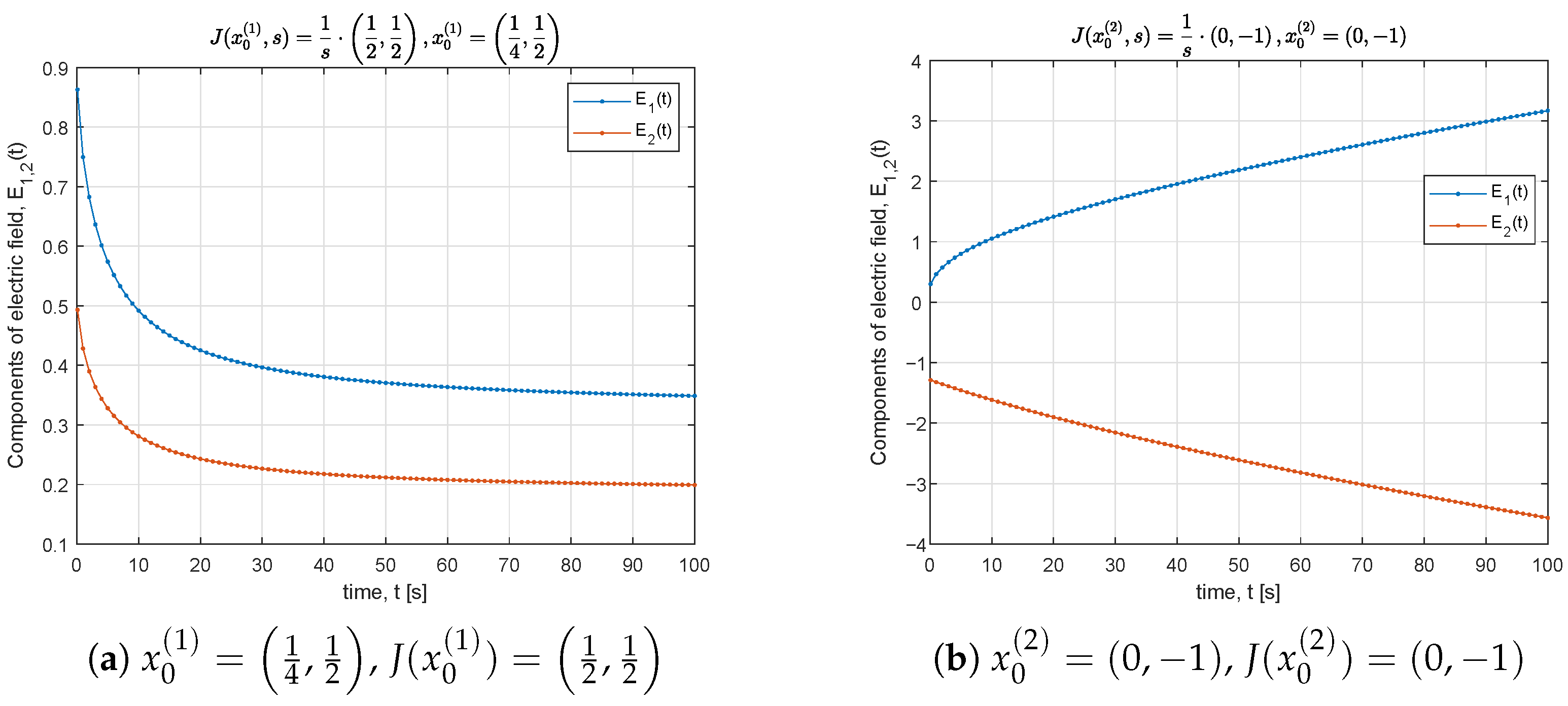
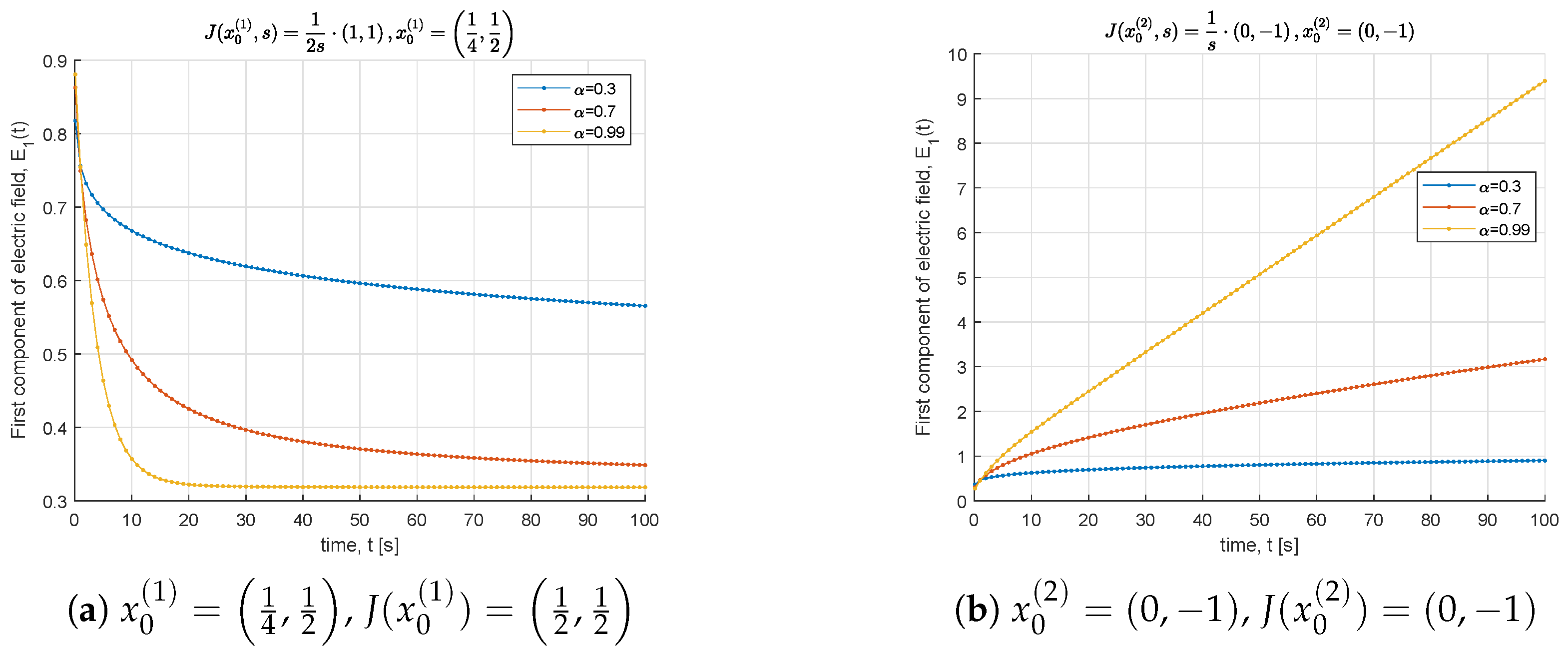
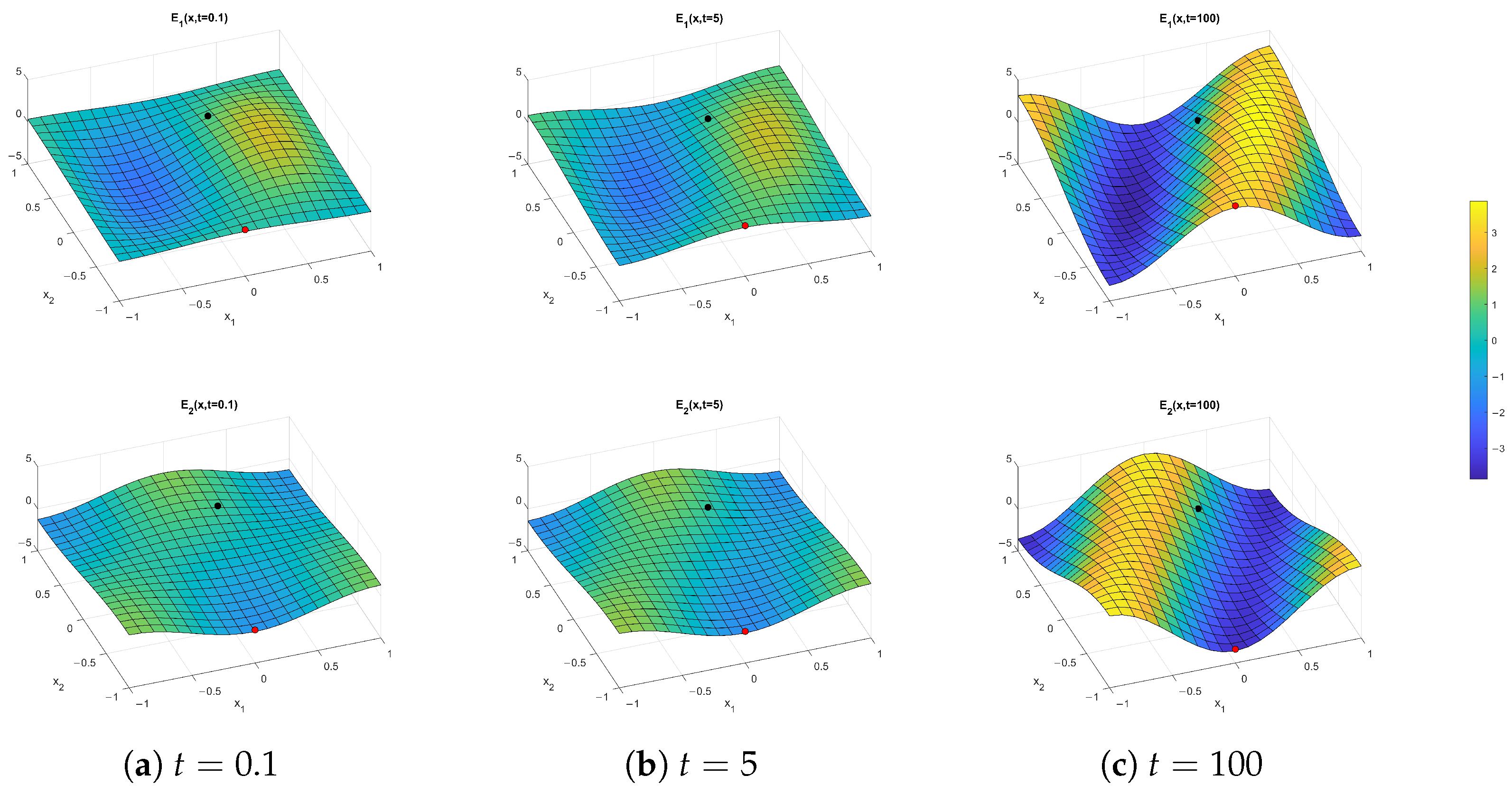
5. Numerical Results

We provide the numerical results that illustrate and confirm our results presented in Proposition 6, proving that the thermodynamic condition (45) is sufficient for the existence of the solution of Equation (50). For illustration purposes, we used MATLAB R2023b environment, which MathWorks, Natick, MA, USA, developed.

In the following example, we determine the distribution of the transverse electric fields $E(x,t)$, $(x_1,x_2)\in \Omega ={[-1,1]}^2$, and $t>0$. It is determined by a given current density $J(x,t)$ through the numeric solution of the inverse Laplace transformation that $E(x,t)={\mathcal{L}}^{-1}\left(E(x,s)\right)\left(t\right)={\mathcal{L}}^{-1}\left(A\left(s\right)J(x,s)\right)\left(t\right)$ and $t>0$, where $A\left(s\right)$ is defined by (54).

We assume that $J(x,t)=J_{sp}\left(x\right)\theta \left(t\right)$, $x\in {[-1,1]}^2$, and $t\in \mathbb{R}$, where

$$\begin{array}{c}\hfill J_{sp}\left(x\right)=\left[\begin{array}{c}sin\left(\pi x_1\right)cos\left({\displaystyle \frac{\pi }{2}}{x}_2\right)\\ cos\left(\pi x_1\right)sin\left({\displaystyle \frac{\pi }{2}}{x}_2\right)\end{array}\right],x\in {[-1,1]}^2\end{array}$$

(56)

and $\theta \left(t\right)$ and $t\in \mathbb{R}$ are the Heaviside functions. Let $\Sigma \left(t\right)={\mathcal{L}}^{-1}\left({\displaystyle \frac{1}{s}}A\left(s\right)\right)\left(t\right)$ and $t>0$. According to previous assumptions,

$$E(x,t)=\Sigma \left(t\right)J_{sp}\left(x\right),x\in {[-1,1]}^2,t>0.$$

To illustrate the time response of the electric field, its components are presented in Figure 1 and Figure 2 at spatial locations of $x_0^{\left(1\right)}=\left({\displaystyle \frac{1}{4}},{\displaystyle \frac{1}{2}}\right)$, where $J_{sp}\left(x_0^{\left(1\right)}\right)=\left({\displaystyle \frac{1}{2}},{\displaystyle \frac{1}{2}}\right)$ and $x_0^{\left(2\right)}=(0,-1)$, where $J_{sp}\left(x_0^{\left(2\right)}\right)=(0,-1)$.

In Figure 1, parameters defining $A\left(s\right)$ are set to the following values: $\alpha =0.7,a=10, b_{11}=5, b_{12}=1, b_{22}=8$, so that sufficient conditions from (45) are satisfied. For the selected parameters in $A\left(s\right)$ and given $J(x,t)$, all the elements are unlimited, i.e., ${\sigma }_{ij}\left(t\right)\to \infty$ and $t\to \infty$. This causes unbounded electric field components with respect to t in the majority of spatial locations, where components of the current density satisfy $J_{sp,1}\left(x_0\right)\ne J_{sp,2}\left(x_0\right)$. This can be easily confirmed analytically by applying the final value theorem ([28], Theorems 34.1 and 33.3), which states

$$\begin{array}{ccc}\hfill & & \underset{t\to \infty }{lim}E(x_0,t)=\underset{s\to 0}{lim}s\widetilde{\Sigma \left(s\right)J_{sp}\left(x_0\right)}=\underset{s\to 0}{lim}A\left(s\right)J_{sp}\left(x_0\right)\hfill \\ & & =\underset{s\to 0}{lim}{\displaystyle \frac{(J_{sp,1}\left(x_0\right)-J_{sp,2}\left(x_0\right))+(J_{sp,1}\left(x_0\right)b_{22}-J_{sp,2}\left(x_0\right)b_{12})s^{\alpha }}{((b_{11}-b_{12})+(b_{22}-b_{12}))s_{\alpha }}}\hfill \end{array}$$

(57)

under some mild conditions on the parameters. Figure 1b illustrates such behavior.

On the contrary, if $J_{sp,1}\left(x_0\right)=J_{sp,2}\left(x_0\right)$, then the components of the electric field will have a horizontal asymptote, which is illustrated in Figure 1a. This follows from (57). Therefore, we conclude that the temporal behavior of $\Sigma \left(t\right)$ will interact with an-isotropic spatial distribution of current $J_{sp}\left(x\right)$, causing a change in the spatial pattern, i.e., redistribution (as time passes) of the local maximum and minimum values of electric field components, which can be seen in Figure 3.

For the presented analysis, the inverse Laplace transform is calculated by a contour integral:

$$f\left(t\right)={\displaystyle \frac{1}{2\pi i}}{\int }_{{\sigma }_0-iW}^{{\sigma }_0+iW}F\left(s\right)e^{st}ds,t>0,$$

where we set ${\sigma }_0=1/100$ and $W=1000$. The numerical results are verified using the Talbot inversion method presented in [29].

6. Conclusions

In the first part of this paper, we present sufficient conditions for the dissipativity property in isothermal conditions for linear, dispersive, anisotropic, and bianisotropic electromagnetic materials in the form of constraints on the parameters of constitutive equations for general fractional distribution-type kernels.

In the second part, those constraints are provided for the particular generalized fractional anisotropic Zener-type model for both the non-homogeneous 3D case and the homogeneous, i.e., 2D, case.

The connection between the restrictions on the parameters of the given fractional Zener-type anisotropic model in the 2D case with the existence and regularity of the solution for the inverse problem of reconstructing the electric field, given the current density for the 2D case in the rectangular domain, is also analyzed.

Some numerical results are also provided to confirm theoretical considerations.

In our future work, we will complete the analysis of the connection of the derived restrictions on the solvability of the system of Maxwell field equations.

References

1. Orfanidis, S.J. Electromagnetic Waves and Antennas. 2016. Available online: https://www.mathworks.com/academia/books/electromagnetic-waves-and-antennas-orfanidis.html (accessed on 7 November 2024).
2. Nunes, F.D.; Vasconcelos, T.C.; Bezerra, M.; Weiner, J. Electromagnetic energy density in dispersive and dissipative media. J. Opt. Soc. Am. B 2011, 28, 1544–1552. [Google Scholar] [CrossRef]
3. Caloz, C.; Itoh, T. Electromagnetic Metamaterials: Transmission Line Theory and Microwave Applications; John Wiley & Sons: Hoboken, NJ, USA, 2005. [Google Scholar] [CrossRef]
4. Jackson, J.D. Classical Electrodynamics, 2nd ed.; John Wiley & Sons: Hoboken, NJ, USA, 1975; Chapter 7. [Google Scholar]
5. Quan, L.; Alù, A. Passive Acoustic Metasurface with Unitary Reflection Based on Nonlocality. Phys. Rev. Appl. 2019, 11, 054077. [Google Scholar] [CrossRef]
6. Kwon, H.; Sounas, D.; Cordaro, A.; Polman, A.; Alù, A. Nonlocal Metasurfaces for Optical Signal Processing. Phys. Rev. Lett. 2018, 121, 173004. [Google Scholar] [CrossRef] [PubMed]
7. Nasrolahpour, H. A note on fractional electrodynamics. Commun. Nonlinear Sci. Numer. Simul. 2013, 18, 2589–2593. [Google Scholar] [CrossRef]
8. Nasrolahpour, H. Fractional electromagnetic metamaterials. Optik 2020, 203, 163969. [Google Scholar] [CrossRef]
9. Karlsson, A.; Kristensson, G. Constitutive Relations, Dissipation, and Reciprocity for the Maxwell Equations in the Time Domain. J. Electromagn. Waves Appl. 1992, 6, 537–551. [Google Scholar] [CrossRef]
10. Coleman, B.; Dill, E. Thermodynamic restrictions on the constitutive equations of electromagnetic theory. Z. Angew. Math. Phys. 1971, 22, 691–702. [Google Scholar] [CrossRef]
11. Coleman, B.D.; Dill, E.H. On the thermodynamics of electromagnetic fields in materials with memory. Arch. Ration. Mech. Anal. 1971, 41, 132–162. [Google Scholar] [CrossRef]
12. Cassier, M.; Joly, P.; Kachanovska, M. Mathematical models for dispersive electromagnetic waves: An overview. Comput. Math. Appl. 2017, 74, 2792–2830. [Google Scholar] [CrossRef]
13. Amendola, G.; Fabrizio, M.; Golden, J.M. A Mathematical Model for Visco-Ferromagnetic Materials. Prog. Fract. Differ. Appl. 2020, 6, 245–252. [Google Scholar] [CrossRef]
14. Cassier, M.; Hazard, C.; Joly, P. Spectral theory for Maxwell’s equations at the interface of a metamaterial. Part I: Generalized Fourier transform. Commun. Partial. Differ. Equ. 2017, 42, 1707–1748. [Google Scholar] [CrossRef]
15. Kovačević, J.; Cvetićanin, S.M.; Zorica, D. Electromagnetic field in a conducting medium modeled by the fractional Ohm’s law. Commun. Nonlinear Sci. Numer. Simul. 2022, 114, 106706. [Google Scholar] [CrossRef]
16. Moreles, M.A.; Lainez, R. Mathematical modelling of fractional order circuit elements and bioimpedance applications. Commun. Nonlinear Sci. Numer. Simul. 2017, 46, 81–88. [Google Scholar] [CrossRef]
17. Truesdell, C. Das ungelöste Hauptproblem der endlichen Elastizitätstheorie. ZAMM Z. Angew. Math. Mech. (J. Appl. Math. Mech.) 1956, 36, 97–103. [Google Scholar] [CrossRef]
18. Fabrizio, M.; Morro, A. Dissipativity and irreversibility of electromagnetic systems. Math. Model. Methods Appl. Sci. 2000, 10, 217–246. [Google Scholar] [CrossRef]
19. Fabrizio, M.; Morro, A. Mathematical Problems in Linear Viscoelasticity; Society for Industrial and Applied Mathematics: Philadelphia PA, USA, 1992. [Google Scholar]
20. Šarčev, I.; Šarčev, B.P.; Krstonošić, V.; Janev, M.; Atanacković, T.M. Modeling the rheological properties of four commercially available composite core build-up materials. Polym. Polym. Compos. 2021, 29, 931–938. [Google Scholar] [CrossRef]
21. Atanacković, T.M.; Janev, M.; Pilipović, S. On the thermodynamical restrictions in isothermal deformations of fractional Burgers model. Philos. Trans. R. Soc. Math. Phys. Eng. Sci. 2020, 378, 20190278. [Google Scholar] [CrossRef] [PubMed]
22. Atanacković, T.M.; Pilipović, S.; Stanković, B.; Zorica, D. Fractional Calculus with Applications in Mechanics: Vibrations and Diffusion Processes; John Wiley & Sons, Inc.: Hoboken, NJ, USA, 2014. [Google Scholar] [CrossRef]
23. Bagley, R.; Torvik, P. On the Fractional Calculus Model of Viscoelastic Behavior. J. Rheol. 1986, 30, 133–155. [Google Scholar] [CrossRef]
24. Schwartz, L. Théorie des Distributions; Hermann: Paris, France, 1966; pp. xiii+420. [Google Scholar]
25. Vladimirov, V.S. Methods of the theory of generalized functions. In Analytical Methods and Special Functions; Taylor & Francis: London, UK, 2002; Volume 6, pp. xiv+311. [Google Scholar]
26. Reed, M.; Simon, B. Methods of Modern Mathematical Physics: Functional Analysis; Number 1 in Methods of Modern Mathematical Physics; Academic Press: Cambridge, MA, USA, 1980. [Google Scholar]
27. Micheli, M.; Glaunes, J. Matrix-valued Kernels for Shape Deformation Analysis. Geom. Imaging Comput. 2013, 1, 57–139. [Google Scholar] [CrossRef]
28. Doetsch, G. Introduction to the Theory and Application of the Laplace Transformation; Springer: Berlin/Heidelberg, Germany, 1974. [Google Scholar] [CrossRef]
29. McClure, T. Numerical Inverse Laplace Transform. MATLAB Central File Exchange. 2013. Available online: https://www.mathworks.com/matlabcentral/fileexchange/39035-numerical-inverse-laplace-transform (accessed on 7 November 2024).
Figure 1. Time response of E 1 ( x 0 , t ) and E 2 ( x 0 , t ) at different spatial locations, x 0 ( 1 ) and x 0 ( 2 ) . The values of parameters defining A ( s ) are α = 0.7 , a = 10 ,   b 11 = 5 ,   b 12 = 1 ,   b 22 = 8 .
Fractalfract 09 00342 g001
Figure 2. Time response of E 1 ( x 0 , t ) at different spatial locations, x 0 ( 1 ) and x 0 ( 2 ) , and for different values of parameters, α { 0.3 , 0.7 , 0.99 } . The values of the remaining parameters defining G 1 ( s ) are a = 10 , b 11 = 5 , b 12 = 1 , b 22 = 8 .
Fractalfract 09 00342 g002
Figure 3. Space–time distribution of E ( x , t ) for x 1 , 2 [ 1 , 1 ] at different times: (a) t = 0.1 , (b) t = 5 , and (c) t = 100 . The values of parameters defining A ( s ) are α = 0.7 , a = 10 ,   b 11 = 5 ,   b 12 = 1 ,   b 22 = 8 , and they correspond to Figure 1. (Black and red markers indicate spatial positions x 0 ( 1 ) and x 0 ( 2 ) , respectively, which are used for temporal analysis in Figure 1 and Figure 2). We have max x [ 1 , 1 ] 2 E ( x , t = 0.1 ) 2 2.05 , max x [ 1 , 1 ] 2 E ( x , t = 5 ) 2 2.11 , and max x [ 1 , 1 ] 2 E ( x , t = 100 ) 2 5 .
Fractalfract 09 00342 g003
Disclaimer/Publisher’s Note: The statements, opinions and data contained in all publications are solely those of the individual author(s) and contributor(s) and not of MDPI and/or the editor(s). MDPI and/or the editor(s) disclaim responsibility for any injury to people or property resulting from any ideas, methods, instructions or products referred to in the content.