Using He’s Two-Scale Fractal Transform to Predict the Dynamic Response of Viscohyperelastic Elastomers with Fractal Damping

Abstract

This article aims to clarify the applicability of He’s two-scale fractal dimension transform by replacing $t^{\mathsf{\alpha }}$ with $\mathsf{\tau }$. It demonstrates the potential to capture the influence of the fractal parameter on the system’s damping frequency, particularly when the viscoelastic term (damping) does not equal half of the fractional inertia force term. The analysis examines the elastomer materials’ dynamic fractal amplitude–time response, considering the viscohyperelastic effects related to the material’s energy dissipation capacity. To determine the amplitude of oscillations for the nonlinear equation of motion of a body supported by a viscohyperelastic elastomer subjected to uniaxial stretching, the harmonic balance perturbation method, combined with the two-scale fractal dimension transform and Ross’s formula, is employed. Numerical calculations demonstrate the effectiveness of He’s two-scale fractal transformation in capturing fractal phenomena associated with the fractional time derivative of deformation. This is due to a correlation between the fractional rate of viscoelasticity and the fractal structure of media in elastomer materials, which is reflected in the oscillation amplitude decay. Furthermore, the approach introduced by El-Dib to replace the original fractional equation of motion with an equivalent linear oscillator with integer derivatives is used to further assess the qualitative and quantitative performance of our derived solution. The proposed approach elucidates the applicability of He’s two-scale fractal calculus for determining the amplitude of oscillations in viscohyperelastic systems, where the fractal derivative order of the inertia and damping terms varies.

1. Introduction

The two-scale dimension transform aids in observing the same phenomena using a large scale, which describes the physical behavior that occurs at the continuous level, and a smaller scale to capture effects that appear at the molecular level and in a discontinuous medium [1,2,3,4]. Previously, the two-scale dimension transform has been used successfully in modeling nonlinear phenomena, such as the instability of the electrospinning process [5]; Fangzhu’s water collector [6]; studying waves traveling along a porous surface [4]; determining the low-frequency property of a concrete beam [7]; modeling fractal oscillators [8,9,10,11]; microgravity oscillators [12]; population dynamics [13]; non-Gaussian polymer chain motion [14]; plasma frequency changes [15]; fractal damping Duffing-jerk oscillator [16]; and porous properties of concrete beams [7], to name a few.

On the other hand, the complexity of solving the fractal differential equation of motion increases when the fractional order derivative of the damping term is not half of the fractional inertia force, something that occurs when modeling the motion of an immersed plate in a Newtonian fluid of finite extent [17], in a viscous body deformation under given stress [18], in sound absorption of acoustic metamaterials with two face-sheets and a swastika fractal structure core [19], in studying the dynamics of thin plates [20], and in the fractal prediction of normal contact damping on mechanical joint surfaces [21]. Of course, differential equations with fractional damping terms also describe additional phenomena in electromagnetics, electrochemistry, and material science, to name a few. Because of the importance of having a good description of the above phenomena, one must derive approximate solutions to these fractal differential equations to predict their qualitative and quantitative behavior, and thus, several approximate solutions have been proposed in the literature for some differential equations with fractal velocity terms [22,23,24,25,26,27]. El-Dib and Elgazery introduced a linearization method to transform the fractal vibration system to the traditional damping vibration theory and concluded that the fractal derivative plays a damping role that cannot be observed if the fractal time $t^{\mathsf{\alpha }}$ is replaced with a new variable $\mathsf{\tau }$ [28]. Here, we introduce an approach that illustrates how the fractal time derivative can be replaced with a new variable that captures and predicts the system’s behavior under study for different fractal dimension values. Our proposed approach enhances the applicability of He’s two-scale fractal dimension transform to study nonlinear phenomena found in polymer materials, such as those related to optical properties, polymer processing, rheology, stress relaxation behavior, and magnetorheological effects, to name a few [29,30]. Recently, multiscale theories have been developed to explain how rheological properties of polymers are connected to their network structure fractal dimension, allowing the depiction of different rheological behaviors when subjected to various temperatures, strain rates, or magnetic fields [31,32]. Furthermore, these theories could be expanded to investigate wave propagation in fractal media, connecting their fractal dimension with their dissipation energy capacity and oscillation amplitudes [33].

Therefore, this article aims to clarify the applicability of He’s two-scale fractal dimension transform by replacing $t^{\mathsf{\alpha }}$ with $\mathsf{\tau }$. It demonstrates the potential to capture the influence of the fractal parameter on the system’s damping frequency, particularly when the viscoelastic term (damping) does not equal half of the fractional inertia force term. The analysis examines the elastomer materials’ dynamic fractal amplitude–time response, considering the viscohyperelastic effects related to energy dissipation capacity. Also, the fractional derivative definition introduced by Ross in [34] is used with the harmonic balance method to derive an approximate solution that provides the expressions needed to connect the fractal parameter value with the energy dissipation material properties. We want to point out that in the available literature, there are other fractional derivative definitions, such as the Caputo, Atangana–Baleanu [35], Caputo-Fabrizio [36], and constant proportional–Caputo hybrid [37], to name a few, but none of these fractional derivative definitions have, to the best of our knowledge, been used with He’s two-scale transform to address the solution of a fractal differential equation of motion with damping terms having fractal exponents that are not half of the inertia term.

Thus, our research focuses on using the fractal derivative definition introduced by Ross [35] to solve the fractal equation of motion that models elastomer dynamics, analyze wave propagation in fractal polymer media, and gain deeper insight into how wave propagation takes place as a function of the inertia and damping fractal dimension values.

Numerical calculations show the effectiveness of He’s two-scale fractal transformation in capturing fractal phenomena associated with the fractional time derivative of deformation since there is a correlation between the fractional rate of viscoelasticity and the fractal structure of media in elastomer materials, which is reflected in modeling its displacements and in the oscillation amplitude decay due to relaxation phenomena linked to an increase in the material entropy caused by internal molecular friction, which produces changes in the material structure that affect the relaxation modes [38,39,40,41,42].

The paper is organized as follows. We begin in Section 1 with a brief review of the applicability of the two-scale dimension transformation to solve problems that deal with multiscale physics processes. Section 2 introduces the derivation of the fractal differential equation that describes the dynamic behavior of viscohyperplastic materials. The equivalent representation form of the conservative force exerted by the material molecular chains is derived in Section 3 using a cubication method that allows writing the fractal equation of motion as an equivalent damped homogeneous Duffing’s expression. The approximate analytical solution of the equivalent fractal equation of motion using the Ross fractional derivative definition and the harmonic balance method is derived in Section 4. Results demonstrating the accuracy attained by our derived solution compared to the exact numerical integration of the original equation of motion are discussed in Section 5. Also, at the end of Section 5, we compare our derived solution with the one derived by replacing the original fractional equation of motion with an equivalent nonlinear oscillator.

2. A Dynamic Viscohyperelastic Model of Elastomer Materials

The fractal Lagrange equation of the form:

$${\displaystyle \frac{d}{d{t}^{\mathsf{\alpha }}}}\left({\displaystyle \frac{\partial L}{\partial \dot{q_i}}}\right)-{\displaystyle \frac{\partial L}{\partial q_i}}=Q_i,$$

(1)

can be used to derive the equation of motion of viscohyperelastic elastomer materials [14]. In Equation (1), $L=T-V$ is the Lagrangian, $T$ is the kinetic energy, $V$ is the Langevin material potential energy, $Q_i$ are non-conservative generalized forces, and the overdot denotes derivative with respect to time [43,44,45,46]. According to [14], the mathematical expressions to determine $L$ and $V$ are given by:

$$T={\displaystyle \frac{1}{2}}M{\left({\displaystyle \frac{d{q}_i}{d{t}^{\mathsf{\alpha }}}}\right)}^2,$$

(2)

$$V=kNT{\int }_0^{{\displaystyle \frac{x}{L_1}}}{\mathcal{L}}^{-1}\left(q_i\right)d{q}_i$$

(3)

where $M$ is the body mass, $t$ is the current time, $\alpha$ is the fractal dimension of the inertia terms, $q_i$ are the generalized coordinates representing material strains, $Q_i$ are the generalized system driving forces and dissipative ones, $k$ is Boltzmann constant, $T$ is the absolute temperature, $N$ is the chain number of rigid links, and ${\mathcal{L}}^{-1}\left(q_i\right)$ is the inverse of the Langevin chain function, defined as:

$$q_i=\mathcal{L}\left({\beta }_0\right)=\coth {\beta }_0-{\displaystyle \frac{1}{{\beta }_0}}.$$

(4)

If we assume that the chain is subjected to the action of dissipation phenomena due to relaxation, frictional stick–slip, and restoration of the polymer chain network effects, then the governing equation of motion of a body of mass $M$ supported by a viscohyperelastic elastomer material becomes:

$$L_{1}M{\displaystyle \frac{d}{d{t}^{\alpha }}}\left({\displaystyle \frac{d}{d{t}^{\alpha }}}\right)+{\nu }_0{\displaystyle \frac{dy}{d{t}^{\alpha }}}+\left(kNT\right){\mathcal{L}}^{-1}\left(y\right)=0,y\left(0\right)=A,{\displaystyle \frac{dy}{d{t}^{\alpha }}}=V_0$$

(5)

where ${\mathsf{\nu }}_0$ is a damping constant, ${\mathsf{\alpha }}_1$ is the fractal dimension associated with the polymer network configurational losses [41,47] and its crosslink density [42], $L_1$ represents the undeformed chain length, and $A$ and $V_0$ are the initial stretch and velocity experienced by the polymer chains.

Using He two-scale dimension transform [28,48,49,50]:

$$\tau =t^{\alpha }$$

(6)

and the fractal derivative definition:

$${\displaystyle \frac{dy}{d{t}^{\alpha }}}\left(t_0^{\alpha }\right)=\mathsf{\Gamma }\left(1+\alpha \right)\underset{{\displaystyle \frac{\left(t-t_0\right)\to \Delta t}{\Delta t\ne 0}}}{\lim }{\displaystyle \frac{y\left(t\right)-y\left(t_0\right)}{{\left(t-t_0\right)}^{\alpha }}}$$

(7)

Equation (5) can be written as:

$$L_{1}M{\displaystyle \frac{d^{2}y}{d{\tau }^2}}+{\nu }_0{\displaystyle \frac{dy}{d{\tau }^{\gamma }}}+\left(kNT\right){\mathcal{L}}^{-1}\left(y\right)=0,y\left(0\right)=A,{\displaystyle \frac{d}{d{t}^{1/\alpha }}}y(0)=V_0$$

(8)

with $\mathsf{\gamma }={\mathsf{\alpha }}_1/\alpha$. The close-form solution of Equation (8) is unknown because of the complexity associated with the inverse of the Langevin function ${\mathcal{L}}^{-1}\left(y\right)$; therefore, we use its approximate form proposed in [44,46], given as:

$${\mathcal{L}}^{-1}\left(y\right)\cong {\displaystyle \frac{y\left(30-26y+7y^2\right)}{3\left(1-ay\right)\left(10+ay\right)}}$$

(9)

hence, Equation (8) becomes:

$${ML}_1{\displaystyle \frac{d^{2}y}{d{\tau }^2}}+{\nu }_0{\displaystyle \frac{dy}{d{\tau }^{\gamma }}}+{\displaystyle \frac{\left(kNT\right)}{3}}{\displaystyle \frac{ay\left(30-26ay+7a^2{y}^2\right)}{\left(1-ay\right)\left(10+ay\right)}}=0$$

(10)

where $a=1/y_0$, and $y_0$ represents the maximum possible polymer chain strain value. Notice from Equation (10) that the irrational polynomial representation form of the conservative restoring force introduces a higher degree of complexity to derive approximate analytical solutions using perturbation methods such as averaging, harmonic balance, multiple scales, and homotopy, to name a few. Therefore, in the next section, we shall derive the equivalent polynomial representation form of (8) by applying the enhanced cubication method.

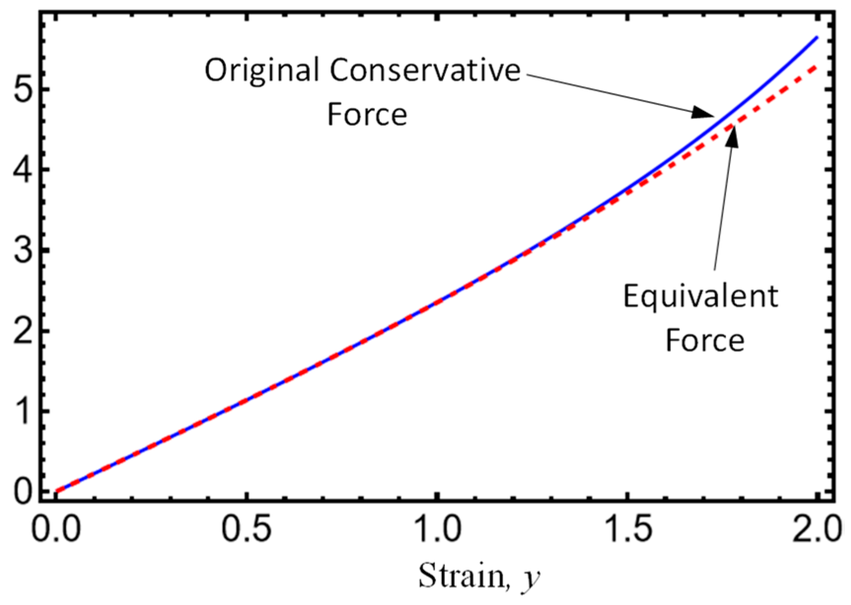
Equivalent Conservative Restoring Force

The equivalent representation form of the conservative restoring force of Equation (10) is derived using the enhanced cubication method proposed in [51]. In this methodology, the conservative restoring force is replaced by an equivalent cubic polynomial expression using the equation:

$$U={\int }_0^{\sigma }{\left[{\displaystyle \frac{\left(kNT\right)}{3}}{\displaystyle \frac{ay\left(30-26ay+7a^2{y}^2\right)}{\left(1-ay\right)\left(10+ay\right)}}-a_{1}y-a_2{y}^3\right]}^{2}w\left(y\right)dy$$

(11)

where the weighted function $w\left(y\right)$ takes the form $w\left(y\right)=y^{N_1}$ to ensure that the equivalent restoring force $a_{1}y+a_2{y}^3$ reproduces the original one’s quantitative and qualitative behaviors as discussed in [52,53,54,55,56]. Following the enhanced cubication method discussed in [51], the expressions

$${\displaystyle \frac{\partial U}{\partial a_1}}=0,{\displaystyle \frac{\partial U}{\partial a_2}}=0$$

(12)

allow the determination of the parameters $a_1$, $a_2$, and $N_1$ that minimize the weighted mean square error $U$. We recall that in this methodology, one can assume that the dissipating force term is the same in the original and equivalent equations of motion. Using Equations (11) and (12) yields the expressions for $a_1$ and $a_2$:

$$\begin{array}{l}{a}_1=kNT/(12a^3\left(1+N_1\right)\left(2+N_1\right)\left(4+N_1\right){\sigma }^4)(90001\left(2+N_1\right)\left(3+N_1\right)\left(4+N_1\right)\left(5+N_1\right)\left(7+N_1\right)\\ -8999a\left(1+N_1\right)\left(3+N_1\right)\left(4+N_1\right)\left(5+N_1\right)\left(7+N_1\right)y-7208a^2\left(2+N_1\right)\left(4+N_1\right)\left(5+N_1\right){\sigma }^2\\ +534a^3\left(1+N_1\right)\left(3+N_1\right)\left(5+N_1\right){\sigma }^3-28a^4\left(1+N_1\right)\left(2+N_1\right)\left(4+N_1\right){\sigma }^4\\ +\mathsf{\Gamma }[6+N_1](900\left(-100\left(7+N_1\right)+a^2\left(5+N_1\right){\sigma }^2\right){}_{2}F_1\left[1,1+N_1,2+N_1,-ay/10\right]\\ +\left(a^2\left(5+N_1\right){\sigma }^2-7-N_1\right){}_{2}F_1\left[1,1+N_1,2+N_1,-ay\right]))\end{array}$$

(13)

$$\begin{array}{l}{a}_2=kNT/(12{\sigma }^6)\left(5+N_1\right)\left(7+N_1\right)(-((90001\left(5+N_1\right))/(a^3\left(1+N_1\right)))\\ +8999\left(5+N_1\right)\sigma )/(a^2\left(2+N_1\right)+3604{\sigma }^2/(a(3+4N_1+N_1^2))-178{\sigma }^3/(8+6N_1+N_1^2)\\ +1/(a^3\left(1+N_1\right))(-900(-100\left(5+N_1\right)+a^2\left(3+N_1\right){\sigma }^2){}_{2}F_1\left[1,1+N_1,2+N_1,-{\displaystyle \frac{a\sigma }{10}}\right]\\ +\left(5+N_1-a^2\left(3+N_1\right){\sigma }^2){}_{2}F_1\left[1,1+N_1,2+N_1,-a\sigma \right]\right))\end{array}$$

(14)

where ${}_{2}F_1$, ${}_2\overline{F_1}$, and $\mathsf{\Gamma }$ are, respectively, the hypergeometric, regularized hypergeometric, and Gamma functions. As usual, the value of $\mathsf{\sigma }$ is fit to minimize the error of replacing the original restoring force by an equivalent one [51]. Thus, the equivalent representation form of Equation (10) becomes:

$$M{L}_1{\displaystyle \frac{d^{2}y}{d{\tau }^2}}+{\nu }_0{\displaystyle \frac{dy}{d{\tau }^{\gamma }}}+\left(kNT\right)a_{1}y+\left(kNT\right)a_2{y}^3=0$$

(15)

which can be rewritten as:

$${\displaystyle \frac{d^{2}y}{d{\tau }^2}}+2\nu {\omega }_n{\displaystyle \frac{dy}{d{\tau }^{\gamma }}}+{\omega }_n^{2}y+\epsilon y^3=0,y\left(0\right)=y_0,{\displaystyle \frac{d}{d{\tau }^{\gamma }}}y\left(0\right)=V_0$$

(16)

with:

$$2\nu {\omega }_n\equiv {\displaystyle \frac{{\nu }_0}{M{L}_1}},{\omega }_n^2\equiv {\displaystyle \frac{a_1\left(kNT\right)}{M{L}_1}},\epsilon \equiv {\displaystyle \frac{\left(kNT\right)a_2}{M{L}_1}}$$

(17)

One must notice that when $\alpha =1$ and $\gamma =1$, Equation (16) becomes the traditional damped, homogeneous Duffing’s equation. Because of the nature of the dynamic system in general, $\mathsf{\gamma }\ne 1,$ and then the solution of Equation (16) cannot be obtained in closed form.

3. Approximate Solution

To find an approximate solution for the fractal system (16), we follow a new solution approach that considers the fractional derivative definition introduced by Ross in [34]:

$${\displaystyle \frac{dy}{d{\mathsf{\tau }}^{\mathsf{\gamma }}}}={\displaystyle \frac{1}{\mathsf{\Gamma }\left(1-\mathsf{\gamma }\right)}}\left({\int }_0^{\mathsf{\tau }}{v}^{-\mathsf{\gamma }}{y}^{\prime }\left(\mathsf{\tau }-v\right)dv+{\displaystyle \frac{y\left(0\right)}{{\mathsf{\tau }}^{\mathsf{\gamma }}}}\right),$$

(18)

and assume that $y\left(0\right)=0$; then, Equation (18) reduces to:

$${\displaystyle \frac{dy}{d{\tau }^{\gamma }}}={\displaystyle \frac{1}{\Gamma \left(1-\gamma \right)}}{\int }_0^{\tau }{v}^{-\gamma }{y}^{\prime }\left(\tau -v\right)dv$$

(19)

In order to obtain an approximate solution for Equation(16), we assume that:

$$y\left(\tau \right)=e^{-n_1\nu {\omega }_n\tau }\left(A\cos \left({\omega }_d\tau \right)+B\sin \left({\omega }_d\tau \right)\right)$$

(20)

where $n_1$ and ${\omega }_d$ are assumed to be slowly varying as a function of time such that their derivatives with respect to time become zero. $A$ and $B$ are constants that could be determined using the system’s initial conditions: $y\left(0\right)=0$, $dy\left(0\right)/d{\mathsf{\tau }}^{\mathsf{\gamma }}=V_0$. These yield:

$$A=0,\hspace{1em}B=V_0/{\mathsf{\omega }}_d$$

(21)

The substitution of Equations (19) and (21) into Equation (16) yields the expression needed to compute the parameters $n_1$, and ${\mathsf{\omega }}_d$:

$$\begin{array}{l}{B}^3{\mathsf{\tau }}^{\mathsf{\gamma }}\mathsf{\epsilon }\mathsf{\Gamma }\left[1-\mathsf{\gamma }\right]{\sin }^3\left(\mathsf{\tau }{\mathsf{\omega }}_d\right)+{\displaystyle \frac{1}{2}}B{e}^{2n_1\mathsf{\tau }\mathsf{\nu }{\mathsf{\omega }}_n-i\mathsf{\tau }{\mathsf{\omega }}_d}\\ (-2e^{2i\mathsf{\tau }{\mathsf{\omega }}_d}\mathsf{\tau }\mathsf{\nu }E\left[\mathsf{\gamma },i\mathsf{\tau }{\mathsf{\omega }}_d-n_1\mathsf{\tau }\mathsf{\nu }{\mathsf{\omega }}_n\right]{\mathsf{\omega }}_n\left({\mathsf{\omega }}_d+i{n}_1\mathsf{\nu }{\mathsf{\omega }}_n\right)+2i\mathsf{\tau }\mathsf{\nu }E\left[\mathsf{\gamma },-i\mathsf{\tau }{\mathsf{\omega }}_d-n_1\mathsf{\tau }\mathsf{\nu }{\mathsf{\omega }}_n\right]{\mathsf{\omega }}_n\left(i{\mathsf{\omega }}_d+n_1\mathsf{\nu }{\mathsf{\omega }}_n\right)\\ +{\mathsf{\tau }}^{\mathsf{\gamma }}\mathsf{\Gamma }\left[1-\mathsf{\gamma }\right](i\left(e^{2i\mathsf{\tau }{\mathsf{\omega }}_d}-1\right){\mathsf{\omega }}_d^2-2\left(1+e^{2i\mathsf{\tau }{\mathsf{\omega }}_d}\right)n_1\mathsf{\nu }{\mathsf{\omega }}_d{\mathsf{\omega }}_n\\ +2{\mathsf{\omega }}_n\left(e^{i\mathsf{\tau }{\mathsf{\omega }}_d}\left(1+n_1^2{\mathsf{\nu }}^2\right)\sin \left(\mathsf{\tau }{\mathsf{\omega }}_d\right){\mathsf{\omega }}_n+i\mathsf{\nu }\left({\left(-i{\mathsf{\omega }}_d-n_1\mathsf{\nu }{\mathsf{\omega }}_n\right)}^{\mathsf{\gamma }}-e^{2i\mathsf{\tau }{\mathsf{\omega }}_d}{\left(i{\mathsf{\omega }}_d-n_1\mathsf{\nu }{\mathsf{\omega }}_n\right)}^{\mathsf{\gamma }}\right)\right)\left)\right)=0\end{array}$$

(22)

where $E\left[\gamma ,-i\tau {\omega }_d-n_1\tau \nu {\omega }_n\right]$ is the exponential integral function defined as ${\int }_1^{\infty }{\tau }^{-\tau \left(i{\omega }_d-n_1\nu {\omega }_n\right)}{e}^{-\gamma \tau }d\tau$ with $\left(\gamma \ge 0\right)$, $\Gamma$ is the Gamma function, $i=\sqrt{-1}$, and $\mathsf{\tau }$ is assumed to be equal to the elapsed time to reach the maximum system oscillation displacement, i.e., $\tau =1/4\pi /{\omega }_d$. Following the harmonic balance procedure, we obtain, from Equation (22), the following expressions:

$$\begin{array}{l}\mathit{cos}\left({\omega }_d\tau \right)\cdot 4iB\nu {\omega }_n{e}^{2n_1\tau \nu {\omega }_n}\\ (i\tau E\left[\gamma ,i\tau {\omega }_d-n_1\tau \nu {\omega }_n\right]\left({\omega }_d+i{n}_1\nu {\omega }_n\right)+\tau E\left[\gamma ,-i\tau {\omega }_d-n_1\tau \nu {\omega }_n\right]\left(i{\omega }_d+n_1\nu {\omega }_n\right)\\ +{\tau }^{\gamma }\Gamma \left[1-\gamma \right]\left(2i{n}_1{\omega }_d+{\left(-i{\omega }_d-n_1\nu {\omega }_n\right)}^{\gamma }-{\left(i{\omega }_d-n_1\nu {\omega }_n\right)}^{\gamma }\right))\\ +\mathit{sin}\left({\omega }_d\tau \right)\cdot (3B^3{\tau }^{\gamma }\epsilon \Gamma \left[1-\gamma \right]+4B{e}^{2n_1\tau \nu {\omega }_n}(\tau \nu E\left[\gamma ,i\tau {\omega }_d-n_1\tau \nu {\omega }_n\right]{\omega }_n\left(n_1\nu {\omega }_n-i{\omega }_d\right)\\ +\tau \nu E\left[\gamma ,-i\tau {\omega }_d-n_1\tau \nu {\omega }_n\right]{\omega }_n\left(i{\omega }_d+n_1\nu {\omega }_n\right)+{\tau }^{\gamma }\Gamma \left[1-\gamma \right]\\ \left(-{\omega }_d^2+{\omega }_n\left(\left(1+n_1^2{\nu }^2\right){\omega }_n+\nu \left({\left(-i{\omega }_d-n_1\nu {\omega }_n\right)}^{\gamma }+{\left(i{\omega }_d-n_1\nu {\omega }_n\right)}^{\gamma }\right)\right)\right)\left)\right)\\ +\mathit{higher}\mathit{order}\mathit{terms}=0\end{array}$$

(23)

In our solution procedure, the higher-order frequency terms in Equation (23) are neglected, i.e., not considered for determining the parameters $n_1$ and ${\mathsf{\omega }}_d$ [57]. Thus, Equation (23) holds for all time $t$ if and only if:

$$\begin{array}{l}E\left[\gamma ,i\tau {\omega }_d-n_1\tau \nu {\omega }_n\right]\left(i{\omega }_d-n_1\nu {\omega }_n\right)+E\left[\gamma ,-i\tau {\omega }_d-n_1\tau \nu {\omega }_n\right]\left(i{\omega }_d+n_1\nu {\omega }_n\right)\\ +{\tau }^{\gamma -1}\Gamma \left[1-\gamma \right]\left(2i{n}_1{\omega }_d+{\left(-i{\omega }_d-n_1\nu {\omega }_n\right)}^{\gamma }-{\left(i{\omega }_d-n_1\nu {\omega }_n\right)}^{\gamma }\right)=0\end{array}$$

(24)

$$\begin{array}{l}3B^2{\mathsf{\tau }}^{\mathsf{\gamma }-1}\mathsf{\epsilon }\mathsf{\Gamma }\left[1-\mathsf{\gamma }\right]+4e^{2n_1\mathsf{\tau }\mathsf{\nu }{\mathsf{\omega }}_n}(\mathsf{\nu }E\left[\mathsf{\gamma },i\mathsf{\tau }{\mathsf{\omega }}_d-n_1\mathsf{\tau }\mathsf{\nu }{\mathsf{\omega }}_n\right]{\mathsf{\omega }}_n\left(n_1\mathsf{\nu }{\mathsf{\omega }}_n-i{\mathsf{\omega }}_d\right)\\ +\mathsf{\nu }E\left[\mathsf{\gamma },-i\mathsf{\tau }{\mathsf{\omega }}_d-n_1\mathsf{\tau }\mathsf{\nu }{\mathsf{\omega }}_n\right]{\mathsf{\omega }}_n\left(i{\mathsf{\omega }}_d+n_1\mathsf{\nu }{\mathsf{\omega }}_n\right)+{\mathsf{\tau }}^{\mathsf{\gamma }-1}\mathsf{\Gamma }\left[1-\mathsf{\gamma }\right]\\ \left(-{\mathsf{\omega }}_d^2+{\mathsf{\omega }}_n\left(\left(1+n_1^2{\mathsf{\nu }}^2\right){\mathsf{\omega }}_n+\mathsf{\nu }\left({\left(-i{\mathsf{\omega }}_d-n_1\mathsf{\nu }{\mathsf{\omega }}_n\right)}^{\mathsf{\gamma }}+{\left(i{\mathsf{\omega }}_d-n_1\mathsf{\nu }{\mathsf{\omega }}_n\right)}^{\mathsf{\gamma }}\right)\right)\right))=0\end{array}$$

(25)

To determine the unknown parameters $n_1$ and ${\mathsf{\omega }}_d$, Equations (24) and (25) are solved numerically by using the system parameters values of $\mathsf{\nu }$, $\mathsf{\epsilon }$, and $\mathsf{\gamma }$.

4. Results

The assessment of the accuracy attained by our developed solutions was conducted by first considering the equivalent representation form of the conservative restoring force, and second, investigating the accuracy achieved by comparing the approximate solution given by Equation (20) with the numerical integration solution of Equation (16).

4.1. Equivalent Representation Form

Figure 1 illustrates the original restoring force $kNTay\left(30-26ay+7a^2{y}^2\right)/\left(3\left(1-ay\right)\left(10+ay\right)\right)$ plotted with a solid color blue line and its equivalent representation form $kNT\left(a_{1}y+a_2{y}^3\right)$, plotted with a dashed red line, for the parameter values of $M{L}_1=1,$ $kNT=8.0822$, $a=0.2779$, $a_1=0.2783$, and $a_2=0.01237$. Notice that at higher $y$-strain values, the difference between the original and equivalent forces becomes apparent. This confirms that the equivalent transformation approach provides a good estimate of the original restoring force.

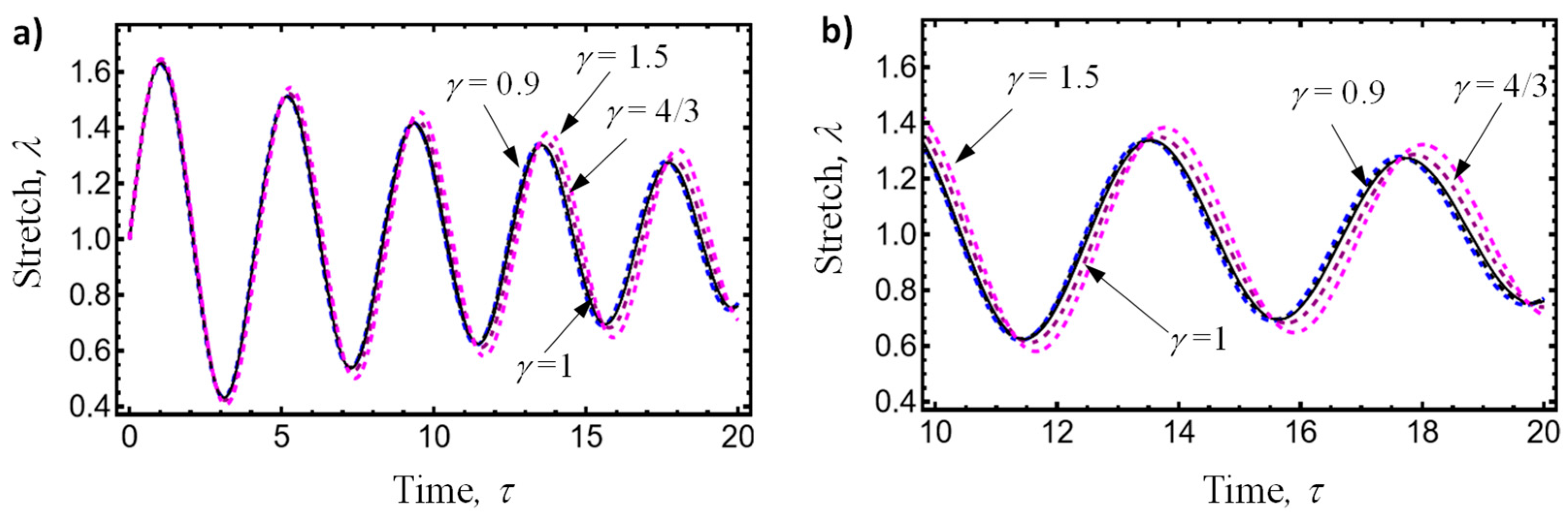
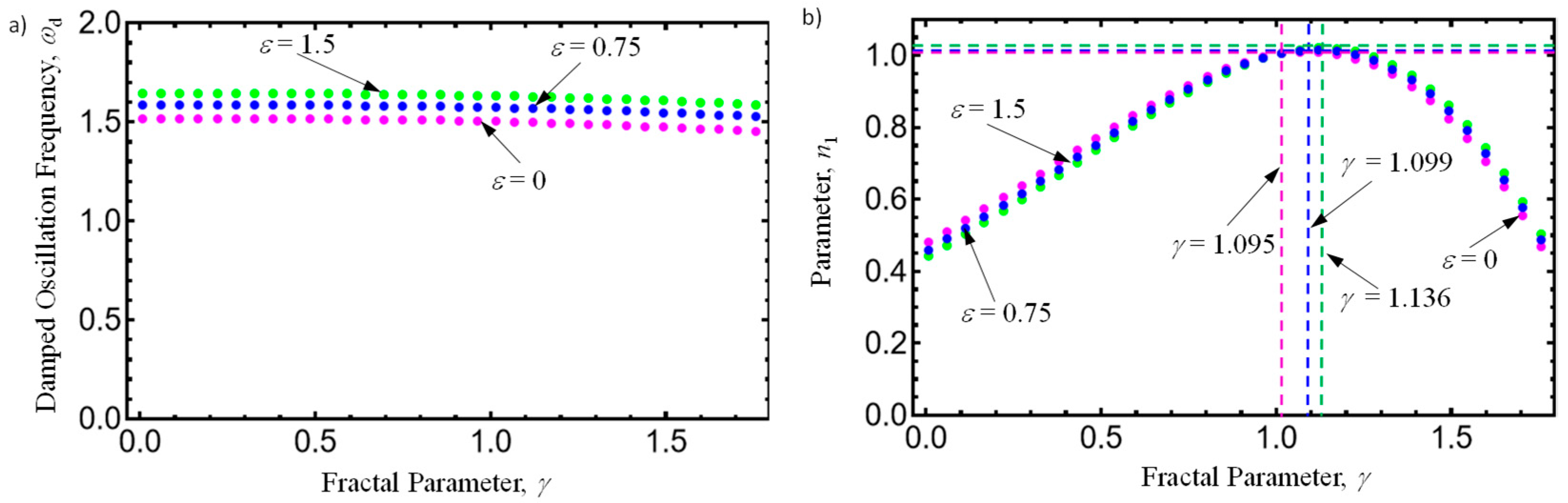
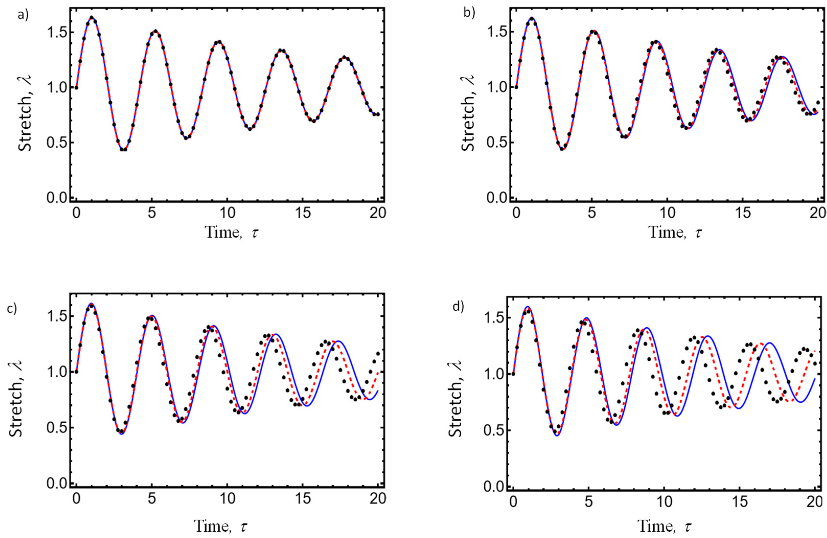
4.2. Numerical Comparison

To investigate the accuracy attained from our proposed derived solution (20) when compared to the numerical integration solution of Equation (16), we consider the following system parameter values: ${\mathsf{\omega }}_n=1.5$, $\mathsf{\nu }=0.0333$, $\mathsf{\epsilon }=0$ with $\mathsf{\alpha }=1$, and $\mathsf{\gamma }=3/4$, $1$, and $4/3$. The numerical exact solution obtained from Equation (16) (solid lines) and the approximate solution given by Equation (20) (dashed lines) are shown in Figure 2a,b, considering that the molecular chain stretch is given as $\mathsf{\lambda }=1+y$, with $\mathsf{\lambda }\left(0\right)=1$ and $\dot{\mathsf{\lambda }}\left(0\right)=\dot{y}\left(0\right)$, and that $\mathsf{\lambda }\ge 1$ when the material is subjected to uniaxial tensile stretching. During the calculation of the approximate amplitude–time response curves using Equation (20), we assumed that $\mathsf{\tau }=\mathsf{\pi }/\left(4{\mathsf{\omega }}_d\right)$ since at this time, the amplitudes of oscillations reach their maximum values during the system’s motion. Notice that in both panels of Figure 2, the fractal stretch–time response curves shift to the left and to the right from the curve obtained for $\mathsf{\gamma }=1$. Furthermore, for fractal parameter values of $\mathsf{\gamma }$ lower than one, it is found that the oscillations’ stretch amplitudes decrease faster with time, and the wavelengths become smaller. This provides information on how the porous medium affects the propagation of waves through it. For instance, when $\mathsf{\gamma }>1$, the waves shift to the right of the curve obtained, with gamma equal to 1, indicating that its propagation speed through the porous viscoelastic medium is higher, as illustrated in Figure 2b. We also observe a difference in the amplitude of the oscillations of the wave. Figure 2 shows that for $\mathsf{\gamma }<1$, the oscillation attenuation in the viscoelastic material increases. This confirms the relationship between the material dissipation energy capacity and its fractal nature. To address the accuracy of our approximate solution, we compute the root-mean-square error value (RMSE). For the parameter values used to perform the simulations, the RMSE value does not exceed $0.045$, which indicates that our approximate solution follows numerical integration well.

As a second example, let us consider the system parameter values of ${\mathsf{\omega }}_n=1.5$ and $\mathsf{\nu }=0.0333$ with $\mathsf{\alpha }=1$, and $\mathsf{\gamma }=0.9$, 1, 4/3, and 1.5. The comparison between our derived solution (20) (dashed line) and the numerical exact integration solution of Equation (16) (solid line) is possible for the values of $\mathsf{\alpha }=1$ and $\mathsf{\gamma }=1$. Figure 3a,b show that both solutions agree well since the maximum RMSE value does not exceed 0.01 for the considered time interval. Once again, the oscillation stretch amplitude decreases faster with time as the fractal parameter value of $\mathsf{\gamma }$ decreases, which indicates the influence that the fractality (porosity) of media has on the decaying effects experienced by the oscillation amplitudes. In Figure 3a,b, the values of $n_1$ and ${\mathsf{\omega }}_d$ of (0.9745,1.513), (1,1.5095), (0.9479,1.4923), and (0.82,1.4805) were obtained by solving Equations (24) and (25) for $\mathsf{\gamma }=0.9$, 1, 4/3, and 1.5, respectively.

Figure 4a,b show the plots of $\mathsf{\gamma }$ vs. ${\mathsf{\omega }}_d$ and $n_1$ vs. ${\mathsf{\omega }}_d$ as a function of the nonlinear parameter $\mathsf{\epsilon }$. Notice that the damped oscillation frequency decreases for increasing values of $\mathsf{\gamma }$, and thus, the wavelengths become smaller, as illustrated in Figure 2 and Figure 3. Notice from Figure 4a that the damped oscillation frequency ${\mathsf{\omega }}_d$ decreases for increasing values of $\mathsf{\gamma }$, and thus, the wavelengths become smaller, as confirmed in Figure 2 and Figure 3. It is also observed in Figure 4b that the maximum values of $n_1$ are reached to the right of the line $\mathsf{\gamma }=$1 and then start to decrease while the system wavelengths rise due to the decreasing values of ${\mathsf{\omega }}_d$, as shown in Figure 4a.

Finally, to show the ability of our solution to provide approximate solutions for the fractal-damped, homogeneous Duffing’s Equation (16), we use the solution for fractional nonlinear oscillators derived by El-Dib in [26]. In that article, El-Dib introduced a novel and elegant approach that facilitates the derivation of analytical solutions of nonlinear oscillators having fractional-order derivatives. El-Dib’s approach is based on replacing the original fractional Equation (16) with an equivalent linear oscillator with integer derivatives whose analytical solution is given as:

$$y\left(\tau \right)=A{e}^{-1/2\mu a_{eq}\tau }\mathit{sin}\Omega \tau ,$$

(26)

with:

$$a_{eq}={\Omega }^{\left(\gamma -1\right)}\mathit{sin}\left({\displaystyle \frac{1}{2}}\pi \gamma \right)$$

(27)

and:

$${\Omega }^2=\left({\omega }_n^2+{\displaystyle \frac{3}{4}}\epsilon A\right)+\mu {\Omega }^{\gamma }\mathit{cos}\left({\displaystyle \frac{1}{2}}\pi \gamma \right)-{\displaystyle \frac{1}{4}}{\mu }^2{\Omega }^{2\left(\gamma -1\right)}{\mathit{sin}}^2\left({\displaystyle \frac{1}{2}}\pi \gamma \right)$$

(28)

where $A$ is the amplitude of oscillations, and $\mu =2\nu {\omega }_n$. Figure 5 shows our derived solution (20) (red dashed line) and the El-Dib solution (26) (black dots) compared to the numerical integration solution of Equation (16) (blue solid line) for the parameter values of ${\mathsf{\omega }}_n=1.5$, $\mathsf{\nu }=0.0333$, $\mathsf{\gamma }=1$, and $\mathsf{\epsilon }=0$, 0.25, 0.75, and 1.5. Notice that for increasing values of $\mathsf{\epsilon }$, both approximate solutions tend to underestimate the numerically exact solution. The error becomes more evident in the El-Dib solution because of the nature of the process followed to derive Equations (26)–(28), which considers using an equivalent linear oscillator to solve Equation (16). In the case of solution (16), its accuracy can be improved if elliptic functions are used instead of trigonometric ones, as discussed in [58]; however, in spite of the limitations exhibited by both approximate solutions, these tend to capture the qualitative and quantitative fractal phenomena exhibited by our viscohyperplastic oscillator, as shown in Figure 6a,b.

Figure 7a,b validate the fractal time transformation of τ = t^α since solutions (20) and (28) capture and predict the system’s behavior for the fractal dimension values shown in both figures. Furthermore, these figures illustrate the role of fractal damping in the system response, even though the fractal time t^α has been replaced with the new variable τ. Figure 7c illustrates the amplitude–time curves when the system damping is almost negligible. Notice that for the time interval shown, the approximate solution curves plotted using the El-Dib approach and our developed solution do not decrease over time due to the small damping value of ν = 0.00001. These solutions agree with the behavior of vibration systems that do not have dissipation energy and with viscohyperplastic materials whose dissipated energy asymptotically decreases to zero when subjected to stress–strain cycling conditions [59]. They also help clarify some misinterpretation in the response of fractional systems, in which the derived solutions lead to an attenuation in the amplitude of oscillations over time, mainly due to decay behavior related to the Mittag–Leffler function [60]. Therefore, we can conclude that He’s two-scale fractal transformation captures the physics of the system well.

5. Conclusions

This article elucidates the applicability of He’s two-scale fractal dimension transform by replacing $t^{\mathsf{\alpha }}$ with τ for finding the approximate fractal amplitude–time responses of the damped Duffing’s equation when the fractional order derivative of the damping term is not half of the fractional inertia force term.

Simulation results demonstrate the applicability of He’s two-scale fractal dimension transform, where $t^{\mathsf{\alpha }}$ is replaced with τ, solving fractal differential equations when the damping term does not equal half of the fractional inertia force term. The approximate solution of the fractal differential equation, which provides the expressions needed to connect the fractal parameter value with the energy dissipation material properties, was derived, replacing the system’s original conservative restoring force with an equivalent cubic polynomial, using Ross’s fractional derivative definition in conjunction with the harmonic balance method.

Furthermore, numerical calculations computed from our proposed solution exhibit higher accuracy than those obtained from the El-Dib approach, as it closely follows the numerical integration solution. Also, we observed that the amplitude–time curves shift to the left ($\mathsf{\gamma }<1$) and to the right ($\mathsf{\gamma }>1$) from the curves obtained for $\mathsf{\gamma }=1$. This implies that when the fractal order of the damping term increases, damping effects are enhanced, and thus, there is a faster decay in the oscillation amplitudes. In other words, for fractal parameter values of γ larger than one, there is a quicker decrease with time of the amplitude of the oscillations.

For increasing values of the nonlinear parameter ε, both approximate solutions tend to underestimate the numerically exact solution. However, the El-Dib solution exhibits the greatest difference when compared to the numerical integration solution, mainly due to the replacement of Equation (16) by an equivalent linear oscillator. In spite of the limitations exhibited by both approximate solutions, their numerical predictions capture the qualitative and quantitative fractal phenomena exhibited by the original fractal oscillator.

It was also observed that both solutions agree well with the behavior of vibration systems without dissipative sources and help to clarify some misinterpretations in the response of fractional systems due to decay behavior related to the Mittag–Leffler functions that are used, in most of the literature, to solve fractional derivative equations.

In summary, our derived solution of Equation (16) could be improved, especially for materials having strong nonlinear behavior, if, for instance, Jacobi elliptic functions were used in Equation (20) to obtain its approximate solution. Needless to say, El-Dib’s approach provides an easy-to-follow solution that could reach a high degree of accuracy if the viscohyperelastic material exhibits weak nonlinear behavior; therefore, his solution can help provide insight into the influence that fractal media have on the dynamic response of the material.

Finally, numerical calculations show the effectiveness of He’s two-scale fractal transformation in capturing the influence of the fractal parameter on the system’s damping frequency, allowing the examination of elastomer materials’ dynamic fractal amplitude–time decay due to relaxation phenomena linked to an increase in the material entropy caused by internal molecular friction that produces changes in the material structure. Therefore, our proposed methodology for solving fractal differential equations sheds new light on the applicability of He’s two-scale fractal dimension transform and on determining the oscillations in fractal differential equations that model physical and engineering systems, where the fractal derivative order of the inertia, damping, and stiffness terms varies according to the problem’s physics.

References

1. Ain, Q.T.; He, J.-H. On two-scale dimension and its applications. Therm. Sci. 2019, 23, 1707–1712. [Google Scholar] [CrossRef]
2. He, J.H.; Ji, F.Y. Two-scale mathematics and fractional calculus for thermodynamics. Therm. Sci. 2019, 23, 2131–2213. [Google Scholar] [CrossRef]
3. He, J.H.; Qie, N.; He, C.H.; Saeed, T. On a strong minimum condition of a fractal variational principle. Appl. Math. Lett. 2021, 119, 107199. [Google Scholar] [CrossRef]
4. He, J.H.; Qie, N.; He, C.H. Solitary waves travelling along an unsmooth boundary. Results Phys. 2021, 24, 104104. [Google Scholar] [CrossRef]
5. He, J.H.; Hou, W.F.; Qie, N.; Gerepreel, K.A.; Shirazi, A.H.; Sedighi, H.M. Hamiltonian-based frequency-amplitude formulation for nonlinear oscillators. FU Mech. Eng. 2021, 19, 199–208. [Google Scholar] [CrossRef]
6. Wang, K.L. Effect of Fangzhu’s nano-scale surface morphology on water collection. Math. Methods Appl. Sci. 2020. [Google Scholar] [CrossRef]
7. He, C.-H.; Liu, C.; He, J.-H.; Gepreel, K.A. Low frequency property of a fractal vibration model for a concrete beam. Fractals 2021, 29, 2150117. [Google Scholar] [CrossRef]
8. He, J.-H.; Kou, S.-J.; He, C.-H.; Zhang, Z.-W.; Gepreel, K.A. Fractal oscillation and its frequency-amplitude property. Fractals 2021, 29, 2150105. [Google Scholar] [CrossRef]
9. Elías-Zúñiga, A.; Palacios-Pineda, L.M.; Jiménez-Cedeño, I.H.; MartínezRomero, O.; Olvera-Trejo, D. Investigation of the steady-state solution of the fractal forced Duffing’s oscillator using an ancient Chinese algorithm. Fractals 2021, 29, 2150133. [Google Scholar] [CrossRef]
10. Feng, G.-Q. He’s frequency formula to fractal undamped Duffing equation. J. Low Freq. Noise Vib. Act. Control 2021, 40, 1671–1676. [Google Scholar] [CrossRef]
11. Wang, K.-L.; Wei, C.-F. A powerful and simple frequency formula to nonlinear fractal oscillators. J. Low Freq. Noise Vib. Act. Control 2021, 40, 1373–1379. [Google Scholar] [CrossRef]
12. He, J.-H. A fractal variational theory for one-dimensional compressible flow in a microgravity space. Fractals 2020, 28, 2050024. [Google Scholar] [CrossRef]
13. Naveed, A.; He, C.-H.; He, J.-H. Two-scale fractal theory for the population dynamics. Fractals 2021, 29, 2150182. [Google Scholar]
14. Elías-Zúñiga, A.; Martínez-Romero, O.; Olvera-Trejo, D.; Palacios-Pineda, L.M. Fractal equation of motion of a non-Gaussian polymer chain: Investigating its dynamic fractal response using an ancient Chinese algorithm. J. Math. Chem. 2022, 60, 461–473. [Google Scholar] [CrossRef]
15. Elías-Zúñiga, A.; Martínez-Romero, O.; Palacios-Pineda, L.M.; Olvera-Trejo, D. New analytical solution of the fractal anharmonic oscillator using an ancient Chinese algorithm: Investigating how plasma frequency changes with fractal parameter values. J. Low Freq. Noise Vib. Act. Control 2022, 41, 833–841. [Google Scholar] [CrossRef]
16. El-Dib, Y.O.; Elgazery, N.S.; Khattab, Y.M.; Alyousef, H.A. An innovative technique to solve a fractal damping Duffing-jerk oscillator. Commun. Theor. Phys. 2023, 75, 055001. [Google Scholar] [CrossRef]
17. Bagley, R.L.; Torvik, P.J. On the appearance of the fractional derivative in the behavior of real materials. J. Appl. Mech. 1984, 51, 294–298. [Google Scholar]
18. Nutting, P.D. A new general law of deformation. J. Frankl. Inst. 1921, 19, 679–685. [Google Scholar] [CrossRef]
19. Singh, S.K.; Prakash, O.; Bhattacharya, S. Hybrid fractal acoustic metamaterials for low-frequency sound absorber based on cross mixed micro-perforated panel mounted over the fractals structure cavity. Sci. Rep. 2022, 12, 20444. [Google Scholar] [CrossRef]
20. D’Abbicco, M.; Longen, L.G. The interplay between fractional damping and nonlinear memory for the plate equation. Math. Meth. Appl. Sci. 2022, 45, 6951–6981. [Google Scholar] [CrossRef]
21. Pan, W.; Li, X.; Guo, N.; Yang, Z.; Sun, Z. Three-dimensional fractal model of normal contact damping of dry-friction rough surface. Adv. Mech. Eng. 2017, 9, 1687814017692699. [Google Scholar] [CrossRef]
22. Su, W.H.; Baleanu, D.; Yang, X.J.; Jafari, H. Damped wave equation and dissipative wave equation in fractal strings within the local fractional variational iteration method. Fixed Point Theory Appl. 2013, 89, 2013. [Google Scholar] [CrossRef]
23. Yang, X.J.; Srivastava, H.M. An asymptotic perturbation solution for a linear oscillator of free damped vibrations in fractal medium described by local fractional derivatives. Commun. Nonlinear Sci. Numer. Simul. 2015, 29, 499–504. [Google Scholar] [CrossRef]
24. Jimenez, F.; Ober-Blöbaum, S. Fractional Damping Through Restricted Calculus of Variations. J. Nonlinear Sci. 2021, 31, 46. [Google Scholar] [CrossRef]
25. El-Dib, Y.O. Immediate solution for fractional nonlinear oscillators using the equivalent linearized method. J. Low Freq. Noise Vib. Act. Control 2022, 41, 1411–1425. [Google Scholar] [CrossRef]
26. Coccolo, M.; Seoane, J.M.; Lenci, S.; Sanjuán, M.A.F. Fractional damping effects on the transient dynamics of the Duffing oscillator. Commun. Nonlinear Sci. Numer. Simul. 2023, 117, 106959. [Google Scholar] [CrossRef]
27. El-Dib, Y.O.; Elgazery, N.S. A novel pattern in a class of fractal models with the non-pertubative approach. Chaos Solitons Fractals 2022, 164, 112694. [Google Scholar] [CrossRef]
28. El-Dib, Y.O.; Elgazery, N.S. An efficient approach to converting the damping fractal models to the traditional system. Commun. Nonlinear Sci. Numer. Simul. 2023, 118, 107036. [Google Scholar] [CrossRef]
29. Mashayekhi, S.; Miles, P.; Hussaini, M.Y.; Oates, W.S. Fractional viscoelasticity in fractal and non-fractal media: Theory, experimental validation, and uncertainty analysis. J. Mech. Phys. Solids 2018, 111, 134–156. [Google Scholar] [CrossRef]
30. Cai, W.; Wang, P. Rate-dependent fractional constitutive model for nonlinear behaviors of rubber polymers. Eur. J. Mech. A/Solid 2024, 103, 105186. [Google Scholar] [CrossRef]
31. Han, B.; Yin, D.; Gao, Y. The application of a novel variable-order fractional calculus on rheological model for viscoelastic Materials. Mech. Adv. Mater. Struct. 2024, 31, 9951–9963. [Google Scholar] [CrossRef]
32. Color, J.L.; Palacios-Pineda, L.M.; Perales-Martínez, I.A.; MartínezRomero, O.; Olvera-Trejo, D.; Ramírez-Herrera, C.A.; Del Ángel Sánchez, K.; Elías-Zúñiga, A. Study on the stiffness and damping properties of magnetorheological elastomers subjected to biaxial loads and a magnetic field. Polym. Test. 2025, 146, 108777. [Google Scholar] [CrossRef]
33. He, J.-H. Transforming frontiers: The next decade of differential equations and control processes. Adv. Differ. Equ. Control Process. 2025, 32, 2589. [Google Scholar] [CrossRef]
34. Ross, B. A brief history and exposition of the fundamental theory of fractional calculus. In Fractional Calculus and Its Applications; Springer lecture notes in mathematics; Springer: Berlin/Heidelberg, Germany, 1975; Volume 57, pp. 1–36. [Google Scholar]
35. Syam, M.I.; Al-Refai, M. Fractional differential equations with Atangana—Baleanu fractional derivative: Analysis and applications. Chaos Solitons Fractals X 2019, 2, 100013. [Google Scholar] [CrossRef]
36. Yépez-Martínez, H.; Gómez-Aguilar, J.F. A new modified definition of Caputo—Fabrizio fractional-order derivative and their applications to the Multi Step Homotopy Analysis Method (MHAM). J. Comput. Appl. Math. 2019, 346, 247–260. [Google Scholar] [CrossRef]
37. Sehra, H.S.; Haq, S.U.; Alhazmi, H.; Khan, I.; Niazai, S. A comparative analysis of three distinct fractional derivatives for a second grade fluid with heat generation and chemical reaction. Sci. Rep. 2024, 14, 4482. [Google Scholar] [CrossRef]
38. Novikov, V.V.; Voltsekhovskii, K.V. Viscoelastic properties of fractal media. J. Appl. Mech. Tech. Phys. 2000, 41, 149–158. [Google Scholar] [CrossRef]
39. Metzler, R.; Nonnenmacher, T.F. Fractional relaxation processes and fractional rheological models for the description of a class of viscoelastic materials. Int. J. Plast. 2003, 19, 941–959. [Google Scholar] [CrossRef]
40. Mashayekhi, S.; Hussaini, M.Y.; Oates, W. A physical interpretation of fractional viscoelasticity based on the fractal structure of media: Theory and experimental validation. J. Mech. Phys. Solids 2019, 128, 137–150. [Google Scholar] [CrossRef]
41. Tschoegl, N.W. The Phenomenological Theory of Linear Viscoelastic Behavior: An Introduction; Springer Science & Business Media: Berlin/Heidelberg, Germany, 2012. [Google Scholar]
42. Palacios-Pineda, L.M.; Elias-Zuniga, A.; Perales-Martinez, I.A.; Martinez-Romero, O.; Olvera-Trejo, D. The fractal rheology of magnetorheological elastomers described through the modified Zener model and the Cole-Cole plot. Fractals 2024, 32, 2450087. [Google Scholar] [CrossRef]
43. Rickaby, S.R.; Scott, N.H. A comparison of limited-stretch models of rubber. Int. J. Non-Linear Mech. 2015, 68, 71–86. [Google Scholar] [CrossRef]
44. Jedynak, R. New facts concerning the approximation of the inverse Langevin function. J. Non-Newton. Fluid Mech. 2017, 249, 8–25. [Google Scholar] [CrossRef]
45. Sheikholeslami, S.A.; Aghdam, M.M. A novel rational Padé approximation of the inverse Langevin function. In Proceedings of the 25th Annual International Conference on Mechanical Engineering ISME2017, Tehran, Iran, 2–4 May 2017. [Google Scholar]
46. Jedynak, R. A comprehensive study of the mathematical methods used to approximate the inverse Langevin function. Math. Mech. Solids 2019, 24, 1992–2016. [Google Scholar] [CrossRef]
47. Pahari, B.R.; Stanisauskis, E.; Mashayekhi, S.; Oates, W. An Entropy Dynamics Approach for Deriving and Applying Fractal and Fractional Order Viscoelasticity to Elastomers. J. Appl. Mech. 2023, 90, 081009. [Google Scholar] [CrossRef]
48. He, J.-H. A tutorial review on fractal spacetime and fractional calculus. Int. J. Theor. Phys. 2014, 53, 3698–3718. [Google Scholar] [CrossRef]
49. He, J.-H. Fractal calculus and its geometrical explanation. Results Phys. 2018, 10, 272–276. [Google Scholar] [CrossRef]
50. He, J.-H.; Ain, Q.T. New promises and future challenges of fractal calculus: From two-scale thermodynamics to fractal variational principle. Therm. Sci. 2020, 24, 659–681. [Google Scholar] [CrossRef]
51. Elías-Zúñiga, A.; Palacios-Pineda, L.M.; Martínez-Romero, O.; Olvera-Trejo, D. Equivalent representation form in the sense of Lyapunov, of nonlinear forced, damped second-order differential equations. Nonlinear Dyn. 2018, 92, 2143–2158. [Google Scholar] [CrossRef]
52. Iwan, W.D. On defining equivalent systems for certain ordinary non-linear differential equations. Int. J. Non-Linear Mech. 1969, 4, 325–334. [Google Scholar] [CrossRef]
53. Iwan, W.D. A generalization of the concept of equivalent linearization. Int. J. Non-Linear Mech. 1973, 4, 279–287. [Google Scholar] [CrossRef]
54. Agrwal, V.P.; Denman, H.H. Weighted linearization technique for period approximation in large amplitude non-linear oscillations. J. Sound Vib. 1985, 99, 463–473. [Google Scholar] [CrossRef]
55. Yuste, S.B.; Sánchez, A.M. A weighted mean-square method of cubication for non-linear oscillators. J. Sound Vib. 1989, 134, 423–433. [Google Scholar] [CrossRef]
56. Yuste, S.B. Cubication of non-linear oscillators using the principle of harmonic balance. Int. J. Non-Linear Mech. 1992, 27, 347–356. [Google Scholar] [CrossRef]
57. Von Wagner, U.; Lents, L. On the detection of artifacts in Harmonic Balance solutions of nonlinear oscillators. Appl. Math. Model. 2019, 65, 408–414. [Google Scholar] [CrossRef]
58. Elías-Zúñiga, A.; Palacios-Pineda, L.M.; Jiménez-Cedeño, I.H.; Martínez Romero, O.; Olvera-Trejo, D. He’s frequency–Amplitude formulation for nonlinear oscillators using Jacobi elliptic functions. J. Low Freq. Noise Vib. Act. Control. 2020, 39, 1216–1223. [Google Scholar] [CrossRef]
59. Yu, J.; Breite, C.; Van Loock, F.; Pardoen, T.; Swolfs, Y. Experimental investigation of yield and hysteresis behaviour of an epoxy resin under cyclic compression in the large deformation regime. Express Polym. Lett. 2024, 18, 133–144. [Google Scholar] [CrossRef]
60. Gómez-Aguilar, J.F.; Yépez-Martínez, H.; Calderón-Ramón, C.; Cruz-Orduña, I.; Escobar-Jiménez, R.F.; Olivares-Peregrino, V.H. Modeling of a Mass-Spring-Damper System by Fractional Derivatives with and without a Singular Kernel. Entropy 2015, 17, 6289–6303. [Google Scholar] [CrossRef]
Figure 1. Comparison between the original conservative force, k N T a y 30 26 a y + 7 a 2 y 2 / 3 1 a y 10 + a y , and its equivalent representation form, k N T a 1 y + a 2 y 3 , for the parameter values of M L 1 = 1 ,   k N T = 8.0822 , a = 0.2779 , a 1 = 0.2783 , and a 2 = 0.01237 . Notice that at small y -strain values, the difference between the original and equivalent forces becomes almost negligible.
Fractalfract 09 00357 g001
Figure 2. (a) Amplitude–time response curves computed from Equation (16). (b) Amplitude–time response curves plotted for the time interval of 10 t 20 s. The system parameter values used to plot these amplitude–time response curves were ω n = 1.5 , ν = 0.0333 , ε = 0 with α = 1 . The values of n 1 and ω d of 0.9145 , 1.5064 , 1 , 1.4991 , and 0.9456 , 1.4817 were obtained by solving Equations (24) and (25) for γ = 3 / 4 , 1 , and 4 / 3 , respectively. A shift of the response curves to the left ( γ < 1 ) and to the right ( γ > 1 ) from the value of γ = 1 is observed. Also notice that for values of γ < 1 and due to system damping effects and material porosity, the amplitude of the oscillations decreases faster with time. Here, the curves plotted with solid lines were obtained from the numerical integration solution of Equation (16), while the curves plotted with dashed lines were computed from Equation (20).
Fractalfract 09 00357 g002
Figure 3. (a) Amplitude–time response curves computed from Equation (16). (b) Amplitude–time response curves plotted for the time interval of 10 t 20 s. The system parameter values used to plot these amplitude–time response curves were: ω n = 1.5 , ν = 0.0333 , ε = 0.1 with α = 1 . The values of n 1 and ω d of ( 0.9745 , 1.513 ) , (1,1.5095), (0.9479,1.4923), and (0.82,1.4805) were obtained by solving Equations (24) and (25) for γ = 0.9 , 1, 4/3, and 1.5, respectively. A shift of the response curves to the left ( γ < 1 ) and to the right γ > 1 from the value of γ = 1 is observed. Also notice that for values of γ < 1 and due to system damping effects and material porosity, the amplitude of the oscillations decreases faster with time. Here, the curves plotted with solid lines were obtained from the numerical integration solution of Equation (16), while the curves plotted with dashed lines were computed from Equation (20).
Fractalfract 09 00357 g003
Figure 4. (a) γ vs. ω d curves as a function of the nonlinear parameter ε . Notice that the damped oscillation frequency ω d decreases for increasing values of γ , and thus, the wavelengths become larger, as confirmed in Figure 2 and Figure 3. (b) γ vs. n 1 curves as a function of the nonlinear parameter ε . Notice that maximum values of n 1 are reached to the right of the line γ = 1 and then start to decrease, while the system wavelengths rise due to decreasing values of ω d , as shown in Figure 3a.
Fractalfract 09 00357 g004
Figure 5. Amplitude–time response curves plotted from our derived approximate solution (20) (red dashed line), the El-Dib solution (26) (black dots), and the numerical integration solution of Equation (16) (blue solid line), considering the system parameter values of ω n = 1.5 , ν = 0.0333 , and γ = 1 . (a) ε = 0 ; (b) ε = 0.25 ; (c) ε = 0.725 ; and (d) ε = 1.5 . Notice that for increasing values of ε , the solution plotted using Equation (20) follows the numerical integration solution well.
Fractalfract 09 00357 g005
Figure 6. Amplitude–time response curves plotted from our derived approximate solution (20) (red dashed line), the El-Dib solution (26) (black dots), and the numerical integration solution of Equation (16) (blue solid line), considering the system parameter values of ω n = 2.5 , ν = 0.0333 , and A = 0. (a) γ = 0.5 , ε = 0.75 ; (b) γ = 0.75 , ε = 1.5 . Notice that for increasing values of the damping frequency, the wavelength propagation through the viscoelastic media decreases and shifts to the left of the curve for which γ = 1 .
Fractalfract 09 00357 g006
Figure 7. Amplitude–time response curves plotted from our derived approximate solution (20) (red dashed line), the El-Dib solution (26) (black dots), and the numerical integration solution of Equation (16) (blue solid line), considering the system parameter values of ω n = 2.5 , ν = 0.005 , ε = 2.5 , and A = 0. (a) γ = 0.95 ; (b) γ = 0.8 . Notice that for the fractal parameter decreasing values of γ, the wavelength propagation through the viscoelastic media also decreases. (c) γ = 0.8 . Notice that for the period of time shown, the approximate solution curves plotted using the El-Dib approach and our developed solution do not exhibit attenuation over time due to the small damping value of ν = 0.00001.
Fractalfract 09 00357 g007
Disclaimer/Publisher’s Note: The statements, opinions and data contained in all publications are solely those of the individual author(s) and contributor(s) and not of MDPI and/or the editor(s). MDPI and/or the editor(s) disclaim responsibility for any injury to people or property resulting from any ideas, methods, instructions or products referred to in the content.