New Results on Majorized Discrete Jensen–Mercer Inequality for Raina Fractional Operators

Abstract

As the most important inequality, the Hermite–Hadamard–Mercer inequality has attracted the interest of numerous additional mathematicians. Numerous findings on this inequality have been developed in recent years. So, in this paper, we demonstrate novel Hermite–Hadamard–Mercer inequalities using Raina fractional operators and the majorization concept. Furthermore, additional identities are discovered, and two new lemmas of this type are proved. A summary of several known results is also provided, along with a thorough derivation of some exceptional cases. We also note that some of the outcomes in this study are more acceptable than others under certain exceptional instances, such as setting $n=2$, $w=0$, $\sigma \left(0\right)=1$, and $\lambda =1$ or $\lambda =\alpha$. Lastly, the method described in this publication is thought to stimulate further research in this area.

1. Introduction

Convex analysis benefits greatly from the use of mathematical identities and inequalities, which have had beneficial effects on many fields of science and engineering. Specifically, convex functions are distinct from other function classes in that they are used in a wide range of mathematical fields (particularly theory of inequality), optimization theory, applied sciences, and statistics, and their formulation has a geometric interpretation. Furthermore, it is a fundamental component of inequality theory and has evolved into the primary driver of some disparities. Although there are many uses for convex functions in statistical and mathematical analysis (e.g., different important inequalities [1,2], various convexities [3,4], fractional operators [5,6], and coordinates [7]), the inequality theory has shown that this is the most significant use. Thus, several classical and analytical inequalities have been demonstrated, including Hermite–Hadamard ($\mathcal{H}-\mathcal{H}$), Fejér, Mercer, Hermite–Hadamard–Mercer ($\mathcal{H}-\mathcal{H}-\mathcal{M}$), Ostrowski, Ostrowski–Mercer ($\mathcal{O}-\mathcal{M}$), Simpson, Chebyshev, $\mathcal{O}$pial, $\mathcal{M}$ilne, $\mathcal{H}$ardy, Jenser–Mercer ($\mathcal{J}-\mathcal{M}$), and Jensen-type inequalities.

The convex function is one of the primary mappings in mathematical analysis, especially in the theory of inequalities. This is defined as follows:

Definition 1.

The mapping $f:\mathcal{I}\to \mathbb{R}$, is said to be a convex function if the following inequality holds:

$$f\left(\tau {\delta }_1+(1-\tau ){\delta }_2\right)\le \tau f\left({\delta }_1\right)+(1-\tau )f\left({\delta }_2\right)$$

For all ${\delta }_1,{\delta }_2\in \mathcal{I}$ and $\tau \in \left[0,1\right].$ If $\left(-f\right)$ is convex, then f is said to be concave.

In recent decades, convex functions have attracted attention, and the original idea has been expanded and developed in a number of ways. These functions are crucial to many branches of geometry and analysis, and their characteristics have been thoroughly examined. Readers who are interested about the developments mentioned above may consult a number of studies on this topic in the relevant literature. A selection of these studies can be found in references [8,9,10].

The best studied inequality relating to the convexity property of functions is the $\mathcal{H}-\mathcal{H}$ inequality. It creates a necessary and sufficient condition for the convexity of a function. Hermite was the first to prove this inequality in 1883, but his contributions to the mathematical literature were not well acknowledged. Ten years later, Hadamard rediscovered the disparity, according to famous historian Beckenbach. It was Mitrinović at Mathesis who later found Hermite’s note. As a result, this inequality is now often known as the $\mathcal{H}-\mathcal{H}$ inequality. This inequality gives an approximation of the integral mean of a convex function and ensures that the function is integrable. The $\mathcal{H}-\mathcal{H}$ inequality is expressed formally as follows:

Let $f:I=\left[{\delta }_1,{\delta }_2\right]\subset \mathbb{R}\to \mathbb{R}$ be a convex function on a closed interval $\left[{\delta }_1,{\delta }_2\right],$ then

$$f\left({\displaystyle \frac{{\delta }_1+{\delta }_2}{2}}\right)\le {\displaystyle \frac{1}{{\delta }_2-{\delta }_1}}{\int }_{{\delta }_1}^{{\delta }_2}f\left(u\right)du\le {\displaystyle \frac{f\left({\delta }_1\right)+f\left({\delta }_2\right)}{2}}$$

(1)

The inequality in (1) will hold in the other direction if f is a concave function.

Since 1998, considerable research has been conducted on this inequality. For instance, Dragomir and Agarwal in [11] and Pearce and Pečarić in [12] created a mathematical identity using Lemma 2.1 that connects to the right side of the $\mathcal{H}-\mathcal{H}$ inequality. In [13,14], the authors proved new results with respect to the left-hand side of the $\mathcal{H}-\mathcal{H}$ inequality. Recent developments related to this significant inequality have attracted heightened attention and have yielded substantial results (see [15,16,17,18,19,20,21]). A researcher can find many studies in the literature on this important and still researchable inequality.

Jensen’s inequality holds a distinct place among the many attractive inequalities for convex functions that are found in the mathematical literature. The following is a presentation of Jensen’s inequality:

Let $0\le {\varkappa }_1\le {\varkappa }_2\le \dots \le {\varkappa }_{\xi }$, and let $\varpi =({\varpi }_1,{\varpi }_2,\dots ,{\varpi }_{\xi })$ be non-negative weights such that ${\sum }_{\varrho =1}^{\xi }{\varpi }_{\varrho }=1.$ If f is a convex function on an interval containing ${\varkappa }_i,$ for all $i\in \{1,2\cdots ,\xi \}$, then

$$f\left(\sum _{\varrho =1}^{\xi }{\varpi }_{\varrho }{\varkappa }_{\varrho }\right)\le \sum _{\varrho =1}^{\xi }{\varpi }_{\varrho }f\left({\varkappa }_{\varrho }\right).$$

When $\xi =2$, Jensen’s inequality provides the idea of a convex function. In this discipline, Jensen’s inequality has several important applications. Moreover, in information theory, it is very helpful in predicting the estimations of the limits of distance functions [22,23].

According to [24], the Jenser–Mercer ($\mathcal{J}-\mathcal{M}$) inequality is as follows:

$$f\left({\delta }_1+{\delta }_2-\sum _{\varrho =1}^{\xi }{\varpi }_{\varrho }{\varkappa }_{\varrho }\right)\le f\left({\delta }_1\right)+f\left({\delta }_2\right)-\sum _{\varrho =1}^{\xi }{\varpi }_{\varrho }f\left({\varkappa }_{\varrho }\right),$$

where $\forall {\varkappa }_i\in [{\delta }_1,{\delta }_2]$ and ${\varpi }_i\in [0,1].$ Moreover, f is a convex function on $[{\delta }_1,{\delta }_2].$

The results and applications of Mercer’s inequality are numerous and varied. The first research on this inequality in [25] is the $\mathcal{H}-\mathcal{H}-\mathcal{M}$ inequality. Furthermore, the researchers presented new $\mathcal{J}-\mathcal{M}$ inequality variants related to specific positive tuples [26], some novel generalizations for convex functions in a various manner [27], a novel identity connected to functions that are twice differentiable [28], and operator versions of the Jensen and $\mathcal{J}-\mathcal{M}$-type inequalities for certain classes of operator h-convex functions [29].

Fractional calculus is a helpful tool for analyzing ordinary events as well as natural occurrences. The most often used fractional integral operator is the Riemann–Liouville ($\mathcal{R}-\mathcal{L}$) integral, which defines non-integer orders of derivatives of functions and is a generalized version of integral calculus. Numerous studies in inequality theory are based on the $\mathcal{H}-\mathcal{H}$ inequality, which frequently takes on new forms. In [6], Sarıkaya et al. were the first to use the fractional integral operator to create an iteration of the $\mathcal{H}-\mathcal{H}$ inequality. Since then, classical inequalities with various fractional operators have been obtained by using techniques from convexity and fractional integral calculus. The $\mathcal{R}-\mathcal{L}$ fractional integral operator is defined as follows:

Definition 2.

Let $f\in L[{\delta }_1,{\delta }_2].$ The $\mathcal{R}-\mathcal{L}$ integrals $J_{{\delta }_1^{+}}^{\alpha }f$ and $J_{{\delta }_2^{-}}^{\alpha }f$ of order $\alpha >0$ with ${\delta }_1\ge 0$ are defined by

$$J_{{\delta }_1^{+}}^{\alpha }f\left(\phi \right)={\displaystyle \frac{1}{\mathrm{\Gamma }\left(\alpha \right)}}{\int }_{{\delta }_1}^{\phi }{\left(\phi -u\right)}^{\alpha -1}f\left(u\right)du,\phi >{\delta }_1,$$

(2)

and

$$J_{{\delta }_2^{-}}^{\alpha }f\left(\phi \right)={\displaystyle \frac{1}{\mathrm{\Gamma }\left(\alpha \right)}}{\int }_{\phi }^{{\delta }_2}{\left(u-\phi \right)}^{\alpha -1}f\left(u\right)du,\phi <{\delta }_2,$$

(3)

respectively. $\mathrm{\Gamma }(.)$ is the Gamma function.

Definition 3

([30] Gamma function). The Gamma function represented by Γ is defined as

$$\mathrm{\Gamma }\left(\alpha \right)={\int }_0^{\infty }{e}^{-u}{u}^{\alpha -1}du,\alpha >0.$$

Corollary 1.

Gamma function provides the following properties:

1. 

$\mathrm{\Gamma }\left(1\right)=1$;

2. 

$\mathrm{\Gamma }\left({\displaystyle \frac{1}{2}}\right)=\sqrt{\pi }$;

3. 

$\mathrm{\Gamma }(\alpha +1)=\alpha !$;

4. 

$\mathrm{\Gamma }(\alpha +1)=\alpha \mathrm{\Gamma }\left(\alpha \right)$;

5. 

Γ is convex on $(0,\infty ).$

A significant amount of research has recently been conducted on the $\mathcal{J}-\mathcal{M}$ inequality, especially when fractional integral operators are used. In the literature, researchers have demonstrated novel forms of $\mathcal{H}-\mathcal{H}-\mathcal{M}$ inequalities for a variety of operators, including Riemann–Liouville operators [31], k-Riemann–Liouville operators [32], generalized $k–$fractional operators [33], Caputo–Fabrizio fractional operators [34], Raina fractional operators [35], and Atangana–Baleanu fractional operators [36]. Additionally, they have presented novel results employing diverse types of convexities [37,38] and Bullen–Mercer-type inequalities [39].

This article is categorized into six sections. The first section consists of a historical background to convex functions and related inequalities such as the $\mathcal{H}-\mathcal{H}$ inequality and the $\mathcal{M}$ercer inequality. The second section presents the definition of the Raina function and its associated operators. Furthermore, the definition of majorization and the results related to this important definition are also presented. In the third part, the main results prove some general inequalities that are related to the left-hand and right-hand sides of the $\mathcal{H}-\mathcal{H}$ inequality via majorization. The relationship of these inequalities with the literature is also mentioned. Two lemmas (Lemmas 1 and 2) are obtained, and novel generalizations of this identity are established with the help of the Raina operator in the fourth section. Section 5 discusses intriguing applications pertaining to majorization and specialized means. Finally, in Section 6, the conclusions and some future extensions are presented.

2. Preliminaries

Several functions, such as the Mittag–Leffler functions and the hyper-geometric functions, have been used in the theory of inequalities to produce new generalizations, identities, and findings. One of these is the Raina function, which is associated with fractional operators and is described below.

In 2005, Raina [40] introduced a class of mappings defined formally by

$${\mathcal{F}}_{\wp ,\partial }^{\varphi }\left(\zeta \right)={\mathcal{F}}_{\wp ,\partial }^{\varphi \left(0\right),\varphi \left(1\right)\dots }\left(\zeta \right)=\sum _{k=0}^{\infty }{\displaystyle \frac{\varphi \left(k\right)}{\mathrm{\Gamma }(\wp k+\partial )}}{\zeta }^k,\wp ,\partial >0,\left|\zeta \right|<\mathbb{R}$$

(4)

where the coefficient $\varphi \left(k\right)$, where $k\in {\mathbb{N}}_0=\mathbb{N}\cup \left\{0\right\}$, is a bounded sequence of positive real numbers and $\mathbb{R}$ is the real number. For specific values of $\wp , \partial ,$ and $\varphi$, this identity can be converted to hyper-geometric and Mittag–Leffler functions. With the help of (4), Raina, in [41], defined the following left-sided and right-sided fractional integral operators, respectively:

$$J_{\wp ,\partial ,{\varpi }_1^{+};w}^{\varphi }f\left(\zeta \right)={\int }_{{\varpi }_1}^{\zeta }{\left(\zeta -u\right)}_{\wp ,\partial }^{\partial -1}{\mathcal{F}}_{\wp ,\partial }^{\varphi }\left[\beta {(\zeta -u)}^{\wp }\right]f\left(u\right)du,\zeta >{\varpi }_1$$

(5)

and

$$J_{\wp ,\partial ,{\varpi }_2^{-};w}^{\varphi }f\left(\zeta \right)={\int }_{\zeta }^{{\varpi }_2}{\left(u-\zeta \right)}^{\partial -1}{\mathcal{F}}_{\wp ,\partial }^{\varphi }\left[\beta {(u-\zeta )}^{\wp }\right]f\left(u\right)du,\zeta <{\varpi }_2$$

(6)

where $\wp ,\partial >0,\beta \in \mathbb{R}$ and $f\left(u\right)$ is such that the integrals on the right side exists. By assigning $\partial =\alpha ,$ $\varphi \left(0\right)=1$ and $\beta =0$ in Formulas (5) and (6), the identities in (2) and (3) may be derived as Riemann–Liouville operators.

The Raina fractional operators have been utilized with notable regularity in recent years. This is mostly due to its association with fractional operators. Subsequent to the formulation of the fractional operators in (5) and (6), this specialized function was utilized in several important inequalities, leading to the emergence of new conclusions, definitions, generalizations, and innovative operators. Researchers who are interested in further investigating this function are invited to explore the studies [42,43,44,45,46].

Since 1932, researchers have also been interested in the notion of majorization because of its significant structure and characteristics. This approach has been investigated by several researchers, and the notion is the focus of numerous results. In the following definition, the concept of majorization is introduced, which is central to the subsequent presentation of the results.

Definition 4

([47,48]). Let $\varkappa =\left({\varkappa }_1,{\varkappa }_2,\dots ,{\varkappa }_{\xi }\right)$ and ℏ$=({\hslash }_1,{\hslash }_2,\dots ,{\hslash }_{\xi })$ be two n-tuples of real numbers such that ${\varkappa }_{\left[\xi \right]}\le {\varkappa }_{\left[\xi -1\right]}\le \dots \le {\varkappa }_{\left[1\right]},$ ${\hslash }_{\left[\xi \right]}\le {\hslash }_{\left[\xi -1\right]}\le \dots \le {\hslash }_{\left[1\right]},$ namely in decreasing order, and then ϰ is said to be majorized ℏ (or ℏ is said to be majorized by $\varkappa ,$ symbolically ℏ $\prec \varkappa$), if

$$\sum _{\varrho =1}^{\vartheta }{\hslash }_{\left[\varrho \right]}\le \sum _{\varrho =1}^{\vartheta }{\varkappa }_{\left[\varrho \right]}for\vartheta =1,2,\dots ,\xi -1$$

and

$$\sum _{\varrho =1}^{\xi }{\hslash }_{\left[\varrho \right]}=\sum _{\varrho =1}^{\xi }{\varkappa }_{\left[\varrho \right]}.$$

A significant amount of papers and books has lately been conducted on majorization, especially when fractional integral operators are used. In the literature, numerous authors have explored various identities for the difference of majorization inequality by employing Abel–Gontscharoff interpolating polynomials and Green functions [49], the Taylor theorem with a mean-value form of the remainder [50], the Jensen integral inequality [51], Simpson inequality [52], and the $\mathcal{H}-\mathcal{H}-\mathcal{M}$ inequality [53]. Furthermore, they have shown novel results for different fractional operators, such as Riemann–Liouville operators [54,55], Caputo fractional derivative operators [56], $k–$Caputo fractional derivative operators [57], generalized conformable fractional operators [58], and Atangana–Baleanu fractional operators [59].

Mathematical identities and inequalities represent pivotal concepts in the domain of convex analysis. A substantial volume of research has been dedicated to this field, utilizing these concepts. A pivotal concept in these studies is the method. By modifying the methodological approach, it becomes feasible to attain novel outcomes as well as those that have been previously documented. The following concept is a salient example of this.

Niezgoda expanded the $\mathcal{J}-\mathcal{M}$ inequality in [60] by using the concept of majorization, as follows.

Theorem 1.

(Majorized discrete $\mathcal{J}-\mathcal{M}$ inequality) Let f be a function that is defined to be convex on the interval I of real numbers, and let $\left({\varkappa }_{i\varrho }\right)$ be an $\epsilon \times \xi$ real matrix such that ${\varkappa }_{i\varrho }\in I$ for all $i=1,2,\dots ,\epsilon ,$$\varrho \in \left\{1,2\dots ,\xi \right\}.$ Furthermore, let $\delta =({\delta }_1,{\delta }_2\dots ,{\delta }_{\xi })$ be a tuple with ${\delta }_{\varrho }\in I$ and ${\kappa }_i\ge 0$ for $i=1,2,\dots ,\epsilon$ with ${\sum }_{i=1}^{\epsilon }{\kappa }_i=1.$ If δ majorizes every row of $\left({\varkappa }_{i\varrho }\right),$ then

$$f\left(\sum _{\varrho =1}^{\xi }{\delta }_{\varrho }-\sum _{\varrho =1}^{\xi -1}\sum _{i=1}^{\epsilon }{\kappa }_i{\varkappa }_{i\varrho }\right)\le \sum _{\varrho =1}^{\xi }f\left({\delta }_{\varrho }\right)-\sum _{\varrho =1}^{\xi -1}\sum _{i=1}^{\epsilon }{\kappa }_{i}f\left({\varkappa }_{i\varrho }\right).$$

The present work aims to suggest new extensions of the $\mathcal{H}-\mathcal{H}-\mathcal{M}$ type based on Raina fractional operators by means of majorization. Furthermore, the application of Theorem 1 is utilized to establish novel identities and to illustrate two new lemmas of this type. This paper also displays exceptional values, incorporating both recent and previous findings from the literature. A few graphical representations that emphasize the main conclusions of our investigation are then displayed.

3. Main Results

In this section, we give the $\mathcal{H}-\mathcal{H}-\mathcal{M}$-type inequalities for the Raina function by using the majorization concept.

Theorem 2.

Let $\delta =({\delta }_1,{\delta }_2,\dots ,{\delta }_{\xi }),$$\varkappa$$=({\varkappa }_1,{\varkappa }_2,\dots ,{\varkappa }_{\xi }),$ and ℏ $=({\hslash }_1,{\hslash }_2,\dots ,{\hslash }_{\xi })$ be three n-tuples such that ${\delta }_{\varrho },{\varkappa }_{\varrho },{\hslash }_{\varrho }\in I,$ for all $\varrho \in \left\{1,2,\dots ,\xi \right\},$ ${\varkappa }_{\xi }>{\hslash }_{\xi },$ $\wp ,\partial >0$ and $f:I\to \mathbb{R}$ be a convex function. Also, if $\varkappa \prec \delta$ and $\hslash \prec \delta ,$ then we have following main inequalities:

$$\begin{array}{cc} & f\left(\sum _{\varrho =1}^{\xi }{\delta }_{\varrho }-\sum _{\varrho =1}^{\xi -1}\left({\displaystyle \frac{{\varkappa }_{\varrho }+{\hslash }_{\varrho }}{2}}\right)\right)\hfill \\ \le & {\displaystyle \frac{1}{2{\left[{\sum }_{\varrho =1}^{\xi -1}\left({\hslash }_{\varrho }-{\varkappa }_{\varrho }\right)\right]}^{\partial }{\mathcal{F}}_{\wp ,\partial +1}^{\varphi }\left(\beta {\left[{\sum }_{\varrho =1}^{\xi -1}\left({\hslash }_{\varrho }-{\varkappa }_{\varrho }\right)\right]}^{\wp }\right)}}\hfill \\ & \times \left\{J_{\wp ,\partial ,{\left({\sum }_{\varrho =1}^{\xi }{\delta }_{\varrho }-{\sum }_{\varrho =1}^{\xi -1}{\hslash }_{\varrho }\right)}^{+};\beta }^{\varphi }f\left(\sum _{\varrho =1}^{\xi }{\delta }_{\varrho }-\sum _{\varrho =1}^{\xi -1}{\varkappa }_{\varrho }\right)\right.\hfill \\ & \left.+J_{\wp ,\partial ,{\left({\sum }_{\varrho =1}^{\xi }{\delta }_{\varrho }-{\sum }_{\varrho =1}^{\xi -1}{\varkappa }_{\varrho }\right)}^{-};\beta }^{\varphi }f\left(\sum _{\varrho =1}^{\xi }{\delta }_{\varrho }-\sum _{\varrho =1}^{\xi -1}{\hslash }_{\varrho }\right)\right\}\hfill \\ \le & {\displaystyle \frac{f\left({\sum }_{\varrho =1}^{\xi }{\delta }_{\varrho }-{\sum }_{\varrho =1}^{\xi -1}{\varkappa }_{\varrho }\right)+f\left({\sum }_{\varrho =1}^{\xi }{\delta }_{\varrho }-{\sum }_{\varrho =1}^{\xi -1}{\hslash }_{\varrho }\right)}{2}}\hfill \\ \le & \sum _{\varrho =1}^{\xi }f\left({\delta }_{\varrho }\right)-{\displaystyle \frac{{\sum }_{\varrho =1}^{\xi -1}f\left({\varkappa }_{\varrho }\right)+{\sum }_{\varrho =1}^{\xi -1}f\left({\hslash }_{\varrho }\right)}{2}}.\hfill \end{array}$$

(7)

Proof. 

Firstly, it can be written as

$$\begin{array}{cc} & f\left(\sum _{\varrho =1}^{\xi }{\delta }_{\varrho }-\sum _{\varrho =1}^{\xi -1}\left({\displaystyle \frac{{\varkappa }_{\varrho }+{\hslash }_{\varrho }}{2}}\right)\right)\hfill \\ =& f\left({\displaystyle \frac{1}{2}}\left\{\sum _{\varrho =1}^{\xi }{\delta }_{\varrho }-\sum _{\varrho =1}^{\xi -1}{\varkappa }_{\varrho }+\sum _{\varrho =1}^{\xi }{\delta }_{\varrho }-\sum _{\varrho =1}^{\xi -1}{\hslash }_{\varrho }\right\}\right)\hfill \\ =& f\left({\displaystyle \frac{1}{2}}\left\{\tau \left(\sum _{\varrho =1}^{\xi }{\delta }_{\varrho }-\sum _{\varrho =1}^{\xi -1}{\varkappa }_{\varrho }\right)+(1-\tau )\left(\sum _{\varrho =1}^{\xi }{\delta }_{\varrho }-\sum _{\varrho =1}^{\xi -1}{\hslash }_{\varrho }\right)\right.\right.\hfill \\ & +\left.\left.\tau \left(\sum _{\varrho =1}^{\xi }{\delta }_{\varrho }-\sum _{\varrho =1}^{\xi -1}{\hslash }_{\varrho }\right)+(1-\tau )\left(\sum _{\varrho =1}^{\xi }{\delta }_{\varrho }-\sum _{\varrho =1}^{\xi -1}{\varkappa }_{\varrho }\right)\right\}\right)\hfill \end{array}$$

(8)

for $\tau \in [0,1].$ In (8), utilizing the convexity of f, we obtain

$$\begin{array}{cc} & f\left(\sum _{\varrho =1}^{\xi }{\delta }_{\varrho }-\sum _{\varrho =1}^{\xi -1}\left({\displaystyle \frac{{\varkappa }_{\varrho }+{\hslash }_{\varrho }}{2}}\right)\right)\hfill \\ \le & {\displaystyle \frac{1}{2}}\left\{f\left[\tau \left(\sum _{\varrho =1}^{\xi }{\delta }_{\varrho }-\sum _{\varrho =1}^{\xi -1}{\varkappa }_{\varrho }\right)+(1-\tau )\left(\sum _{\varrho =1}^{\xi }{\delta }_{\varrho }-\sum _{\varrho =1}^{\xi -1}{\hslash }_{\varrho }\right)\right]\right.\hfill \\ & +\left.f\left[\tau \left(\sum _{\varrho =1}^{\xi }{\delta }_{\varrho }-\sum _{\varrho =1}^{\xi -1}{\hslash }_{\varrho }\right)+(1-\tau )\left(\sum _{\varrho =1}^{\xi }{\delta }_{\varrho }-\sum _{\varrho =1}^{\xi -1}{\varkappa }_{\varrho }\right)\right]\right\}.\hfill \end{array}$$

(9)

Multiplying both sides of (9) by

$${\tau }^{\partial -1}{\mathcal{F}}_{\wp ,\partial }^{\varphi }\left(\beta {\left[\sum _{\varrho =1}^{\xi -1}\left({\hslash }_{\varrho }-{\varkappa }_{\varrho }\right)\right]}^{\wp }{\tau }^{\wp }\right)$$

and integrating with respect to $\tau$ over $[0,1],$ we obtain

$$\begin{array}{cc} & {\int }_0^1{\tau }^{\partial -1}{\mathcal{F}}_{\wp ,\partial }^{\varphi }\left(\beta {\left[\sum _{\varrho =1}^{\xi -1}\left({\hslash }_{\varrho }-{\varkappa }_{\varrho }\right)\right]}^{\wp }{\tau }^{\wp }\right)f\left(\sum _{\varrho =1}^{\xi }{\delta }_{\varrho }-\sum _{\varrho =1}^{\xi -1}\left({\displaystyle \frac{{\varkappa }_{\varrho }+{\hslash }_{\varrho }}{2}}\right)\right)d\tau \hfill \\ \le & {\displaystyle \frac{1}{2}}{\int }_0^1{\tau }^{\partial -1}{\mathcal{F}}_{\wp ,\partial }^{\varphi }\left(\beta {\left[\sum _{\varrho =1}^{\xi -1}\left({\hslash }_{\varrho }-{\varkappa }_{\varrho }\right)\right]}^{\wp }{\tau }^{\wp }\right)\hfill \\ & \times f\left[\tau \left(\sum _{\varrho =1}^{\xi }{\delta }_{\varrho }-\sum _{\varrho =1}^{\xi -1}{\varkappa }_{\varrho }\right)+(1-\tau )\left(\sum _{\varrho =1}^{\xi }{\delta }_{\varrho }-\sum _{\varrho =1}^{\xi -1}{\hslash }_{\varrho }\right)\right]d\tau \hfill \\ & +{\displaystyle \frac{1}{2}}{\int }_0^1{\tau }^{\partial -1}{\mathcal{F}}_{\wp ,\partial }^{\varphi }\left(\beta {\left[\sum _{\varrho =1}^{\xi -1}\left({\hslash }_{\varrho }-{\varkappa }_{\varrho }\right)\right]}^{\wp }{\tau }^{\wp }\right)\hfill \\ & \times f \left[\tau \left(\sum _{\varrho =1}^{\xi }{\delta }_{\varrho }-\sum _{\varrho =1}^{\xi -1}{\hslash }_{\varrho }\right)+(1-\tau )\left(\sum _{\varrho =1}^{\xi }{\delta }_{\varrho }-\sum _{\varrho =1}^{\xi -1}{\varkappa }_{\varrho }\right)\right]d\tau .\hfill \end{array}$$

The following inequality is derived from the properties of the Gamma and the Raina functions in the above identity, as well as a straightforward analytical calculation (namely, change in variable):

$$\begin{array}{cc} & {\mathcal{F}}_{\wp ,\partial +1}^{\varphi }\left(\beta {\left[\sum _{\varrho =1}^{\xi -1}\left({\hslash }_{\varrho }-{\varkappa }_{\varrho }\right)\right]}^{\wp }\right)f\left(\sum _{\varrho =1}^{\xi }{\delta }_{\varrho }-\sum _{\varrho =1}^{\xi -1}\left({\displaystyle \frac{{\varkappa }_{\varrho }+{\hslash }_{\varrho }}{2}}\right)\right)\hfill \\ \le & {\displaystyle \frac{1}{2{\left[{\displaystyle \sum _{\varrho =1}^{\xi -1}}\left({\hslash }_{\varrho }-{\varkappa }_{\varrho }\right)\right]}^{\partial }}}\hfill \\ & \times \left\{{\int }_{{\displaystyle \sum _{\varrho =1}^{\xi }}{\delta }_{\varrho }-{\displaystyle \sum _{\varrho =1}^{\xi -1}}{\hslash }_{\varrho }}^{{\displaystyle \sum _{\varrho =1}^{\xi }}{\delta }_{\varrho }-{\displaystyle \sum _{\varrho =1}^{\xi -1}}{\varkappa }_{\varrho }}{\left[u-\left(\sum _{\varrho =1}^{\xi }{\delta }_{\varrho }-\sum _{\varrho =1}^{\xi -1}{\hslash }_{\varrho }\right)\right]}^{\partial -1}\right.\hfill \\ & \times {\mathcal{F}}_{\wp ,\partial }^{\varphi }\left(\beta {\left[u-\left({\displaystyle \sum _{\varrho =1}^{\xi }}{\delta }_{\varrho }-{\displaystyle \sum _{\varrho =1}^{\xi -1}}{\hslash }_{\varrho }\right)\right]}^{\wp }\right)f\left(u\right)du\hfill \\ & +{\int }_{{\displaystyle \sum _{\varrho =1}^{\xi }}{\delta }_{\varrho }-{\displaystyle \sum _{\varrho =1}^{\xi -1}}{\hslash }_{\varrho }}^{{\displaystyle \sum _{\varrho =1}^{\xi }}{\delta }_{\varrho }-{\displaystyle \sum _{\varrho =1}^{\xi -1}}{\varkappa }_{\varrho }}{\left[\left(\sum _{\varrho =1}^{\xi }{\delta }_{\varrho }-\sum _{\varrho =1}^{\xi -1}{\varkappa }_{\varrho }\right)-u\right]}^{\partial -1}\hfill \\ & \left.\times {\mathcal{F}}_{\wp ,\partial }^{\varphi }\left(\beta {\left[\left(\sum _{\varrho =1}^{\xi }{\delta }_{\varrho }-\sum _{\varrho =1}^{\xi -1}{\varkappa }_{\varrho }\right)-u\right]}^{\wp }\right)f\left(u\right)du\right\}.\hfill \end{array}$$

(10)

In order to apply the definition of the fractional integral operator for the Raina function in (10), it is first necessary to demonstrate that

$$\sum _{\varrho =1}^{\xi }{\delta }_{\varrho }-\sum _{\varrho =1}^{\xi -1}{\hslash }_{\varrho }<\sum _{\varrho =1}^{\xi }{\delta }_{\varrho }-\sum _{\varrho =1}^{\xi -1}{\varkappa }_{\varrho }.$$

Since

$${\varkappa }_{\xi }>{\hslash }_{\xi }\Rightarrow {\varkappa }_{\xi }-{\hslash }_{\xi }>0.$$

(11)

By the definition of majorization and the hypotheses, we have $\varkappa \prec \delta$ and $\hslash \prec \delta ;$ therefore,

$$\sum _{\varrho =1}^{\xi }{\varkappa }_{\varrho }=\sum _{\varrho =1}^{\xi }{\delta }_{\varrho }\mathrm{and}\sum _{\varrho =1}^{\xi }{\hslash }_{\varrho }=\sum _{\varrho =1}^{\xi }{\delta }_{\varrho }$$

$$\begin{array}{cc}\Rightarrow & \sum _{\varrho =1}^{\xi -1}{\varkappa }_{\varrho }+{\varkappa }_{\xi }=\sum _{\varrho =1}^{\xi -1}{\hslash }_{\varrho }+{\hslash }_{\xi }\hfill \\ \Rightarrow & {\varkappa }_{\xi }-{\hslash }_{\xi }=\sum _{\varrho =1}^{\xi -1}{\hslash }_{\varrho }-\sum _{\varrho =1}^{\xi -1}{\varkappa }_{\varrho }.\hfill \end{array}$$

(12)

By substituting (11) in (12) and adding ${\sum }_{\varrho =1}^{\xi }{\delta }_{\varrho }$ to both sides, we have

$$\begin{array}{ccc}\hfill \sum _{\varrho =1}^{\xi -1}{\hslash }_{\varrho }-\sum _{\varrho =1}^{\xi -1}{\varkappa }_{\varrho }& >& 0\hfill \\ \hfill -\sum _{\varrho =1}^{\xi -1}{\hslash }_{\varrho }& <& -\sum _{\varrho =1}^{\xi -1}{\varkappa }_{\varrho }\hfill \\ \hfill \sum _{\varrho =1}^{\xi }{\delta }_{\varrho }-\sum _{\varrho =1}^{\xi -1}{\hslash }_{\varrho }& <& \sum _{\varrho =1}^{\xi }{\delta }_{\varrho }-\sum _{\varrho =1}^{\xi -1}{\varkappa }_{\varrho }.\hfill \end{array}$$

(13)

Subsequently, the Raina fractional operators are employed in (10), yielding

$$\begin{array}{ccc}\hfill f\left(\sum _{\varrho =1}^{\xi }{\delta }_{\varrho }-\sum _{\varrho =1}^{\xi -1}\left({\displaystyle \frac{{\varkappa }_{\varrho }+{\hslash }_{\varrho }}{2}}\right)\right)& \le & {\displaystyle \frac{1}{2{\left[{\sum }_{\varrho =1}^{\xi -1}\left({\hslash }_{\varrho }-{\varkappa }_{\varrho }\right)\right]}^{\partial }{\mathcal{F}}_{\wp ,\partial +1}^{\varphi }\left(\beta {\left[{\sum }_{\varrho =1}^{\xi -1}\left({\hslash }_{\varrho }-{\varkappa }_{\varrho }\right)\right]}^{\wp }\right)}}\hfill \\ & & \times \left\{J_{\wp ,\partial ,{\left({\sum }_{\varrho =1}^{\xi }{\delta }_{\varrho }-{\sum }_{\varrho =1}^{\xi -1}{\hslash }_{\varrho }\right)}^{+};\beta }^{\varphi }f\left(\sum _{\varrho =1}^{\xi }{\delta }_{\varrho }-\sum _{\varrho =1}^{\xi -1}{\varkappa }_{\varrho }\right)\right.\hfill \\ & & \left.+J_{\wp ,\partial ,{\left({\sum }_{\varrho =1}^{\xi }{\delta }_{\varrho }-{\sum }_{\varrho =1}^{\xi -1}{\varkappa }_{\varrho }\right)}^{-};\beta }^{\varphi }f\left(\sum _{\varrho =1}^{\xi }{\delta }_{\varrho }-\sum _{\varrho =1}^{\xi -1}{\hslash }_{\varrho }\right)\right\}.\hfill \end{array}$$

Consequently, we have derived the first part of (7). The convexity of f is then utilized to derive the second part of the inequality (7), as demonstrated below:

$$\begin{array}{cc} & f\left[\tau \left(\sum _{\varrho =1}^{\xi }{\delta }_{\varrho }-\sum _{\varrho =1}^{\xi -1}{\varkappa }_{\varrho }\right)+(1-\tau )\left(\sum _{\varrho =1}^{\xi }{\delta }_{\varrho }-\sum _{\varrho =1}^{\xi -1}{\hslash }_{\varrho }\right)\right]\hfill \\ \le & \tau f\left(\sum _{\varrho =1}^{\xi }{\delta }_{\varrho }-\sum _{\varrho =1}^{\xi -1}{\varkappa }_{\varrho }\right)+(1-\tau )f\left(\sum _{\varrho =1}^{\xi }{\delta }_{\varrho }-\sum _{\varrho =1}^{\xi -1}{\hslash }_{\varrho }\right)\hfill \end{array}$$

(14)

and

$$\begin{array}{cc} & f\left[\tau \left(\sum _{\varrho =1}^{\xi }{\delta }_{\varrho }-\sum _{\varrho =1}^{\xi -1}{\hslash }_{\varrho }\right)+(1-\tau )\left(\sum _{\varrho =1}^{\xi }{\delta }_{\varrho }-\sum _{\varrho =1}^{\xi -1}{\varkappa }_{\varrho }\right)\right]\hfill \\ \le & \tau f\left(\sum _{\varrho =1}^{\xi }{\delta }_{\varrho }-\sum _{\varrho =1}^{\xi -1}{\hslash }_{\varrho }\right)+(1-\tau )f\left(\sum _{\varrho =1}^{\xi }{\delta }_{\varrho }-\sum _{\varrho =1}^{\xi -1}{\varkappa }_{\varrho }\right).\hfill \end{array}$$

(15)

Adding (14) and (15), then using Theorem 1 for $\epsilon =1$ and ${\kappa }_1=1,$ we have

$$\begin{array}{cc} & f\left[\tau \left(\sum _{\varrho =1}^{\xi }{\delta }_{\varrho }-\sum _{\varrho =1}^{\xi -1}{\varkappa }_{\varrho }\right)+(1-\tau )\left(\sum _{\varrho =1}^{\xi }{\delta }_{\varrho }-\sum _{\varrho =1}^{\xi -1}{\hslash }_{\varrho }\right)\right]\hfill \\ & +f\left[\tau \left(\sum _{\varrho =1}^{\xi }{\delta }_{\varrho }-\sum _{\varrho =1}^{\xi -1}{\hslash }_{\varrho }\right)+(1-\tau )\left(\sum _{\varrho =1}^{\xi }{\delta }_{\varrho }-\sum _{\varrho =1}^{\xi -1}{\varkappa }_{\varrho }\right)\right]\hfill \\ \le & f\left(\sum _{\varrho =1}^{\xi }{\delta }_{\varrho }-\sum _{\varrho =1}^{\xi -1}{\varkappa }_{\varrho }\right)+f\left(\sum _{\varrho =1}^{\xi }{\delta }_{\varrho }-\sum _{\varrho =1}^{\xi -1}{\hslash }_{\varrho }\right)\hfill \\ \le & 2\sum _{\varrho =1}^{\xi }f\left({\delta }_{\varrho }\right)-\left\{\sum _{\varrho =1}^{\xi -1}f\left({\varkappa }_{\varrho }\right)+\sum _{\varrho =1}^{\xi -1}f\left({\hslash }_{\varrho }\right)\right\}.\hfill \end{array}$$

By multiplying the aforementioned identity with

$${\tau }^{\partial -1}{\mathcal{F}}_{\wp ,\partial }^{\varphi }\left(\beta {\left[\sum _{\varrho =1}^{\xi -1}\left({\hslash }_{\varrho }-{\varkappa }_{\varrho }\right)\right]}^{\wp }{\tau }^{\wp }\right)$$

and then integrating the acquired inequality with respect to $\tau$ over $[0,1],$ we obtain the remaining part of (7). □

Remark 1.

A significant proportion of results found in the existing literature can be obtained by employing the definition of majorization. In this regard, under the conditions of Theorem 2, the following apply:

1. 

If we choose $\partial =\alpha ,$ $\varphi \left(0\right)=1$, and $\beta =0$, then we have the inequality of Theorem 2 ($\mathcal{R}-\mathcal{L}$ fractional integral type), and also, if we take $\alpha =1$, we obtain the classical inequality of Remark 1 in [55].

2. 

If we take $\xi =2,$ the inequality (7) reduces to inequality (8) ($\mathcal{H}-\mathcal{H}-\mathcal{M}$-type inequality for Raina function) given in [42].

3. 

If we take $\xi =2$ and $\partial =\alpha ,$ $\varphi \left(0\right)=1$, $\beta =0$, then we obtain the well-known $\mathcal{H}-\mathcal{H}$ inequality for $\mathcal{R}-\mathcal{L}$ integral operators (Theorem 2.1) in [31].

4. 

If we choose $\xi =2$ and $\partial =1,$ $\varphi \left(0\right)=1$, and $\beta =0,$ we have another important result obtained (namely Theorem 2.1) by Kian and Moslehian in [25].

5. 

If we choose $\xi =2$ and $\partial =1,$ $\varphi \left(0\right)=1$, $\beta =0,$ and also, ${\delta }_1={\varkappa }_1,$ ${\delta }_2={\hslash }_1,$ then we obtain the well-known $\mathcal{H}-\mathcal{H}$ inequality.

We present a different form (namely, midpoint versions of $\mathcal{H}-\mathcal{H}-\mathcal{M}$-type inequalities via majorization) of this finding in a manner analogous to that employed in the previously mentioned theorem, employing identical methodology.

Theorem 3.

If the conditions stated in Theorem 2 hold true, then

$$\begin{array}{cc} & f\left(\sum _{\varrho =1}^{\xi }{\delta }_{\varrho }-\sum _{\varrho =1}^{\xi -1}\left({\displaystyle \frac{{\varkappa }_{\varrho }+{\hslash }_{\varrho }}{2}}\right)\right)\hfill \\ \le & {\displaystyle \frac{2^{\partial -1}}{{\left[{\sum }_{\varrho =1}^{\xi -1}\left({\hslash }_{\varrho }-{\varkappa }_{\varrho }\right)\right]}^{\partial }{\mathcal{F}}_{\wp ,\partial +1}^{\varphi }\left(\beta {\left[{\sum }_{\varrho =1}^{\xi -1}\left(\frac{{\hslash }_{\varrho }-{\varkappa }_{\varrho }}{2}\right)\right]}^{\wp }\right)}}\hfill \\ & \times \left\{J_{\wp ,\partial ,{\left({\sum }_{\varrho =1}^{\xi }{\delta }_{\varrho }-{\sum }_{\varrho =1}^{\xi -1}{\displaystyle \frac{{\varkappa }_{\varrho }+{\hslash }_{\varrho }}{2}}\right)}^{+};\beta }^{\varphi }f\left(\sum _{\varrho =1}^{\xi }{\delta }_{\varrho }-\sum _{\varrho =1}^{\xi -1}{\varkappa }_{\varrho }\right)\right.\hfill \\ & \left.+J_{\wp ,\partial ,{\left({\sum }_{\varrho =1}^{\xi }{\delta }_{\varrho }-{\sum }_{\varrho =1}^{\xi -1}{\displaystyle \frac{{\varkappa }_{\varrho }+{\hslash }_{\varrho }}{2}}\right)}^{-};\beta }^{\varphi }f\left(\sum _{\varrho =1}^{\xi }{\delta }_{\varrho }-\sum _{\varrho =1}^{\xi -1}{\hslash }_{\varrho }\right)\right\}\hfill \\ \le & \sum _{\varrho =1}^{\xi }f\left({\delta }_{\varrho }\right)-{\displaystyle \frac{{\sum }_{\varrho =1}^{\xi -1}f\left({\varkappa }_{\varrho }\right)+{\sum }_{\varrho =1}^{\xi -1}f\left({\hslash }_{\varrho }\right)}{2}}.\hfill \end{array}$$

(16)

Proof. 

The above can be written as

$$\begin{array}{cc} & f\left(\sum _{\varrho =1}^{\xi }{\delta }_{\varrho }-\sum _{\varrho =1}^{\xi -1}\left({\displaystyle \frac{{\varkappa }_{\varrho }+{\hslash }_{\varrho }}{2}}\right)\right)\hfill \\ =& f\left({\displaystyle \frac{1}{2}}\left\{\sum _{\varrho =1}^{\xi }{\delta }_{\varrho }-\sum _{\varrho =1}^{\xi -1}{\varkappa }_{\varrho }+\sum _{\varrho =1}^{\xi }{\delta }_{\varrho }-\sum _{\varrho =1}^{\xi -1}{\hslash }_{\varrho }\right\}\right)\hfill \\ =& f\left({\displaystyle \frac{1}{2}}\left\{\sum _{\varrho =1}^{\xi }{\delta }_{\varrho }-\left({\displaystyle \frac{\tau }{2}}\sum _{\varrho =1}^{\xi -1}{\varkappa }_{\varrho }+{\displaystyle \frac{2-\tau }{2}}\sum _{\varrho =1}^{\xi -1}{\hslash }_{\varrho }\right)\right.\right.\hfill \\ & +\left.\left.\sum _{\varrho =1}^{\xi }{\delta }_{\varrho }-\left({\displaystyle \frac{\tau }{2}}\sum _{\varrho =1}^{\xi -1}{\hslash }_{\varrho }+{\displaystyle \frac{2-\tau }{2}}\sum _{\varrho =1}^{\xi -1}{\varkappa }_{\varrho }\right)\right\}\right)\hfill \end{array}$$

(17)

for $\tau \in [0,1]$. Utilizing the definition of convex function in (17), we have

$$\begin{array}{cc} & f\left(\sum _{\varrho =1}^{\xi }{\delta }_{\varrho }-\sum _{\varrho =1}^{\xi -1}\left({\displaystyle \frac{{\varkappa }_{\varrho }+{\hslash }_{\varrho }}{2}}\right)\right)\hfill \\ \le & {\displaystyle \frac{1}{2}}\left\{f\left[\sum _{\varrho =1}^{\xi }{\delta }_{\varrho }-\left({\displaystyle \frac{\tau }{2}}\sum _{\varrho =1}^{\xi -1}{\varkappa }_{\varrho }+{\displaystyle \frac{2-\tau }{2}}\sum _{\varrho =1}^{\xi -1}{\hslash }_{\varrho }\right)\right]\right.\hfill \\ & +\left.f\left[\sum _{\varrho =1}^{\xi }{\delta }_{\varrho }-\left({\displaystyle \frac{\tau }{2}}\sum _{\varrho =1}^{\xi -1}{\hslash }_{\varrho }+{\displaystyle \frac{2-\tau }{2}}\sum _{\varrho =1}^{\xi -1}{\varkappa }_{\varrho }\right)\right]\right\}.\hfill \end{array}$$

(18)

Multiplying both sides of (18) by

$${\tau }^{\partial -1}{\mathcal{F}}_{\wp ,\partial }^{\varphi }\left(\beta {\left[\sum _{\varrho =1}^{\xi -1}\left({\displaystyle \frac{{\hslash }_{\varrho }-{\varkappa }_{\varrho }}{2}}\right)\right]}^{\wp }{\tau }^{\wp }\right)$$

and taking integration with respect to $\tau$ over $[0,1],$ we obtain

$$\begin{array}{cc} & {\int }_0^1{\tau }^{\partial -1}{\mathcal{F}}_{\wp ,\partial }^{\varphi }\left(\beta {\left[\sum _{\varrho =1}^{\xi -1}\left({\displaystyle \frac{{\hslash }_{\varrho }-{\varkappa }_{\varrho }}{2}}\right)\right]}^{\wp }{\tau }^{\wp }\right)f\left(\sum _{\varrho =1}^{\xi }{\delta }_{\varrho }-\sum _{\varrho =1}^{\xi -1}\left({\displaystyle \frac{{\varkappa }_{\varrho }+{\hslash }_{\varrho }}{2}}\right)\right)d\tau \hfill \\ \le & {\displaystyle \frac{1}{2}}{\int }_0^1{\tau }^{\partial -1}{\mathcal{F}}_{\wp ,\partial }^{\varphi }\left(\beta {\left[\sum _{\varrho =1}^{\xi -1}\left({\displaystyle \frac{{\hslash }_{\varrho }-{\varkappa }_{\varrho }}{2}}\right)\right]}^{\wp }{\tau }^{\wp }\right)f\left[\sum _{\varrho =1}^{\xi }{\delta }_{\varrho }-\left({\displaystyle \frac{\tau }{2}}\sum _{\varrho =1}^{\xi -1}{\varkappa }_{\varrho }+{\displaystyle \frac{2-\tau }{2}}\sum _{\varrho =1}^{\xi -1}{\hslash }_{\varrho }\right)\right]d\tau \hfill \\ & +{\displaystyle \frac{1}{2}}{\int }_0^1{\tau }^{\partial -1}{\mathcal{F}}_{\wp ,\partial }^{\varphi }\left(\beta {\left[\sum _{\varrho =1}^{\xi -1}\left({\displaystyle \frac{{\hslash }_{\varrho }-{\varkappa }_{\varrho }}{2}}\right)\right]}^{\wp }{\tau }^{\wp }\right)f\left[\sum _{\varrho =1}^{\xi }{\delta }_{\varrho }-\left({\displaystyle \frac{\tau }{2}}\sum _{\varrho =1}^{\xi -1}{\hslash }_{\varrho }+{\displaystyle \frac{2-\tau }{2}}\sum _{\varrho =1}^{\xi -1}{\varkappa }_{\varrho }\right)\right]d\tau .\hfill \end{array}$$

(19)

In (19), it can be concluded from the properties of the Gamma and the Raina function, in addition to a straightforward calculation (namely, a change in variable), that

$$\begin{array}{cc} & {\mathcal{F}}_{\wp ,\partial +1}^{\varphi }\left(\beta {\left[\sum _{\varrho =1}^{\xi -1}\left({\displaystyle \frac{{\hslash }_{\varrho }-{\varkappa }_{\varrho }}{2}}\right)\right]}^{\wp }\right)f\left(\sum _{\varrho =1}^{\xi }{\delta }_{\varrho }-\sum _{\varrho =1}^{\xi -1}\left({\displaystyle \frac{{\varkappa }_{\varrho }+{\hslash }_{\varrho }}{2}}\right)\right)\hfill \\ \le & {\displaystyle \frac{1}{2{\left[{\sum }_{\varrho =1}^{\xi -1}\left(\frac{{\hslash }_{\varrho }-{\varkappa }_{\varrho }}{2}\right)\right]}^{\partial }}}\hfill \\ & \times \left\{{\int }_{{\sum }_{\varrho =1}^{\xi }{\delta }_{\varrho }-{\sum }_{\varrho =1}^{\xi -1}{\hslash }_{\varrho }}^{{\sum }_{\varrho =1}^{\xi }{\delta }_{\varrho }-{\sum }_{\varrho =1}^{\xi -1}{\displaystyle \frac{{\varkappa }_{\varrho }+{\hslash }_{\varrho }}{2}}}{\left[u-\left(\sum _{\varrho =1}^{\xi }{\delta }_{\varrho }-\sum _{\varrho =1}^{\xi -1}{\hslash }_{\varrho }\right)\right]}^{\partial -1}{\mathcal{F}}_{\wp ,\partial }^{\varphi }\left(\beta {\left[u-\left(\sum _{\varrho =1}^{\xi }{\delta }_{\varrho }-\sum _{\varrho =1}^{\xi -1}{\hslash }_{\varrho }\right)\right]}^{\wp }\right)f\left(u\right)du\right.\hfill \\ & \left.+{\int }_{{\sum }_{\varrho =1}^{\xi }{\delta }_{\varrho }-{\sum }_{\varrho =1}^{\xi -1}{\displaystyle \frac{{\varkappa }_{\varrho }+{\hslash }_{\varrho }}{2}}}^{{\sum }_{\varrho =1}^{\xi }{\delta }_{\varrho }-{\sum }_{\varrho =1}^{\xi -1}{\varkappa }_{\varrho }}{\left[\left(\sum _{\varrho =1}^{\xi }{\delta }_{\varrho }-\sum _{\varrho =1}^{\xi -1}{\varkappa }_{\varrho }\right)-u\right]}^{\partial -1}{\mathcal{F}}_{\wp ,\partial }^{\varphi }\left(\beta {\left[\left(\sum _{\varrho =1}^{\xi }{\delta }_{\varrho }-\sum _{\varrho =1}^{\xi -1}{\varkappa }_{\varrho }\right)-u\right]}^{\wp }\right)f\left(u\right)du\right\}.\hfill \end{array}$$

(20)

Now, we have to show that

$$\sum _{\varrho =1}^{\xi }{\delta }_{\varrho }-\sum _{\varrho =1}^{\xi -1}{\hslash }_{\varrho }<\sum _{\varrho =1}^{\xi }{\delta }_{\varrho }-\sum _{\varrho =1}^{\xi -1}{\displaystyle \frac{{\varkappa }_{\varrho }+{\hslash }_{\varrho }}{2}}$$

and

$$\sum _{\varrho =1}^{\xi }{\delta }_{\varrho }-\sum _{\varrho =1}^{\xi -1}{\displaystyle \frac{{\varkappa }_{\varrho }+{\hslash }_{\varrho }}{2}}<\sum _{\varrho =1}^{\xi }{\delta }_{\varrho }-\sum _{\varrho =1}^{\xi -1}{\varkappa }_{\varrho }.$$

From identities (11) and (12) in Theorem 2, we can write

$$\sum _{\varrho =1}^{\xi -1}{\hslash }_{\varrho }-\sum _{\varrho =1}^{\xi -1}{\varkappa }_{\varrho }>0\Rightarrow -\sum _{\varrho =1}^{\xi -1}{\hslash }_{\varrho }<-\sum _{\varrho =1}^{\xi -1}{\varkappa }_{\varrho }.$$

(21)

For the first identity, adding $\left(-{\sum }_{\varrho =1}^{\xi -1}{\hslash }_{\varrho }\right)$ to both sides in (21), we have

$$\begin{array}{ccc}\hfill -2\sum _{\varrho =1}^{\xi -1}{\hslash }_{\varrho }& <& -\sum _{\varrho =1}^{\xi -1}{\varkappa }_{\varrho }-\sum _{\varrho =1}^{\xi -1}{\hslash }_{\varrho }\hfill \\ \hfill -\sum _{\varrho =1}^{\xi -1}{\hslash }_{\varrho }& <& -\sum _{\varrho =1}^{\xi -1}{\displaystyle \frac{{\varkappa }_{\varrho }+{\hslash }_{\varrho }}{2}}.\hfill \end{array}$$

(22)

Adding ${\sum }_{\varrho =1}^{\xi }{\delta }_{\varrho }$ to both sides in (22), we have the required result. Similarly, for the second identity, adding $\left(-{\sum }_{\varrho =1}^{\xi -1}{\varkappa }_{\varrho }\right)$ and ${\sum }_{\varrho =1}^{\xi }{\delta }_{\varrho }$ to both sides in (21), we obtain

$$\sum _{\varrho =1}^{\xi }{\delta }_{\varrho }-\sum _{\varrho =1}^{\xi -1}{\displaystyle \frac{{\varkappa }_{\varrho }+{\hslash }_{\varrho }}{2}}<\sum _{\varrho =1}^{\xi }{\delta }_{\varrho }-\sum _{\varrho =1}^{\xi -1}{\varkappa }_{\varrho }.$$

Then, utilizing the definition of Raina fractional operators in (20), we get

$$\begin{array}{ccc}\hfill f\left(\sum _{\varrho =1}^{\xi }{\delta }_{\varrho }-\sum _{\varrho =1}^{\xi -1}\left({\displaystyle \frac{{\varkappa }_{\varrho }+{\hslash }_{\varrho }}{2}}\right)\right)& \le & {\displaystyle \frac{2^{\partial -1}}{{\left[{\sum }_{\varrho =1}^{\xi -1}\left({\hslash }_{\varrho }-{\varkappa }_{\varrho }\right)\right]}^{\partial }{\mathcal{F}}_{\wp ,\partial +1}^{\varphi }\left(\beta {\left[{\sum }_{\varrho =1}^{\xi -1}\left(\frac{{\hslash }_{\varrho }-{\varkappa }_{\varrho }}{2}\right)\right]}^{\wp }\right)}}\hfill \\ & & \times \left\{J_{\wp ,\partial ,{\left({\sum }_{\varrho =1}^{\xi }{\delta }_{\varrho }-{\sum }_{\varrho =1}^{\xi -1}{\displaystyle \frac{{\varkappa }_{\varrho }+{\hslash }_{\varrho }}{2}}\right)}^{+};\beta }^{\varphi }f\left(\sum _{\varrho =1}^{\xi }{\delta }_{\varrho }-\sum _{\varrho =1}^{\xi -1}{\varkappa }_{\varrho }\right)\right.\hfill \\ & & \left.+J_{\wp ,\partial ,{\left({\sum }_{\varrho =1}^{\xi }{\delta }_{\varrho }-{\sum }_{\varrho =1}^{\xi -1}{\displaystyle \frac{{\varkappa }_{\varrho }+{\hslash }_{\varrho }}{2}}\right)}^{-};\beta }^{\varphi }f\left(\sum _{\varrho =1}^{\xi }{\delta }_{\varrho }-\sum _{\varrho =1}^{\xi -1}{\hslash }_{\varrho }\right)\right\}.\hfill \end{array}$$

Consequently, we have derived the first part of (16). To demonstrate the second inequality of (16), we use Theorem 1 for the values $\epsilon =2,$ ${\kappa }_1={\displaystyle \frac{\tau }{2}}$, and ${\kappa }_2={\displaystyle \frac{2-\tau }{2}}$ as follows:

$$\begin{array}{cc} & f\left[\sum _{\varrho =1}^{\xi }{\delta }_{\varrho }-\left({\displaystyle \frac{\tau }{2}}\sum _{\varrho =1}^{\xi -1}{\varkappa }_{\varrho }+{\displaystyle \frac{2-\tau }{2}}\sum _{\varrho =1}^{\xi -1}{\hslash }_{\varrho }\right)\right]\hfill \\ \le & \sum _{\varrho =1}^{\xi }f\left({\delta }_{\varrho }\right)-\left({\displaystyle \frac{\tau }{2}}\sum _{\varrho =1}^{\xi -1}f\left({\varkappa }_{\varrho }\right)+{\displaystyle \frac{2-\tau }{2}}\sum _{\varrho =1}^{\xi -1}f\left({\hslash }_{\varrho }\right)\right)\hfill \end{array}$$

(23)

and

$$\begin{array}{cc} & f\left[\sum _{\varrho =1}^{\xi }{\delta }_{\varrho }-\left({\displaystyle \frac{\tau }{2}}\sum _{\varrho =1}^{\xi -1}{\hslash }_{\varrho }+{\displaystyle \frac{2-\tau }{2}}\sum _{\varrho =1}^{\xi -1}{\varkappa }_{\varrho }\right)\right]\hfill \\ \le & \sum _{\varrho =1}^{\xi }f\left({\delta }_{\varrho }\right)-\left({\displaystyle \frac{\tau }{2}}\sum _{\varrho =1}^{\xi -1}f\left({\hslash }_{\varrho }\right)+{\displaystyle \frac{2-\tau }{2}}\sum _{\varrho =1}^{\xi -1}f\left({\varkappa }_{\varrho }\right)\right).\hfill \end{array}$$

(24)

By adding (23) and (24), we obtain

$$\begin{array}{cc} & f\left[\sum _{\varrho =1}^{\xi }{\delta }_{\varrho }-\left({\displaystyle \frac{\tau }{2}}\sum _{\varrho =1}^{\xi -1}{\varkappa }_{\varrho }+{\displaystyle \frac{2-\tau }{2}}\sum _{\varrho =1}^{\xi -1}{\hslash }_{\varrho }\right)\right]\hfill \\ & +f\left[\sum _{\varrho =1}^{\xi }{\delta }_{\varrho }-\left({\displaystyle \frac{\tau }{2}}\sum _{\varrho =1}^{\xi -1}{\hslash }_{\varrho }+{\displaystyle \frac{2-\tau }{2}}\sum _{\varrho =1}^{\xi -1}{\varkappa }_{\varrho }\right)\right]\hfill \\ \le & 2\sum _{\varrho =1}^{\xi }f\left({\delta }_{\varrho }\right)-\left(\sum _{\varrho =1}^{\xi -1}f\left({\varkappa }_{\varrho }\right)+\sum _{\varrho =1}^{\xi -1}f\left({\hslash }_{\varrho }\right)\right).\hfill \end{array}$$

In order to determine the second part of (16), we multiply the previously given identity by

$${\tau }^{\partial -1}{\mathcal{F}}_{\wp ,\partial }^{\varphi }\left(\beta {\left[\sum _{\varrho =1}^{\xi -1}\left({\displaystyle \frac{{\hslash }_{\varrho }-{\varkappa }_{\varrho }}{2}}\right)\right]}^{\wp }{\tau }^{\wp }\right)$$

and then integrate the acquired inequality with regard to $\tau$ over $[0,1]$. Hence, the proof is complete. □

Remark 2.

In Theorem 3, the following apply:

1. 

If we choose $\partial =\alpha ,$ $\varphi \left(0\right)=1$, and $\beta =0$, then we have the inequality of Theorem 3 ($\mathcal{R}-\mathcal{L}$ fractional integral type) in [55].

2. 

If we take $\xi =2,$ inequality (16) reduces to inequality (17) ($\mathcal{H}-\mathcal{H}-\mathcal{M}$-type inequality for the Raina function) given in [42].

3. 

If we take $\xi =2$ and $\partial =\alpha ,$ $\varphi \left(0\right)=1$, $\beta =0$, then we obtain another form of $\mathcal{H}-\mathcal{H}$ inequality for $\mathcal{R}-\mathcal{L}$ integral operators (Teorem 2.3) in [31].

4. 

If we choose $\xi =2$ and $\partial =1,$ $\varphi \left(0\right)=1$, $\beta =0,$ then we have another important result obtained by Kian and Moslehian in [25].

5. 

If we choose $\xi =2$ and $\partial =1,$ $\varphi \left(0\right)=1$, $\beta =0,$ and also, ${\delta }_1={\varkappa }_1,$ ${\delta }_2={\hslash }_1,$ then we obtain the well-known $\mathcal{H}-\mathcal{H}$ inequality.

4. Integral Identities Associated with the Main Results

Integral identities have been shown to facilitate the establishment of more powerful inequalities when combined with certain assumptions. In this regard, in this section, we first derive two new identities associated with differentiable functions. Utilizing these identities, new inequalities for functions whose first- and second-order derivatives are convex are subsequently proven. This study was primarily motivated by the dearth of research on twice differentiable functions in the existing literature for the majorization theory.

Lemma 1.

Let $\delta =({\delta }_1,{\delta }_2,\dots ,{\delta }_{\xi }),$$\varkappa$$=({\varkappa }_1,{\varkappa }_2,\dots ,{\varkappa }_{\xi }),$ and ℏ $=({\hslash }_1,{\hslash }_2,\dots ,{\hslash }_{\xi })$ be three n-tuples, where ${\varkappa }_{\xi }>{\hslash }_{\xi },$${\delta }_{\varrho },{\varkappa }_{\varrho },{\hslash }_{\varrho }\in I,$ for all $\varrho \in \left\{1,2,\dots ,\xi \right\}$ and $\wp ,\partial >0$. Also, let $f:I\to \mathbb{R}$ be a differentiable function such that $f^{\prime }\in L\left(I\right);$ then, we have the following first main identity:

$$\begin{array}{cc} & {\displaystyle \frac{f\left({\sum }_{\varrho =1}^{\xi }{\delta }_{\varrho }-{\sum }_{\varrho =1}^{\xi -1}{\varkappa }_{\varrho }\right)+f\left({\sum }_{\varrho =1}^{\xi }{\delta }_{\varrho }-{\sum }_{\varrho =1}^{\xi -1}{\hslash }_{\varrho }\right)}{2}}\hfill \\ & -{\displaystyle \frac{1}{2{\left[{\sum }_{\varrho =1}^{\xi -1}\left({\hslash }_{\varrho }-{\varkappa }_{\varrho }\right)\right]}^{\partial }{\mathcal{F}}_{\wp ,\partial +1}^{\varphi }\left(\beta {\left[{\sum }_{\varrho =1}^{\xi -1}\left({\hslash }_{\varrho }-{\varkappa }_{\varrho }\right)\right]}^{\wp }\right)}}\hfill \\ & \times \left\{J_{\wp ,\partial ,{\left({\sum }_{\varrho =1}^{\xi }{\delta }_{\varrho }-{\sum }_{\varrho =1}^{\xi -1}{\hslash }_{\varrho }\right)}^{+};\beta }^{\varphi }f\left(\sum _{\varrho =1}^{\xi }{\delta }_{\varrho }-\sum _{\varrho =1}^{\xi -1}{\varkappa }_{\varrho }\right)+J_{\wp ,\partial ,{\left({\sum }_{\varrho =1}^{\xi }{\delta }_{\varrho }-{\sum }_{\varrho =1}^{\xi -1}{\varkappa }_{\varrho }\right)}^{-};\beta }^{\varphi }f\left(\sum _{\varrho =1}^{\xi }{\delta }_{\varrho }-\sum _{\varrho =1}^{\xi -1}{\hslash }_{\varrho }\right)\right\}\hfill \\ =& {\displaystyle \frac{{\sum }_{\varrho =1}^{\xi -1}\left({\hslash }_{\varrho }-{\varkappa }_{\varrho }\right)}{2{\mathcal{F}}_{\wp ,\partial +1}^{\varphi }\left(\beta {\left[{\sum }_{\varrho =1}^{\xi -1}\left({\hslash }_{\varrho }-{\varkappa }_{\varrho }\right)\right]}^{\wp }\right)}}\hfill \\ & \times \left\{{\int }_0^1{\tau }^{\partial }{\mathcal{F}}_{\wp ,\partial +1}^{\varphi }\left(\beta {\left[\sum _{\varrho =1}^{\xi -1}\left({\hslash }_{\varrho }-{\varkappa }_{\varrho }\right)\right]}^{\wp }{\tau }^{\wp }\right)f^{\prime }\left(\sum _{\varrho =1}^{\xi }{\delta }_{\varrho }-\sum _{\varrho =1}^{\xi -1}(\tau {\varkappa }_{\varrho }+(1-\tau ){\hslash }_{\varrho })\right)d\tau \right.\hfill \\ & \left.-{\int }_0^1{(1-\tau )}^{\partial }{\mathcal{F}}_{\wp ,\partial +1}^{\varphi }\left(\beta {\left[\sum _{\varrho =1}^{\xi -1}\left({\hslash }_{\varrho }-{\varkappa }_{\varrho }\right)\right]}^{\wp }{(1-\tau )}^{\wp }\right)f^{\prime }\left(\sum _{\varrho =1}^{\xi }{\delta }_{\varrho }-\sum _{\varrho =1}^{\xi -1}(\tau {\varkappa }_{\varrho }+(1-\tau ){\hslash }_{\varrho })\right)d\tau \right\}\hfill \end{array}$$

where $\tau \in [0,1].$

Proof. 

In order to demonstrate the desired result, it is necessary to take into consideration that

$$\begin{array}{cc} & \mathrm{\Psi }\hfill \\ =& {\int }_0^1{\tau }^{\partial }{\mathcal{F}}_{\wp ,\partial +1}^{\varphi }\left(\beta {\left[\sum _{\varrho =1}^{\xi -1}\left({\hslash }_{\varrho }-{\varkappa }_{\varrho }\right)\right]}^{\wp }{\tau }^{\wp }\right)f^{\prime }\left(\sum _{\varrho =1}^{\xi }{\delta }_{\varrho }-\sum _{\varrho =1}^{\xi -1}(\tau {\varkappa }_{\varrho }+(1-\tau ){\hslash }_{\varrho })\right)d\tau \hfill \\ & -{\int }_0^1{(1-\tau )}^{\partial }{\mathcal{F}}_{\wp ,\partial +1}^{\varphi }\left(\beta {\left[\sum _{\varrho =1}^{\xi -1}\left({\hslash }_{\varrho }-{\varkappa }_{\varrho }\right)\right]}^{\wp }{(1-\tau )}^{\wp }\right)f^{\prime }\left(\sum _{\varrho =1}^{\xi }{\delta }_{\varrho }-\sum _{\varrho =1}^{\xi -1}(\tau {\varkappa }_{\varrho }+(1-\tau ){\hslash }_{\varrho })\right)d\tau \hfill \\ =& {\mathrm{\Psi }}_1-{\mathrm{\Psi }}_2.\hfill \end{array}$$

Utilizing the definition of the Raina function, we can write

$$\begin{array}{cc} & {\mathrm{\Psi }}_1\hfill \\ =& {\int }_0^1{\tau }^{\partial }{\mathcal{F}}_{\wp ,\partial +1}^{\varphi }\left(\beta {\left[\sum _{\varrho =1}^{\xi -1}\left({\hslash }_{\varrho }-{\varkappa }_{\varrho }\right)\right]}^{\wp }{\tau }^{\wp }\right)f^{\prime }\left(\sum _{\varrho =1}^{\xi }{\delta }_{\varrho }-\sum _{\varrho =1}^{\xi -1}(\tau {\varkappa }_{\varrho }+(1-\tau ){\hslash }_{\varrho })\right)d\tau \hfill \\ =& \sum _{k=1}^{\infty }{\displaystyle \frac{\varphi \left(k\right){\beta }^k{\left[{\sum }_{\varrho =1}^{\xi -1}\left({\hslash }_{\varrho }-{\varkappa }_{\varrho }\right)\right]}^{\wp k}}{\mathrm{\Gamma }\left(\wp k+\partial +1\right)}}\left\{{\int }_0^1{\tau }^{\partial +\wp k}{f}^{\prime }\left(\sum _{\varrho =1}^{\xi }{\delta }_{\varrho }-\sum _{\varrho =1}^{\xi -1}(\tau {\varkappa }_{\varrho }+(1-\tau ){\hslash }_{\varrho })\right)d\tau \right\}\hfill \end{array}$$

From identity (13) and using the integration-by-parts formula, we obtain

$$\begin{array}{cc} & {\mathrm{\Psi }}_1\hfill \\ =& \sum _{k=1}^{\infty }{\displaystyle \frac{\varphi \left(k\right){\beta }^k{\left[{\sum }_{\varrho =1}^{\xi -1}\left({\hslash }_{\varrho }-{\varkappa }_{\varrho }\right)\right]}^{\wp k}}{\mathrm{\Gamma }\left(\wp k+\partial +1\right)}}\hfill \\ & \times \left\{{\left.{\tau }^{\partial +\wp k}{\displaystyle \frac{f^{\prime }\left({\sum }_{\varrho =1}^{\xi }{\delta }_{\varrho }-{\sum }_{\varrho =1}^{\xi -1}(\tau {\varkappa }_{\varrho }+(1-\tau ){\hslash }_{\varrho })\right)}{{\sum }_{\varrho =1}^{\xi -1}\left({\hslash }_{\varrho }-{\varkappa }_{\varrho }\right)}}\right|}_0^1\right.\hfill \\ & \left.-{\displaystyle \frac{\partial +\wp k}{{\sum }_{\varrho =1}^{\xi -1}\left({\hslash }_{\varrho }-{\varkappa }_{\varrho }\right)}}{\int }_0^1{\tau }^{\partial +\wp k-1}f\left(\sum _{\varrho =1}^{\xi }{\delta }_{\varrho }-\sum _{\varrho =1}^{\xi -1}(\tau {\varkappa }_{\varrho }+(1-\tau ){\hslash }_{\varrho })\right)d\tau \right\}\hfill \\ =& {\displaystyle \frac{f\left({\sum }_{\varrho =1}^{\xi }{\delta }_{\varrho }-{\sum }_{\varrho =1}^{\xi -1}{\varkappa }_{\varrho }\right)}{{\sum }_{\varrho =1}^{\xi -1}\left({\hslash }_{\varrho }-{\varkappa }_{\varrho }\right)}}{\mathcal{F}}_{\wp ,\partial +1}^{\varphi }\left(\beta {\left[\sum _{\varrho =1}^{\xi -1}\left({\hslash }_{\varrho }-{\varkappa }_{\varrho }\right)\right]}^{\wp }\right)\hfill \\ & -{\displaystyle \frac{1}{{\sum }_{\varrho =1}^{\xi -1}\left({\hslash }_{\varrho }-{\varkappa }_{\varrho }\right)}}{\int }_0^1{\tau }^{\partial -1}{\mathcal{F}}_{\wp ,\partial }^{\varphi }\left(\beta {\left[\sum _{\varrho =1}^{\xi -1}\left({\hslash }_{\varrho }-{\varkappa }_{\varrho }\right)\right]}^{\wp }\right)f\left(\sum _{\varrho =1}^{\xi }{\delta }_{\varrho }-\sum _{\varrho =1}^{\xi -1}(\tau {\varkappa }_{\varrho }+(1-\tau ){\hslash }_{\varrho })\right)d\tau .\hfill \end{array}$$

As a consequence, from the change in variable, we then obtain following result:

$$\begin{array}{cc} & {\mathrm{\Psi }}_1\hfill \\ =& {\displaystyle \frac{f\left({\sum }_{\varrho =1}^{\xi }{\delta }_{\varrho }-{\sum }_{\varrho =1}^{\xi -1}{\varkappa }_{\varrho }\right)}{{\sum }_{\varrho =1}^{\xi -1}\left({\hslash }_{\varrho }-{\varkappa }_{\varrho }\right)}}{\mathcal{F}}_{\wp ,\partial +1}^{\varphi }\left(\beta {\left[\sum _{\varrho =1}^{\xi -1}\left({\hslash }_{\varrho }-{\varkappa }_{\varrho }\right)\right]}^{\wp }\right)\hfill \\ & -{\displaystyle \frac{1}{{\left[{\sum }_{\varrho =1}^{\xi -1}\left({\hslash }_{\varrho }-{\varkappa }_{\varrho }\right)\right]}^{\partial +1}}}{J}_{\wp ,\partial ,{\left({\sum }_{\varrho =1}^{\xi }{\delta }_{\varrho }-{\sum }_{\varrho =1}^{\xi -1}{\varkappa }_{\varrho }\right)}^{-};\beta }^{\varphi }f\left(\sum _{\varrho =1}^{\xi }{\delta }_{\varrho }-\sum _{\varrho =1}^{\xi -1}{\hslash }_{\varrho }\right)\hfill \end{array}$$

and similarly,

$$\begin{array}{cc} & {\mathrm{\Psi }}_2\hfill \\ =& {\int }_0^1{(1-\tau )}^{\partial }{\mathcal{F}}_{\wp ,\partial +1}^{\varphi }\left(\beta {\left[\sum _{\varrho =1}^{\xi -1}\left({\hslash }_{\varrho }-{\varkappa }_{\varrho }\right)\right]}^{\wp }{(1-\tau )}^{\wp }\right)f^{\prime }\left(\sum _{\varrho =1}^{\xi }{\delta }_{\varrho }-\sum _{\varrho =1}^{\xi -1}(\tau {\varkappa }_{\varrho }+(1-\tau ){\hslash }_{\varrho })\right)d\tau \hfill \\ =& \sum _{k=1}^{\infty }{\displaystyle \frac{\varphi \left(k\right){\beta }^k{\left[{\sum }_{\varrho =1}^{\xi -1}\left({\hslash }_{\varrho }-{\varkappa }_{\varrho }\right)\right]}^{\wp k}}{\mathrm{\Gamma }\left(\wp k+\partial +1\right)}}\left\{{\int }_0^1{(1-\tau )}^{\partial +\wp k}{f}^{\prime }\left(\sum _{\varrho =1}^{\xi }{\delta }_{\varrho }-\sum _{\varrho =1}^{\xi -1}(\tau {\varkappa }_{\varrho }+(1-\tau ){\hslash }_{\varrho })\right)d\tau \right\}\hfill \\ =& \sum _{k=1}^{\infty }{\displaystyle \frac{\varphi \left(k\right){\beta }^k{\left[{\sum }_{\varrho =1}^{\xi -1}\left({\hslash }_{\varrho }-{\varkappa }_{\varrho }\right)\right]}^{\wp k}}{\mathrm{\Gamma }\left(\wp k+\partial +1\right)}}\left\{{\left.{(1-\tau )}^{\partial +\wp k}{\displaystyle \frac{f^{\prime }\left({\sum }_{\varrho =1}^{\xi }{\delta }_{\varrho }-{\sum }_{\varrho =1}^{\xi -1}(\tau {\varkappa }_{\varrho }+(1-\tau ){\hslash }_{\varrho })\right)}{{\sum }_{\varrho =1}^{\xi -1}\left({\hslash }_{\varrho }-{\varkappa }_{\varrho }\right)}}\right|}_0^1\right.\hfill \\ & \left.+{\displaystyle \frac{\partial +\wp k}{{\sum }_{\varrho =1}^{\xi -1}\left({\hslash }_{\varrho }-{\varkappa }_{\varrho }\right)}}{\int }_0^1{(1-\tau )}^{\partial +\wp k-1}f\left(\sum _{\varrho =1}^{\xi }{\delta }_{\varrho }-\sum _{\varrho =1}^{\xi -1}(\tau {\varkappa }_{\varrho }+(1-\tau ){\hslash }_{\varrho })\right)d\tau \right\}\hfill \\ =& -{\displaystyle \frac{f\left({\sum }_{\varrho =1}^{\xi }{\delta }_{\varrho }-{\sum }_{\varrho =1}^{\xi -1}{\hslash }_{\varrho }\right)}{{\sum }_{\varrho =1}^{\xi -1}\left({\hslash }_{\varrho }-{\varkappa }_{\varrho }\right)}}{\mathcal{F}}_{\wp ,\partial +1}^{\varphi }\left(\beta {\left[\sum _{\varrho =1}^{\xi -1}\left({\hslash }_{\varrho }-{\varkappa }_{\varrho }\right)\right]}^{\wp }\right)\hfill \\ & +{\displaystyle \frac{1}{{\left[{\sum }_{\varrho =1}^{\xi -1}\left({\hslash }_{\varrho }-{\varkappa }_{\varrho }\right)\right]}^{\partial +1}}}{J}_{\wp ,\partial ,{\left({\sum }_{\varrho =1}^{\xi }{\delta }_{\varrho }-{\sum }_{\varrho =1}^{\xi -1}{\hslash }_{\varrho }\right)}^{+};\beta }^{\varphi }f\left(\sum _{\varrho =1}^{\xi }{\delta }_{\varrho }-\sum _{\varrho =1}^{\xi -1}{\varkappa }_{\varrho }\right).\hfill \end{array}$$

So,

$$\begin{array}{cc} & \mathrm{\Psi }\hfill \\ =& {\mathcal{F}}_{\wp ,\partial +1}^{\varphi }\left(\beta {\left[\sum _{\varrho =1}^{\xi -1}\left({\hslash }_{\varrho }-{\varkappa }_{\varrho }\right)\right]}^{\wp }\right)\left\{{\displaystyle \frac{f\left({\sum }_{\varrho =1}^{\xi }{\delta }_{\varrho }-{\sum }_{\varrho =1}^{\xi -1}{\varkappa }_{\varrho }\right)+f\left({\sum }_{\varrho =1}^{\xi }{\delta }_{\varrho }-{\sum }_{\varrho =1}^{\xi -1}{\hslash }_{\varrho }\right)}{{\sum }_{\varrho =1}^{\xi -1}\left({\hslash }_{\varrho }-{\varkappa }_{\varrho }\right)}}\right\}\hfill \\ & -{\displaystyle \frac{1}{{\left[{\sum }_{\varrho =1}^{\xi -1}\left({\hslash }_{\varrho }-{\varkappa }_{\varrho }\right)\right]}^{\partial +1}}}\left\{{\varrho }_{\wp ,\partial ,{\left({\sum }_{\varrho =1}^{\xi }{\delta }_{\varrho }-{\sum }_{\varrho =1}^{\xi -1}{\varkappa }_{\varrho }\right)}^{-};\beta }^{\varphi }f\left(\sum _{\varrho =1}^{\xi }{\delta }_{\varrho }-\sum _{\varrho =1}^{\xi -1}{\hslash }_{\varrho }\right)\right.\hfill \\ & \left.+{\varrho }_{\wp ,\partial ,{\left({\sum }_{\varrho =1}^{\xi }{\delta }_{\varrho }-{\sum }_{\varrho =1}^{\xi -1}{\hslash }_{\varrho }\right)}^{+};\beta }^{\varphi }f\left(\sum _{\varrho =1}^{\xi }{\delta }_{\varrho }-\sum _{\varrho =1}^{\xi -1}{\varkappa }_{\varrho }\right)\right\}.\hfill \end{array}$$

Multiplying the aforementioned identity of both sides with

$${\displaystyle \frac{{\sum }_{\varrho =1}^{\xi -1}\left({\hslash }_{\varrho }-{\varkappa }_{\varrho }\right)}{2{\mathcal{F}}_{\wp ,\partial +1}^{\varphi }\left(\beta {\left[{\sum }_{\varrho =1}^{\xi -1}\left({\hslash }_{\varrho }-{\varkappa }_{\varrho }\right)\right]}^{\wp }\right)}},$$

we obtain the required equality. □

Corollary 2.

Under the conditions of Lemma 1, if we take $\xi =2,$ then we obtain

$$\begin{array}{cc} & {\displaystyle \frac{f\left({\delta }_1+{\delta }_2-{\varkappa }_1\right)+f\left({\delta }_1+{\delta }_2-{\hslash }_1\right)}{2}}-{\displaystyle \frac{1}{2{\left[{\hslash }_1-{\varkappa }_1\right]}^{\partial }{\mathcal{F}}_{\wp ,\partial +1}^{\varphi }\left(\beta {\left[{\hslash }_1-{\varkappa }_1\right]}^{\wp }\right)}}\hfill \\ & \times \left\{J_{\wp ,\partial ,{\left({\delta }_1+{\delta }_2-{\hslash }_1\right)}^{+};\beta }^{\varphi }f\left({\delta }_1+{\delta }_2-{\varkappa }_1\right)+J_{\wp ,\partial ,{\left({\delta }_1+{\delta }_2-{\varkappa }_1\right)}^{-};\beta }^{\varphi }f\left({\delta }_1+{\delta }_2-{\hslash }_1\right)\right\}\hfill \\ =& {\displaystyle \frac{{\hslash }_1-{\varkappa }_1}{2{\mathcal{F}}_{\wp ,\partial +1}^{\varphi }\left(\beta {\left[{\hslash }_1-{\varkappa }_1\right]}^{\wp }\right)}}\hfill \\ & \times \left\{{\int }_0^1{\tau }^{\partial }{\mathcal{F}}_{\wp ,\partial +1}^{\varphi }\left(\beta {\left[{\hslash }_1-{\varkappa }_1\right]}^{\wp }{\tau }^{\wp }\right)f^{\prime }\left({\delta }_1+{\delta }_2-(\tau {\varkappa }_1+(1-\tau ){\hslash }_1\right)d\tau \right.\hfill \\ & \left.-{\int }_0^1{(1-\tau )}^{\partial }{\mathcal{F}}_{\wp ,\partial +1}^{\varphi }\left(\beta {\left[{\hslash }_1-{\varkappa }_1\right]}^{\wp }{(1-\tau )}^{\wp }\right)f^{\prime }\left({\delta }_1+{\delta }_2-(\tau {\varkappa }_1+(1-\tau ){\hslash }_1\right)d\tau \right\}.\hfill \end{array}$$

Remark 3.

By taking $\partial =\alpha ,$ $\varphi \left(0\right)=1$, and $\beta =0$ in Lemma 1, we have the equality (33) in [55].

Now, we present the following theorem, which is of $\mathcal{H}-\mathcal{H}-\mathcal{M}$ type for majorization based on Lemma 1.

Theorem 4.

Assuming that all conditions specified in Lemma 1 are satisfied. If δ majorizes $\varkappa$,ℏ ($\varkappa$$\prec \delta$ and ℏ$\prec \delta$) and $\left|f^{\prime }\right|$ is convex mapping on I, then

$$\begin{array}{cc} & \left|{\displaystyle \frac{f\left({\sum }_{\varrho =1}^{\xi }{\delta }_{\varrho }-{\sum }_{\varrho =1}^{\xi -1}{\varkappa }_{\varrho }\right)+f\left({\sum }_{\varrho =1}^{\xi }{\delta }_{\varrho }-{\sum }_{\varrho =1}^{\xi -1}{\hslash }_{\varrho }\right)}{2}}\right.\hfill \\ & -{\displaystyle \frac{1}{2{\left[{\sum }_{\varrho =1}^{\xi -1}\left({\hslash }_{\varrho }-{\varkappa }_{\varrho }\right)\right]}^{\partial }{\mathcal{F}}_{\wp ,\partial +1}^{\varphi }\left(\beta {\left[{\sum }_{\varrho =1}^{\xi -1}\left({\hslash }_{\varrho }-{\varkappa }_{\varrho }\right)\right]}^{\wp }\right)}}\hfill \\ & \left.\times \left\{J_{\wp ,\partial ,{\left({\sum }_{\varrho =1}^{\xi }{\delta }_{\varrho }-{\sum }_{\varrho =1}^{\xi -1}{\hslash }_{\varrho }\right)}^{+};\beta }^{\varphi }f\left(\sum _{\varrho =1}^{\xi }{\delta }_{\varrho }-\sum _{\varrho =1}^{\xi -1}{\varkappa }_{\varrho }\right)+J_{\wp ,\partial ,{\left({\sum }_{\varrho =1}^{\xi }{\delta }_{\varrho }-{\sum }_{\varrho =1}^{\xi -1}{\varkappa }_{\varrho }\right)}^{-};\beta }^{\varphi }f\left(\sum _{\varrho =1}^{\xi }{\delta }_{\varrho }-\sum _{\varrho =1}^{\xi -1}{\hslash }_{\varrho }\right)\right\}\right|\hfill \\ \le & \sum _{\varrho =1}^{\xi -1}\left|{\hslash }_{\varrho }-{\varkappa }_{\varrho }\right|{\displaystyle \frac{{\mathcal{F}}_{\wp ,\partial +2}^{{\varphi }^1}\left(\beta {\left[{\sum }_{\varrho =1}^{\xi -1}\left({\hslash }_{\varrho }-{\varkappa }_{\varrho }\right)\right]}^{\wp }\right)}{{\mathcal{F}}_{\wp ,\partial +1}^{\varphi }\left(\beta {\left[{\sum }_{\varrho =1}^{\xi -1}\left({\hslash }_{\varrho }-{\varkappa }_{\varrho }\right)\right]}^{\wp }\right)}}\left\{\sum _{\varrho =1}^{\xi }\left|f^{\prime }\left({\delta }_{\varrho }\right)\right|-\left({\displaystyle \frac{{\sum }_{\varrho =1}^{\xi -1}\left|f^{\prime }\left({\varkappa }_{\varrho }\right)\right|+{\sum }_{\varrho =1}^{\xi -1}\left|f^{\prime }\left({\hslash }_{\varrho }\right)\right|}{2}}\right)\right\}\hfill \end{array}$$

where

$${\varphi }^1=\varphi \left(k\right)\left[1-{\left({\displaystyle \frac{1}{2}}\right)}^{\partial +\wp k}\right].$$

Proof. 

Utilizing Lemma 1 and the property of absolute value, we obtain

$$\begin{array}{cc} & \mathrm{\Xi }\left(\delta ,\varkappa ,\hslash ,\mathcal{F}\right)\hfill \\ =& \left|{\displaystyle \frac{f\left({\sum }_{\varrho =1}^{\xi }{\delta }_{\varrho }-{\sum }_{\varrho =1}^{\xi -1}{\varkappa }_{\varrho }\right)+f\left({\sum }_{\varrho =1}^{\xi }{\delta }_{\varrho }-{\sum }_{\varrho =1}^{\xi -1}{\hslash }_{\varrho }\right)}{2}}\right.\hfill \\ & -{\displaystyle \frac{1}{2{\left[{\sum }_{\varrho =1}^{\xi -1}\left({\hslash }_{\varrho }-{\varkappa }_{\varrho }\right)\right]}^{\partial }{\mathcal{F}}_{\wp ,\partial +1}^{\varphi }\left(\beta {\left[{\sum }_{\varrho =1}^{\xi -1}\left({\hslash }_{\varrho }-{\varkappa }_{\varrho }\right)\right]}^{\wp }\right)}}\hfill \\ & \left.\times \left\{J_{\wp ,\partial ,{\left({\sum }_{\varrho =1}^{\xi }{\delta }_{\varrho }-{\sum }_{\varrho =1}^{\xi -1}{\hslash }_{\varrho }\right)}^{+};\beta }^{\varphi }f\left(\sum _{\varrho =1}^{\xi }{\delta }_{\varrho }-\sum _{\varrho =1}^{\xi -1}{\varkappa }_{\varrho }\right)+J_{\wp ,\partial ,{\left({\sum }_{\varrho =1}^{\xi }{\delta }_{\varrho }-{\sum }_{\varrho =1}^{\xi -1}{\varkappa }_{\varrho }\right)}^{-};\beta }^{\varphi }f\left(\sum _{\varrho =1}^{\xi }{\delta }_{\varrho }-\sum _{\varrho =1}^{\xi -1}{\hslash }_{\varrho }\right)\right\}\right|\hfill \\ \le & {\displaystyle \frac{{\sum }_{\varrho =1}^{\xi -1}\left|{\hslash }_{\varrho }-{\varkappa }_{\varrho }\right|}{2{\mathcal{F}}_{\wp ,\partial +1}^{\varphi }\left(\beta {\left[{\sum }_{\varrho =1}^{\xi -1}\left({\hslash }_{\varrho }-{\varkappa }_{\varrho }\right)\right]}^{\wp }\right)}}\hfill \\ & \times \left\{{\int }_0^1\left|{\tau }^{\partial }{\mathcal{F}}_{\wp ,\partial +1}^{\varphi }\left(\beta {\left[\sum _{\varrho =1}^{\xi -1}\left({\hslash }_{\varrho }-{\varkappa }_{\varrho }\right)\right]}^{\wp }{\tau }^{\wp }\right)-{(1-\tau )}^{\partial }{\mathcal{F}}_{\wp ,\partial +1}^{\varphi }\left(\beta {\left[\sum _{\varrho =1}^{\xi -1}\left({\hslash }_{\varrho }-{\varkappa }_{\varrho }\right)\right]}^{\wp }{(1-\tau )}^{\wp }\right)\right|\right.\hfill \\ & \left.\times \left|f^{\prime }\left(\sum _{\varrho =1}^{\xi }{\delta }_{\varrho }-\sum _{\varrho =1}^{\xi -1}(\tau {\varkappa }_{\varrho }+(1-\tau ){\hslash }_{\varrho })\right)\right|d\tau \right\}.\hfill \end{array}$$

From the definition of the Raina fractional operator, we can write

$$\begin{array}{cc} & \mathrm{\Xi }\left(\delta ,\varkappa ,\hslash ,\mathcal{F}\right)\hfill \\ \le & {\displaystyle \frac{{\sum }_{\varrho =1}^{\xi -1}\left|{\hslash }_{\varrho }-{\varkappa }_{\varrho }\right|}{2{\mathcal{F}}_{\wp ,\partial +1}^{\varphi }\left(\beta {\left[{\sum }_{\varrho =1}^{\xi -1}\left({\hslash }_{\varrho }-{\varkappa }_{\varrho }\right)\right]}^{\wp }\right)}}\left[\sum _{k=1}^{\infty }{\displaystyle \frac{\varphi \left(k\right){\beta }^k{\left[{\sum }_{\varrho =1}^{\xi -1}\left({\hslash }_{\varrho }-{\varkappa }_{\varrho }\right)\right]}^{\wp k}}{\mathrm{\Gamma }\left(\wp k+\partial +1\right)}}\right.\hfill \\ & \left.\times {\int }_0^1\left|{\tau }^{\partial +\wp k}-{(1-\tau )}^{\partial +\wp k}\right|\left|f^{\prime }\left(\sum _{\varrho =1}^{\xi }{\delta }_{\varrho }-\sum _{\varrho =1}^{\xi -1}(\tau {\varkappa }_{\varrho }+(1-\tau ){\hslash }_{\varrho })\right)\right|d\tau \right]\hfill \\ =& {\displaystyle \frac{{\sum }_{\varrho =1}^{\xi -1}\left|{\hslash }_{\varrho }-{\varkappa }_{\varrho }\right|}{2{\mathcal{F}}_{\wp ,\partial +1}^{\varphi }\left(\beta {\left[{\sum }_{\varrho =1}^{\xi -1}\left({\hslash }_{\varrho }-{\varkappa }_{\varrho }\right)\right]}^{\wp }\right)}}\left[\sum _{k=1}^{\infty }{\displaystyle \frac{\varphi \left(k\right){\beta }^k{\left[{\sum }_{\varrho =1}^{\xi -1}\left({\hslash }_{\varrho }-{\varkappa }_{\varrho }\right)\right]}^{\wp k}}{\mathrm{\Gamma }\left(\wp k+\partial +1\right)}}\right.\hfill \\ & \times \left\{{\int }_0^{{\displaystyle \frac{1}{2}}}\left[{(1-\tau )}^{\partial +\wp k}-{\tau }^{\partial +\wp k}\right]\left|f^{\prime }\left(\sum _{\varrho =1}^{\xi }{\delta }_{\varrho }-\sum _{\varrho =1}^{\xi -1}(\tau {\varkappa }_{\varrho }+(1-\tau ){\hslash }_{\varrho })\right)\right|d\tau \right.\hfill \\ & \left.\left.+{\int }_{{\displaystyle \frac{1}{2}}}^1\left[{\tau }^{\partial +\wp k}-{(1-\tau )}^{\partial +\wp k}\right]\left|f^{\prime }\left(\sum _{\varrho =1}^{\xi }{\delta }_{\varrho }-\sum _{\varrho =1}^{\xi -1}(\tau {\varkappa }_{\varrho }+(1-\tau ){\hslash }_{\varrho })\right)\right|d\tau \right\}\right].\hfill \end{array}$$

Utilizing Theorem 1 for $\epsilon =2,$${\kappa }_1=\tau$, and ${\kappa }_2=1-\tau$ in the above identity, as a consequence of the convexity of $\left|f^{\prime }\right|,$ we have

$$\begin{array}{cc} & \mathrm{\Xi }\left(\delta ,\varkappa ,\hslash ,\mathcal{F}\right)\hfill \\ \le & {\displaystyle \frac{{\sum }_{\varrho =1}^{\xi -1}\left|{\hslash }_{\varrho }-{\varkappa }_{\varrho }\right|}{2{\mathcal{F}}_{\wp ,\partial +1}^{\varphi }\left(\beta {\left[{\sum }_{\varrho =1}^{\xi -1}\left({\hslash }_{\varrho }-{\varkappa }_{\varrho }\right)\right]}^{\wp }\right)}}\left[\sum _{k=1}^{\infty }{\displaystyle \frac{\varphi \left(k\right){\beta }^k{\left[{\sum }_{\varrho =1}^{\xi -1}\left({\hslash }_{\varrho }-{\varkappa }_{\varrho }\right)\right]}^{\wp k}}{\mathrm{\Gamma }\left(\wp k+\partial +1\right)}}\right.\hfill \\ & \times \left\{{\int }_0^{{\displaystyle \frac{1}{2}}}\left[{(1-\tau )}^{\partial +\wp k}-{\tau }^{\partial +\wp k}\right]\left\{\sum _{\varrho =1}^{\xi }\left|f^{\prime }\left({\delta }_{\varrho }\right)\right|-\left(\tau \sum _{\varrho =1}^{\xi -1}\left|f^{\prime }\left({\varkappa }_{\varrho }\right)\right|+(1-\tau )\sum _{\varrho =1}^{\xi -1}\left|f^{\prime }\left({\hslash }_{\varrho }\right)\right|\right)\right\}d\tau \right.\hfill \\ & \left.\left.+{\int }_{{\displaystyle \frac{1}{2}}}^1\left[{\tau }^{\partial +\wp k}-{(1-\tau )}^{\partial +\wp k}\right]\left\{\sum _{\varrho =1}^{\xi }\left|f^{\prime }\left({\delta }_{\varrho }\right)\right|-\left(\tau \sum _{\varrho =1}^{\xi -1}\left|f^{\prime }\left({\varkappa }_{\varrho }\right)\right|+(1-\tau )\sum _{\varrho =1}^{\xi -1}\left|f^{\prime }\left({\hslash }_{\varrho }\right)\right|\right)\right\}d\tau \right\}\right]\hfill \end{array}$$

$$\begin{array}{cc}=& {\displaystyle \frac{{\sum }_{\varrho =1}^{\xi -1}\left|{\hslash }_{\varrho }-{\varkappa }_{\varrho }\right|}{2{\mathcal{F}}_{\wp ,\partial +1}^{\varphi }\left(\beta {\left[{\sum }_{\varrho =1}^{\xi -1}\left({\hslash }_{\varrho }-{\varkappa }_{\varrho }\right)\right]}^{\wp }\right)}}\left[\sum _{k=1}^{\infty }{\displaystyle \frac{\varphi \left(k\right){\beta }^k{\left[{\sum }_{\varrho =1}^{\xi -1}\left({\hslash }_{\varrho }-{\varkappa }_{\varrho }\right)\right]}^{\wp k}}{\mathrm{\Gamma }\left(\wp k+\partial +1\right)}}\right.\hfill \\ & \times \left\{\sum _{\varrho =1}^{\xi }\left|f^{\prime }\left({\delta }_{\varrho }\right)\right|{\int }_0^{{\displaystyle \frac{1}{2}}}\left[{(1-\tau )}^{\partial +\wp k}-{\tau }^{\partial +\wp k}\right]d\tau \right.\hfill \\ & -\left(\sum _{\varrho =1}^{\xi -1}\left|f^{\prime }\left({\varkappa }_{\varrho }\right)\right|{\int }_0^{{\displaystyle \frac{1}{2}}}\left[\tau {(1-\tau )}^{\partial +\wp k}-{\tau }^{\partial +\wp k+1}\right]d\tau \right.\hfill \\ & \left.+\sum _{\varrho =1}^{\xi -1}\left|f^{\prime }\left({\hslash }_{\varrho }\right)\right|{\int }_0^{{\displaystyle \frac{1}{2}}}\left[{(1-\tau )}^{\partial +\wp k+1}-(1-\tau ){\tau }^{\partial +\wp k}\right]d\tau \right)\hfill \\ & +\sum _{\varrho =1}^{\xi }\left|f^{\prime }\left({\delta }_{\varrho }\right)\right|{\int }_{{\displaystyle \frac{1}{2}}}^1\left[{\tau }^{\partial +\wp k}-{(1-\tau )}^{\partial +\wp k}\right]d\tau \hfill \\ & -\left(\sum _{\varrho =1}^{\xi -1}\left|f^{\prime }\left({\varkappa }_{\varrho }\right)\right|{\int }_{{\displaystyle \frac{1}{2}}}^1\left[{\tau }^{\partial +\wp k+1}-\tau {(1-\tau )}^{\partial +\wp k}\right]d\tau \right.\hfill \\ & \left.\left.+\sum _{\varrho =1}^{\xi -1}\left|f^{\prime }\left({\hslash }_{\varrho }\right)\right|{\int }_{{\displaystyle \frac{1}{2}}}^1\left[(1-\tau ){\tau }^{\partial +\wp k}-{(1-\tau )}^{\partial +\wp k+1}\right]d\tau \right)\right\}.\hfill \end{array}$$

After elementary calculations and using the Raina function, we obtain the required result. □

Corollary 3.

Under the conditions of Theorem 4, if we take $\xi =2,$ then we obtain a new form of the Raina function as follows:

$$\begin{array}{cc} & \left|{\displaystyle \frac{f\left({\delta }_1+{\delta }_2-{\varkappa }_1\right)+f\left({\delta }_1+{\delta }_2-{\hslash }_1\right)}{2}}-{\displaystyle \frac{1}{2{\left[{\hslash }_1-{\varkappa }_1\right]}^{\partial }{\mathcal{F}}_{\wp ,\partial +1}^{\varphi }\left(\beta {\left[{\hslash }_1-{\varkappa }_1\right]}^{\wp }\right)}}\right.\hfill \\ & \left.\times \left\{J_{\wp ,\partial ,{\left({\delta }_1+{\delta }_2-{\hslash }_1\right)}^{+};\beta }^{\varphi }f\left({\delta }_1+{\delta }_2-{\varkappa }_1\right)+J_{\wp ,\partial ,{\left({\delta }_1+{\delta }_2-{\varkappa }_1\right)}^{-};\beta }^{\varphi }f\left({\delta }_1+{\delta }_2-{\hslash }_1\right)\right\}\right|\hfill \\ \le & \left|{\hslash }_1-{\varkappa }_1\right|{\displaystyle \frac{{\mathcal{F}}_{\wp ,\partial +2}^{{\varphi }^1}\left(\beta {\left[{\hslash }_1-{\varkappa }_1\right]}^{\wp }\right)}{{\mathcal{F}}_{\wp ,\partial +1}^{\varphi }\left(\beta {\left[{\hslash }_1-{\varkappa }_1\right]}^{\wp }\right)}}\left\{\left|f^{\prime }\left({\delta }_1\right)\right|+\left|f^{\prime }\left({\delta }_2\right)\right|-{\displaystyle \frac{\left(\left|f^{\prime }\left({\varkappa }_1\right)\right|+\left|f^{\prime }\left({\hslash }_1\right)\right|\right)}{2}}\right\}.\hfill \end{array}$$

Remark 4.

For $\partial =\alpha ,$ $\varphi \left(0\right)=1,$ and $\beta =0,$ the identity in Theorem 4 transforms to the inequality (36) given in [55].

In order to obtain additional results, it is necessary to establish another lemma for twice differentiable functions, as follows:

Lemma 2.

Let $\delta =({\delta }_1,{\delta }_2,\dots ,{\delta }_{\xi }),$ $\varkappa$$=({\varkappa }_1,{\varkappa }_2,\dots ,{\varkappa }_{\xi }),$ and ℏ $=({\hslash }_1,{\hslash }_2,\dots ,{\hslash }_{\xi })$ be three n-tuples where ${\varkappa }_{\xi }>{\hslash }_{\xi },$${\delta }_{\varrho },{\varkappa }_{\varrho },{\hslash }_{\varrho }\in I,$ for all $\varrho \in \left\{1,2,\dots ,\xi \right\}$ and $\wp ,\partial >0$. Also, let $f:I\to \mathbb{R}$ be a differentiable function such that $f^{″}\in L\left(I\right),$ and subsequently, the following secondary main identity is obtained:

$$\begin{array}{cc} & {\displaystyle \frac{f\left({\sum }_{\varrho =1}^{\xi }{\delta }_{\varrho }-{\sum }_{\varrho =1}^{\xi -1}{\varkappa }_{\varrho }\right)+f\left({\sum }_{\varrho =1}^{\xi }{\delta }_{\varrho }-{\sum }_{\varrho =1}^{\xi -1}{\hslash }_{\varrho }\right)}{2}}\hfill \\ & -{\displaystyle \frac{1}{2{\left[{\sum }_{\varrho =1}^{\xi -1}\left({\hslash }_{\varrho }-{\varkappa }_{\varrho }\right)\right]}^{\partial }{\mathcal{F}}_{\wp ,\partial +1}^{\varphi }\left(\beta {\left[{\sum }_{\varrho =1}^{\xi -1}\left({\hslash }_{\varrho }-{\varkappa }_{\varrho }\right)\right]}^{\wp }\right)}}\hfill \\ & \times \left\{J_{\wp ,\partial ,{\left({\sum }_{\varrho =1}^{\xi }{\delta }_{\varrho }-{\sum }_{\varrho =1}^{\xi -1}{\hslash }_{\varrho }\right)}^{+};\beta }^{\varphi }f\left(\sum _{\varrho =1}^{\xi }{\delta }_{\varrho }-\sum _{\varrho =1}^{\xi -1}{\varkappa }_{\varrho }\right)+J_{\wp ,\partial ,{\left({\sum }_{\varrho =1}^{\xi }{\delta }_{\varrho }-{\sum }_{\varrho =1}^{\xi -1}{\varkappa }_{\varrho }\right)}^{-};\beta }^{\varphi }f\left(\sum _{\varrho =1}^{\xi }{\delta }_{\varrho }-\sum _{\varrho =1}^{\xi -1}{\hslash }_{\varrho }\right)\right\}\hfill \\ =& {\displaystyle \frac{{\left({\sum }_{\varrho =1}^{\xi -1}\left({\hslash }_{\varrho }-{\varkappa }_{\varrho }\right)\right)}^2}{2{\mathcal{F}}_{\wp ,\partial +1}^{\varphi }\left(\beta {\left[{\sum }_{\varrho =1}^{\xi -1}\left({\hslash }_{\varrho }-{\varkappa }_{\varrho }\right)\right]}^{\wp }\right)}}\hfill \\ & \times \left\{{\int }_0^1\left[\tau {\mathcal{F}}_{\wp ,\partial +2}^{\varphi }\left(\beta {\left[\sum _{\varrho =1}^{\xi -1}\left({\hslash }_{\varrho }-{\varkappa }_{\varrho }\right)\right]}^{\wp }\right)-{\tau }^{\partial +1}{\mathcal{F}}_{\wp ,\partial +2}^{\varphi }\left(\beta {\left[\sum _{\varrho =1}^{\xi -1}\left({\hslash }_{\varrho }-{\varkappa }_{\varrho }\right)\right]}^{\wp }{\tau }^{\wp }\right)\right]\right.\hfill \\ & \left.\times \left[f^{″}\left(\sum _{\varrho =1}^{\xi }{\delta }_{\varrho }-\sum _{\varrho =1}^{\xi -1}(\tau {\varkappa }_{\varrho }+(1-\tau ){\hslash }_{\varrho })\right)+f^{″}\left(\sum _{\varrho =1}^{\xi }{\delta }_{\varrho }-\sum _{\varrho =1}^{\xi -1}(\tau {\hslash }_{\varrho }+(1-\tau ){\varkappa }_{\varrho })\right)\right]d\tau \right\}\hfill \end{array}$$

where $\tau \in [0,1].$

Proof. 

Firstly, we can write

$$\begin{array}{cc} & \aleph \hfill \\ =& {\int }_0^1\left[\tau {\mathcal{F}}_{\wp ,\partial +2}^{\varphi }\left(\beta {\left[\sum _{\varrho =1}^{\xi -1}\left({\hslash }_{\varrho }-{\varkappa }_{\varrho }\right)\right]}^{\wp }\right)-{\tau }^{\partial +1}{\mathcal{F}}_{\wp ,\partial +2}^{\varphi }\left(\beta {\left[\sum _{\varrho =1}^{\xi -1}\left({\hslash }_{\varrho }-{\varkappa }_{\varrho }\right)\right]}^{\wp }{\tau }^{\wp }\right)\right]\hfill \\ & \times \left[f^{\prime \prime }\left(\sum _{\varrho =1}^{\xi }{\delta }_{\varrho }-\sum _{\varrho =1}^{\xi -1}(\tau {\varkappa }_{\varrho }+(1-\tau ){\hslash }_{\varrho })\right)+f^{\prime \prime }\left(\sum _{\varrho =1}^{\xi }{\delta }_{\varrho }-\sum _{\varrho =1}^{\xi -1}(\tau {\hslash }_{\varrho }+(1-\tau ){\varkappa }_{\varrho })\right)\right]d\tau \hfill \\ =& {\int }_0^1\tau {\mathcal{F}}_{\wp ,\partial +2}^{\varphi }\left(\beta {\left[\sum _{\varrho =1}^{\xi -1}\left({\hslash }_{\varrho }-{\varkappa }_{\varrho }\right)\right]}^{\wp }\right)f^{\prime \prime }\left(\sum _{\varrho =1}^{\xi }{\delta }_{\varrho }-\sum _{\varrho =1}^{\xi -1}(\tau {\varkappa }_{\varrho }+(1-\tau ){\hslash }_{\varrho })\right)d\tau \hfill \\ & +{\int }_0^1\tau {\mathcal{F}}_{\wp ,\partial +2}^{\varphi }\left(\beta {\left[\sum _{\varrho =1}^{\xi -1}\left({\hslash }_{\varrho }-{\varkappa }_{\varrho }\right)\right]}^{\wp }\right)f^{\prime \prime }\left(\sum _{\varrho =1}^{\xi }{\delta }_{\varrho }-\sum _{\varrho =1}^{\xi -1}(\tau {\hslash }_{\varrho }+(1-\tau ){\varkappa }_{\varrho })\right)d\tau \hfill \\ & -{\int }_0^1{\tau }^{\partial +1}{\mathcal{F}}_{\wp ,\partial +2}^{\varphi }\left(\beta {\left[\sum _{\varrho =1}^{\xi -1}\left({\hslash }_{\varrho }-{\varkappa }_{\varrho }\right)\right]}^{\wp }{\tau }^{\wp }\right)f^{\prime \prime }\left(\sum _{\varrho =1}^{\xi }{\delta }_{\varrho }-\sum _{\varrho =1}^{\xi -1}(\tau {\varkappa }_{\varrho }+(1-\tau ){\hslash }_{\varrho })\right)d\tau \hfill \\ & -{\int }_0^1{\tau }^{\partial +1}{\mathcal{F}}_{\wp ,\partial +2}^{\varphi }\left(\beta {\left[\sum _{\varrho =1}^{\xi -1}\left({\hslash }_{\varrho }-{\varkappa }_{\varrho }\right)\right]}^{\wp }{\tau }^{\wp }\right)f^{\prime \prime }\left(\sum _{\varrho =1}^{\xi }{\delta }_{\varrho }-\sum _{\varrho =1}^{\xi -1}(\tau {\hslash }_{\varrho }+(1-\tau ){\varkappa }_{\varrho })\right)d\tau \hfill \\ =& {\aleph }_1+{\aleph }_2-{\aleph }_3-{\aleph }_4.\hfill \end{array}$$

The application of integration by parts in ${\aleph }_1,{\aleph }_2,{\aleph }_3$, and ${\aleph }_4$ has yielded the following result.

$$\begin{array}{cc} & {\aleph }_1\hfill \\ =& {\mathcal{F}}_{\wp ,\partial +2}^{\varphi }\left(\beta {\left[\sum _{\varrho =1}^{\xi -1}\left({\hslash }_{\varrho }-{\varkappa }_{\varrho }\right)\right]}^{\wp }\right){\int }_0^1\tau f^{\prime \prime }\left(\sum _{\varrho =1}^{\xi }{\delta }_{\varrho }-\sum _{\varrho =1}^{\xi -1}(\tau {\varkappa }_{\varrho }+(1-\tau ){\hslash }_{\varrho })\right)d\tau \hfill \\ =& {\mathcal{F}}_{\wp ,\partial +2}^{\varphi }\left(\beta {\left[\sum _{\varrho =1}^{\xi -1}\left({\hslash }_{\varrho }-{\varkappa }_{\varrho }\right)\right]}^{\wp }\right)\hfill \\ & \times \left\{{\left.\tau {\displaystyle \frac{f^{\prime }\left({\sum }_{\varrho =1}^{\xi }{\delta }_{\varrho }-{\sum }_{\varrho =1}^{\xi -1}(\tau {\varkappa }_{\varrho }+(1-\tau ){\hslash }_{\varrho })\right)}{{\sum }_{\varrho =1}^{\xi -1}\left({\hslash }_{\varrho }-{\varkappa }_{\varrho }\right)}}\right|}_0^1-{\int }_0^1{\displaystyle \frac{f^{\prime }\left({\sum }_{\varrho =1}^{\xi }{\delta }_{\varrho }-{\sum }_{\varrho =1}^{\xi -1}(\tau {\varkappa }_{\varrho }+(1-\tau ){\hslash }_{\varrho })\right)}{{\sum }_{\varrho =1}^{\xi -1}\left({\hslash }_{\varrho }-{\varkappa }_{\varrho }\right)}}d\tau \right\}\hfill \\ =& {\mathcal{F}}_{\wp ,\partial +2}^{\varphi }\left(\beta {\left[\sum _{\varrho =1}^{\xi -1}\left({\hslash }_{\varrho }-{\varkappa }_{\varrho }\right)\right]}^{\wp }\right)\hfill \\ & \times \left\{{\displaystyle \frac{f^{\prime }\left({\sum }_{\varrho =1}^{\xi }{\delta }_{\varrho }-{\sum }_{\varrho =1}^{\xi -1}{\varkappa }_{\varrho }\right)}{{\sum }_{\varrho =1}^{\xi -1}\left({\hslash }_{\varrho }-{\varkappa }_{\varrho }\right)}}-{\displaystyle \frac{f\left({\sum }_{\varrho =1}^{\xi }{\delta }_{\varrho }-{\sum }_{\varrho =1}^{\xi -1}{\varkappa }_{\varrho }\right)-f\left({\sum }_{\varrho =1}^{\xi }{\delta }_{\varrho }-{\sum }_{\varrho =1}^{\xi -1}{\hslash }_{\varrho }\right)}{{\left({\sum }_{\varrho =1}^{\xi -1}\left({\hslash }_{\varrho }-{\varkappa }_{\varrho }\right)\right)}^2}}\right\},\hfill \end{array}$$

and similarly

$$\begin{array}{cc} & {\aleph }_2\hfill \\ =& {\mathcal{F}}_{\wp ,\partial +2}^{\varphi }\left(\beta {\left[\sum _{\varrho =1}^{\xi -1}\left({\hslash }_{\varrho }-{\varkappa }_{\varrho }\right)\right]}^{\wp }\right){\int }_0^1\tau f^{\prime \prime }\left(\sum _{\varrho =1}^{\xi }{\delta }_{\varrho }-\sum _{\varrho =1}^{\xi -1}(\tau {\hslash }_{\varrho }+(1-\tau ){\varkappa }_{\varrho })\right)d\tau \hfill \\ =& {\mathcal{F}}_{\wp ,\partial +2}^{\varphi }\left(\beta {\left[\sum _{\varrho =1}^{\xi -1}\left({\hslash }_{\varrho }-{\varkappa }_{\varrho }\right)\right]}^{\wp }\right)\hfill \\ & \times \left\{-{\displaystyle \frac{f^{\prime }\left({\sum }_{\varrho =1}^{\xi }{\delta }_{\varrho }-{\sum }_{\varrho =1}^{\xi -1}{\varkappa }_{\varrho }\right)}{{\sum }_{\varrho =1}^{\xi -1}\left({\hslash }_{\varrho }-{\varkappa }_{\varrho }\right)}}-{\displaystyle \frac{f\left({\sum }_{\varrho =1}^{\xi }{\delta }_{\varrho }-{\sum }_{\varrho =1}^{\xi -1}{\hslash }_{\varrho }\right)-f\left({\sum }_{\varrho =1}^{\xi }{\delta }_{\varrho }-{\sum }_{\varrho =1}^{\xi -1}{\varkappa }_{\varrho }\right)}{{\left({\sum }_{\varrho =1}^{\xi -1}\left({\hslash }_{\varrho }-{\varkappa }_{\varrho }\right)\right)}^2}}\right\}.\hfill \end{array}$$

Utilizing identity (13), the definition of Raina fractional operators, and the integration-by-parts formula, we obtain

$$\begin{array}{cc} & -{\aleph }_3\hfill \\ =& -{\int }_0^1{\tau }^{\partial +1}{\mathcal{F}}_{\wp ,\partial +2}^{\varphi }\left(\beta {\left[\sum _{\varrho =1}^{\xi -1}\left({\hslash }_{\varrho }-{\varkappa }_{\varrho }\right)\right]}^{\wp }{\tau }^{\wp }\right)f^{\prime \prime }\left(\sum _{\varrho =1}^{\xi }{\delta }_{\varrho }-\sum _{\varrho =1}^{\xi -1}(\tau {\varkappa }_{\varrho }+(1-\tau ){\hslash }_{\varrho })\right)d\tau \hfill \\ =& -\sum _{k=1}^{\infty }{\displaystyle \frac{\varphi \left(k\right){\beta }^k{\left[{\sum }_{\varrho =1}^{\xi -1}\left({\hslash }_{\varrho }-{\varkappa }_{\varrho }\right)\right]}^{\wp k}}{\mathrm{\Gamma }\left(\wp k+\partial +2\right)}}\left\{{\int }_0^1{\tau }^{\partial +\wp k+1}{f}^{\prime \prime }\left(\sum _{\varrho =1}^{\xi }{\delta }_{\varrho }-\sum _{\varrho =1}^{\xi -1}(\tau {\varkappa }_{\varrho }+(1-\tau ){\hslash }_{\varrho })\right)d\tau \right\}\hfill \\ =& -\sum _{k=1}^{\infty }{\displaystyle \frac{\varphi \left(k\right){\beta }^k{\left[{\sum }_{\varrho =1}^{\xi -1}\left({\hslash }_{\varrho }-{\varkappa }_{\varrho }\right)\right]}^{\wp k}}{\mathrm{\Gamma }\left(\wp k+\partial +2\right)}}\left\{{\left.{\tau }^{\partial +\wp k+1}{\displaystyle \frac{f^{\prime }\left({\sum }_{\varrho =1}^{\xi }{\delta }_{\varrho }-{\sum }_{\varrho =1}^{\xi -1}(\tau {\varkappa }_{\varrho }+(1-\tau ){\hslash }_{\varrho })\right)}{{\sum }_{\varrho =1}^{\xi -1}\left({\hslash }_{\varrho }-{\varkappa }_{\varrho }\right)}}\right|}_0^1\right.\hfill \\ & \left.-{\displaystyle \frac{\partial +\wp k+1}{{\sum }_{\varrho =1}^{\xi -1}\left({\hslash }_{\varrho }-{\varkappa }_{\varrho }\right)}}{\int }_0^1{\tau }^{\partial +\wp k}{f}^{\prime }\left(\sum _{\varrho =1}^{\xi }{\delta }_{\varrho }-\sum _{\varrho =1}^{\xi -1}(\tau {\varkappa }_{\varrho }+(1-\tau ){\hslash }_{\varrho })\right)d\tau \right\}\hfill \end{array}$$

Again, using the integration-by-parts formula, we can write

$$\begin{array}{ccc}\hfill -{\aleph }_3& =& -{\mathcal{F}}_{\wp ,\partial +2}^{\varphi }\left(\beta {\left[\sum _{\varrho =1}^{\xi -1}\left({\hslash }_{\varrho }-{\varkappa }_{\varrho }\right)\right]}^{\wp }\right){\displaystyle \frac{f^{\prime }\left({\sum }_{\varrho =1}^{\xi }{\delta }_{\varrho }-{\sum }_{\varrho =1}^{\xi -1}{\varkappa }_{\varrho }\right)}{{\sum }_{\varrho =1}^{\xi -1}\left({\hslash }_{\varrho }-{\varkappa }_{\varrho }\right)}}\hfill \\ & & +{\mathcal{F}}_{\wp ,\partial +1}^{\varphi }\left(\beta {\left[\sum _{\varrho =1}^{\xi -1}\left({\hslash }_{\varrho }-{\varkappa }_{\varrho }\right)\right]}^{\wp }\right){\displaystyle \frac{f\left({\sum }_{\varrho =1}^{\xi }{\delta }_{\varrho }-{\sum }_{\varrho =1}^{\xi -1}{\varkappa }_{\varrho }\right)}{{\left({\sum }_{\varrho =1}^{\xi -1}\left({\hslash }_{\varrho }-{\varkappa }_{\varrho }\right)\right)}^2}}\hfill \\ & & -{\displaystyle \frac{1}{{\left({\sum }_{\varrho =1}^{\xi -1}\left({\hslash }_{\varrho }-{\varkappa }_{\varrho }\right)\right)}^{\partial +2}}}{J}_{\wp ,\partial ,{\left({\sum }_{\varrho =1}^{\xi }{\delta }_{\varrho }-{\sum }_{\varrho =1}^{\xi -1}{\varkappa }_{\varrho }\right)}^{-};\beta }^{\varphi }f\left(\sum _{\varrho =1}^{\xi }{\delta }_{\varrho }-\sum _{\varrho =1}^{\xi -1}{\hslash }_{\varrho }\right),\hfill \end{array}$$

and finally, if we make the same calculations as above for the identity, we get

$$\begin{array}{cc} & -{\aleph }_4\hfill \\ =& -{\int }_0^1{\tau }^{\partial +1}{\mathcal{F}}_{\wp ,\partial +2}^{\varphi }\left(\beta {\left[\sum _{\varrho =1}^{\xi -1}\left({\hslash }_{\varrho }-{\varkappa }_{\varrho }\right)\right]}^{\wp }{\tau }^{\wp }\right)f^{\prime \prime }\left(\sum _{\varrho =1}^{\xi }{\delta }_{\varrho }-\sum _{\varrho =1}^{\xi -1}(\tau {\hslash }_{\varrho }+(1-\tau ){\varkappa }_{\varrho })\right)d\tau \hfill \\ =& {\mathcal{F}}_{\wp ,\partial +2}^{\varphi }\left(\beta {\left[\sum _{\varrho =1}^{\xi -1}\left({\hslash }_{\varrho }-{\varkappa }_{\varrho }\right)\right]}^{\wp }\right){\displaystyle \frac{f^{\prime }\left({\sum }_{\varrho =1}^{\xi }{\delta }_{\varrho }-{\sum }_{\varrho =1}^{\xi -1}{\hslash }_{\varrho }\right)}{{\sum }_{\varrho =1}^{\xi -1}\left({\hslash }_{\varrho }-{\varkappa }_{\varrho }\right)}}\hfill \\ & +{\mathcal{F}}_{\wp ,\partial +1}^{\varphi }\left(\beta {\left[\sum _{\varrho =1}^{\xi -1}\left({\hslash }_{\varrho }-{\varkappa }_{\varrho }\right)\right]}^{\wp }\right){\displaystyle \frac{f\left({\sum }_{\varrho =1}^{\xi }{\delta }_{\varrho }-{\sum }_{\varrho =1}^{\xi -1}{\hslash }_{\varrho }\right)}{{\left({\sum }_{\varrho =1}^{\xi -1}\left({\hslash }_{\varrho }-{\varkappa }_{\varrho }\right)\right)}^2}}\hfill \\ & -{\displaystyle \frac{1}{{\left({\sum }_{\varrho =1}^{\xi -1}\left({\hslash }_{\varrho }-{\varkappa }_{\varrho }\right)\right)}^{\partial +2}}}{J}_{\wp ,\partial ,{\left({\sum }_{\varrho =1}^{\xi }{\delta }_{\varrho }-{\sum }_{\varrho =1}^{\xi -1}{\hslash }_{\varrho }\right)}^{+};\beta }^{\varphi }f\left(\sum _{\varrho =1}^{\xi }{\delta }_{\varrho }-\sum _{\varrho =1}^{\xi -1}{\varkappa }_{\varrho }\right).\hfill \end{array}$$

Substituting ${\aleph }_1,{\aleph }_2,{\aleph }_3$, and ${\aleph }_4$ into $\aleph ,$ and multiplying the aforementioned identity of both sides with

$${\displaystyle \frac{{\left({\sum }_{\varrho =1}^{\xi -1}\left({\hslash }_{\varrho }-{\varkappa }_{\varrho }\right)\right)}^2}{2{\mathcal{F}}_{\wp ,\partial +1}^{\varphi }\left(\beta {\left[{\sum }_{\varrho =1}^{\xi -1}\left({\hslash }_{\varrho }-{\varkappa }_{\varrho }\right)\right]}^{\wp }\right)}},$$

we obtain Lemma 2. □

Corollary 4.

By taking $\partial =\alpha ,$ $\varphi \left(0\right)=1$, and $\beta =0$ in Lemma 2, we have a new form for majorization, as follows:

$$\begin{array}{cc} & {\displaystyle \frac{f\left({\sum }_{\varrho =1}^{\xi }{\delta }_{\varrho }-{\sum }_{\varrho =1}^{\xi -1}{\varkappa }_{\varrho }\right)+f\left({\sum }_{\varrho =1}^{\xi }{\delta }_{\varrho }-{\sum }_{\varrho =1}^{\xi -1}{\hslash }_{\varrho }\right)}{2}}-{\displaystyle \frac{\mathrm{\Gamma }(\alpha +1)}{2{\left[{\sum }_{\varrho =1}^{\xi -1}\left({\hslash }_{\varrho }-{\varkappa }_{\varrho }\right)\right]}^{\alpha }}}\hfill \\ & \times \left\{J_{{\left({\sum }_{\varrho =1}^{\xi }{\delta }_{\varrho }-{\sum }_{\varrho =1}^{\xi -1}{\hslash }_{\varrho }\right)}^{+}}^{\alpha }f\left(\sum _{\varrho =1}^{\xi }{\delta }_{\varrho }-\sum _{\varrho =1}^{\xi -1}{\varkappa }_{\varrho }\right)+J_{{\left({\sum }_{\varrho =1}^{\xi }{\delta }_{\varrho }-{\sum }_{\varrho =1}^{\xi -1}{\varkappa }_{\varrho }\right)}^{-}}^{\alpha }f\left(\sum _{\varrho =1}^{\xi }{\delta }_{\varrho }-\sum _{\varrho =1}^{\xi -1}{\hslash }_{\varrho }\right)\right\}\hfill \\ =& {\displaystyle \frac{{\left({\sum }_{\varrho =1}^{\xi -1}\left({\hslash }_{\varrho }-{\varkappa }_{\varrho }\right)\right)}^2}{2\left(\alpha +1\right)}}\hfill \\ & \times \left\{{\int }_0^1\left[\tau -{\tau }^{\partial +1}\right]\right.\hfill \\ & \left.\times \left[f^{″}\left(\sum _{\varrho =1}^{\xi }{\delta }_{\varrho }-\sum _{\varrho =1}^{\xi -1}(\tau {\varkappa }_{\varrho }+(1-\tau ){\hslash }_{\varrho })\right)+f^{″}\left(\sum _{\varrho =1}^{\xi }{\delta }_{\varrho }-\sum _{\varrho =1}^{\xi -1}(\tau {\hslash }_{\varrho }+(1-\tau ){\varkappa }_{\varrho })\right)\right]d\tau \right\}.\hfill \end{array}$$

Corollary 5.

Under the conditions of Lemma 2, if we take $\xi =2,$ then we obtain

$$\begin{array}{cc} & {\displaystyle \frac{f\left({\delta }_1+{\delta }_2-{\varkappa }_1\right)+f\left({\delta }_1+{\delta }_2-{\hslash }_1\right)}{2}}-{\displaystyle \frac{1}{2{\left[{\hslash }_1-{\varkappa }_1\right]}^{\partial }{\mathcal{F}}_{\wp ,\partial +1}^{\varphi }\left(\beta {\left[{\hslash }_1-{\varkappa }_1\right]}^{\wp }\right)}}\hfill \\ & \times \left\{J_{\wp ,\partial ,{\left({\delta }_1+{\delta }_2-{\hslash }_1\right)}^{+};\beta }^{\varphi }f\left({\delta }_1+{\delta }_2-{\varkappa }_1\right)+J_{\wp ,\partial ,{\left({\delta }_1+{\delta }_2-{\varkappa }_1\right)}^{-};\beta }^{\varphi }f\left({\delta }_1+{\delta }_2-{\hslash }_1\right)\right\}\hfill \\ =& {\displaystyle \frac{{\left({\hslash }_1-{\varkappa }_1\right)}^2}{2{\mathcal{F}}_{\wp ,\partial +1}^{\varphi }\left(\beta {\left[{\hslash }_1-{\varkappa }_1\right]}^{\wp }\right)}}\hfill \\ & \times \left\{{\int }_0^1\left[\tau {\mathcal{F}}_{\wp ,\partial +2}^{\varphi }\left(\beta {\left[{\hslash }_1-{\varkappa }_1\right]}^{\wp }\right)-{\tau }^{\partial +1}{\mathcal{F}}_{\wp ,\partial +2}^{\varphi }\left(\beta {\left[{\hslash }_1-{\varkappa }_1\right]}^{\wp }{\tau }^{\wp }\right)\right]\right.\hfill \\ & \left.\times \left[f^{″}\left({\delta }_1+{\delta }_2-(\tau {\varkappa }_1+(1-\tau ){\hslash }_1\right)+f^{″}\left({\delta }_1+{\delta }_2-(\tau {\hslash }_1+(1-\tau ){\varkappa }_1\right)\right]d\tau \right\}\hfill \end{array}$$

and also, by inserting ${\delta }_1={\varkappa }_1,$${\delta }_2={\hslash }_1$ in the above identity, we have Lemma 2.1 in [61].

Now, we will present a novel result concerning the $\mathcal{H}-\mathcal{H}-\mathcal{M}$-type inequality, which is based on Lemma 2.

Theorem 5.

Let all conditions in the hypothesis of Lemma 2 be satisfied. If δ majorizes $\varkappa$,ℏ ($\varkappa$ $\prec \delta$ and ℏ $\prec \delta$) and $\left|f^{\prime \prime }\right|$ is convex mapping on I, then we obtain the following result:

$$\begin{array}{cc} & \left|{\displaystyle \frac{f\left({\sum }_{\varrho =1}^{\xi }{\delta }_{\varrho }-{\sum }_{\varrho =1}^{\xi -1}{\varkappa }_{\varrho }\right)+f\left({\sum }_{\varrho =1}^{\xi }{\delta }_{\varrho }-{\sum }_{\varrho =1}^{\xi -1}{\hslash }_{\varrho }\right)}{2}}\right.\hfill \\ & -{\displaystyle \frac{1}{2{\left[{\sum }_{\varrho =1}^{\xi -1}\left({\hslash }_{\varrho }-{\varkappa }_{\varrho }\right)\right]}^{\partial }{\mathcal{F}}_{\wp ,\partial +1}^{\varphi }\left(\beta {\left[{\sum }_{\varrho =1}^{\xi -1}\left({\hslash }_{\varrho }-{\varkappa }_{\varrho }\right)\right]}^{\wp }\right)}}\hfill \\ & \left.\times \left\{J_{\wp ,\partial ,{\left({\sum }_{\varrho =1}^{\xi }{\delta }_{\varrho }-{\sum }_{\varrho =1}^{\xi -1}{\hslash }_{\varrho }\right)}^{+};\beta }^{\varphi }f\left(\sum _{\varrho =1}^{\xi }{\delta }_{\varrho }-\sum _{\varrho =1}^{\xi -1}{\varkappa }_{\varrho }\right)+J_{\wp ,\partial ,{\left({\sum }_{\varrho =1}^{\xi }{\delta }_{\varrho }-{\sum }_{\varrho =1}^{\xi -1}{\varkappa }_{\varrho }\right)}^{-};\beta }^{\varphi }f\left(\sum _{\varrho =1}^{\xi }{\delta }_{\varrho }-\sum _{\varrho =1}^{\xi -1}{\hslash }_{\varrho }\right)\right\}\right|\hfill \\ \le & {\displaystyle \frac{{\left({\sum }_{\varrho =1}^{\xi -1}\left|{\hslash }_{\varrho }-{\varkappa }_{\varrho }\right|\right)}^2}{2}}\left\{{\displaystyle \frac{{\mathcal{F}}_{\wp ,\partial +3}^{{\varphi }^2}\left(\beta {\left[{\sum }_{\varrho =1}^{\xi -1}\left({\hslash }_{\varrho }-{\varkappa }_{\varrho }\right)\right]}^{\wp }\right)}{{\mathcal{F}}_{\wp ,\partial +1}^{\varphi }\left(\beta {\left[{\sum }_{\varrho =1}^{\xi -1}\left({\hslash }_{\varrho }-{\varkappa }_{\varrho }\right)\right]}^{\wp }\right)}}\sum _{\varrho =1}^{\xi }\left|f^{″}\left({\delta }_{\varrho }\right)\right|\right.\hfill \\ & \left.-{\displaystyle \frac{{\mathcal{F}}_{\wp ,\partial +3}^{{\varphi }^3}\left(\beta {\left[{\sum }_{\varrho =1}^{\xi -1}\left({\hslash }_{\varrho }-{\varkappa }_{\varrho }\right)\right]}^{\wp }\right)}{{\mathcal{F}}_{\wp ,\partial +1}^{\varphi }\left(\beta {\left[{\sum }_{\varrho =1}^{\xi -1}\left({\hslash }_{\varrho }-{\varkappa }_{\varrho }\right)\right]}^{\wp }\right)}}\left(\sum _{\varrho =1}^{\xi -1}\left|f^{\prime \prime }\left({\varkappa }_{\varrho }\right)\right|+\sum _{\varrho =1}^{\xi -1}\left|f^{\prime \prime }\left({\hslash }_{\varrho }\right)\right|\right)\right\}\hfill \end{array}$$

where

$${\varphi }^2=\varphi \left(k\right)\left(\partial +\wp k\right)\mathrm{and}{\varphi }^3=\varphi \left(k\right)\left({\displaystyle \frac{\partial +\wp k}{2}}\right).$$

Proof. 

From Lemma 2 and the property of absolute value, we can write

$$\begin{array}{cc} & \mathrm{\Xi }\left(\delta ,\varkappa ,\hslash ,\mathcal{F}\right)\hfill \\ =& \left|{\displaystyle \frac{f\left({\sum }_{\varrho =1}^{\xi }{\delta }_{\varrho }-{\sum }_{\varrho =1}^{\xi -1}{\varkappa }_{\varrho }\right)+f\left({\sum }_{\varrho =1}^{\xi }{\delta }_{\varrho }-{\sum }_{\varrho =1}^{\xi -1}{\hslash }_{\varrho }\right)}{2}}\right.\hfill \\ & -{\displaystyle \frac{1}{2{\left[{\sum }_{\varrho =1}^{\xi -1}\left({\hslash }_{\varrho }-{\varkappa }_{\varrho }\right)\right]}^{\partial }{\mathcal{F}}_{\wp ,\partial +1}^{\varphi }\left(\beta {\left[{\sum }_{\varrho =1}^{\xi -1}\left({\hslash }_{\varrho }-{\varkappa }_{\varrho }\right)\right]}^{\wp }\right)}}\hfill \\ & \left.\times \left\{J_{\wp ,\partial ,{\left({\sum }_{\varrho =1}^{\xi }{\delta }_{\varrho }-{\sum }_{\varrho =1}^{\xi -1}{\hslash }_{\varrho }\right)}^{+};\beta }^{\varphi }f\left(\sum _{\varrho =1}^{\xi }{\delta }_{\varrho }-\sum _{\varrho =1}^{\xi -1}{\varkappa }_{\varrho }\right)+J_{\wp ,\partial ,{\left({\sum }_{\varrho =1}^{\xi }{\delta }_{\varrho }-{\sum }_{\varrho =1}^{\xi -1}{\varkappa }_{\varrho }\right)}^{-};\beta }^{\varphi }f\left(\sum _{\varrho =1}^{\xi }{\delta }_{\varrho }-\sum _{\varrho =1}^{\xi -1}{\hslash }_{\varrho }\right)\right\}\right|\hfill \\ \le & {\displaystyle \frac{{\left({\sum }_{\varrho =1}^{\xi -1}\left|{\hslash }_{\varrho }-{\varkappa }_{\varrho }\right|\right)}^2}{2{\mathcal{F}}_{\wp ,\partial +1}^{\varphi }\left(\beta {\left[{\sum }_{\varrho =1}^{\xi -1}\left({\hslash }_{\varrho }-{\varkappa }_{\varrho }\right)\right]}^{\wp }\right)}}\hfill \\ & \times \left\{{\int }_0^1\left|\tau {\mathcal{F}}_{\wp ,\partial +2}^{\varphi }\left(\beta {\left[\sum _{\varrho =1}^{\xi -1}\left({\hslash }_{\varrho }-{\varkappa }_{\varrho }\right)\right]}^{\wp }{\tau }^{\wp }\right)-{\tau }^{\partial +1}{\mathcal{F}}_{\wp ,\partial +2}^{\varphi }\left(\beta {\left[\sum _{\varrho =1}^{\xi -1}\left({\hslash }_{\varrho }-{\varkappa }_{\varrho }\right)\right]}^{\wp }{\tau }^{\wp }\right)\right|\right.\hfill \\ & \left.\times \left|f^{″}\left(\sum _{\varrho =1}^{\xi }{\delta }_{\varrho }-\sum _{\varrho =1}^{\xi -1}(\tau {\varkappa }_{\varrho }+(1-\tau ){\hslash }_{\varrho })\right)+f^{″}\left(\sum _{\varrho =1}^{\xi }{\delta }_{\varrho }-\sum _{\varrho =1}^{\xi -1}(\tau {\hslash }_{\varrho }+(1-\tau ){\varkappa }_{\varrho })\right)\right|d\tau \right\}.\hfill \end{array}$$

Utilizing the Raina fractional operator, we obtain

$$\begin{array}{cc} & \mathrm{\Xi }\left(\delta ,\varkappa ,\hslash ,\mathcal{F}\right)\hfill \\ \le & {\displaystyle \frac{{\left({\sum }_{\varrho =1}^{\xi -1}\left|{\hslash }_{\varrho }-{\varkappa }_{\varrho }\right|\right)}^2}{2{\mathcal{F}}_{\wp ,\partial +1}^{\varphi }\left(\beta {\left[{\sum }_{\varrho =1}^{\xi -1}\left({\hslash }_{\varrho }-{\varkappa }_{\varrho }\right)\right]}^{\wp }\right)}}\left[\sum _{k=1}^{\infty }{\displaystyle \frac{\varphi \left(k\right){\beta }^k{\left[{\sum }_{\varrho =1}^{\xi -1}\left({\hslash }_{\varrho }-{\varkappa }_{\varrho }\right)\right]}^{\wp k}}{\mathrm{\Gamma }\left(\wp k+\partial +2\right)}}\right.\hfill \\ & \times {\int }_0^1\left(\tau -{\tau }^{\partial +\wp k+1}\right)\hfill \\ & \left.\times \left|f^{″}\left(\sum _{\varrho =1}^{\xi }{\delta }_{\varrho }-\sum _{\varrho =1}^{\xi -1}(\tau {\varkappa }_{\varrho }+(1-\tau ){\hslash }_{\varrho })\right)\right|+\left|f^{″}\left(\sum _{\varrho =1}^{\xi }{\delta }_{\varrho }-\sum _{\varrho =1}^{\xi -1}(\tau {\hslash }_{\varrho }+(1-\tau ){\varkappa }_{\varrho })\right)\right|d\tau \right].\hfill \end{array}$$

Utilizing Theorem 1 for $\epsilon =2,$${\kappa }_1=\tau$, and ${\kappa }_2=1-\tau$ in the above identity, as a consequence of the convexity of $\left|f^{\prime }\right|,$ we obtain

$$\begin{array}{cc} & \mathrm{\Xi }\left(\delta ,\varkappa ,\hslash ,\mathcal{F}\right)\hfill \\ \le & {\displaystyle \frac{{\left({\sum }_{\varrho =1}^{\xi -1}\left|{\hslash }_{\varrho }-{\varkappa }_{\varrho }\right|\right)}^2}{2{\mathcal{F}}_{\wp ,\partial +1}^{\varphi }\left(\beta {\left[{\sum }_{\varrho =1}^{\xi -1}\left({\hslash }_{\varrho }-{\varkappa }_{\varrho }\right)\right]}^{\wp }\right)}}\left[\sum _{k=1}^{\infty }{\displaystyle \frac{\varphi \left(k\right){\beta }^k{\left[{\sum }_{\varrho =1}^{\xi -1}\left({\hslash }_{\varrho }-{\varkappa }_{\varrho }\right)\right]}^{\wp k}}{\mathrm{\Gamma }\left(\wp k+\partial +2\right)}}\right.\hfill \\ & \times \left\{{\int }_0^1\left(\tau -{\tau }^{\partial +\wp k+1}\right)\left\{\sum _{\varrho =1}^{\xi }\left|f^{\prime \prime }\left({\delta }_{\varrho }\right)\right|-\left(\tau \sum _{\varrho =1}^{\xi -1}\left|f^{\prime \prime }\left({\varkappa }_{\varrho }\right)\right|+(1-\tau )\sum _{\varrho =1}^{\xi -1}\left|f^{\prime \prime }\left({\hslash }_{\varrho }\right)\right|\right)\right\}d\tau \right.\hfill \\ & \left.\left.+{\int }_0^1\left(\tau -{\tau }^{\partial +\wp k+1}\right)\left\{\sum _{\varrho =1}^{\xi }\left|f^{\prime \prime }\left({\delta }_{\varrho }\right)\right|-\left(\tau \sum _{\varrho =1}^{\xi -1}\left|f^{\prime \prime }\left({\hslash }_{\varrho }\right)\right|+(1-\tau )\sum _{\varrho =1}^{\xi -1}\left|f^{\prime \prime }\left({\varkappa }_{\varrho }\right)\right|\right)\right\}d\tau \right\}\right]\hfill \\ =& {\displaystyle \frac{{\left({\sum }_{\varrho =1}^{\xi -1}\left|{\hslash }_{\varrho }-{\varkappa }_{\varrho }\right|\right)}^2}{2{\mathcal{F}}_{\wp ,\partial +1}^{\varphi }\left(\beta {\left[{\sum }_{\varrho =1}^{\xi -1}\left({\hslash }_{\varrho }-{\varkappa }_{\varrho }\right)\right]}^{\wp }\right)}}\left\{{\mathcal{F}}_{\wp ,\partial +3}^{{\varphi }^2}\left(\beta {\left[\sum _{\varrho =1}^{\xi -1}\left({\hslash }_{\varrho }-{\varkappa }_{\varrho }\right)\right]}^{\wp }\right)\sum _{\varrho =1}^{\xi }\left|f^{″}\left({\delta }_{\varrho }\right)\right|\right.\hfill \\ & \left.-{\mathcal{F}}_{\wp ,\partial +3}^{{\varphi }^3}\left(\beta {\left[\sum _{\varrho =1}^{\xi -1}\left({\hslash }_{\varrho }-{\varkappa }_{\varrho }\right)\right]}^{\wp }\right)\left(\sum _{\varrho =1}^{\xi -1}\left|f^{\prime \prime }\left({\varkappa }_{\varrho }\right)\right|+\sum _{\varrho =1}^{\xi -1}\left|f^{\prime \prime }\left({\hslash }_{\varrho }\right)\right|\right)\right\}.\hfill \end{array}$$

Subsequent to elementary calculations and utilizing the Raina function, the inequality in Theorem 5 is obtained. □

Corollary 6.

By taking $\partial =\alpha ,$ $\varphi \left(0\right)=1$, and $\beta =0$ in Theorem 5, we obtain a new inequality for twice differentiable functions via majorization, as follows:

$$\begin{array}{cc} & \left|{\displaystyle \frac{f\left({\sum }_{\varrho =1}^{\xi }{\delta }_{\varrho }-{\sum }_{\varrho =1}^{\xi -1}{\varkappa }_{\varrho }\right)+f\left({\sum }_{\varrho =1}^{\xi }{\delta }_{\varrho }-{\sum }_{\varrho =1}^{\xi -1}{\hslash }_{\varrho }\right)}{2}}-{\displaystyle \frac{\mathrm{\Gamma }(\alpha +1)}{2{\left[{\sum }_{\varrho =1}^{\xi -1}\left({\hslash }_{\varrho }-{\varkappa }_{\varrho }\right)\right]}^{\alpha }}}\right.\hfill \\ & \left.\times \left\{J_{{\left({\sum }_{\varrho =1}^{\xi }{\delta }_{\varrho }-{\sum }_{\varrho =1}^{\xi -1}{\hslash }_{\varrho }\right)}^{+}}^{\alpha }f\left(\sum _{\varrho =1}^{\xi }{\delta }_{\varrho }-\sum _{\varrho =1}^{\xi -1}{\varkappa }_{\varrho }\right)+J_{{\left({\sum }_{\varrho =1}^{\xi }{\delta }_{\varrho }-{\sum }_{\varrho =1}^{\xi -1}{\varkappa }_{\varrho }\right)}^{-}}^{\alpha }f\left(\sum _{\varrho =1}^{\xi }{\delta }_{\varrho }-\sum _{\varrho =1}^{\xi -1}{\hslash }_{\varrho }\right)\right\}\right|\hfill \\ \le & {\displaystyle \frac{\alpha {\left({\sum }_{\varrho =1}^{\xi -1}\left({\hslash }_{\varrho }-{\varkappa }_{\varrho }\right)\right)}^2}{2\left(\alpha +1\right)\left(\alpha +2\right)}}\left\{\sum _{\varrho =1}^{\xi }\left|f^{″}\left({\delta }_{\varrho }\right)\right|-{\displaystyle \frac{{\sum }_{\varrho =1}^{\xi -1}\left|f^{\prime \prime }\left({\varkappa }_{\varrho }\right)\right|+{\sum }_{\varrho =1}^{\xi -1}\left|f^{\prime \prime }\left({\hslash }_{\varrho }\right)\right|}{2}}\right\}.\hfill \end{array}$$

Corollary 7.

Under the conditions of Theorem 5, if we take $\xi =2,$ then we obtain the $\mathcal{H}-\mathcal{H}-\mathcal{M}$-type inequality for the Raina function, as follows:

$$\begin{array}{cc} & \left|{\displaystyle \frac{f\left({\delta }_1+{\delta }_2-{\varkappa }_1\right)+f\left({\delta }_1+{\delta }_2-{\hslash }_1\right)}{2}}-{\displaystyle \frac{1}{2{\left[{\hslash }_1-{\varkappa }_1\right]}^{\partial }{\mathcal{F}}_{\wp ,\partial +1}^{\varphi }\left(\beta {\left[{\hslash }_1-{\varkappa }_1\right]}^{\wp }\right)}}\right.\hfill \\ & \left.\times \left\{J_{\wp ,\partial ,{\left({\delta }_1+{\delta }_2-{\hslash }_1\right)}^{+};\beta }^{\varphi }f\left({\delta }_1+{\delta }_2-{\varkappa }_1\right)+J_{\wp ,\partial ,{\left({\delta }_1+{\delta }_2-{\varkappa }_1\right)}^{-};\beta }^{\varphi }f\left({\delta }_1+{\delta }_2-{\hslash }_1\right)\right\}\right|\hfill \\ \le & {\displaystyle \frac{{\left({\hslash }_1-{\varkappa }_1\right)}^2}{2}}\left\{{\displaystyle \frac{{\mathcal{F}}_{\wp ,\partial +1}^{{\varphi }^2}\left(\beta {\left[{\hslash }_1-{\varkappa }_1\right]}^{\wp }\right)}{{\mathcal{F}}_{\wp ,\partial +1}^{\varphi }\left(\beta {\left[{\hslash }_1-{\varkappa }_1\right]}^{\wp }\right)}}\left[\left|f^{\prime \prime }\left({\delta }_1\right)\right|+\left|f^{\prime \prime }\left({\delta }_2\right)\right|\right]\right.\hfill \\ & \left.-{\displaystyle \frac{{\mathcal{F}}_{\wp ,\partial +3}^{{\varphi }^3}\left(\beta {\left[{\hslash }_1-{\varkappa }_1\right]}^{\wp }\right)}{{\mathcal{F}}_{\wp ,\partial +1}^{\varphi }\left(\beta {\left[{\hslash }_1-{\varkappa }_1\right]}^{\wp }\right)}}\left[\left|f^{\prime \prime }\left({\varkappa }_1\right)\right|+\left|f^{\prime \prime }\left({\hslash }_1\right)\right|\right]\right\},\hfill \end{array}$$

and also, inserting ${\delta }_1={\varkappa }_1,$ ${\delta }_2={\hslash }_1$ in the above identity, we then have a new inequality of $\mathcal{H}-\mathcal{H}$ type:

$$\begin{array}{cc} & \left|{\displaystyle \frac{f\left({\varkappa }_1\right)+f\left({\hslash }_1\right)}{2}}-{\displaystyle \frac{1}{2{\left[{\hslash }_1-{\varkappa }_1\right]}^{\partial }{\mathcal{F}}_{\wp ,\partial +1}^{\varphi }\left(\beta {\left[{\hslash }_1-{\varkappa }_1\right]}^{\wp }\right)}}\right.\hfill \\ & \left.\times \left\{J_{\wp ,\partial ,{\left({\varkappa }_1\right)}^{+};\beta }^{\varphi }f\left({\hslash }_1\right)+J_{\wp ,\partial ,{\left({\hslash }_1\right)}^{-};\beta }^{\varphi }f\left({\varkappa }_1\right)\right\}\right|\hfill \\ \le & {\displaystyle \frac{{\left({\hslash }_1-{\varkappa }_1\right)}^2}{2}}\left\{{\displaystyle \frac{{\mathcal{F}}_{\wp ,\partial +1}^{{\varphi }^2}\left(\beta {\left[{\hslash }_1-{\varkappa }_1\right]}^{\wp }\right)-{\mathcal{F}}_{\wp ,\partial +3}^{{\varphi }^3}\left(\beta {\left[{\hslash }_1-{\varkappa }_1\right]}^{\wp }\right)}{{\mathcal{F}}_{\wp ,\partial +1}^{\varphi }\left(\beta {\left[{\hslash }_1-{\varkappa }_1\right]}^{\wp }\right)}}\right\}\hfill \\ & \times \left[\left|f^{″}\left({\varkappa }_1\right)\right|+\left|f^{″}\left({\hslash }_1\right)\right|\right].\hfill \end{array}$$

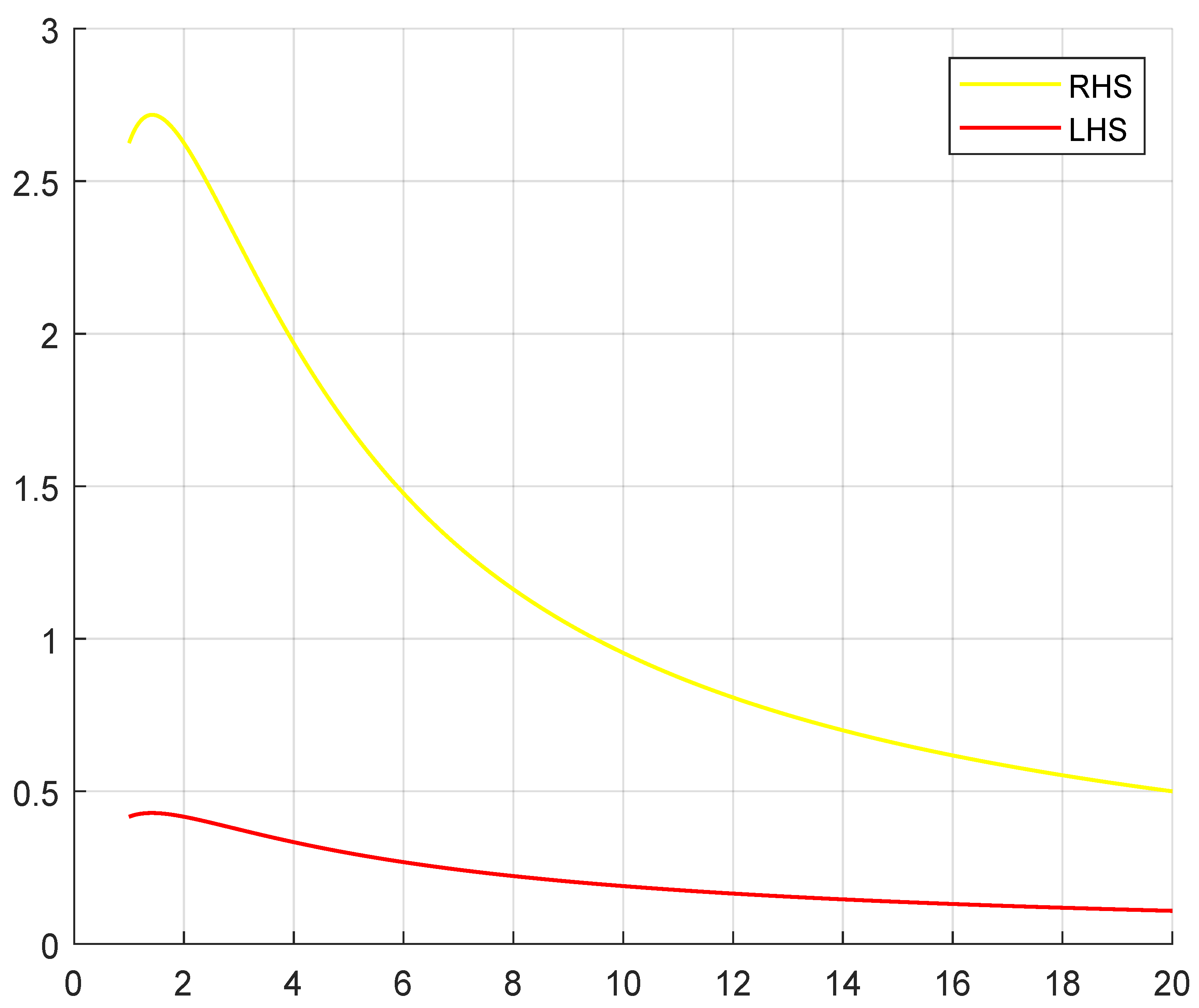
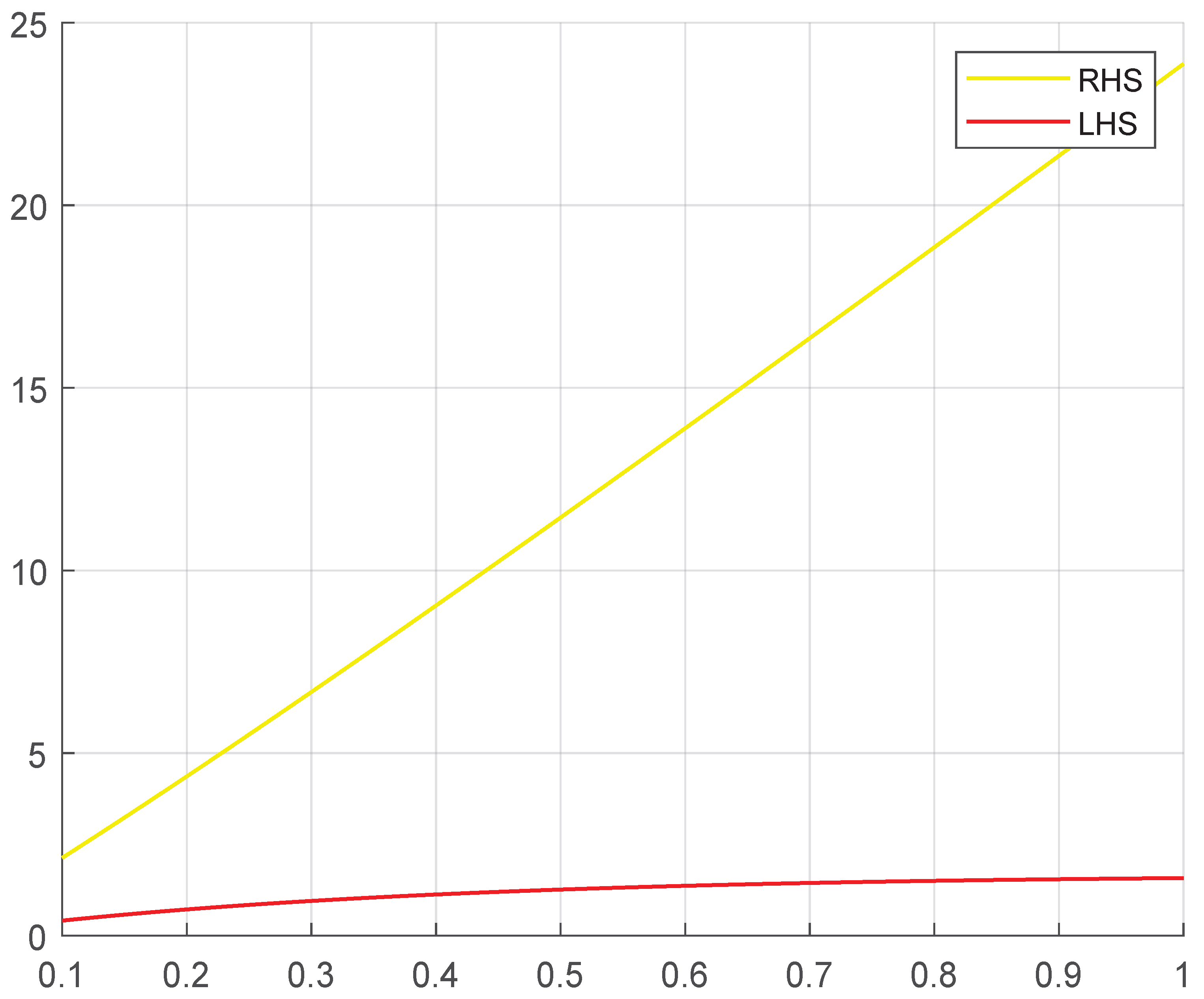
5. Examples and Illustrations

Example 1.

Under the conditions of Theorem 4, if we take $\xi =2,$ $\partial =\alpha ,$ $\varphi \left(0\right)=1,$ and $\beta =0,$ then we have

$$\begin{array}{cc} & \left|{\displaystyle \frac{f\left({\delta }_1+{\delta }_2-{\varkappa }_1\right)+f\left({\delta }_1+{\delta }_2-{\hslash }_1\right)}{2}}-{\displaystyle \frac{\alpha }{2{\left[{\hslash }_1-{\varkappa }_1\right]}^{\alpha }}}\right.\hfill \\ & \left.\times {\int }_{{\delta }_1+{\delta }_2-{\hslash }_1}^{{\delta }_1+{\delta }_2-{\varkappa }_1}\left\{{\left[\left({\delta }_1+{\delta }_2-{\varkappa }_1\right)-u\right]}^{\alpha -1}+{\left[u-\left({\delta }_1+{\delta }_2-{\hslash }_1\right)\right]}^{\alpha -1}\right\}f\left(u\right)du\right|\hfill \\ \le & {\displaystyle \frac{\left|{\hslash }_1-{\varkappa }_1\right|}{\alpha +1}}\left(1-{\displaystyle \frac{1}{2^{\alpha }}}\right)\left\{\left|f^{\prime }\left({\delta }_1\right)\right|+\left|f^{\prime }\left({\delta }_2\right)\right|-{\displaystyle \frac{\left(\left|f^{\prime }\left({\varkappa }_1\right)\right|+\left|f^{\prime }\left({\hslash }_1\right)\right|\right)}{2}}\right\}.\hfill \end{array}$$

In addition, ${\delta }_1=1,$ ${\delta }_2=4,$ ${\varkappa }_1=3,$ ${\hslash }_1=2,$ and $f\left(\varkappa \right)={\displaystyle \frac{{\varkappa }^3}{3}},$ $f^{\prime }\left(\varkappa \right)={\varkappa }^2.$ Then, it can be seen that

$$\left|{\displaystyle \frac{35}{6}}-{\displaystyle \frac{35{\alpha }^3+195{\alpha }^2+340\alpha +210}{6(\alpha +1)(\alpha +2)(\alpha +3)}}\right|\le {\displaystyle \frac{21}{2}}{\displaystyle \frac{1}{\alpha +1}}\left(1-{\displaystyle \frac{1}{2^{\alpha }}}\right).$$

The following graph (Figure 1) illustrates the comparison between the left and right sides of Theorem 4.

Example 2.

Under the conditions of Theorem 5, if we choose $\xi =2,$ $\partial =\alpha ,$ $\varphi \left(0\right)=1,$ and $\beta =0,$ then we have

$$\begin{array}{cc} & \left|{\displaystyle \frac{f\left({\delta }_1+{\delta }_2-{\varkappa }_1\right)+f\left({\delta }_1+{\delta }_2-{\hslash }_1\right)}{2}}-{\displaystyle \frac{\alpha }{2{\left[{\hslash }_1-{\varkappa }_1\right]}^{\alpha }}}\right.\hfill \\ & \left.\times {\int }_{{\delta }_1+{\delta }_2-{\hslash }_1}^{{\delta }_1+{\delta }_2-{\varkappa }_1}\left\{{\left[\left({\delta }_1+{\delta }_2-{\varkappa }_1\right)-u\right]}^{\alpha -1}+{\left[u-\left({\delta }_1+{\delta }_2-{\hslash }_1\right)\right]}^{\alpha -1}\right\}f\left(u\right)du\right|\hfill \\ \le & {\displaystyle \frac{\alpha {\left({\hslash }_1-{\varkappa }_1\right)}^2}{2}}\left\{\left[\left|f^{\prime \prime }\left({\delta }_1\right)\right|+\left|f^{\prime \prime }\left({\delta }_2\right)\right|\right]-{\displaystyle \frac{1}{2(\alpha +1)(\alpha +2)}}\left(\left|f^{\prime \prime }\left({\varkappa }_1\right)\right|+\left|f^{\prime \prime }\left({\hslash }_1\right)\right|\right)\right\}.\hfill \end{array}$$

In addition, ${\delta }_1=1,$ ${\delta }_2=4,$ ${\varkappa }_1=3,$ ${\hslash }_1=2,$ and $f\left(\varkappa \right)={\displaystyle \frac{{\varkappa }^4}{4}},$ $f^{\prime \prime }\left(\varkappa \right)=3{\varkappa }^2.$ Then, it can be seen that

$$\left|{\displaystyle \frac{97}{8}}-{\displaystyle \frac{97{\alpha }^4+894{\alpha }^3+2867{\alpha }^2+3942\alpha +2328}{8(\alpha +1)(\alpha +2)(\alpha +3)(\alpha +4)}}\right|\le {\displaystyle \frac{\alpha }{2}}\left\{51-{\displaystyle \frac{39}{2(\alpha +1)(\alpha +2)}}\right\}.$$

The following graph (Figure 2) illustrates the comparison between the left and right sides of Theorem 5.

6. Conclusions

The Raina function has been subjected to substantial examination and advancement by several mathematicians since its association with the fractional integral operator was identified. A variety of beneficial fractional integral operators can be obtained by selecting particular values for the coefficient $\varphi \left(k\right)$. Researchers in this field are currently carrying out extensive studies of the popular $\mathcal{H}-\mathcal{H}$ inequality. In numerical integration, this inequality serves as a tool for error estimates. It provides estimates for the integral mean of the convex function and ensures that the convex function is integrable. Furthermore, it has been established for many convex functions, with special attention on s-type convex, exponential convex, composite convex, coordinate convex, etc. Another significant inequality associated with convex functions is the Mercer inequality. This inequality has recently been the focus of much attention, resulting in numerous generalizations and conclusions. In this paper, the concept of majorization is employed to derive the combined $\mathcal{H}-\mathcal{H}$ and Mercer inequalities within the framework of fractional calculus. Firstly, we have obtained two generalized $\mathcal{H}-\mathcal{H}-\mathcal{M}$ inequalities using majorization. Additionally, novel and existing results in the literature were achieved by giving special values of $\xi$, $\partial ,$ $\varphi$, and $\beta$ to the results obtained. Secondly, we have developed two new identities (namely Lemmas 1 and 2). A significant finding of the present paper is that novel results concerning functions for which the second derivative is convex have been established. Researchers interested in this area can utilize different methods (such as Hölder, power-mean and Young inequalities, especially corollaries), different convex functions or concave functions, and new operators to obtain more general results (for examples, see Lemma 2.5 and Lemma 2.9 in [53]). In this regard, the presented consequences and methods in this paper may explore further investigation in this area by mathematicians.

References

1. Tseng, K.L.; Hwang, S.R.; Dragomir, S.S. Fejér-type inequalities (II). Math. Slovaca 2017, 67, 109–120. [Google Scholar] [CrossRef]
2. Alomari, M.; Darus, M.; Dragomir, S.S.; Cerone, P. Ostrowski type inequalities for functions whose derivatives are s-convex in the second sense. App. Math. Lett. 2010, 23, 1071–1076. [Google Scholar] [CrossRef]
3. Bai, R.F.; Qi, F.; Xi, B.Y. Hermite-Hadamard type inequalities for the m-and (α, m)-logarithmically convex functions. Filomat 2013, 27, 1–7. [Google Scholar] [CrossRef]
4. Butt, S.I.; Nadeem, M.; Tariq, M.; Aslam, A. New integral type inequalities via Raina-convex functions and its applications. Com. Fac. Sci. Uni. Ankara Ser. A1 Math. Stat. 2021, 70, 1011–1035. [Google Scholar] [CrossRef]
5. Butt, S.I.; Umar, M.; Khan, D.; Seol, Y.; Tipurić-Spužević, S. Hermite-Hadamard-Type Inequalities for Harmonically Convex Functions via Proportional Caputo-Hybrid Operators with Applications. Fractal Fract. 2025, 9, 77. [Google Scholar] [CrossRef]
6. Sarikaya, M.Z.; Set, E.; Yaldiz, H.; Başak, N. Hermite-Hadamard’s inequalities for fractional integrals and related fractional inequalities. Math. Comp. Model. 2013, 57, 2403–2407. [Google Scholar] [CrossRef]
7. Özdemir, M.E.; Kavurmaci, H.; Akdemir, A.O.; Avci, M. Inequalities for convex and s-convex functions on Δ = [a, b] × [c, d]. J. Ineq. App. 2012, 20, 1–19. [Google Scholar] [CrossRef]
8. Özdemir, M.E.; Yıldız, Ç.; Akdemir, A.O.; Set, E. On some inequalities for s-convex functions and applications. J. Ineq. App. 2013, 111, 333. [Google Scholar] [CrossRef]
9. Yıldız, Ç.; Rahman, G.; Cotîrlă, L.-I. On Further Inequalities for Convex Functions via Generalized Weighted-Type Fractional Operators. Fractal Fract. 2023, 7, 513. [Google Scholar] [CrossRef]
10. İşcan, İ. Hermite-Hadamard type inequalities for harmonically convex functions. Hacet. J. Math. Stat. 2014, 43, 935–942. [Google Scholar] [CrossRef]
11. Dragomir, S.S.; Agarwal, R. Two inequalities for differentiable mappings and applications to special means of real numbers and to trapezoidal formula. App. Math. Lett. 1998, 11, 91–95. [Google Scholar] [CrossRef]
12. Pearce, C.E.; Pečarić, J. Inequalities for differentiable mappings with application to special means and quadrature formulae. App. Math. Lett. 2000, 13, 51–55. [Google Scholar] [CrossRef]
13. Sarikaya, M.Z.; Saglam, A.; Yıldırım, H. New inequalities of Hermite-Hadamard type for functions whose second derivatives absolute values are convex and quasi-convex. Inter. J. Open Probl. Com. Sci. Math. 2012, 5, 3. [Google Scholar] [CrossRef]
14. Sarikaya, M.Z.; Kiris, M.E. Some new inequalities of Hermite-Hadamard type for s-convex functions. Miskolc Math. Notes 2015, 16, 491–501. [Google Scholar] [CrossRef]
15. Yildiz, Ç.; Özdemir, M.E. On generalized inequalities of Hermite-Hadamard type for convex functions. Inter. J. Anal. Appl. 2017, 14, 52–63. [Google Scholar]
16. Kadakal, M.; İşcan, İ.; Agarwal, P.; Jleli, M. Exponential trigonometric convex functions and Hermite-Hadamard type inequalities. Math. Slovaca 2021, 71, 43–56. [Google Scholar] [CrossRef]
17. Khan, M.A.; Chu, Y.; Khan, T.U.; Khan, J. Some new inequalities of Hermite-Hadamard type for s-convex functions with applications. Open Math. 2017, 15, 1414–1430. [Google Scholar] [CrossRef]
18. Khan, M.B.; Macías-Díaz, J.E.; Treanţă, S.; Soliman, M.S.; Zaini, H.G. Hermite-Hadamard Inequalities in Fractional Calculus for Left and Right Harmonically Convex Functions via Interval-Valued Settings. Fractal Fract. 2022, 6, 178. [Google Scholar] [CrossRef]
19. Mohammed, P.O.; Brevik, I. A New Version of the Hermite-Hadamard Inequality for Riemann-Liouville Fractional Integrals. Symmetry 2020, 12, 610. [Google Scholar] [CrossRef]
20. Peng, Y.; Özcan, S.; Du, T. Symmetrical Hermite-Hadamard type inequalities stemming from multiplicative fractional integrals. Chaos Solitons Fractals 2024, 183, 114960. [Google Scholar] [CrossRef]
21. Mohammed, P.O.; Abdeljawad, T.; Zeng, S.; Kashuri, A. Fractional Hermite-Hadamard Integral Inequalities for a New Class of Convex Functions. Symmetry 2020, 12, 1485. [Google Scholar] [CrossRef]
22. Moradi, H.R.; Omidvar, M.E.; Adil, K.M.; Nikodem, K. Around Jensen’s inequality for strongly convex functions. Aequationes Math. 2018, 92, 25–37. [Google Scholar] [CrossRef]
23. Khan, S.; Khan, M.A.; Chu, Y.M. New converses of Jensen inequality via Green functions with applications. Rev. Real Academia Cienc. Exactas Fis. Nat. Ser. A Mat. 2020, 114, 114. [Google Scholar] [CrossRef]
24. Mercer, A.M. A variant of Jensen’s inequality. J. Inequal. Pure Appl. Math. 2003, 4, 73. [Google Scholar]
25. Kian, M.; Moslehian, M.S. Refinements of the operator Jensen-Mercer inequality. Electron. J. Linear Algebra 2013, 26, 742–753. [Google Scholar] [CrossRef]
26. Khan, M.A.; Pecaric, J. New refinements of the Jensen-Mercer inequality associated to positive n-tuples. Armen. J. Math. 2020, 12, 1–12. [Google Scholar] [CrossRef]
27. Moradi, H.R.; Furuichi, S. Improvement and generalization of some Jensen-Mercer-type inequalities. J. Math. Inequal. 2020, 14, 377–383. [Google Scholar] [CrossRef]
28. Ali, M.A.; Sitthiwirattham, T.; Köbis, E.; Hanif, A. Hermite-Hadamard-Mercer Inequalities Associated with Twice-Differentiable Functions with Applications. Axioms 2024, 13, 114. [Google Scholar] [CrossRef]
29. Abbasi, M.; Morassaei, A.; Mirzapour, F. Jensen-Mercer Type Inequalities for Operator h-Convex Functions. Bull. The Iranian Math. Soc. 2022, 48, 2441–2462. [Google Scholar] [CrossRef]
30. Dragomir, S.S.; Agarwal, R.P.; Barnett, N.S. Inequalities for beta and gamma functions via some classical and new integral inequalities. RGMIA Res. Rep. Collect. 1999, 2, 3. [Google Scholar] [CrossRef]
31. Öğulmüş, H.; Sarıkaya, M.Z. Hermite-Hadamard-Mercer type inequalities for fractional integrals. Filomat 2021, 35, 2425–2436. [Google Scholar] [CrossRef]
32. Ali, M.A.; Hussain, T.; Iqbal, M.Z.; Ejaz, F. Inequalities of Hermite-Hadamard-Mercer type for convex functions via k-fracttional integrals. Inter. J. Math. Mod. Comp. 2020, 10, 227–238. [Google Scholar]
33. Vivas-Cortez, M.; Awan, M.U.; Javed, M.Z.; Kashuri, A.; Noor, M.A.; Noor, K.I.; Vlora, A. Some new generalized k-fractional Hermite-Hadamard-Mercer type integral inequalities and their applications. AIMS Math. 2022, 7, 3203–3220. [Google Scholar] [CrossRef]
34. Sahoo, S.K.; Hamed, Y.S.; Mohammed, P.O.; Kodamasingh, B.; Nonlaopon, K. New midpoint type Hermite-Hadamard-Mercer inequalities pertaining to Caputo-Fabrizio fractional operators. Alex. Eng. J. 2023, 65, 689–698. [Google Scholar] [CrossRef]
35. Çiftci, Z.; Coşkun, M.; Yildiz, Ç.; Cotîrlă, L.-I.; Breaz, D. On New Generalized Hermite-Hadamard-Mercer-Type Inequalities for Raina Functions. Fractal Fract. 2024, 8, 472. [Google Scholar] [CrossRef]
36. Liu, J.B.; Butt, S.I.; Nasir, J.; Aslam, A.; Fahad, A.; Soontharanon, J. Jensen-Mercer variant of Hermite-Hadamard type inequalities via Atangana-Baleanu fractional operator. AIMS Math. 2022, 7, 2123–2141. [Google Scholar] [CrossRef]
37. Butt, S.I.; Nasir, J.; Qaisar, S.; Abualnaja, K.M. k-Fractional variants of Hermite-Mercer-type inequalities via s-convexity with applications. J. Func. Spac. 2021, 1–5. [Google Scholar] [CrossRef]
38. Sitthiwirattham, T.; Vivas-Cortez, M.; Ali, M.A.; Budak, H.; Avcı, I. A study of fractional Hermite-Hadamard-Mercer inequalities for differentiable functions. Fractals 2024, 32, 2440016. [Google Scholar] [CrossRef]
39. Vivas-Cortez, M.; Javed, M.Z.; Awan, M.U.; Noor, M.A.; Dragomir, S.S. Bullen-Mercer type inequalities with applications in numerical analysis. Alex. Engin. J. 2024, 96, 15–33. [Google Scholar] [CrossRef]
40. Raina, R.K. On generalized Wright’s hypergeometric functions and fractional calculus operators. East Asian Math. J. 2005, 21, 191–203. [Google Scholar]
41. Agarwal, R.P.; Luo, M.J.; Raina, R.K. On Ostrowski Type Inequalities. Fasc. Math. 2016, 56, 5–27. [Google Scholar] [CrossRef]
42. Set, E.; Çelik, B.; Özdemir, M.E.; Aslan, M. Some New Results on Hermite-Hadamard-Mercer-Type Inequalities Using a General Family of Fractional Integral Operators. Fractal Fract. 2021, 5, 68. [Google Scholar] [CrossRef]
43. Budak, H.; Usta, F.; Sarikaya, M.Z.; Özdemir, M.E. On generalization of midpoint type inequalities with generalized fractional integral operators. Rev. Real Acad. Cienc. Exactas Fisicas Nat. Ser. Mat. 2019, 113, 769–790. [Google Scholar] [CrossRef]
44. Coşkun, M.; Yildiz, Ç.; Cotîrlă, L.-I. Novel Estimations of Hadamard-Type Integral Inequalities for Raina’s Fractional Operators. Fractal Fract. 2024, 8, 302. [Google Scholar] [CrossRef]
45. Srivastava, H.M. A Survey of Some Recent Developments on Higher Transcendental Functions of Analytic Number Theory and Applied Mathematics. Symmetry 2021, 13, 2294. [Google Scholar] [CrossRef]
46. Yaldiz, H.; Sarikaya, M.Z. On the Hermite-Hadamard type inequalities for fractional integral operator. Kragujevac J. Math. 2020, 44, 369–378. [Google Scholar] [CrossRef]
47. Wang, B.-Y. Foundations of Majorization Inequalities; Beijing Normal University Press: Beijing, China, 1990. [Google Scholar]
48. Marshall, A.W.; Olkin, I.; Arnold, B.C. Inequalities: Theory of Majorization and Its Applications, 2nd ed.; Springer Series in Statistics; Springer: London, UK, 2009. [Google Scholar]
49. Khan, M.A.; Latif, N.; Pečarić, P. Generalization of majorization theorem. Nonlinear Func. Anal. App. 2015, 20, 301–327. [Google Scholar] [CrossRef]
50. Wu, S.; Khan, M.A.; Haleemzai, H.U. Refinements of Majorization Inequality Involving Convex Functions via Taylor’s Theorem with Mean Value form of the Remainder. Mathematics 2019, 7, 663. [Google Scholar] [CrossRef]
51. Saeed, T.; Khan, M.A.; Ullah, H. Refinements of Jensen’s inequality and applications. Aims Math. 2022, 7, 5328–5346. [Google Scholar] [CrossRef]
52. Butt, S.I.; Javed, I.; Agarwal, P.; Nieto, J.J. Newton-Simpson-type inequalities via majorization. J. Ineq. Appl. 2023, 2023, 16. [Google Scholar] [CrossRef]
53. Faisal, S.; Khan, M.A.; Iqbal, S. Generalized Hermite-Hadamard-Mercer type inequalities via majorization. Filomat 2022, 36, 469–483. [Google Scholar] [CrossRef]
54. Ding, X.; Zuo, X.; Butt, S.I.; Farooq, R.; Tipurić-Spužević, S. New majorized fractional Simpson estimates. Axioms 2023, 12, 965. [Google Scholar] [CrossRef]
55. Faisal, S.; Adil Khan, M.; Khan, T.U.; Saeed, T.; Alshehri, A.M.; Nwaeze, E.R. New “Conticrete” Hermite-Hadamard-Jensen-Mercer Fractional Inequalities. Symmetry 2022, 14, 294. [Google Scholar] [CrossRef]
56. Faisal, S.; Khan, M.A.; Khan, T.U.; Saeed, T.; Mohammad Mahdi Sayed, Z.M. Unifications of continuous and discrete fractional inequalities of the Hermite-Hadamard-Jensen-Mercer type via majorization. J. Func. Spaces 2022, 1, 6964087. [Google Scholar] [CrossRef]
57. Khan, M.A.; Faisal, S. Derivation of conticrete Hermite-Hadamard-Jensen-Mercer inequalities through k-Caputo fractional derivatives and majorization. Filomat 2024, 38, 3389–3413. [Google Scholar] [CrossRef]
58. Saeed, T.; Khan, M.A.; Faisal, S.; Alsulami, H.H.; Alhodaly, M.S. New conticrete inequalities of the Hermite-Hadamard-Jensen-Mercer type in terms of generalized conformable fractional operators via majorization. Demonstr. Math. 2023, 56, 20220225. [Google Scholar] [CrossRef]
59. Wu, S.; Khan, M.A.; Faisal, S.; Saeed, T.; Nwaeze, E.R. Derivation of Hermite-Hadamard-Jensen-Mercer conticrete inequalities for Atangana-Baleanu fractional integrals by means of majorization. Demonstr. Math. 2024, 57, 20240024. [Google Scholar] [CrossRef]
60. Niezgoda, M. A generalization of Mercer’s result on convex functions. Nonlinear Anal. 2009, 71, 2771–2779. [Google Scholar] [CrossRef]
61. Set, E.; Dragomir, S.S.; Gözpınar, A. Some generalized Hermite-Hadamard type inequalities involving fractional integral operator for functions whose second derivatives in absolute value are s-convex. Acta Math. Univ. Comen. 2019, 88, 87–100. [Google Scholar]
Figure 1. The graph of Theorem 4 for the choice of order α [ 1 , 20 ] is presented in Figure 1.
Fractalfract 09 00343 g001
Figure 2. The graph of Theorem 5 for the choice of order α [ 0 , 1 ] is presented in Figure 1.
Fractalfract 09 00343 g002
Disclaimer/Publisher’s Note: The statements, opinions and data contained in all publications are solely those of the individual author(s) and contributor(s) and not of MDPI and/or the editor(s). MDPI and/or the editor(s) disclaim responsibility for any injury to people or property resulting from any ideas, methods, instructions or products referred to in the content.