Article

A Non-Standard Finite Difference Scheme for Time-Fractional Singularly Perturbed Convection–Diffusion Problems

by
Pramod Chakravarthy Podila
1,†,
Rahul Mishra
1,† and
Higinio Ramos
2,*
1
Visvesvaraya National Institute of Technology, Nagpur 440010, India
2
Scientific Computing Group, Universidad de Salamanca, Plaza de la Merced, 37008 Salamanca, Spain
*
Author to whom correspondence should be addressed.
These authors contributed equally to this work.
Fractal Fract. 2025, 9(6), 333; https://doi.org/10.3390/fractalfract9060333
Submission received: 3 March 2025 / Revised: 6 May 2025 / Accepted: 21 May 2025 / Published: 23 May 2025

Abstract

This paper introduces a stable non-standard finite difference (NSFD) method to solve time-fractional singularly perturbed convection–diffusion problems. The fractional derivative in time is defined in the Caputo sense. The proposed method shows high efficiency when applied using a uniform mesh and can be easily extended to a Shishkin mesh in the spatial domain. We discuss error estimates to demonstrate the convergence of the numerical scheme. Additionally, various numerical examples are presented to illustrate the behavior of the solution for different values of the perturbation parameter ϵ and the order of the fractional derivative.

1. Introduction

Singularly perturbed differential equations have gained significant attention from researchers due to their extensive applications in science and engineering disciplines, including material science, biosciences, economics, neural networks, control theory, robotics, the oil industry, and finance. Partial differential equations (PDEs) are frequently used to model many physical phenomena. For a comprehensive discussion on singular perturbation problems (SPPs), refer to the work of Bender and Orszag [1], Nayfeh [2], and O’Malley [3]. While the literature on SPPs is extensive, we highlight some notable contributions related to singularly perturbed parabolic partial differential equations (SPPPDEs). For instance, Clavero et al. [4] proposed a parameter-uniform convergent method using a non-uniform mesh for SPPPDEs, and Kadalbajoo et al. [5] developed a B-spline collocation approach for singularly perturbed time-dependent convection–diffusion problems. Other important contributions include the hybrid numerical method for SPPPDEs proposed by Clavero et al. [6], the Bessel collocation method proposed by Yüzbasıa and Şahin [7], and the finite difference method for singularly perturbed parabolic reaction–diffusion problems proposed by Clavero and Gracia [8], while Bansal and Sharma [9] introduced an NSFD method for handling SPPPDEs with general shift arguments.
In recent years, fractional calculus has attracted a lot of attention due to its numerous applications in different fields. In particular, time-fractional singularly perturbed convection–diffusion equations have been widely used in modeling complex phenomena. Some notable applications include the following [10,11]:
  • Time-fractional singularly perturbed convection–diffusion models play a crucial role in modeling anomalous transport phenomena in biological systems. They are particularly effective in capturing subdiffusive behavior observed in complex environments such as cellular interiors. These models account for memory effects and accurately represent sharp concentration gradients, making them highly suitable for simulating processes like drug diffusion through tissues and intracellular signaling pathways.
  • Time-fractional singularly perturbed convection–diffusion equations are applied to model heat and mass transfer in advanced materials exhibiting memory-dependent behavior. They provide a more accurate representation of transport processes in materials like polymers and viscoelastic composites.
  • In porous media, time-fractional models effectively capture anomalous diffusion arising from the heterogeneous structure of material. They are especially valuable for simulating groundwater flow and contaminant transport, where conventional models often fail to reflect the intricate and non-uniform nature of the underlying flow dynamics.
This increasing focus is evident from the numerous studies conducted in this area. The concept of fractional derivatives was first introduced by Leibniz in 1695, and further developments were made by Riemann and Liouville, who laid the groundwork for fractional calculus. Foundational results in the theory of fractional differential equations have been extensively developed in the works of Podlubny [12], Kilbas et al. [13], Li and Zeng [14], and Cai and Li [15].
Several researchers have contributed to numerical methods for fractional PDEs. In order to solve time-fractional diffusion equations, Lin and Xu [16] created a finite difference scheme in conjunction with the Legendre spectral approach in space. Stynes et al. [17] introduced a graded mesh-based finite difference approach. A numerical approach was developed by Choudhary et al. [18] for time-fractional PDEs with time lag. Several numerical techniques have been proposed to obtain approximate solutions for time-fractional problems; see, for instance [19,20,21,22,23]. However, analytical solutions for time-fractional singularly perturbed PDEs are generally difficult to obtain. To address this, researchers have developed various numerical techniques. For instance, a finite difference approach was proposed by Kumar et al. [24] for time-fractional SPPPDEs with time lag. A Crank–Nicolson approach was developed by Kumie et al. [25] to solve time-fractional singularly perturbed delay PDEs. Sahoo and Gupta [26] introduced a uniform convergent numerical approach for solving time-fractional SPPPDEs. A second-order finite difference method was developed by Sahoo et al. [27] for solving time-fractional SPPPDEs. Worku and Duressa [28] proposed a numerical approach for solving SPPPDEs. An exponentially fitted operator-based scheme was developed by Tiruneh et al. [29] for solving time-fractional SPPPDEs. Recently, a novel fitted finite difference approach was proposed by Aniley and Duressa [30].
Inspired by these works, this paper aims to solve time-fractional SPPPDEs in the following form:
L y ( s , t ) D t α y ϵ y s s + a ( s , t ) y s + b ( s , t ) y = g ( s , t ) ,
where ( s , t ) D and D = Ω s × Ω t = ( 0 , 1 ) × ( 0 , T ] , with boundary conditions given as
y ( s , 0 ) = ϕ b ( s ) , for s Ω ¯ s , y ( 0 , t ) = ϕ l ( t ) , y ( 1 , t ) = ϕ r ( t ) for t Ω t ,
where D t α denotes the Caputo fractional derivative of the order α ( 0 , 1 ) [31] and 0 ϵ 1 is a small perturbation parameter. It is assumed that a ( s , t ) γ > 0 and b ( s , t ) 0 , while g ( s , t ) and the initial and boundary conditions are smooth and bounded in their respective domains. The solution of this model problem exhibits a boundary layer near s = 1 .
It is well known that classical numerical methods may fail to produce satisfactory results when ϵ 0 , unless a very fine mesh is considered, which significantly increases computational cost. Hence, it is crucial to develop an efficient numerical scheme for solving Problems (1)–(2) that maintains accuracy regardless of the value of the parameter ϵ . The primary aim of this study is to develop a parameter-uniform convergent numerical scheme for Problems (1)–(2). Two key challenges make the development of an approximate solution particularly difficult:
  • The time-fractional derivative introduces weak singularities in the solution at the initial time [17].
  • The perturbation parameter ϵ causes the formation of boundary layers in the solution [1].
To address these, we use a L 1 scheme for the temporal derivative, followed by the application of an NSFD approach to solve the semi-discretized problem. This method performs exceptionally well for small values of ϵ on a uniform mesh. The key benefits of the proposed scheme include the following:
(i)
It produces oscillation-free solutions on a uniform mesh.
(ii)
It delivers more accurate results than traditional methods.
(iii)
It maintains convergence order even for very small values of ϵ .
(iv)
It is unconditionally stable and exhibits parameter-uniform convergence.
The rest of this paper is organized as follows: Section 2 introduces key definitions and a priori estimates. The numerical scheme is detailed in Section 3. Convergence estimates are provided in Section 4, followed by a discussion of numerical results in Section 5. The paper concludes with Section 6.

2. Some Preliminaries

Here, we present some fundamental definitions of fractional derivatives which will be employed in the development of the scheme for Problems (1)–(2).
Definition 1 
([12]). Consider z a complex number with ( z ) > 0 . The Gamma function for such z is defined as
Γ ( z ) = 0 s z 1 e s d s .
Definition 2 
([31]). Given n N , the Caputo fractional derivative of a function, f ( s ) , of the order α ( n 1 , n ) is defined as
D 0 α f ( s ) = 1 Γ ( n α ) 0 s ( s p ) n α 1 f ( n ) ( p ) d p .
Definition 3 
([31]). For every n N , the Caputo fractional partial derivative of the order α of a function, y ( s , t ) , is given by
α y ( s , t ) t α = 1 Γ ( n α ) 0 t n y ( s , p ) p n ( t p ) n α 1 d p if α ( n 1 , n ) , n y ( s , t ) t n if α = n .
Theorem 1 
([32]). Let Φ ( s , t ) and Ψ ( s , t ) be twice-differentiable functions in s and once-differentiable functions in t on D, satisfying
| L Φ ( s , t ) | L Ψ ( s , t ) , ( s , t ) D ,
| Φ ( s , t ) | Ψ ( s , t ) , ( s , t ) D ¯ D ,
where L is the operator defined in (1). Then,
| Φ ( s , t ) | Ψ ( s , t ) , ( s , t ) D ¯ .
Proof. 
According to the extreme value theorem, there exists ( s 1 , t 1 ) D ¯ such that
( Φ Ψ ) ( s 1 , t 1 ) = max ( s , t ) D ¯ ( Φ Ψ ) ( x , t ) .
We proceed by contradiction. Assume that ( Φ Ψ ) ( s 1 , t 1 ) > 0 . Applying the operator L to the function ( Φ Ψ ) , we obtain
L ( Φ Ψ ) ( s , t ) = D t α ( Φ Ψ ) ( s , t ) ϵ ( Φ Ψ ) s s ( s , t ) + a ( s , t ) ( Φ Ψ ) s ( s , t ) + b ( s , t ) ( Φ Ψ ) ( s , t ) .
Since ( s 1 , t 1 ) is a point of maximum, we have
D t α ( Φ Ψ ) | ( s 1 , t 1 ) 0 , ( Φ Ψ ) s | ( s 1 , t 1 ) = 0 , ( Φ Ψ ) s s | ( s 1 , t 1 ) < 0 .
This implies that
L ( Φ Ψ ) ( s 1 , t 1 ) > 0 ,
which is a contradiction. Therefore,
Φ ( s , t ) Ψ ( s , t ) , ( s , t ) D ¯ .
Similarly, let ( s 2 , t 2 ) D ¯ be such that
( Φ Ψ ) ( s 2 , t 2 ) = max ( s , t ) D ¯ ( Φ Ψ ) ( s , t ) ,
and assume that ( Φ Ψ ) ( s 2 , t 2 ) > 0 . By similar reasoning, we obtain
Φ ( s , t ) Ψ ( s , t ) , ( s , t ) D ¯ .
Combining (6) and (7), we obtain
| Φ ( s , t ) | Ψ ( s , t ) , ( s , t ) D ¯ ,
which completes the proof. □
Lemma 1 
([32]). There exists a constant, K, independent of ϵ such that for sufficiently small positive values of ϵ, the following relations hold throughout D ¯ :
| y ( s , t ) ϕ b ( s ) | K t , | y ( s , t ) ϕ l ( t ) | K s .
Proof. 
Let Φ ( s , t ) = y ( s , t ) ϕ b ( s ) . Then,
L Φ ( s , t ) = g ( s , t ) D t α ϕ b ( s ) + ϵ ( ϕ b ( s ) ) s s a ( s , t ) ( ϕ b ( s ) ) s b ( s , t ) ϕ b ( s ) ,
with
Φ ( s , 0 ) = 0 , for 0 < s < 1 ,
Φ ( 0 , t ) = ϕ l ( t ) ϕ b ( 0 ) , Φ ( 1 , t ) = ϕ r ( t ) ϕ b ( 1 ) , for 0 t 1 .
The hypotheses imply that for 0 t 1 ,
| Φ ( 0 , t ) | = | ϕ l ( t ) ϕ b ( 0 ) | C t , | Φ ( 1 , t ) | = | ϕ r ( t ) ϕ b ( 1 ) | C t ,
for some constants, C and C .
Let Ψ ( s , t ) = K t for any constant, K. Then,
L Ψ ( s , t ) = K Γ ( 2 α ) t 1 α + K t b ( s , t ) ,
with
Ψ ( s , 0 ) = 0 , for 0 < s < 1 ,
Ψ ( 0 , t ) = K t , Ψ ( 1 , t ) = K t , for 0 t 1 .
Using the given data and choosing a sufficiently large K, and applying Theorem 1 to Φ ( s , t ) and Ψ ( s , t ) , we obtain the desired result. The proof for the second inequality is analogous. □
Lemma 2 
([24]). The solution of Problems (1)–(2) is bounded by
| y ( s , t ) | K , ( s , t ) D ¯ .
Proof. 
According to Lemma (1), we have
| y ( s , t ) | | ϕ b ( s ) | | y ( s , t ) ϕ b ( s ) | K t , | y ( s , t ) | K t + | ϕ b ( s ) | , ( s , t ) D ¯ .
Since t ( 0 , T ] and ϕ b C 2 ( D ¯ ) , the function K t + | ϕ b ( s ) | is bounded. Therefore, | y ( s , t ) | K , for all ( s , t ) D ¯ . □
Lemma 3 
(Maximum Principle [25]). Let ψ ( s , t ) C 2 ( D ) C 0 ( D ¯ ) with L ψ ( s , t ) 0 in D and ψ ( s , t ) 0 for all ( s , t ) Γ = { 0 } × Ω t { 1 } × Ω t Ω ¯ s × { 0 } . Then ψ ( s , t ) 0 for all ( s , t ) D ¯ .
Proof. 
Let ( s 1 , t 1 ) D ¯ be such that
ψ ( s 1 , t 1 ) = min ( s , t ) D ¯ ψ ( s , t ) .
We proceed by contradiction. Assume that ψ ( s 1 , t 1 ) < 0 . Then, ( s 1 , t 1 ) Γ , meaning that ( s 1 , t 1 ) D . Applying the operator L to ψ ( s , t ) , we obtain
L ψ ( s , t ) = D t α ψ ( s , t ) ϵ ψ s s ( s , t ) + a ( s , t ) ψ s ( s , t ) + b ( s , t ) ψ ( s , t ) .
Since ( s 1 , t 1 ) is a point of minima, we have D t α ψ ( s 1 , t 1 ) 0 , ψ s ( s 1 , t 1 ) = 0 , ψ s s ( s 1 , t 1 ) 0 , and b ( s 1 , t 1 ) 0 for ( s 1 , t 1 ) D ¯ . Therefore,
L ψ ( s 1 , t 1 ) < 0 ,
which contradicts the assumption that L ψ ( s , t ) 0 in D. Hence, ψ ( s , t ) 0 for all ( s , t ) D ¯ . □
Remark 1. 
The operator satisfies the maximum principle and, consequently, L 1 K .
Lemma 4 
(Uniqueness [26]). For α ( 0 , 1 ) and each ϵ > 0 , Problems (1)–(2) have a unique solution.
Proof. 
Consider two functions, ψ 1 ( s , t ) and ψ 2 ( s , t ) , satisfying (1)–(2) such that
ψ ( s , t ) = ψ 1 ( s , t ) ψ 2 ( s , t ) .
Applying the operator L to ψ ( s , t ) , we obtain
L ψ ( s , t ) = D t α ψ ( s , t ) ϵ ψ s s ( s , t ) + a ( s , t ) ψ s ( s , t ) + b ( s , t ) ψ ( s , t ) , ( s , t ) D .
According to the maximum principle (Lemma (3)), we have ψ 0 and ψ 0 , which implies that ψ = ψ 1 ψ 2 = 0 . Thus, Problems (1)–(2) have a unique solution. □
Theorem 2 
([26]). Consider the vector space V ( ρ ) = v L 2 ( 0 , 1 ) : i = 1 λ i 2 ρ | ( v , Φ i ) | 2 < , ρ 0 , where, ( . , . ) denotes the inner product in the Hilbert space L 2 ( 0 , 1 ) . λ i are the eigenvalues, and Φ i denote the eiassociated normalized eigen functions of the following two-point boundary value problem
Φ i : = ϵ Φ i + b 1 Φ i = λ i Φ i on ( 0 , 1 ) with Φ i ( 0 ) = Φ i ( 1 ) = 0 .
For each t ( 0 , T ] , consider the functions Φ , g V ( 5 / 2 ) and g t ( . , t ) , g t t ( . , t ) V ( 1 / 2 ) which satisfy the following condition:
g ( . , t ) 5 / 2 + g t ( . , t ) 1 / 2 + t η g t t ( . , t ) 1 / 2 K , t ( 0 , T ] ,
where η < 1 and K is a constant. Then, the solution y to Problems (1)–(2) satisfies the following bounds for its temporal and spatial derivatives:
j y ( s , t ) t j K ( 1 + t α j ) , for j = 0 , 1 , 2 , i y ( s , t ) s i K ( 1 + ϵ i ) , for i = 0 , 1 , 2 , 3 ,
for all ( s , t ) Ω ¯ s × Ω ¯ t , where K is a generic positive constant.
Proof. 
To prove this theorem, we begin by applying the transformation y ( s , t ) = u ( s , t ) + ξ ( s , t ) , where ξ ( s , t ) = ϕ r ( t ) ϕ l ( t ) s + ϕ l ( t ) in order to reformulate Problems (1)–(2) with homogeneous boundary conditions. Next, we introduce another transformation, v ( s , t ) = u ( s , t ) exp 1 2 0 s a ( s , t ) ϵ d s , which transforms the problem into a normalized form. We then follow the approach outlined in [17] to obtain the temporal derivative bounds for the normalized problem. Finally, by reversing the transformations, the required bounds for the temporal derivatives of the original Problems (1)–(2) can be obtained. To derive bounds for the spatial derivatives, we introduce the stretched variable s ˜ = 1 s ϵ and apply the approach described in [33]. □

3. Numerical Scheme

Now, we will develop a numerical scheme for Problems (1)–(2). For this, the time derivative is approximated using the L 1 scheme, and an NSFD method is employed on a uniform spatial grid to solve the resulting system of ODEs.

3.1. Temporal Discretization

The time interval [ 0 , T ] is discretized uniformly into M subintervals with the step size Δ t = T M . The set Ω t M denotes all the mesh points in the time direction, i.e.,
Ω t M = { 0 = t 0 < t 1 < t 2 < < t M 1 < t M = 1 } .
From Definition (2), we have
v ( s , t j ) = α y ˜ ( s , t j ) t α = 1 Γ ( 1 α ) 0 t j y ˜ ( s , t j ) s ( t j p ) α d p .
Now, by using (8) in (1), we obtain
v ( s , t j ) ϵ 2 y ˜ ( s , t j ) s 2 + a ( s , t j ) y ˜ ( s , t j ) s + b ( s , t j ) y ˜ ( s , t j ) = g ( s , t j ) .
The semi-discretized problem mentioned above can be expressed as
ϵ 2 y ˜ ( s , t j ) s 2 + a ( s , t j ) y ˜ ( s , t j ) s + b ( s , t j ) y ˜ ( s , t j ) = g ( s , t j ) v ( s , t j ) ,
with
y ˜ ( s , 0 ) = ϕ b ( s ) , for s Ω ¯ s , y ˜ ( 0 , t j ) = ϕ l ( t j ) , y ˜ ( 1 , t j ) = ϕ r ( t j ) for t j Ω t M .
Now, we approximate v ( s , t j ) with the help of the following Lemma.
Lemma 5 
([24]). Let 0 < α < 1 and the function h ( t ) C 2 ( 0 , t j ] ; then, the following estimate holds:
| 1 Γ ( 1 α ) 0 t j h ( t ) ( t j t ) α d t | Δ t α Γ ( 2 α ) [ B j 1 h ( t 0 ) m = 1 j 1 B j m 1 B j m h ( t m ) + B 0 h ( t j ) ] + 1 Γ ( 2 α ) [ 1 α 12 ( 1 + 2 α ) + 2 2 α 2 α ] max 0 s t j | h ( t ) | Δ t 2 α ,
where B m = ( m + 1 ) 1 α m 1 α .
From Lemma (5), we have
v ( s , t j ) = Δ t α Γ ( 2 α ) B j 1 y ˜ ( s , t 0 ) m = 1 j 1 B j m 1 B j m y ˜ ( s , t m ) + B 0 y ˜ ( s , t j ) + T 1 ,
where T 1 K Δ t 2 α .
Now, by using (11) in (9), we obtain
ϵ 2 y ˜ ( s , t j ) s 2 + a ( s , t j ) y ˜ ( s , t j ) s + b ( s , t j ) y ˜ ( s , t j ) = g ( s , t j ) + Δ t α Γ ( 2 α ) × B j 1 y ˜ ( s , t 0 ) + m = 1 j 1 B j m 1 B j m y ˜ ( s , t m ) B 0 y ˜ ( s , t j ) .
We can express the above equation in operator form as
L ˜ y ˜ ( s , t j ) ϵ 2 y ˜ ( s , t j ) s 2 + a ( s , t j ) y ˜ ( s , t j ) s + w ( s , t j ) y ˜ ( s , t j ) = F ( s , t j ) .
with
y ˜ ( s , 0 ) = ϕ b ( s ) , for s Ω ¯ s , y ˜ ( 0 , t j ) = ϕ l ( t j ) , y ˜ ( 1 , t j ) = ϕ r ( t j ) for t j Ω t M ,
where
w ( s , t j ) = b ( s , t j ) + Δ t α B 0 Γ ( 2 α ) , F ( s , t j ) = g ( s , t j ) + Δ t α Γ ( 2 α ) B j 1 y ˜ ( s , t 0 ) + m = 1 j 1 B j m 1 B j m y ˜ ( s , t m ) .
Theorem 3 
([29]). The error estimates associated with the semi-discrete Problem (12), i.e., E j = y ( s , t j ) y ˜ ( s , t j ) , is given by
E j K Δ t 2 α .
Proof. 
The function y ( s , t j ) satisfies
L ˜ y ( s , t j ) = F ( s , t j ) .
Also, the solution y ˜ ( s , t j ) is sufficiently smooth; then, we have
L ˜ y ˜ ( s , t j ) = F ( s , t j ) + T 1 ,
L ˜ y ˜ ( s , t j ) = F ( s , t j ) + K Δ t 2 α .
Then, from (14) and (15), we have
L ˜ E j K Δ t 2 α E j K Δ t 2 α .
Lemma 6 
([28]). For every integer i [ 0 , 4 ] , the semi-discrete solution y ˜ ( s , t j ) corresponding to Equation (12) satisfies the following bounds:
| i y ˜ ( s , t j ) s i | K 1 + ϵ i exp γ ( 1 s ) ϵ , ( s , t j ) D ¯ .
Proof. 
See Lemma (4.4) of Bansal and Sharma [9] for the proof. □
The solution y ˜ of the semi-discrete Problem (12) and its derivatives must have strong bounds in order to guarantee ϵ -uniform convergence. We decompose the solution y ˜ into two components: a smooth component, y ˜ s m , and a singular component, y ˜ s i . These components satisfy the following bounds:
Lemma 7 
([26]). Let y ˜ ( s , t j ) be the solution of the semi-discrete Problem (12), such that
y ˜ ( s , t j ) = y ˜ s m ( s , t j ) + y ˜ s i ( s , t j ) , ( s , t j ) D ¯ .
Then, for every integer i [ 0 , 3 ] , the smooth component y ˜ s m satisfies
| i y ˜ s m s i | K 1 + ϵ 2 i exp γ ( 1 s ) ϵ , for all s Ω ¯ s ,
and the singular component y ˜ s i satisfies
| i y ˜ s i s i | K ϵ i exp γ ( 1 s ) ϵ , for all s Ω ¯ s .
Proof. 
The smooth component y ˜ s m corresponds to the solution of the associated non-homogeneous problem
L ˜ y ˜ s m ( s , t j ) = F ( s , t j ) , s Ω ¯ s ,
with
y ˜ s m ( s , 0 ) = y ˜ ( s , 0 ) , for s Ω ¯ s ,
y ˜ s m ( 0 , t j ) = y ˜ ( 0 , t j ) , y ˜ s m ( 1 , t j ) = y ˜ ( 1 , t j ) t j Ω ¯ t M .
and the singular component y ˜ s i corresponds to the solution of the associated homogeneous problem
L ˜ y ˜ s i ( s , t j ) = 0 , s Ω ¯ s ,
with
y ˜ s i ( s , 0 ) = 0 , for s Ω ¯ s ,
y ˜ s i ( 0 , t j ) = 0 , y ˜ s i ( 1 , t j ) = y ˜ ( 1 , t j ) y s m ( 1 , t j ) t j Ω ¯ t M .
Next, we examine a three-term asymptotic expansion for y ˜ s m expressed as
y ˜ s m = y 0 + ϵ y 1 + ϵ 2 y 2 , ( s , t j ) Ω ¯ s × Ω ¯ t M ,
where y 0 is the solution of the following reduced problem:
a ( s , t j ) y 0 ( s , t j ) s + w ( s , t j ) y 0 ( s , t j ) = F ( s , t j ) , ( s , t j ) Ω ¯ s × Ω ¯ t M ,
with
y 0 ( 0 , t j ) = y ˜ ( 0 , t j ) , for all t j Ω ¯ t M .
Additionally, y 1 , y 2 are the solutions of the differential equations and are given by
a ( s , t j ) y 1 ( s , t j ) s + w ( s , t j ) y 1 ( s , t j ) = 2 y 0 ( s , t j ) s 2 , ( s , t j ) Ω ¯ s × Ω ¯ t M ,
with
y 1 ( 0 , t j ) = 0 , t j Ω ¯ t M .
L ˜ y 2 ( s , t j ) = 2 y 1 ( s , t j ) s 2 , ( s , t j ) Ω ¯ s × Ω ¯ t M ,
with
y 2 ( 0 , t j ) = y 2 ( 1 , t j ) = 0 , t j Ω ¯ t M .
It is clear from (24) and (26) that y 0 and y 1 are solutions of the first-order linear differential equations with bounded coefficients which are independent from ϵ . Therefore, for every integer i [ 0 , 3 ] , we obtain the following bounds:
i y l s i K , for l = 0 , 1 .
Since y 2 is the solution of Problems (28) and (29), using Lemma (6), we obtain
| i y 2 s i | K 1 + ϵ i exp γ ( 1 s ) ϵ , s Ω ¯ s , i = 0 , 1 , 2 , 3 .
Now, using the estimates (30) and (31) in (23), we can obtain the desired estimates for y ˜ s m and its derivatives. We construct two barrier functions to determine the bounds for the singular part y ˜ s i as follows:
φ ± ( s , t j ) = | y ˜ s i ( 1 , t j ) | exp γ ( 1 s ) ϵ ± y ˜ s i ( s , t j ) , ( s , t j ) Ω ¯ s × Ω ¯ t M .
So, we have
φ ± ( 0 , t j ) = | y ˜ s i ( 1 , t j ) | exp γ ϵ 0 ,
φ ± ( 1 , t j ) = | y ˜ s i ( 1 , t j ) | ± y ˜ ( 1 , t j ) ( y 0 ( 1 , t j ) + ϵ y 1 ( 1 , t j ) ) 0 .
and
L ˜ φ ± ( s , t j ) = | y ˜ s i ( 1 , t j ) | γ ϵ ( γ + a ( s , t j ) ) + w ( s , t j ) 0 , s Ω ¯ s .
Using (33) in (32), we can conclude that
| y ˜ s i ( s , t j ) | K exp γ ( 1 s ) ϵ , s Ω ¯ s .
The following estimate is used to determine the constraints for the derivative of y ˜ s i ( s , t j ) :
y ˜ s i ( s , t j ) = 0 s H ( p , t j ) d p + μ 0 s exp ( B ( p , t j ) / ϵ ) d p , s Ω ¯ s ,
where μ can be determined with the help of boundary conditions for y ˜ s i ( 1 , t j ) and
H ( p , t j ) = 1 ϵ s 1 w ( p , t j ) y ˜ s i ( p , t j ) exp ( ( B ( s , t j ) B ( p , t j ) ) / ϵ ) d p , s Ω ¯ s ,
and
B ( s , t j ) = s 1 a ( p , t j ) d p , s Ω ¯ s .
By using the estimates obtained in (34) and the bound for a ( s , t ) , we can obtain the following bounds for H ( p , t j ) :
| H ( p , t j ) | K ϵ s 1 exp γ ( 1 p ) ϵ exp γ ( p s ) ϵ d p K ϵ exp γ ( 1 s ) ϵ , for all s Ω ¯ s .
From the above, we can conclude that
0 1 H ( p , t j ) d p K γ .
Now, let η = 0 1 exp ( B ( p , t j ) / ϵ ) d p K ϵ γ . By using the boundary condition y ˜ s i ( 1 , t j ) , we obtain the following estimate for μ :
| μ | = 1 η y ˜ s i ( 1 , t j ) 0 1 H ( p , t j ) d p K ϵ .
Now, by differentiating (35) with respect to s, we then have
y ˜ s i ( s , t j ) s = H ( s , t j ) + μ exp ( B ( s , t j ) / ϵ ) , s Ω ¯ s .
By using the estimate in (36) and the bound for μ , we obtain
y ˜ s i ( s , t j ) s K ϵ exp γ ( 1 s ) ϵ , s Ω ¯ s .
Similarly, the remaining bounds for the singular component y ˜ s i ( s , t j ) can be determined by using the estimates of y ˜ s i ( s , t j ) and y ˜ s i ( s , t j ) s . □

3.2. Space Discretization

3.2.1. Derivation of NSFD Scheme

Mickens [34] put forward a set of guidelines for creating NSFD schemes. By using these guidelines, one can obtain a unique finite difference model for PDEs. We use the uniform step size h = 1 / N to divide the space domain [ 0 , 1 ] into N equal subintervals. The set Ω s N represents all the mesh points in the space direction, which is defined as
Ω s N = { 0 = s 0 < s 1 < s 2 < < s N 1 < s N = 1 } .
Let y ˜ ( s , t j ) = y ˜ j ( s ) , a ( s , t j ) = a j ( s ) , w ( s , t j ) = w j ( s ) and F ( s , t j ) = F j ( s ) . Then, (12) can be written as
L ˜ y ˜ j ( s ) ϵ 2 y ˜ j ( s ) s 2 + a j ( s ) y ˜ j ( s ) s + w j ( s ) y ˜ j ( s ) = F j ( s ) .
Let y ^ be the approximate solution of (38) at the point s i . We consider the following homogeneous constant coefficient problem associated with Equation (38):
ϵ y ^ s s j ( s ) + a y ^ s j ( s ) + w y ^ j ( s ) = 0 ,
and
ϵ y ^ s s j ( s ) + a y ^ s j ( s ) = 0 .
Now, our aim is to derive a difference scheme that matches the general solution of Equation (39) at the grid points s i , and it is given by
y ^ i = A 1 exp ( λ 1 s i ) + B 1 exp ( λ 2 s i ) ,
where λ 1 and λ 2 are given by
λ 1 , 2 = a ± a 2 + 4 ϵ w 2 ϵ .
For second-order linear difference equations, we apply the theory of difference equations [9,34] to obtain
det y ^ i 1 j exp ( λ 1 s i 1 ) exp ( λ 2 s i 1 ) y ^ i j exp ( λ 1 s i ) exp ( λ 2 s i ) y ^ i + 1 j exp ( λ 1 s i + 1 ) exp ( λ 2 s i + 1 ) = 0
or, equivalently,
exp a h 2 ϵ y ^ i 1 j 2 cos h h a 2 + 4 ϵ w 2 ϵ y ^ i j + exp a h 2 ϵ y ^ i + 1 j = 0 ,
which is an exact difference scheme for (39). By using the approximation h a 2 + 4 ϵ w 2 ϵ a h 2 ϵ as ϵ 0 in (41) and simplifying, we obtain a scheme for the constant-coefficient Problem (40):
ϵ y ^ i 1 j 2 y ^ i j + y ^ i + 1 j ϵ h a exp a h ϵ 1 + a y ^ i j y ^ i 1 j h = 0 .
By considering the denominator function for approximating the second-order derivative, we take
ρ 2 = ϵ h a exp a h ϵ 1 ,
and for the variable-coefficient problem, we take
ρ i 2 = ϵ h a i exp a i h ϵ 1 .

3.2.2. Full Discrete Scheme

We approximate (38) by using an NSFD scheme, as follows:
ϵ Y i 1 j 2 Y i j + Y i + 1 j ρ i 2 + a i j Y i j Y i 1 j h + w i j Y i j = F i j .
The scheme in (44) is rewritten as
A i Y i 1 j + A i 0 Y i j + A i + Y i + 1 j = F i j ,
for i = 1 , 2 , , N 1 and j = 1 , 2 , , M , with
Y ( i , j ) = ϕ b i j , for i = 0 , 1 , 2 , N , j = 0 , 1 , 2 , , M , Y ( 0 , j ) = ϕ l j , Y ( 1 , j ) = ϕ r j , for j = 0 , 1 , 2 , , M ,
and
A i = ϵ ρ i 2 a i j h , A i 0 = 2 ϵ ρ i 2 + a i j h + w i j , A i + = ϵ ρ i 2 .
The fully discretized problem can be written in operator form as follows:
L ˜ N , M Y i j = F i j ,
where
L ˜ N , M Y i j = A i Y i 1 j + A i 0 Y i j + A i + Y i + 1 j .
In every time step, we must solve a system of linear equations, D j Y j = B j , derived from the scheme in (44), where Y j = [ Y 1 j Y 2 j Y N 1 j ] T , and D j is a tridiagonal matrix of the size ( N 1 ) × ( N 1 ) ,
D j = A 1 0 A 1 + 0 A 2 A 2 0 A N 2 0 A N 2 + 0 A N 1 A N 1 0
and
B j = F 1 j A 1 Y 0 j F 2 j F N 2 j F N 1 j A N 1 + Y N j
Since | A i 0 | > | A i + | + | A i | , i = 1 , 2 , , N 1 . The matrix D j associated with the linear system D j Y j = B j is a strictly diagonally dominant matrix. Therefore, the scheme is stable.

4. Convergence Estimates

Lemma 8 
([28]). Let ψ ( s i , t j ) be a mesh function, defined on D ¯ N , M such that L ˜ N , M ψ ( s i , t j ) 0 , for all ( s i , t j ) D N , M and ψ ( s i , t j ) 0 , for all ( s i , t j ) Γ = { 0 } × Ω t { 1 } × Ω t Ω ¯ s × { 0 } . Then, ψ ( s i , t j ) 0 , for all ( s i , t j ) D ¯ N , M .
Proof. 
To prove this Lemma, follow the steps given in Lemma (3). □
As a direct result of Lemma (8), the uniform stability bound is provided below.
Lemma 9 
([27]). Let ψ ( s i , t j ) be a mesh function, defined on D ¯ N , M in such way that ψ ( s i , t j ) = 0 , for all ( s i , t j ) Γ N , M ; then, the following inequality holds:
| ψ ( s i , t j ) | 1 γ max 1 i N 1 | L ˜ N , M ψ ( s i , t j ) | , for all ( s i , t j ) D ¯ N , M .
Proof. 
To prove this Lemma, let us define two barrier functions:
ψ ^ i , j = 1 γ max 1 i N 1 | L ˜ N , M ψ ( s i , t j ) | ± ψ i , j .
Now, the operator L ˜ N , M is applied to the barrier functions, and utilizing Lemma (8), we obtain
L ˜ N , M ψ ^ i , j = L ˜ N , M 1 γ max 1 i N 1 | L ˜ N , M ψ ( s i , t j ) | ± ψ i , j , = 1 γ L ˜ N , M max 1 i N 1 | L ˜ N , M ψ ( s i , t j ) | ± L ˜ N , M ψ i , j , = 1 γ max 1 i N 1 | L ˜ N , M ψ ( s i , t j ) | ± L ˜ N , M ψ i , j , 0 .
By using Lemma (8), we obtain ψ ^ i , j 0 . Therefore, | ψ i , j | 1 γ max 1 i N 1 | L ˜ N , M ψ i , j | . □
Lemma 10 
([9]). Let consider a uniform mesh with the step size h = 1 / N on [ 0 , 1 ] . It holds.
lim ϵ 0 max 1 i N 1 exp ( γ ( 1 s i ) / ϵ ) ϵ n = 0 , n Z + ,
where s i = i h , i = 1 , 2 , , N 1 .
Proof. 
Consider the partition
[ 0 , 1 ] = { 0 = s 1 < s 2 < s 3 < < s N 1 < s N = 1 } .
Clearly, for the internal grid points, we have
max 1 i N 1 exp ( γ ( 1 s i ) / ϵ ) ϵ n max 1 i N 1 exp ( γ ( 1 s N 1 ) / ϵ ) ϵ n = max 1 i N 1 exp ( γ h / ϵ ) ϵ n .
By applying the L’Hospital rule, we obtain
lim ϵ 0 max 1 i N 1 exp ( γ h / ϵ ) ϵ n = 0 ,
which completes the proof. □
Theorem 4. 
Let y ˜ ( s i , t j ) and Y ( s i , t j ) be the solutions of the semi-discretized Problem (12) and the fully discretized Problem (44), respectively. Then, the following estimate holds:
| Y ( s i , t j ) y ˜ ( s i , t j ) | K N 1 .
Proof. 
The spatial discretization error is defined as
| L ˜ N , M Y ( s i , t j ) y ˜ ( s i , t j ) | = | L ˜ N , M Y ( s i , t j ) L ˜ N , M y ˜ ( s i , t j ) | = | F i j L ˜ N , M y ˜ ( s i , t j ) | = | L ˜ y ˜ ( s i , t j ) L ˜ N , M y ˜ ( s i , t j ) | | ( w i j A i A i 0 A i + ) y ˜ ( s i , t j ) | + | ( a i j + A i h A i + h ) ( y ˜ ( s i , t j ) ) s | + | ( A i h 2 2 ! A i + h 2 2 ! ϵ ) ( y ˜ ( s i , t j ) ) s s | + | ( A i h 3 3 ! A i + h 3 3 ! ) ( y ˜ ( s i , t j ) ) s s s | | ( ϵ ( h 2 ρ i 2 1 ) + a i j h 2 ) y ˜ ( s i , t j ) s s | + | a i j h 2 6 ( y ˜ ( s i , t j ) ) s s s | .
Now, we use the following estimate in the above:
ϵ h 2 ρ i 2 1 K h ,
This can be proved easily from (43), and we obtain
| L ˜ N , M Y ( s i , t j ) y ˜ ( s i , t j ) | K h | ( y ˜ ( s i , t j ) ) s s | + K h 2 | ( y ˜ ( s i , t j ) ) s s s |
By using Lemmas (6) and (10), we finally arrive at
| L ˜ N , M Y ( s i , t j ) y ˜ ( s i , t j ) | K N 1 ,
which completes the proof. □
Theorem 5. 
Let y be the exact solution of Problems (1)–(2) and let Y be the approximate solution of the fully discretized scheme in (44). Then, the following estimate holds:
max 0 i , j N , M | Y ( s i , t j ) y ( s i , t j ) | K ( N 1 + ( Δ t ) 2 α ) .
Proof. 
It can be obtained by using Theorems (3) and (4). □

5. Numerical Results

The effectiveness of the suggested approach is demonstrated in this section through the discussion of numerical examples.
Example 1 
([26]). Consider the following time-fractional SPPPDE:
D t α y ϵ 2 y s 2 + ( 2 s 2 ) y s + ( s + 1 ) ( 1 + t ) y = 10 t 2 e t s ( 1 s ) , ( s , t ) ( 0 , 1 ) × ( 0 , 1 ] ,
with
y ( s , 0 ) = 0 , s [ 0 , 1 ] , y ( 0 , t ) = 0 , y ( 1 , t ) = 0 , t [ 0 , 1 ] .
Since the analytical solution for this problem is not available, the double mesh principle [24] is employed to compute the maximum absolute error, which is given by
E r ϵ N , M = max 0 i , j N , M | Y N , M ( s i , t j ) Y 2 N , 2 M ( s 2 i , t 2 j ) | ,
where Y N , M ( s i , t j ) is the numerical solution achieved on the mesh with N + 1 mesh points in the space direction and M + 1 mesh points in the time direction and Y 2 N , 2 M ( s 2 i , t 2 j ) , the solution obtained by again splitting each subinterval in both the space and time directions. The rate of convergence is calculated by the formula
R o c ϵ N , M = log 2 E r ϵ N , M E r ϵ 2 N , 2 M .
The numerical solution for Example 1, with N = M = 40 and ϵ = 2 12 , is plotted for various values of α in Figure 1. Table 1 shows maximum absolute errors and convergence rate for various values of α , with fix ϵ = 2 14 . To demonstrate ϵ uniform convergence, Table 2 presents the maximum absolute error and convergence rate for various values of N , M and ϵ , with α = 0.5 fixed. We also compare our numerical results with the results available in Sahoo [26] and tabulate them in Table 3.
Example 2 
([26]). Consider the following time-fractional SPPPDE:
D t α y ϵ 2 y s 2 + ( 2 s 2 ) ( 1 + t ) y s + ( 4 + s + s t ) y = 2 + 4 s + 7 t 2 e 1 t ( 1 s s 3 ) , ( s , t ) ( 0 , 1 ) × ( 0 , 1 ] ,
with
y ( s , 0 ) = s , s [ 0 , 1 ] , y ( 0 , t ) = t 2 , y ( 1 , t ) = 1 + t 3 , t [ 0 , 1 ] .
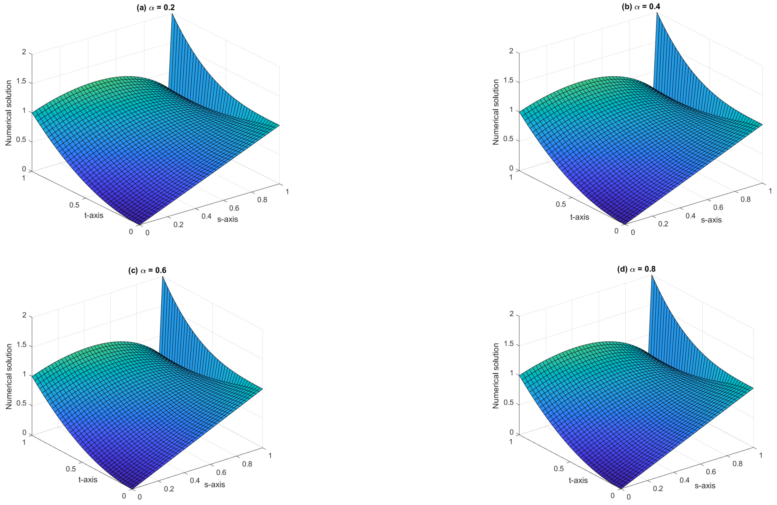
Since the analytical solution for this problem is not available, we use the double mesh principle to compute the maximum absolute error. The numerical solution for Example 2, with N = M = 40 and ϵ = 2 12 , is plotted for various values of α in Figure 2. Table 4 shows the maximum absolute errors and convergence rate for various choices of α with ϵ = 2 14 fixed. In order to illustrate ϵ uniform convergence, Table 5 displays the maximum absolute error and convergence rate for different values of N , M , and ϵ , with α = 0.5 fixed. We compare our numerical results with the results available in Sahoo [26] and tabulate them in Table 6.
Example 3 
([26]). Consider the following time-fractional SPPPDE:
D t α y ϵ 2 y s 2 + ( 2 s 2 ) y s + s y = 10 s 2 t 2 , ( s , t ) ( 0 , 1 ) × ( 0 , 1 ] ,
with
y ( s , 0 ) = s , s [ 0 , 1 ] , y ( 0 , t ) = t 2 , y ( 1 , t ) = 1 + t 3 , t [ 0 , 1 ] .
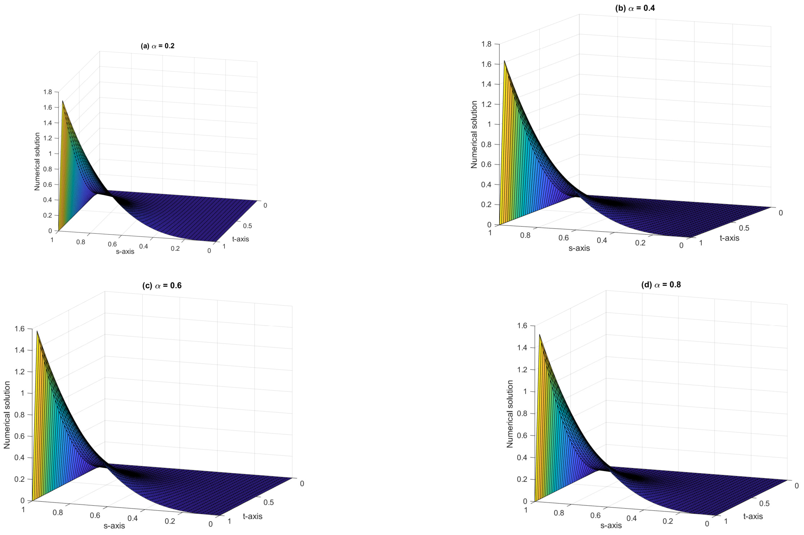
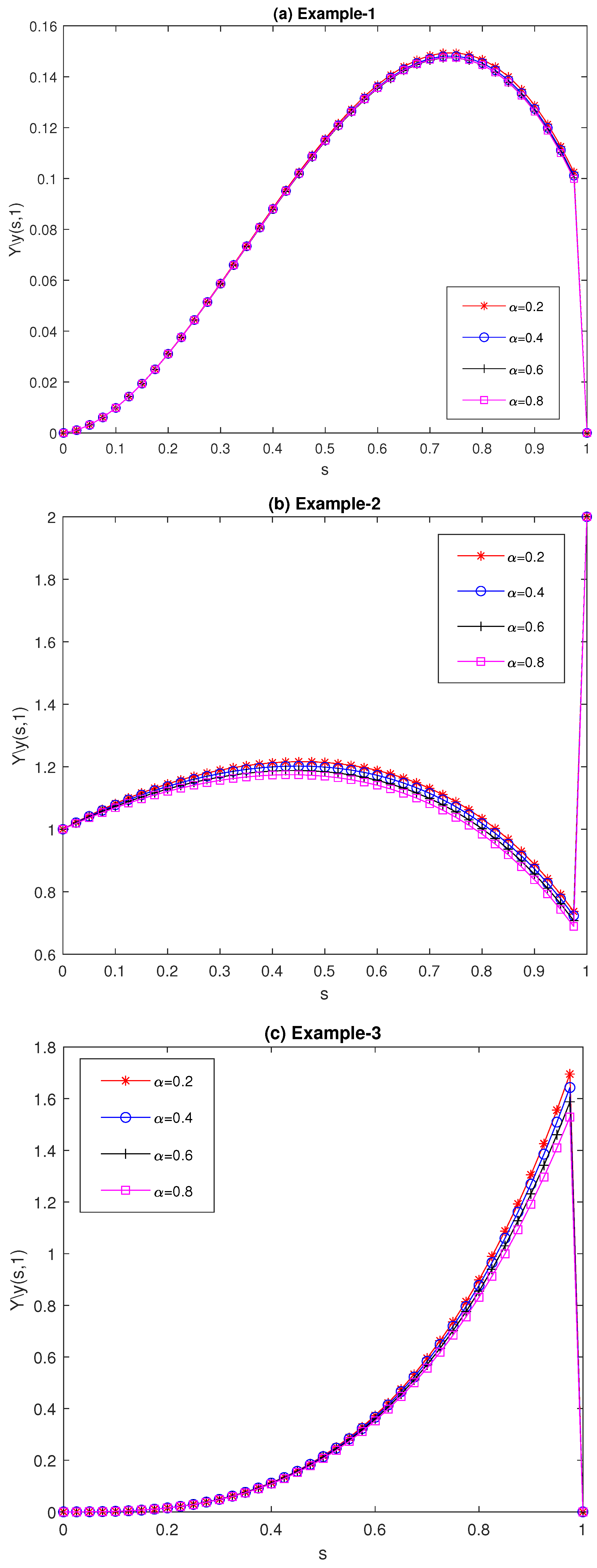
Again, the double mesh principle is employed to compute the maximum absolute error. The numerical solution for Example 3, with N = M = 40 and ϵ = 2 12 , is plotted for various values of α in Figure 3. Figure 4a, Figure 4b and Figure 4c represents the error plot for Examples 1, 2 and 3 respectively. Figure 5a, Figure 5b and Figure 5c displays the numerical findings in a line plot at the time t = 1 for various values of α . Table 7 displays the maximum absolute errors and convergence rate for various values of α with ϵ = 2 14 fixed. To demonstrate ϵ uniform convergence, Table 8 displays the maximum absolute errors and convergence rate for different values of N , M and ϵ with α = 0.5 fixed. Additionally, we compare our numerical results with those available in Sahoo [26], as shown in Table 9.

6. Conclusions

In this paper, we solve time-fractional SPPPDEs by using an NSFD scheme. The proposed approach employs the L 1 scheme for discretizing the time-fractional derivative followed by the application of the NSFD scheme for discretizing spatial derivatives on a uniform mesh. The proposed method is uniformly convergent with respect to ϵ , attaining a convergence rate of O ( N 1 + ( Δ t ) 2 α ) , providing consistent results even for very small values of ϵ . The numerical results confirm the theoretical findings, and the accuracy achieved by the proposed scheme surpasses that of existing methods in the literature. This research contributes to both the theoretical understanding and the numerical treatment of time-fractional singularly perturbed problems. The scheme is unconditionally stable and has parameter-uniform convergence. The numerical experiments demonstrate that the given method is a suitable choice for solving time-fractional SPPPDEs. A possible direction for future research is the extension of this approach to two-dimensional time-fractional singularly perturbed convection–diffusion problems.

Author Contributions

R.M.: Conceptualization, Investigation, Writing—original draft; P.C.P.: Conceptualization, Investigation, Supervision, Writing—review & editing; H.R.: Conceptualization, Investigation, Supervision, Writing—review & editing. All authors have read and agreed to the published version of the manuscript.

Funding

This research received no external funding.

Data Availability Statement

No new data were created.

Acknowledgments

The authors sincerely acknowledge the anonymous reviewers for their valuable inputs for strengthening the article.

Conflicts of Interest

The authors declare no conflicts of interest.

References

  1. Bender, C.M.; Orszag, S.A. Advanced Mathematical Methods for Scientists and Engineers, 3rd ed.; McGraw-Hill Book Co.: New York, NY, USA, 1978. [Google Scholar]
  2. Nayfeh, A.H. Introduction to Perturbation Techniques, 3rd ed.; John Wiley & Sons: New York, NY, USA, 1981. [Google Scholar]
  3. O’Malley, R.E., Jr. Introduction to Singular Perturbations, 3rd ed.; Harcourt Brace Jovanovich: New York, NY, USA, 1974. [Google Scholar]
  4. Clavero, C.; Jorge, J.C.; Lisbona, F.J. A uniformly convergent scheme on a nonuniform mesh for convection-diffusion parabolic problems. J. Comput. Appl. Math. 2003, 154, 415–429. [Google Scholar] [CrossRef]
  5. Kadalbajoo, M.K.; Gupta, V.; Awasthi, A. A uniformly convergent B-spline collocation method on a nonuniform mesh for singularly perturbed one-dimensional time-dependent linear convection-diffusion problem. J. Comput. Appl. Math. 2008, 220, 271–289. [Google Scholar] [CrossRef]
  6. Clavero, C.; Gracia, J.L.; Stynes, M. A simpler analysis of a hybrid numerical method for time-dependent convection-diffusion problems. J. Comput. Appl. Math. 2011, 235, 5240–5248. [Google Scholar] [CrossRef]
  7. Yüzbasıa, S.; Sahin, N. Numerical solutions of singularly perturbed one-dimensional parabolic convection–diffusion problems by the Bessel collocation method. Appl. Math. Comput. 2013, 220, 305–315. [Google Scholar]
  8. Clavero, C.; Gracia, J.L. A high order HODIE finite difference scheme for 1D parabolic singularly perturbed reaction-diffusion problems. Appl. Math. Comput. 2012, 218, 5067–5080. [Google Scholar] [CrossRef]
  9. Bansal, K.; Sharma, K.K. Parameter uniform numerical scheme for time dependent singularly perturbed convection-diffusion-reaction problems with general shift arguments. Numer. Algorithms 2017, 75, 113–145. [Google Scholar] [CrossRef]
  10. Chang, A.; Sun, H.G.; Zheng, C.; Lu, B.; Lu, C.; Ma, R.; Zhang, Y. A time fractional convection–diffusion equation to model gas transport through heterogeneous soil and gas reservoirs. Physica A 2018, 502, 356–369. [Google Scholar] [CrossRef]
  11. Pavlenko, I.; Ochowiak, M.; Włodarczak, S.; Krupińska, A.; Matuszak, M. Parameter identification of the fractional-Order mathematical model for convective mass transfer in a porous medium. Membranes 2023, 13, 819. [Google Scholar] [CrossRef]
  12. Podlubny, I. Fractional Differential Equations. An Introduction to Fractional Derivatives, Fractional Differential Equations, to Methods of Their Solution and Some of Their Applications; Academic Press, Inc.: San Diego, CA, USA, 1999. [Google Scholar]
  13. Kilbas, A.A.; Srivastava, H.M.; Trujillo, J.J. Theory and Applications of Fractional Differential Equations, 1st ed.; Elsevier: Amsterdam, The Netherlands, 2006; p. 523. [Google Scholar]
  14. Li, C.; Zeng, F. Numerical Methods for Fractional Calculus; CRC Press, Inc.: Boca Raton, FL, USA, 2015. [Google Scholar]
  15. Cai, M.; Li, C. Theory and Numerical Approximations of Fractional Integrals and Derivatives; Society for Industrial and Applied Mathematics: Philadelphia, PA, USA, 2020; p. 317. [Google Scholar]
  16. Lin, Y.; Xu, C. Finite difference/spectral approximations for the time-fractional diffusion equation. J. Comput. Phys. 2017, 225, 1533–1552. [Google Scholar] [CrossRef]
  17. Stynes, M.; O’Riordan, E.; Gracia, J.L. Error analysis of a finite difference method on graded meshes for a time-fractional diffusion equation. SIAM J. Numer. Anal. 2017, 55, 1057–1079. [Google Scholar] [CrossRef]
  18. Choudhary, R.; Singh, S.; Kumar, D. A second-order numerical scheme for the time-fractional partial differential equations with a time delay. Comput. Appl. Math. 2017, 41, 28. [Google Scholar] [CrossRef]
  19. Soori, Z.; Aminataei, A. A new approximation to Caputo-type fractional diffusion and advection equations on non-uniform meshes. Appl. Numer. Math. 2019, 144, 21–41. [Google Scholar] [CrossRef]
  20. Gracia, J.L.; O’Riordan, E.; Stynes, M. Convergence in positive time for a finite difference method applied to a fractional convection-diffusion problem. Comput. Methods Appl. Math. 2023, 18, 33–42. [Google Scholar] [CrossRef]
  21. Gao, G.-h.; Sun, Z.-z.; Zhang, H.-w. A new fractional numerical differentiation formula to approximate the Caputo fractional derivative and its applications. J. Comput. Phys. 2014, 259, 33–50. [Google Scholar] [CrossRef]
  22. Roul, P.; Sundar, S. Novel numerical methods based on graded, adaptive and uniform meshes for a time-fractional advection-diffusion equation subjected to weakly singular solution. Numer. Algorithms 2025, 98, 531–561. [Google Scholar] [CrossRef]
  23. Kopteva, N. Error analysis of an L2-type method on graded meshes for a fractional-order parabolic problem. Math. Comp. 2021, 90, 327. [Google Scholar] [CrossRef]
  24. Kumar, K.; P, P.C.; Vigo-Aguiar, J. Numerical solution of time-fractional singularly perturbed convection-diffusion problems with a delay in time. Math. Methods Appl. Sci. 2021, 44, 3080–3097. [Google Scholar] [CrossRef]
  25. Kumie, H.G.; Tirunehi, A.A.; Derese, G.A. Crank–Nicolson method for solving time-fractional singularly perturbed delay partial differential equations. Res. Math. 2024, 11, 2293373. [Google Scholar] [CrossRef]
  26. Sahoo, S.K.; Gupta, V. A robust uniformly convergent finite difference scheme for the time-fractional singularly perturbed convection-diffusion problem. Comput. Math. Appl. 2023, 137, 126–146. [Google Scholar] [CrossRef]
  27. Sahoo, S.K.; Gupta, V.; Dubey, S. A robust higher-order finite difference technique for a time-fractional singularly perturbed problem. Math. Comput. Simul. 2024, 215, 43–68. [Google Scholar] [CrossRef]
  28. Aniley, W.T.; Duressa, G.F. Uniformly convergent numerical method for time-fractional convection–diffusion equation with variable coefficients. Partial Differ. Equ. Appl. Math. 2023, 8, 100592. [Google Scholar] [CrossRef]
  29. Tiruneh, A.A.; Kumie, H.G.; Derese, G.A. Singularly perturbed time-fractional convection–diffusion equations via exponential fitted operator scheme. Partial Differ. Equ. Appl. Math. 2024, 11, 100873. [Google Scholar] [CrossRef]
  30. Aniley, W.T.; Duressa, G.F. A novel exponentially fitted finite-difference method for time-fractional singularly perturbed convection-diffusion problems with variable coefficients. Front. Appl. Math. Stat. 2025, 11, 1541766. [Google Scholar] [CrossRef]
  31. Caputo, M.; Fabrizio, M. On the notion of fractional derivative and applications to the hysteresis phenomena. Meccanica 2017, 52, 3043–3052. [Google Scholar] [CrossRef]
  32. Roos, H.; Stynes, M.; Tobiska, L. Robust Numerical Methods for Singularly Perturbed Differential Equations, 2nd ed.; Springer Series in Computational Mathematics; Springer: Berlin/Heidelberg, Germany, 2008. [Google Scholar]
  33. Ladyzhenskaia, O.A.; Solonnikov, V.A.; Ural’tseva, N.N. Linear and Quasi-Linear Equations of Parabolic Type, 23rd ed.; American Mathematical Society: Providence, RI, USA, 1968. [Google Scholar]
  34. Mickens, R.E. Nonstandard Finite Difference Models of Differential Equations, 3rd ed.; World Scientific Publishing Co.: River Edge, NJ, USA, 1994. [Google Scholar]
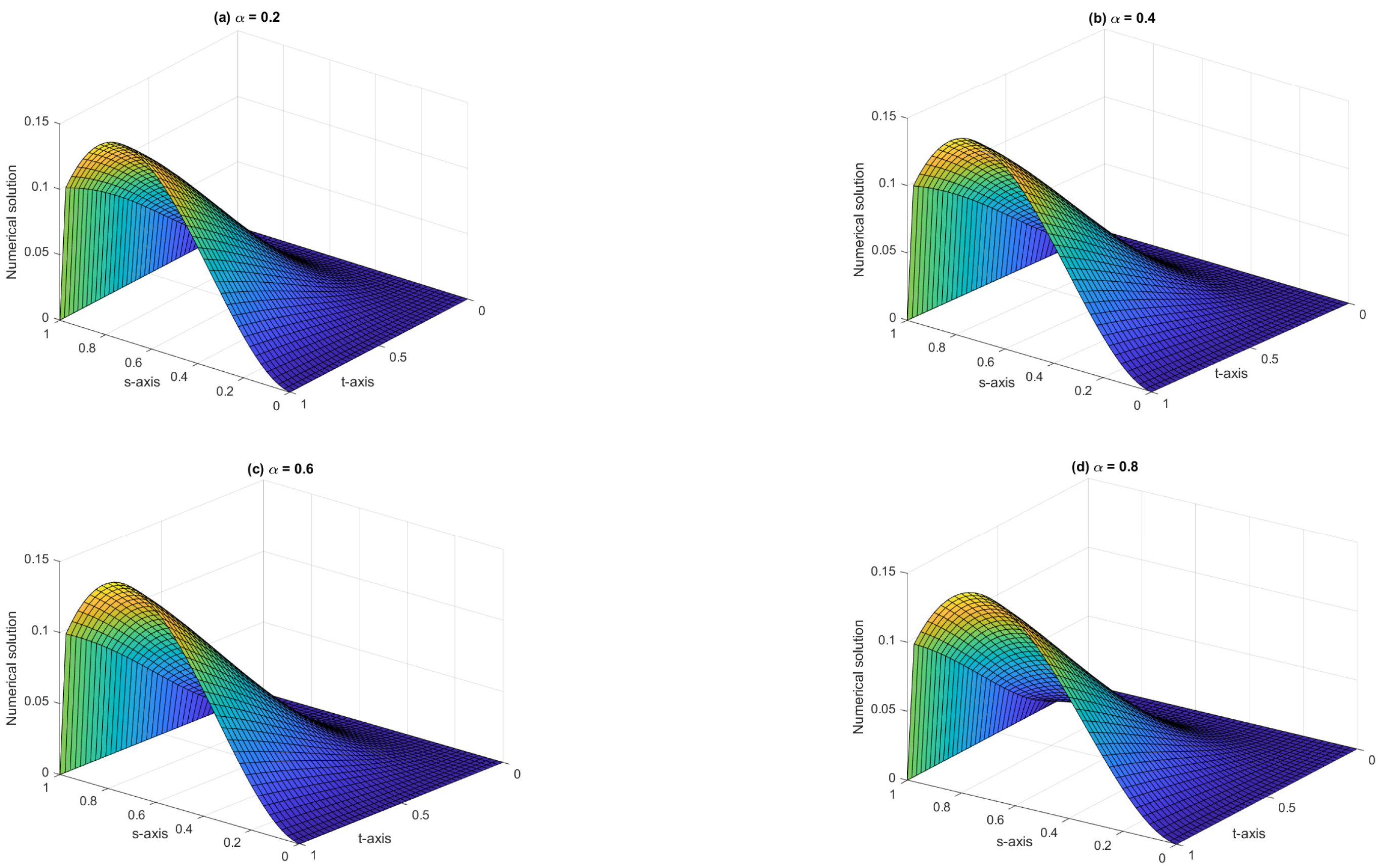
Figure 1. Graphical representation of numerical solution for Example 1, with N = M = 40 , ϵ = 2 12 and for various values of α .
Fractalfract 09 00333 g001
Figure 2. Graphical representation of numerical solution for Example 2, with N = M = 40 , ϵ = 2 12 and for various values of α .
Fractalfract 09 00333 g002
Figure 3. Graphical representation of numerical solution for Example 3, with N = M = 40 and ϵ = 2 12 and for various values of α .
Fractalfract 09 00333 g003
Figure 4. Error plots for Examples 1–3 are presented in graphs (a), (b), and (c), respectively, when α = 0.5 .
Fractalfract 09 00333 g004
Figure 5. Line plots for Examples 1–3 for different values of α are presented in graphs (a), (b), and (c), respectivly, when ϵ = 2 12 .
Fractalfract 09 00333 g005
Table 1. Maximum errors and convergence rate for Example 1, with ϵ = 2 14 and for various values of α .
N , M α = 0.25   α = 0.50   α = 0.75  
ErRocErRocErRoc
32 , 32 2.5135 × 10 3 0.9291 2.5006 × 10 3 0.9320 2.5645 × 10 3 0.9344
64 , 64 1.3201 × 10 3 0.9654 1.3106 × 10 3 0.9675 1.3418 × 10 3 0.9700
128 , 128 6.7604 × 10 4 0.9829 6.7021 × 10 4 0.9844 6.8501 × 10 4 0.9869
256 , 256 3.4203 × 10 4 3.3873 × 10 4 3.4562 × 10 4
Table 2. Maximum errors and convergence rate for Example 1, with α = 0.5 fixed and for various values of N , M and ϵ .
ϵ N = 20 N = 40 N = 80 N = 160 N = 320
M = 20M = 40M = 80M = 160M = 320
2 6 2.6646 × 10 3 8.3968 × 10 4 2.4325 × 10 4 6.3551 × 10 5 1.6055 × 10 5
  1.6660 1.7874 1.9365 1.9849 -
2 7 3.6173 × 10 3 1.4750 × 10 3 4.5494 × 10 4 1.2358 × 10 4 3.2173 × 10 5
  1.2941 1.6970 1.8803 1.9415 -
2 8 3.7683 × 10 3 1.9472 × 10 3 7.7745 × 10 4 2.3707 × 10 4 6.3027 × 10 5
  0.95254 1.3246 1.7135 1.9112 -
2 9 3.7714 × 10 3 2.0370 × 10 3 1.0077 × 10 3 3.9768 × 10 4 1.2079 × 10 4
  0.8886 1.0154 1.3414 1.7191 -
2 10 3.7714 × 10 3 2.0390 × 10 3 1.0569 × 10 3 5.1210 × 10 4 2.0146 × 10 4
  0.8872 0.9480 1.0453 1.3459 -
2 11 3.7714 × 10 3 2.0390 × 10 3 1.0581 × 10 3 5.3789 × 10 4 2.5866 × 10 4
  0.8872 0.9464 0.9760 1.0563 -
2 12 3.7714 × 10 3 2.0390 × 10 3 1.0581 × 10 3 5.3851 × 10 4 2.7122 × 10 4
  0.8872 0.9464 0.9743 0.9895 -
2 13 3.7714 × 10 3 2.0390 × 10 3 1.0581 × 10 3 5.3851 × 10 4 2.7155 × 10 4
  0.8872 0.9464 0.9743 0.9877 -
2 14 3.7714 × 10 3 2.0390 × 10 3 1.0581 × 10 3 5.3851 × 10 4 2.7155 × 10 4
  0.8872 0.9464 0.9743 0.9877 -
2 28 3.7714 × 10 3 2.0390 × 10 3 1.0581 × 10 3 5.3851 × 10 4 2.7155 × 10 4
  0.8872 0.9464 0.9743 0.9877 -
2 30 3.7714 × 10 3 2.0390 × 10 3 1.0581 × 10 3 5.3851 × 10 4 2.7155 × 10 4
  0.8872 0.9464 0.9743 0.9877 -
Table 3. Comparision of computed solution with Sahoo [26] for Example 1, with α = 0.4 and for various values of N , M and ϵ .
 Sahoo [26]Present MethodSahoo [26]Present Method
ϵ /(N,M) (32, 32)(32, 32)(64, 64)(64, 64)
10 2 6.4038 × 10 3 1.7602 × 10 3 3.4049 × 10 3 5.4366 × 10 4
10 3 7.0384 × 10 3 2.4994 × 10 3 3.9629 × 10 3 1.3109 × 10 3
10 4 7.0667 × 10 3 2.4994 × 10 3 3.9905 × 10 3 1.3112 × 10 3
10 5 7.0687 × 10 3 2.4994 × 10 3 3.9921 × 10 3 1.3112 × 10 3
10 10 7.0689 × 10 3 2.4994 × 10 3 3.9922 × 10 3 1.3112 × 10 3
Table 4. Maximum errors and convergence rate for Example 2, with ϵ = 2 14 and for various values of α .
N , M α = 0.25   α = 0.50   α = 0.75  
ErRocErRocErRoc
32 , 32 1.1921 × 10 2 0.9454 1.1507 × 10 2 0.9413 1.0978 × 10 2 0.9342
64 , 64 6.1898 × 10 3 0.9723 5.9926 × 10 3 0.9696 5.7453 × 10 3 0.9641
128 , 128 3.1547 × 10 3 0.9860 3.0601 × 10 3 0.9841 2.9449 × 10 3 0.9796
256 , 256 1.5927 × 10 3 1.5469 × 10 3 1.4934 × 10 3
Table 5. Maximum errors and convergence rate for Example 2, with α = 0.5 fixed and for various values of N , M and ϵ .
ϵ N = 20 N = 40 N = 80 N = 160 N = 320
M = 20M = 40M = 80M = 160M = 320
2 6 1.7139 × 10 2 8.1080 × 10 3 2.7622 × 10 3 7.3455 × 10 4 1.8594 × 10 4
  1.0799 1.5535 1.9109 1.9820 -
2 7 1.7545 × 10 2 9.1309 × 10 3 4.2143 × 10 3 1.4125 × 10 3 3.7514 × 10 4
  0.9422 1.1155 1.5770 1.9127 -
2 8 1.7556 × 10 2 9.3482 × 10 3 4.7188 × 10 3 2.1510 × 10 3 7.1486 × 10 4
  0.9092 0.9862 1.1334 1.5892 -
2 9 1.7556 × 10 2 9.3556 × 10 3 4.8300 × 10 3 2.4004 × 10 3 1.0873 × 10 3
  0.9080 0.9538 1.0087 1.1426 -
2 10 1.7556 × 10 2 9.3556 × 10 3 4.8342 × 10 3 2.4564 × 10 3 1.2111 × 10 3
  0.9080 0.9525 0.9767 1.0202 -
2 11 1.7556 × 10 2 9.3556 × 10 3 4.8342 × 10 3 2.4587 × 10 3 1.2392 × 10 3
  0.9080 0.9525 0.9753 0.9884 -
2 12 1.7556 × 10 2 9.3556 × 10 3 4.8342 × 10 3 2.4587 × 10 3 1.2404 × 10 3
  0.9080 0.9525 0.9753 0.9871 -
2 13 1.7556 × 10 2 9.3556 × 10 3 4.8342 × 10 3 2.4587 × 10 3 1.2404 × 10 3
  0.9080 0.9525 0.9753 0.9871 -
2 14 1.7556 × 10 2 9.3556 × 10 3 4.8342 × 10 3 2.4587 × 10 3 1.2404 × 10 3
  0.9080 0.9525 0.9753 0.9871 -
2 28 1.7556 × 10 2 9.3556 × 10 3 4.8342 × 10 3 2.4587 × 10 3 1.2404 × 10 3
  0.9080 0.9525 0.9753 0.9871 -
2 30 1.7556 × 10 2 9.3556 × 10 3 4.8342 × 10 3 2.4587 × 10 3 1.2404 × 10 3
  0.9080 0.9525 0.9753 0.9871 -
Table 6. Comparision of computed solution in Sahoo [26] for Example 2, with α = 0.4 and for various values of N , M and ϵ .
 Sahoo [26]Present MethodSahoo [26]Present Method
ϵ /(N,M) (32, 32)(32, 32)(64, 64)(64, 64)
10 2 2.6796 × 10 2 1.1381 × 10 2 1.4684 × 10 2 5.2547 × 10 3
10 3 2.8892 × 10 2 1.1677 × 10 2 1.5554 × 10 2 6.0721 × 10 3
10 4 2.9451 × 10 2 1.1677 × 10 2 1.6018 × 10 2 6.0721 × 10 3
10 5 2.9509 × 10 2 1.1677 × 10 2 1.6081 × 10 2 6.0721 × 10 3
10 10 2.9516 × 10 2 1.1677 × 10 2 1.6088 × 10 2 6.0721 × 10 3
Table 7. Maximum errors and convergence rate for Example 3, with ϵ = 2 14 and for various values of α .
N , M α = 0.25   α = 0.50   α = 0.75  
ErRocErRocErRoc
32 , 32 2.8710 × 10 2 0.9460 2.5751 × 10 2 0.9535 2.3194 × 10 2 0.9676
64 , 64 1.4902 × 10 2 0.9730 1.3296 × 10 2 0.9780 1.1860 × 10 2 0.9889
128 , 128 7.5915 × 10 3 0.9866 6.7500 × 10 3 0.9900 5.9756 × 10 3 0.9989
256 , 256 3.8311 × 10 3 3.3983 × 10 3 2.9900 × 10 3
Table 8. Maximum errors and convergence rate for Example 3, with α = 0.5 fixed and for various values of N , M and ϵ .
ϵ N = 20 N = 40 N = 80 N = 160 N = 320
M = 20M = 40M = 80M = 160M = 320
2 6 3.3299 × 10 2 1.0905 × 10 2 2.9887 × 10 3 7.7438 × 10 4 1.9825 × 10 4
  1.6105 1.8674 1.9484 1.9657 -
2 7 3.8686 × 10 2 1.7523 × 10 2 5.5582 × 10 3 1.5331 × 10 3 3.9463 × 10 4
  1.1426 1.6565 1.8582 1.9579 -
2 8 3.9578 × 10 2 2.0363 × 10 2 8.9798 × 10 3 2.8213 × 10 3 7.7459 × 10 4
  0.9587 1.1812 1.6703 1.8649 -
2 9 3.9599 × 10 2 2.0857 × 10 2 1.0437 × 10 2 4.5415 × 10 3 1.4214 × 10 3
  0.9249 0.9988 1.2005 1.6758 -
2 10 3.9599 × 10 2 2.0871 × 10 2 1.0695 × 10 2 5.2790 × 10 3 2.2821 × 10 3
  0.9240 0.9644 1.0186 1.2099 -
2 11 3.9599 × 10 2 2.0871 × 10 2 1.0703 × 10 2 5.4112 × 10 3 2.6531 × 10 3
  0.9240 0.9634 0.9840 1.0283 -
2 12 3.9599 × 10 2 2.0871 × 10 2 1.0703 × 10 2 5.4154 × 10 3 2.7198 × 10 3
  0.9240 0.9634 0.9829 0.9935 -
2 13 3.9599 × 10 2 2.0871 × 10 2 1.0703 × 10 2 5.4154 × 10 3 2.7220 × 10 3
  0.9240 0.9634 0.9829 0.9923 -
2 14 3.9599 × 10 2 2.0871 × 10 2 1.0703 × 10 2 5.4154 × 10 3 2.7220 × 10 3
  0.9240 0.9634 0.9829 0.9923 -
2 28 3.9599 × 10 2 2.0871 × 10 2 1.0703 × 10 2 5.4154 × 10 3 2.7220 × 10 3
  0.9240 0.9634 0.9829 0.9923 -
2 30 3.9599 × 10 2 2.0871 × 10 2 1.0703 × 10 2 5.4154 × 10 3 2.7220 × 10 3
  0.9240 0.9634 0.9829 0.9923 -
Table 9. Comparision of computed solution with Sahoo [26] for Example 3, with α = 0.4 and for various values of N , M and ϵ .
 Sahoo [26]Present MethodSahoo [26]Present Method
ϵ /(N,M) (32, 32)(32, 32)(64, 64)(64, 64)
10 2 3.8542 × 10 2 2.2317 × 10 2 2.0585 × 10 2 7.0169 × 10 3
10 3 4.4131 × 10 2 2.6920 × 10 2 2.3663 × 10 2 1.3934 × 10 2
10 4 4.6471 × 10 2 2.6920 × 10 2 2.4571 × 10 2 1.3936 × 10 2
10 5 4.6726 × 10 2 2.6920 × 10 2 2.4854 × 10 2 1.3936 × 10 2
10 10 4.6755 × 10 2 2.6920 × 10 2 2.4886 × 10 2 1.3936 × 10 2
Disclaimer/Publisher’s Note: The statements, opinions and data contained in all publications are solely those of the individual author(s) and contributor(s) and not of MDPI and/or the editor(s). MDPI and/or the editor(s) disclaim responsibility for any injury to people or property resulting from any ideas, methods, instructions or products referred to in the content.