1. Introduction
Fractional calculus [
1,
2] generalizes classical calculus by introducing derivatives and integrals of non-integer (and even complex) order. Unlike traditional differential operators, which are restricted to integer orders, fractional operators enable continuous-order differentiation and integration, providing a powerful framework for modeling memory-dependent and nonlocal phenomena. A major impetus for fractional calculus arises from the study of anomalous diffusion, where particle spreading deviates from classical Brownian motion. Instead of the mean squared displacement growing linearly with time (as in Fickian diffusion), anomalous diffusion exhibits power-law scaling. Such processes are naturally described by fractional differential equations, wherein the classical time derivative is replaced with a fractional counterpart—such as the Caputo or Riemann–Liouville derivative. Solutions to fractional differential equations frequently involve Mittag–Leffler functions, which generalize the exponential function and are essential for capturing power-law decay and memory effects. These functions are particularly crucial in modeling non-Debye relaxation in disordered materials [
3] (e.g., glasses and amorphous solids), where traditional exponential decay fails to describe observed dynamics. Their asymptotic behavior accurately reproduces the stretched exponential relaxation seen in dielectric spectroscopy and mechanical responses. In soft matter systems—such as polymer networks, gels, and biological tissues—Mittag–Leffler functions emerge naturally within fractional viscoelastic models [
4] due to power-law memory kernels. However, analytical solutions for fractional differential equations are often intractable, necessitating robust numerical approximation methods. Among these, Grünwald–Letnikov approximation [
5,
6] has become a widely adopted approach due to its straightforward implementation and theoretical consistency with the fractional calculus framework.
Impulse control is a regulatory mechanism that governs system states through the application of instantaneous perturbations at discrete-time points, thereby conferring a distinct set of advantages for fractional order discrete systems. It is evident that such systems manifest more intricate dynamics than integer-order systems due to their memory effects and nonlocal characteristics. Consequently, this renders traditional continuous control less efficient. The application of control is restricted to specific moments, thereby reducing the computational burden and energy consumption while effectively managing chaotic behavior. It is imperative that these controllers exhibit sufficient robustness against parameter uncertainties, encompassing system dynamics, control gains, and timing accuracy, to ensure stability under disturbances. Lyapunov-based methods ensure this stability by enforcing energy dissipation during impulsive phases.
Given these advantages, impulsive controlling techniques are robust in stability studies because they only require a small control gain working at isolated time points and the implementation cost could be decreased. With these benefits, there exist numerous stability analyses of discrete-time and continuous-time systems by means of impulsive controls. For instance, Miaadi and Li [
7] discussed finite time stabilization and synchronization of neural networks by using impulsive techniques. The authors [
8,
9] investigated the input-to-state stability of nonlinear continuous-time systems via impulsive controls. Alluding to the discrete-time case, papers [
10,
11,
12] discussed the stability of some Markovian jump or stochastic discrete-time systems with impulsive effects. For the nonlocal continuous-time case, Zhang et al. [
13] employed the pulse impacts to stabilize fractional order neural networks. The synchronization issues of impulsive fractional order bidirectional associative memory neural networks were the focal point of the authors’ research [
14]. For the nonlocal discrete-time case, studies [
15,
16] addressed the stability or synchronization to several kinds of nonlocal discrete-time models. In addition, this method proves especially valuable for Chua’s oscillator [
17,
18], whose fractional order discrete form exhibits enhanced chaotic behavior. Strategically designed impulsive interventions not only stabilize the system but also exploit its memory effects to prolong control influence. Potential applications include secure communication and neural networks, where responsiveness and energy efficiency are paramount.
As everyone knows, control methodologies proposed for discrete-time models could be achieved more efficiently in practical systems [
19,
20,
21,
22]. Despite there being numerous studies on nonlocal continuous-time systems, there have been very few studies on nonlocal discrete-time systems until recently. During the past decades, nevertheless, a surge of discrete configurations for nonlocal calculus were proposed and developed in studies of nonlocal discrete-time systems. These works implied that the studies of nonlocal discrete-time systems have massive unexpected difficulties and technical complications. For instance, Samko et al. [
23] put forward a Grünwald–Letnikov-like operator and it has been applied widely in research into the engineering area. The authors in ref. [
24] introduced on their own the basic delta and nabla nonlocal discrete-time systems, which were diffusely discussed during these years, see [
25]. Meanwhile, the delta and nabla nonlocal discrete-time systems with
h-differences were described in ref. [
26]. The other types of nonlocal discrete-time systems could be read in studies [
27,
28,
29].
Remarkably, very few studies are concerned with the researches of nonlocal discrete-time systems with impulsive controls. In accordance with Mittag–Leffler Euler differences for nonlocal differential equations with short memory, a piecewise nonlocal discrete-time system involving Mittag–Leffler kernels is modelled for the first time. Next, an instantaneously impulsive controller is designed to exponentially stabilize this type of discrete-time oscillator. The work in this paper not only complements the existing results for the investigations of impulsive controls to nonlocal discrete-time systems in refs. [
15,
16], but also provides a new approach to discuss the dynamics of nonlocal discrete-time systems, which are different from those in refs. [
15,
16,
24,
28,
29].
1.1. Related Works
For impulsive controls to integer order nonlinear discrete-time systems with time interval and instantaneously impulsive controls, the readers should refer to papers [
11,
12,
15,
16,
30,
31,
32].
Time interval impulsive controls. In papers [
10,
11,
12,
30,
31], the authors discussed the following time interval impulsive controlled nonlinear discrete-time system
where
for some
a,
h, which is positive, shows the timing step,
,
stands for some nonlinear function,
denotes the pulse function. Fang et al. [
30] investigated the stabilization of Equation (
1). Papers [
10,
11,
12] considered the (exponential) stability of Equation (
1) with Markov jumps or stochastic distributions by means of the Lyapunov functional method, the discrete average impulsive interval approach, and the Razumikhin technique. Dai et al. [
31] studied the exponential attracting sets to Equation (
1) with Markovian jumps and stochastic disturbances via the Lyapunov–Razumikhin technique.
Instantaneously impulsive controls. In papers [
15,
16,
32], the authors focused on the following instantaneously impulsive controlled nonlinear discrete-time system
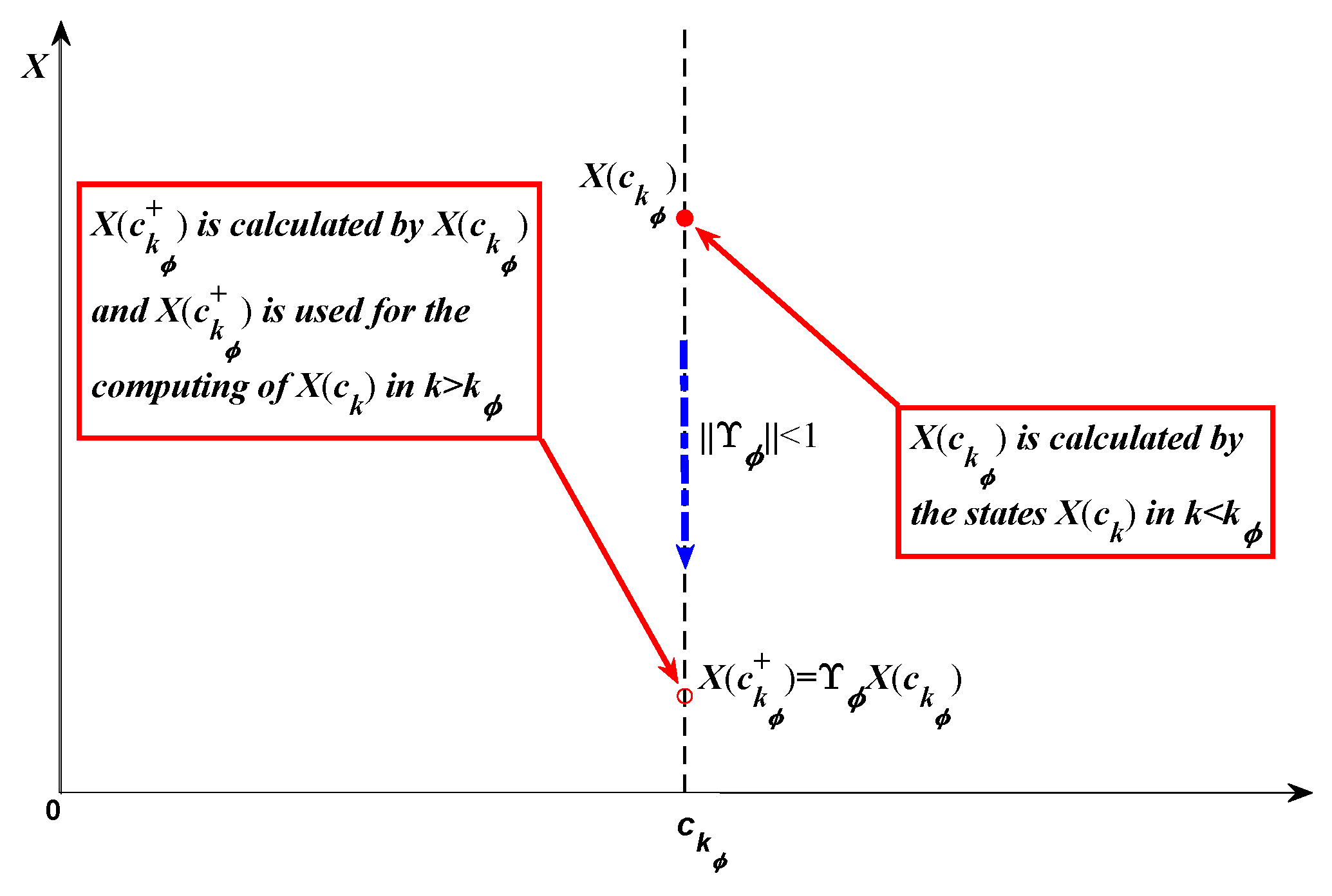
where
represents the value of
X at time
after the pulse action (here supposing the pulse action time is 0), see
Figure 1. Ref. [
32] studied input-to-state stability for Equation (
2) with switched and delayed effects via the Lyapunov–Krasovskii functional method.
For impulsive controls to nonlocal nonlinear discrete-time systems with instantaneously impulsive controls, the authors [
15,
16] investigated
where
denotes the fractional difference operator defined in papers [
15,
16]. Li and Kao in paper [
15] studied synchronous stability for a fractional order discrete-time dynamical network system based on Equation (
3). Megherbi et al. in paper [
16] discussed impulsive synchronization of chaotic systems based on Equation (
3). For more results on impulsive controlled discrete-time systems, please refer to papers [
33,
34,
35].
1.2. Novelties and Aims of This Paper
Consider the continuous-time nonlinear system with short memory as below
where
,
,
,
stands for Caputo nonlocal derivative of
u, which is defined by
where
for
.
Based on the Mittag–Leffler Euler difference to Equation (
4), a novel nonlocal difference operator is introduced and the first aim of this paper is to formulate a piecewise nonlocal discrete-time model, which can be described by
where
is a nonlocal piecewise difference operator defined later;
,
and
represent the starting point, time step size and the order of nonlocal difference, respectively;
is a parameter. Next, we discuss a piecewise nonlocal discrete-time oscillator with impulses and an instantaneously impulsive controller is designed perfectly. Finally, the proposed idea and method are employed to study piecewise nonlocal Chua’s oscillator. This paper introduces several novelties that will be discussed in greater detail in subsequent sections.
- (1)
A novel piecewise nonlocal difference operator is introduced that differs from those previously described in published papers [
15,
16,
24,
28,
29] on the subject.
- (2)
The proposed difference operator allows the formulation of a piecewise nonlocal discrete-time system. In comparison with previous studies [
23,
24,
25,
26,
27], this approach offers a variation-of-constants formula that facilitates the study and calculation of the system in practical applications.
- (3)
The design of an instantaneously impulsive controller is presented, which is intended to exponentially stabilize piecewise nonlocal discrete-time oscillators. Furthermore, a corresponding algorithm is established, which can be realized.
- (4)
The acquired control algorithm is applied in the context of the impulsive stabilization challenge associated with the Chua’s oscillator.
1.3. Plan of This Paper and Symbols
Section 2 newly introduces a piecewise nonlocal discrete-time oscillator with Mittag–Leffler kernels (MLKs) via Mittag–Leffler Euler differences. An instantaneously impulsive controller and the realizable algorithm are designed for such a nonlocal discrete-time oscillator with MLKs in
Section 3. As an application, the acquired approach was applied to the study of impulsive stabilization of nonlocal discrete-time Chua’s oscillator in
Section 4. The final section of this article presents the conclusions and perspectives derived from its content.
2. Piecewise Nonlocal Discrete-Time Oscillator
Numerous difference methods in exponential form were proposed in refs. [
19,
20] for integer order differential systems. For nonlocal differential equations, exponential Euler difference methods were similarly introduced in papers [
19,
36,
37]. Here, they are called Mittag–Leffler Euler differences since they are involved in Mittag–Leffler functions. The predecessors [
36,
37] discussed some good properties of Mittag–Leffler Euler differences. According to the Mittag–Leffler Euler difference of Equation (
4), this section will formulate a piecewise nonlocal difference equation for the first time.
2.1. Mittag–Leffler Euler Difference
Set
and
for some
. Choosing a suitable set
ensures that
satisfies
where
is a predetermined constant if
; otherwise,
, which denotes the step size from starting point
,
. The relations of sequences
,
, and
can be understood clearly in
Figure 2.
According to the difference method in ref, [
36], the Mittag–Leffler Euler difference form of Equation (
4) is given by
where
,
,
,
,
where
. Hereby,
With no need for any verifications, the parameters in Equation (
6) admit the following properties.
- (K1)
for , .
- (K2)
for all .
- (K3)
for and for , .
- (K4)
for , .
- (K5)
, .
- (K6)
.
- (K7)
If , then , and .
- (K8)
If , then is finite as .
- (K9)
Taking
for some
. If
, then
for all
,
.
Remark 1. This study is mainly devoted to discussing the piecewise model. The piecewise trait enables us to easily estimate the bounds of the chief parameters in Equation (6) by (K3) and (K6)–(K8). It should be noted that the bounds of these parameters are crucial to the discussions of the global solution, exponential stability, and controllability for nonlinear oscillators. Observing the old investigations of nonlocal discrete-time systems in refs. [15,16,23,24,25,26,27], it is hard to calculate the bounds of systematic parameters and so almost no research considers the issues of nonlocal discrete-time systems such as the existence of a unique global solution and synchronization, etc. However, Equation (6) is capable of studying these problems. 2.2. Piecewise Nonlocal Difference Equation
For the above notations, there are some indetectable relations as below.
- (T1)
if , .
- (T2)
if , .
- (T3)
and if , .
- (T4)
if and , .
- (T5)
if , .
By (T1)–(T5), Equation (
6) becomes
where
.
Denote
and
the collections of the whole functions
and
, respectively. Let
be expressed as
So,
is a linear operator and possesses a unique inverse mapping
, which is computed by
where
.
In accordance with
and
, Equation (
7) can be reformulated by
which yields
Note that Equation (
8) is equal to the Mittag–Leffler Euler difference form Equation (
6) of Equation (
4). Therefore, the Mittag–Leffler Euler
-difference could be well defined as follows.
Definition 1. The Mittag–Leffler Euler Δ-difference of with order , lower limit and parameter is given by Note that (
9) possesses piecewise feature and variable step length
in each segment
,
. It has an equivalent piecewise form given by
where
In the above calculations,
where
,
.
Remark 2 (Long memory). Take for some , . Then, and in (9), . At the moment, (9) has no piecewise trait, which can be described as Remark 3 (Exponential Euler differences). If in Remark 2, thenwhere . in (10) is called the exponential Euler Δ-difference, which has been extensively discussed in refs. [19,20]. Let
. Then,
and
,
. Obviously,
for
,
. Furthermore,
could be computed successively by
for
Based on Definition 1, some properties are listed as below. Hereby, and .
Property 1. The Mittag–Leffler Euler difference of the continuous-time system is given by nonlocal difference Equation (5). Property 2. for , .
Proof. Let
,
. It calculates
and
which implies that
for
.
If
, then it results in
Correspondingly,
and
which implies that
for
.
By the mathematical induction, , . Similarly, it easily obtains , . The proof is ended. □
Property 3. Let and . Then The derivations of Properties 1, 3, and 4 are simple and we omit the detailed proofs.
By Definition 1, Equation (
6) is reformulated by the nonlocal discrete-time oscillator with MLKs:
Let
; Equation (
11) is changed into
Equation (
11) is equal to
If
, Equation (
12) is turned into
Remark 4. The form of Equation (13) is consistent with variation-of-constants formulas studied in papers [19,20]. So Equation (12) is an expansion of the corresponding results in papers [19,20]. Compared with the previous nonlocal discrete-time systems in refs. [23,24,25,26,27], the variation-of-constants formulas in Equation (12) are easier to study and calculate in practical applications. As everyone knows, a variation-of-constants formula plays an important role in the discussion of semi-linear problems depicted by ordinary differential or difference equations, particularly in the existence and uniqueness of various solutions, stability, and other control issues. Until now, several variation-of-constants formulas for nonlocal discrete-time systems had been proposed involving various discrete Mittag–Leffler functions. For example, refs. [28,29] discussed a delta nonlocal discrete-time system:where denotes the delta Caputo fractional difference defined in Definition 13 of [28], , , , , . A variation-of-constants formula for Equation (14) was introduced in [28,29] as belowwhere E is the discrete Mittag–Leffler function defined bywhere , and for and . Obviously, the values of the kernel functions and () of Equation (12) are mainly dependent on continuous Mittag–Leffler functions. Some fine properties of continuous Mittag–Leffler functions can be used to discuss Equation (12). Meanwhile, many properties of discrete Mittag–Leffler function in Equation (15) still need to be further researched and some properties of continuous Mittag–Leffler functions may not be valid for discrete Mittag–Leffler functions. For instance, the continuous Mittag–Leffler function is convergent for , but in Equation (15) needs a strict condition to guarantee its convergence in the discussions in ref. [29]. These reasons cause the variation-of-constants formulas in [28,29] to have more difficulty than Equation (12) in the studies of nonlocal discrete-time systems. 4. Nonlocal Chua’s Oscillator
Chua’s model is a simple electronic model, which displays abundant nonlinear dynamical behaviors such as chaos and bifurcation, etc. The mathematical structure of Chua’s model has been frequently discussed with fractional order derivatives by some scholars [
38,
39,
40]. In a general way, the dynamical model of Chua’s circuit with piecewise Caputo nonlocal derivatives could be depicted by
where
,
,
,
,
are the controlled parameters of the system. The parameters’ values of Chua’s model Equation (
23) are taken from [
38]:
,
,
,
,
,
.
Let
,
,
,
and
. The numerical solution of Equation (
23) can be depicted by a nonlocal discrete-time oscillator as below
where
,
, and
. By numerical simulations with
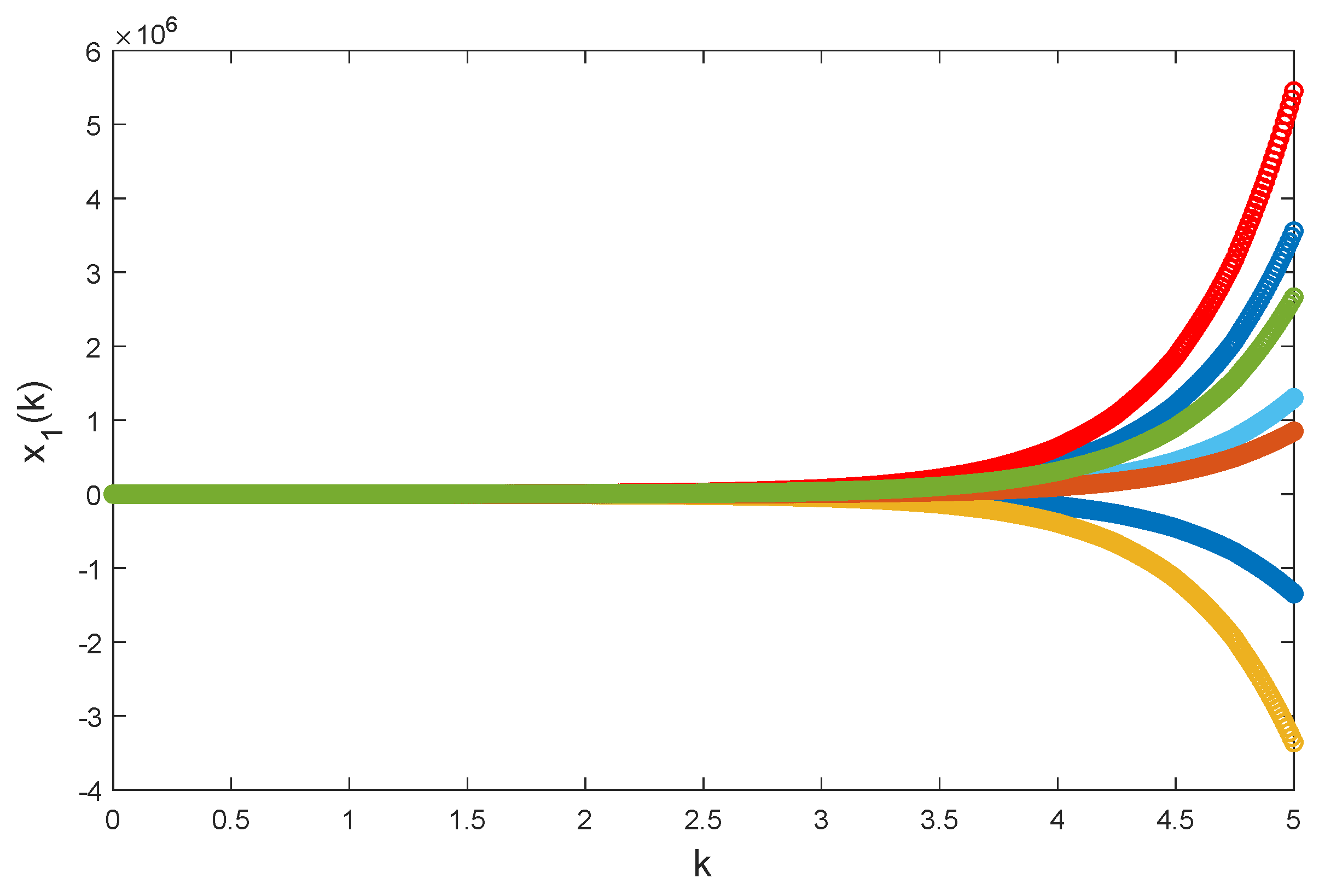
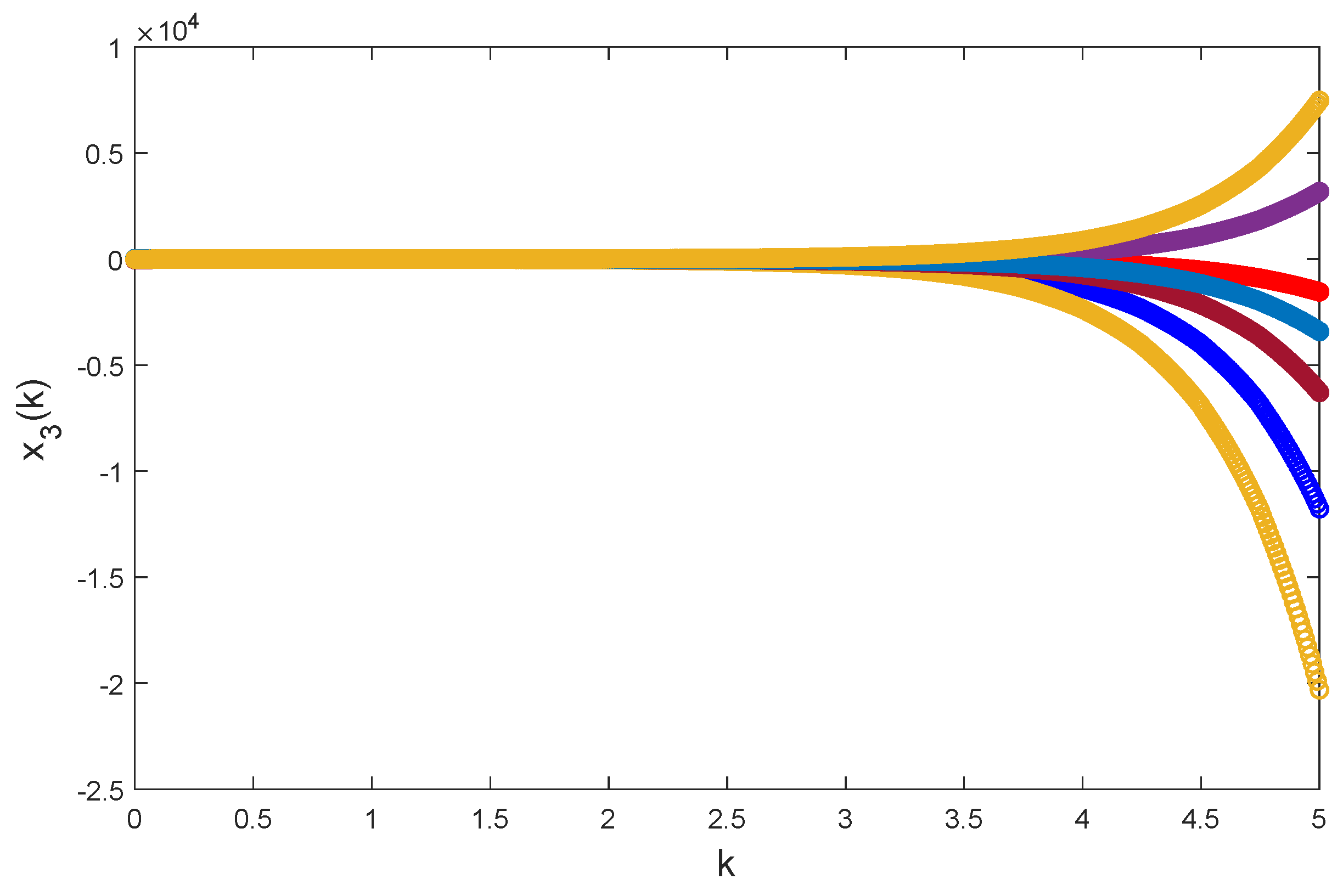
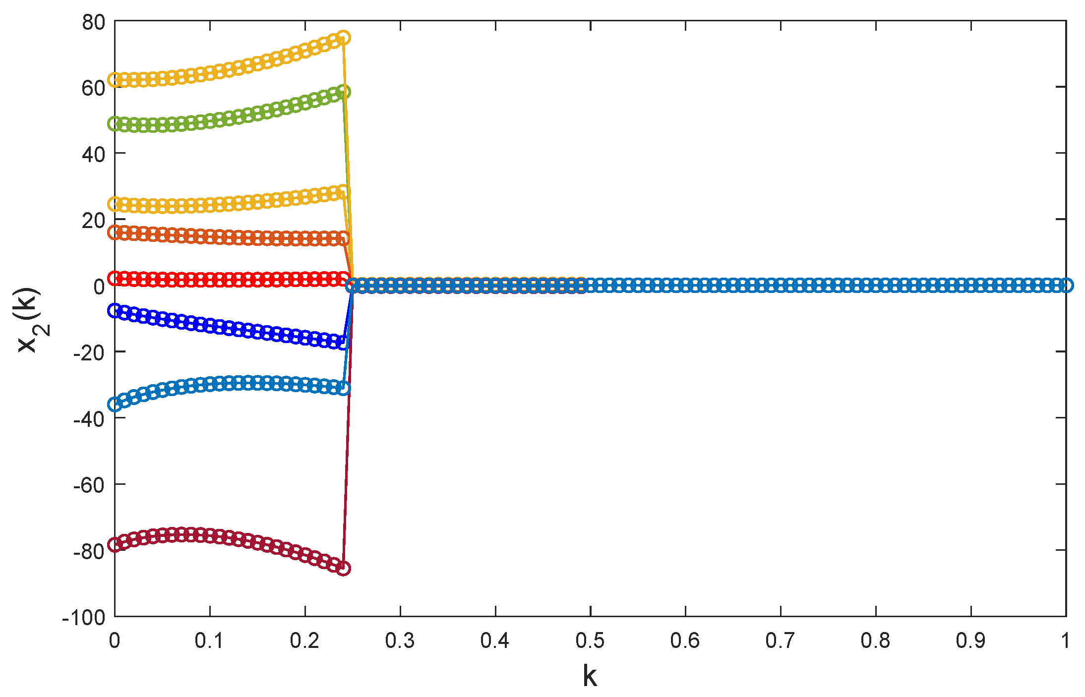
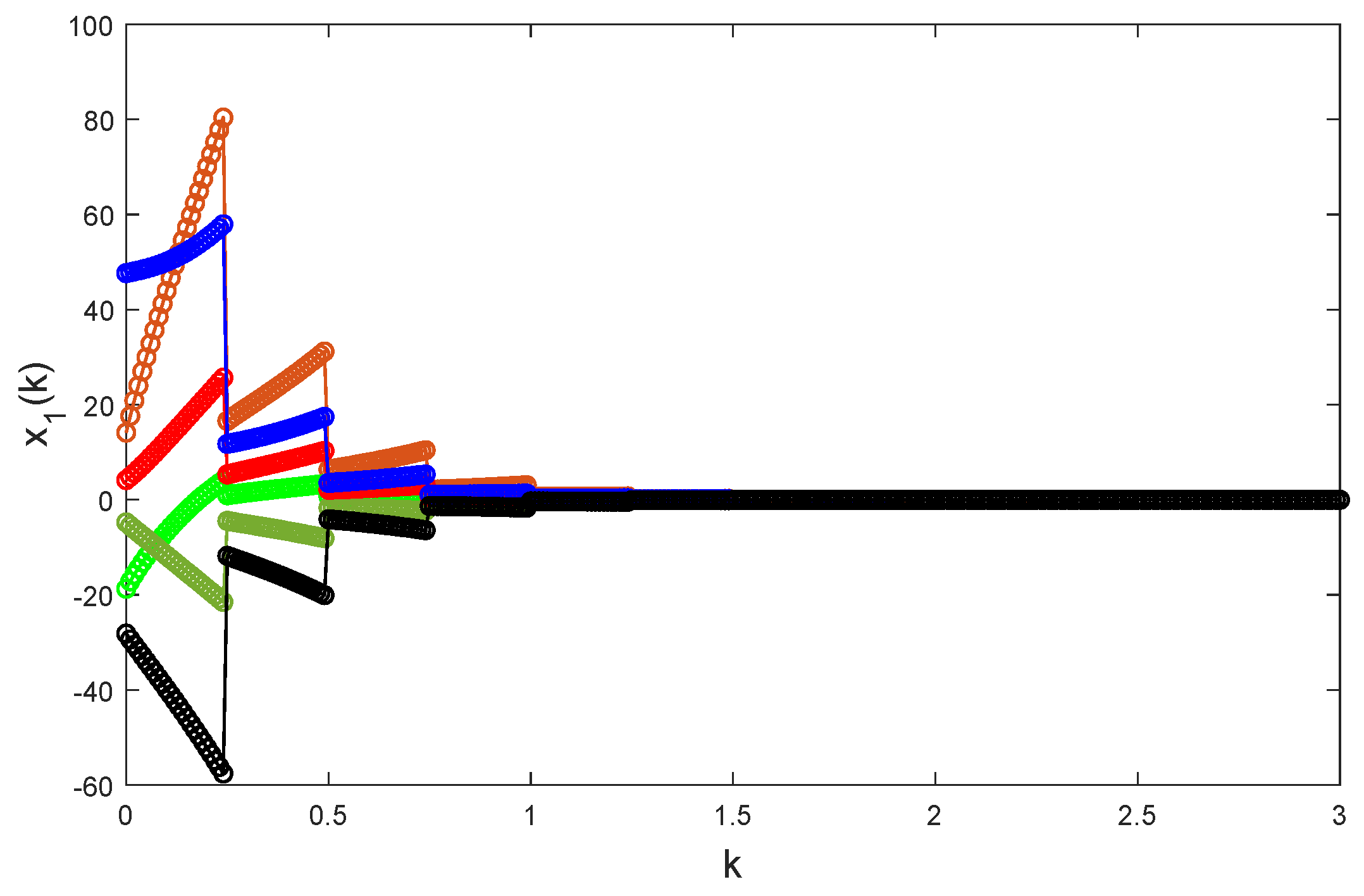
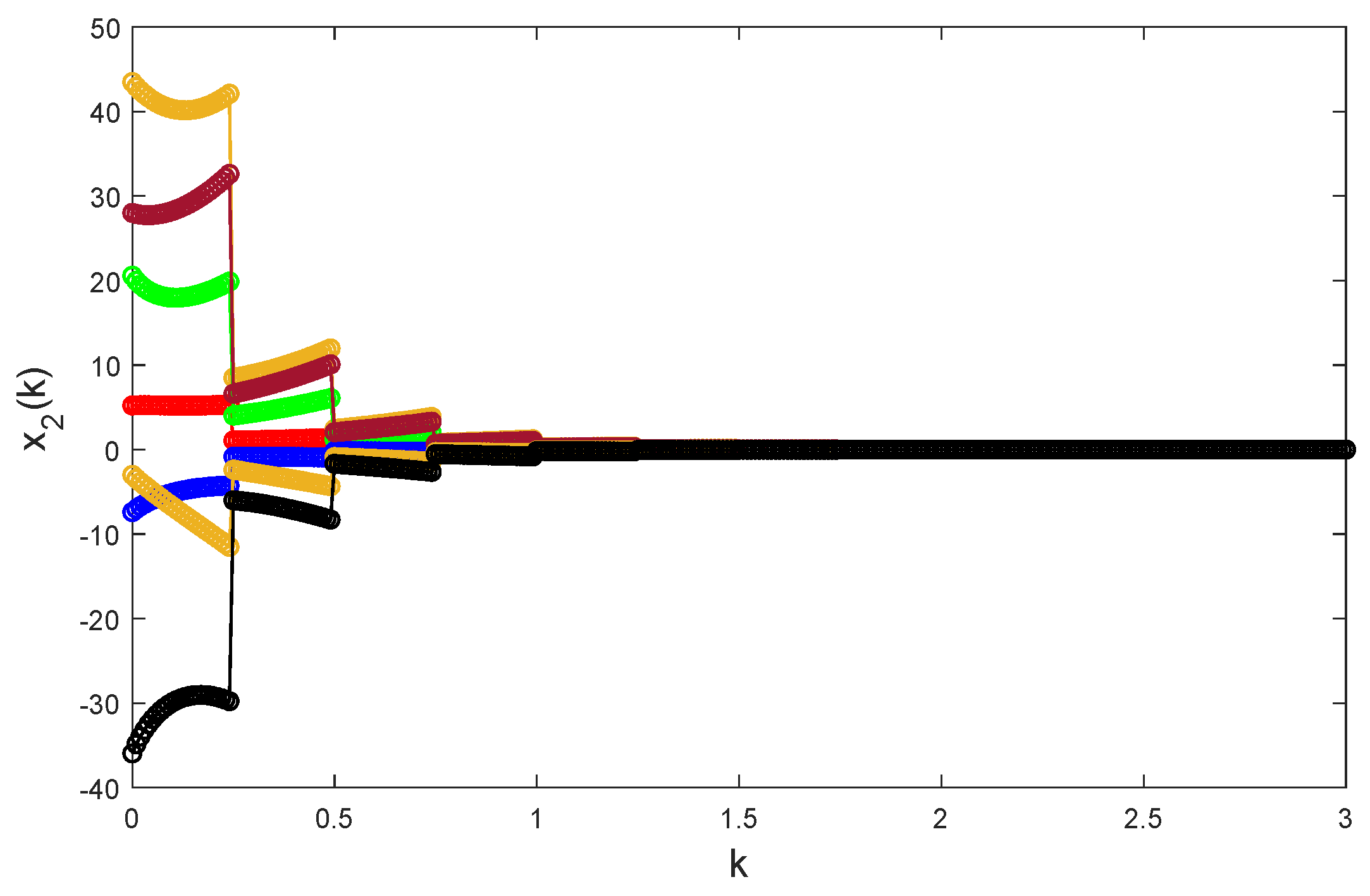
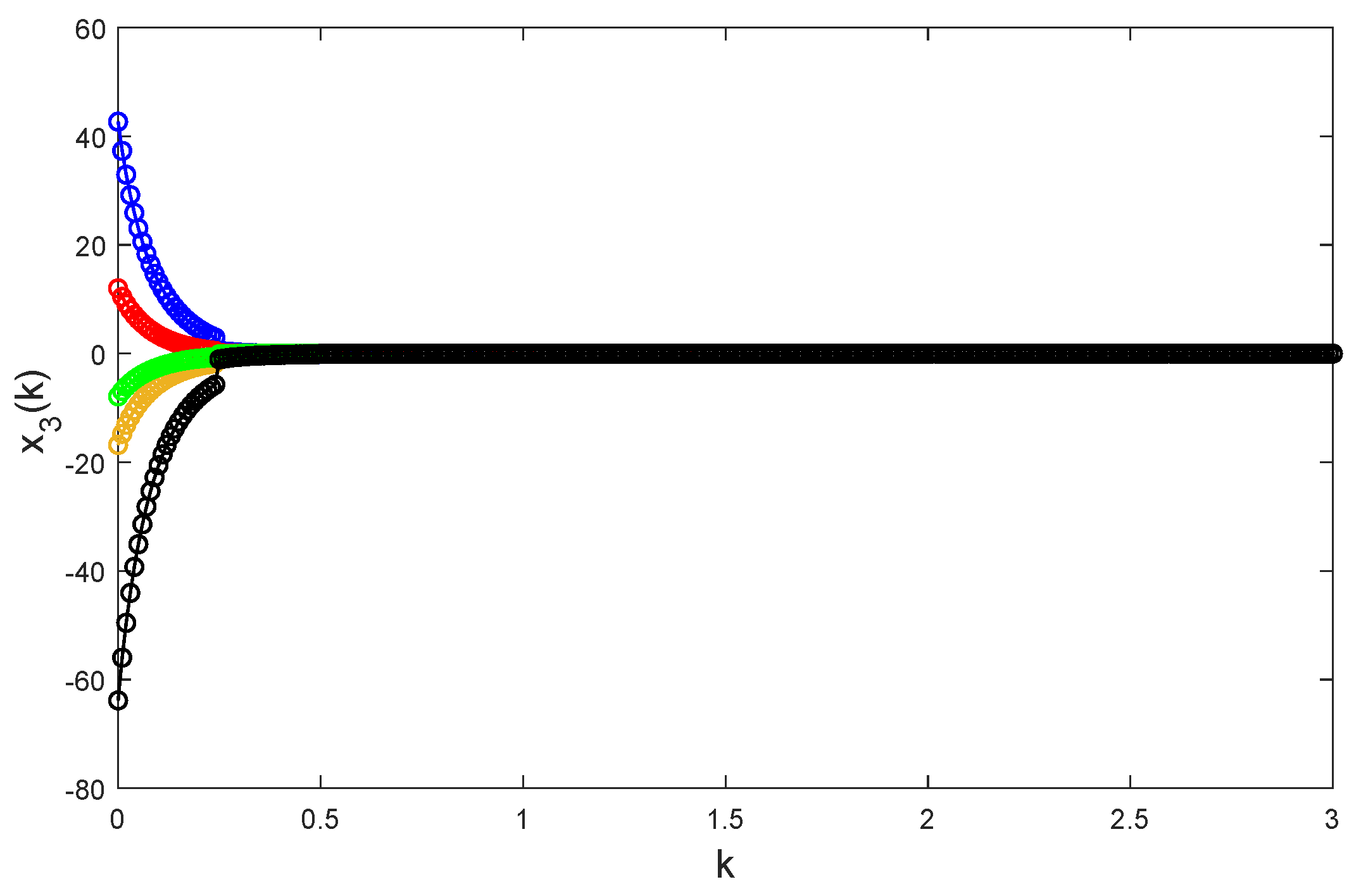
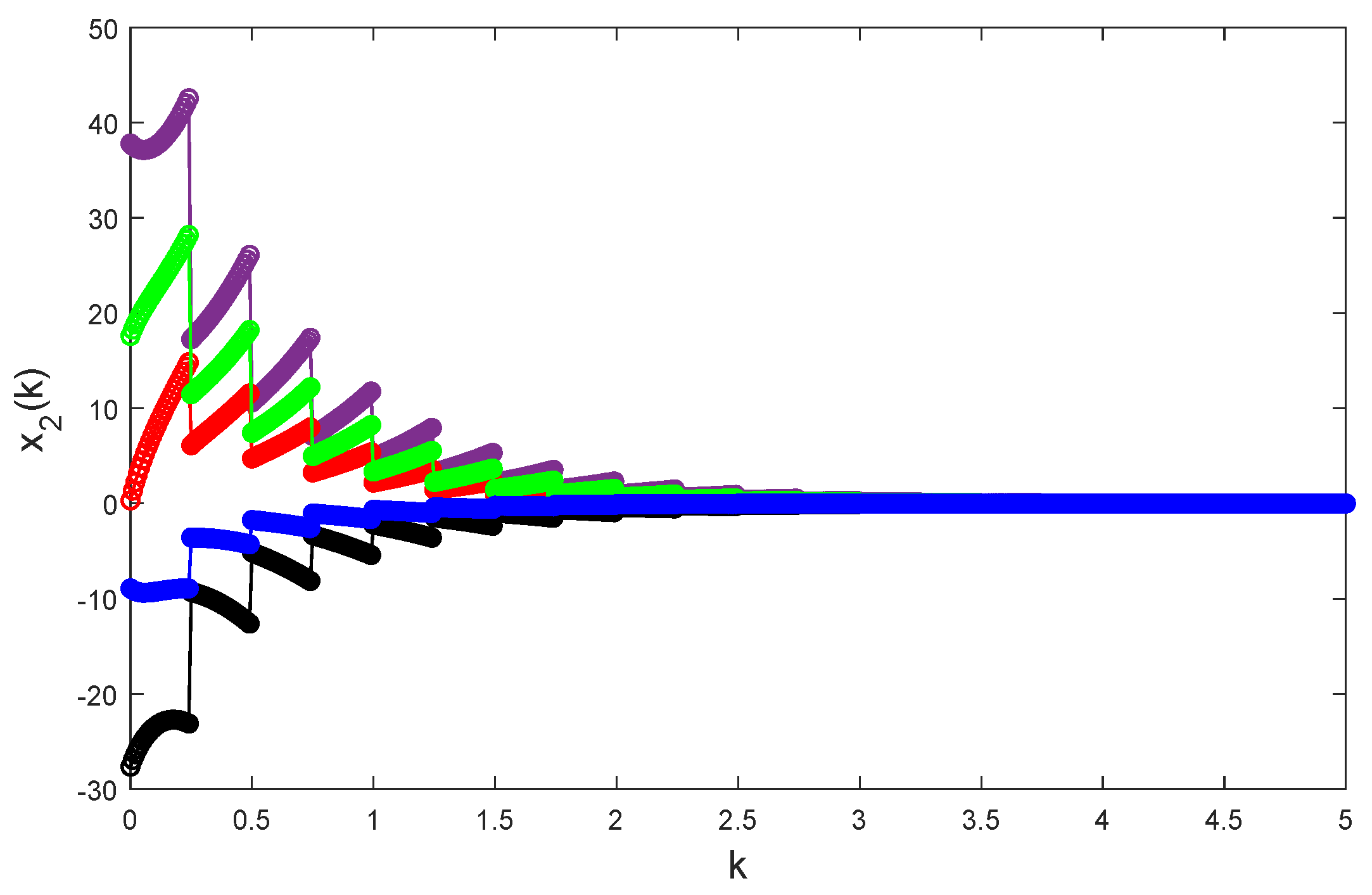
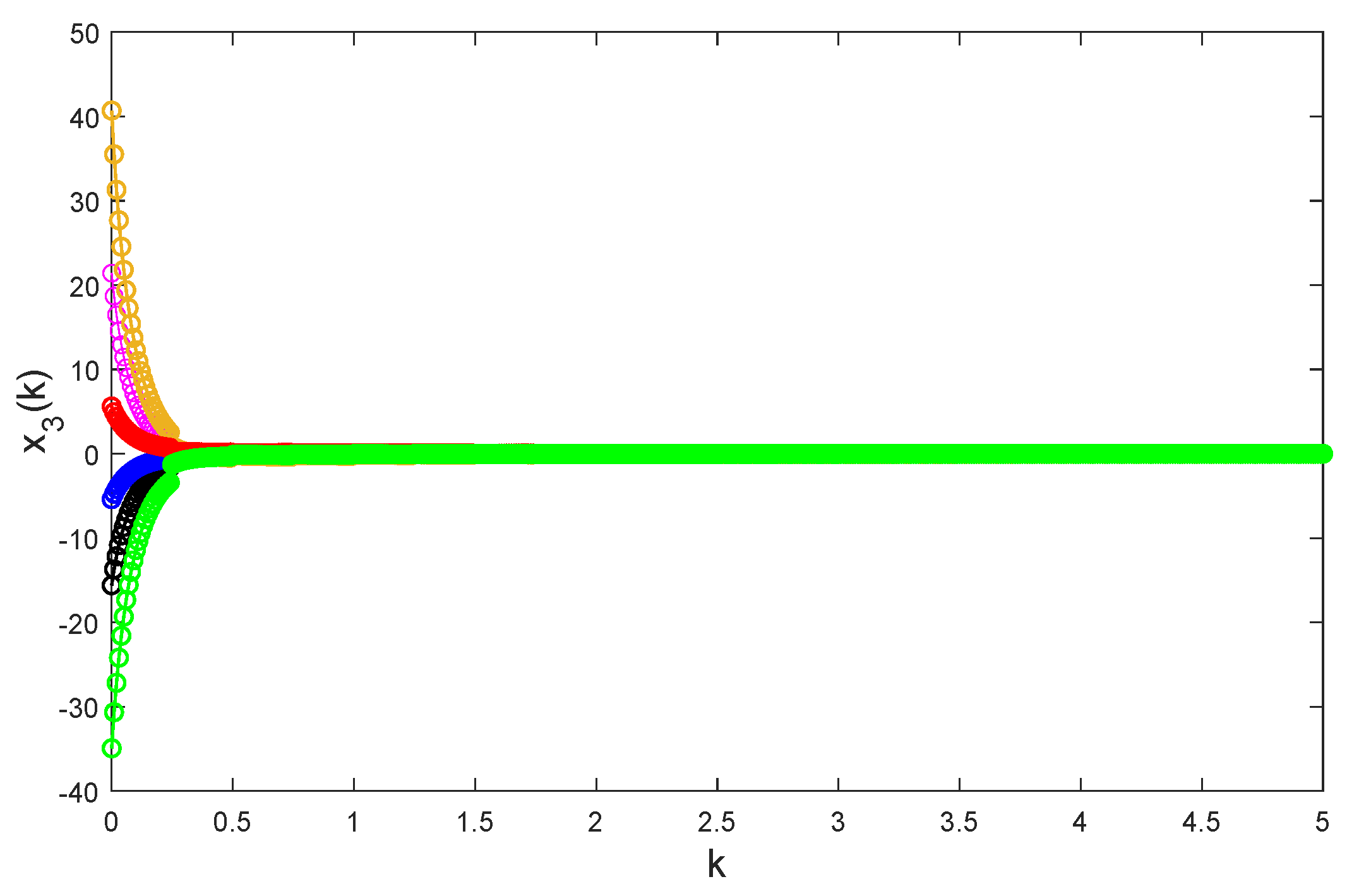
, it is apparent that Chua’s model Equation (
24) is unstable, see
Figure 4,
Figure 5 and
Figure 6.
This example aims to design an instantaneously impulsive controller of global exponential stabilization for model Equation (
24). Adding the impulsive impacts into model Equation (
24), we obtain
where
,
and
are defined as in Equation (
16),
. According to Algorithm 2, an impulsive controller of global exponential stabilization for model Equation (
25) is designed as below
It computes , , , .
Choose and compute .
Calculate and .
By (H2), compute .
Select
,
.
fulfills (H2). By Theorem 1, Equation (
16) will be globally exponentially stable under the designed controlling law below
That is, Chua’s model Equation (
25) is an impulsive controlled stabilization system of Chua’s model Equation (
24).
| Algorithm 2 Instantaneously impulsive controller |
Step 1: Compute the values , , , . Step 2: Choose that a suitable set fills and compute . Step 3: By the results in Steps 1–2, calculate and . Step 4: Based on the calculated values in Steps 1–3, compute by employing relation . Step 5: Select causing for a small preset constant , e.g., , etc. In consequence, fulfills (H2). By the above process and Theorem 1, Equation ( 16) will be globally -exponentially stable under the above-designed controlling law .
|
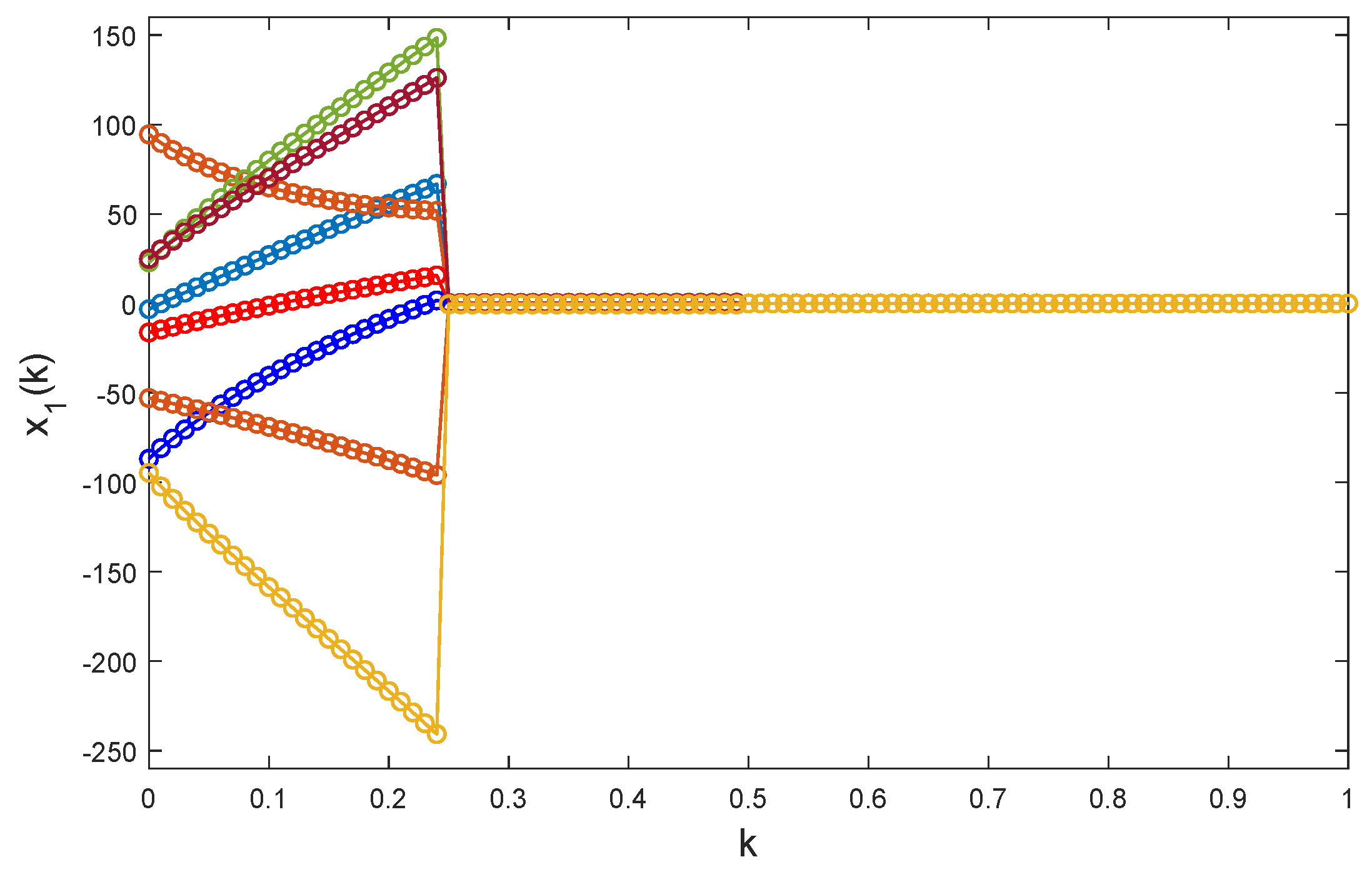
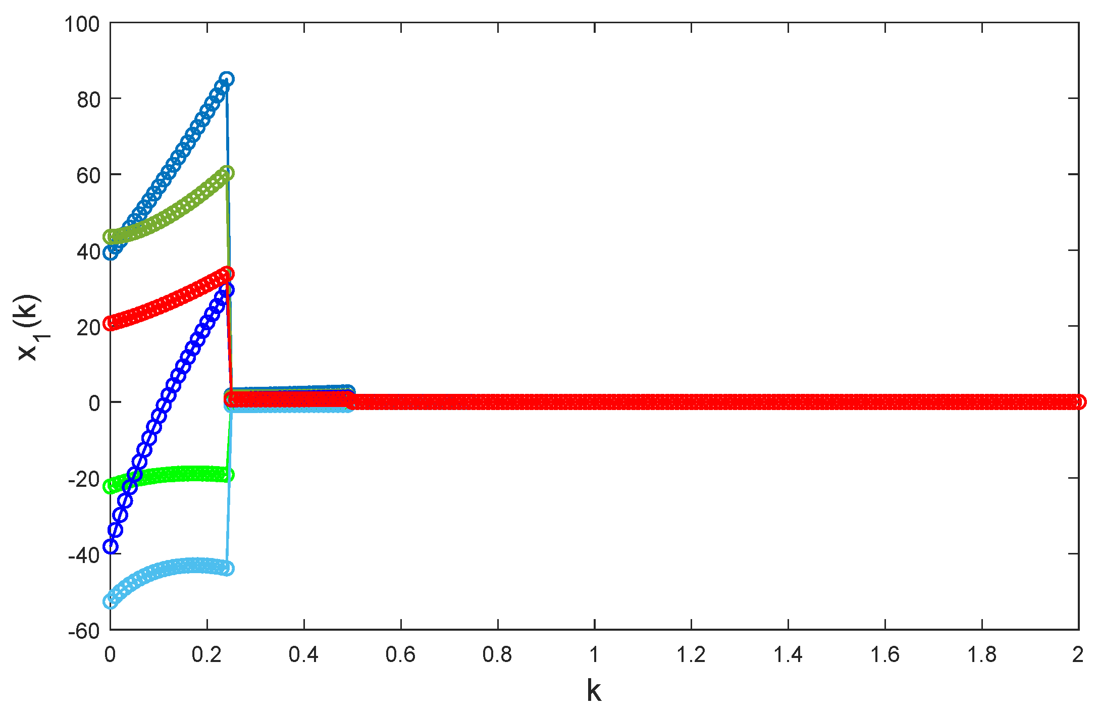
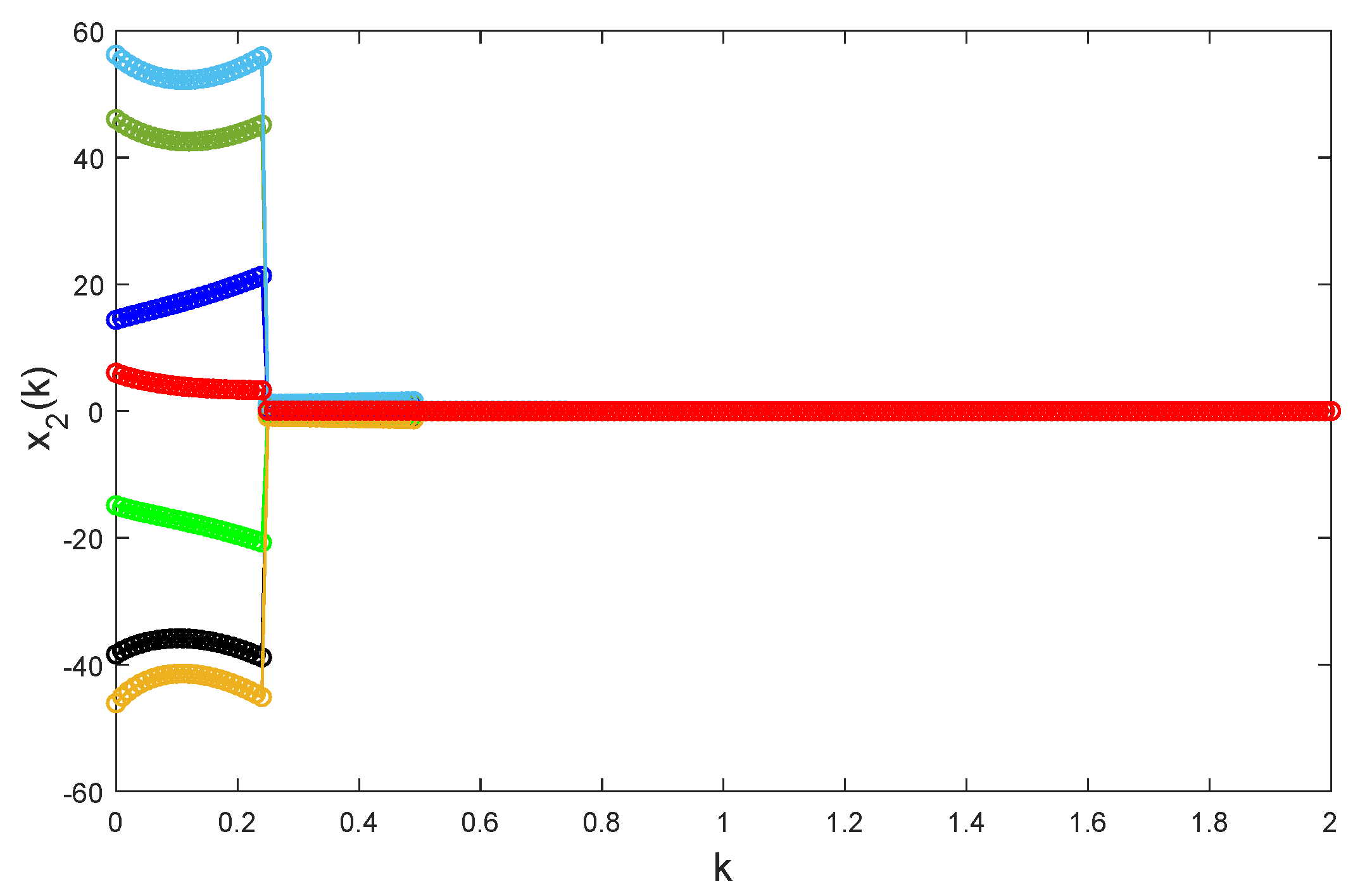
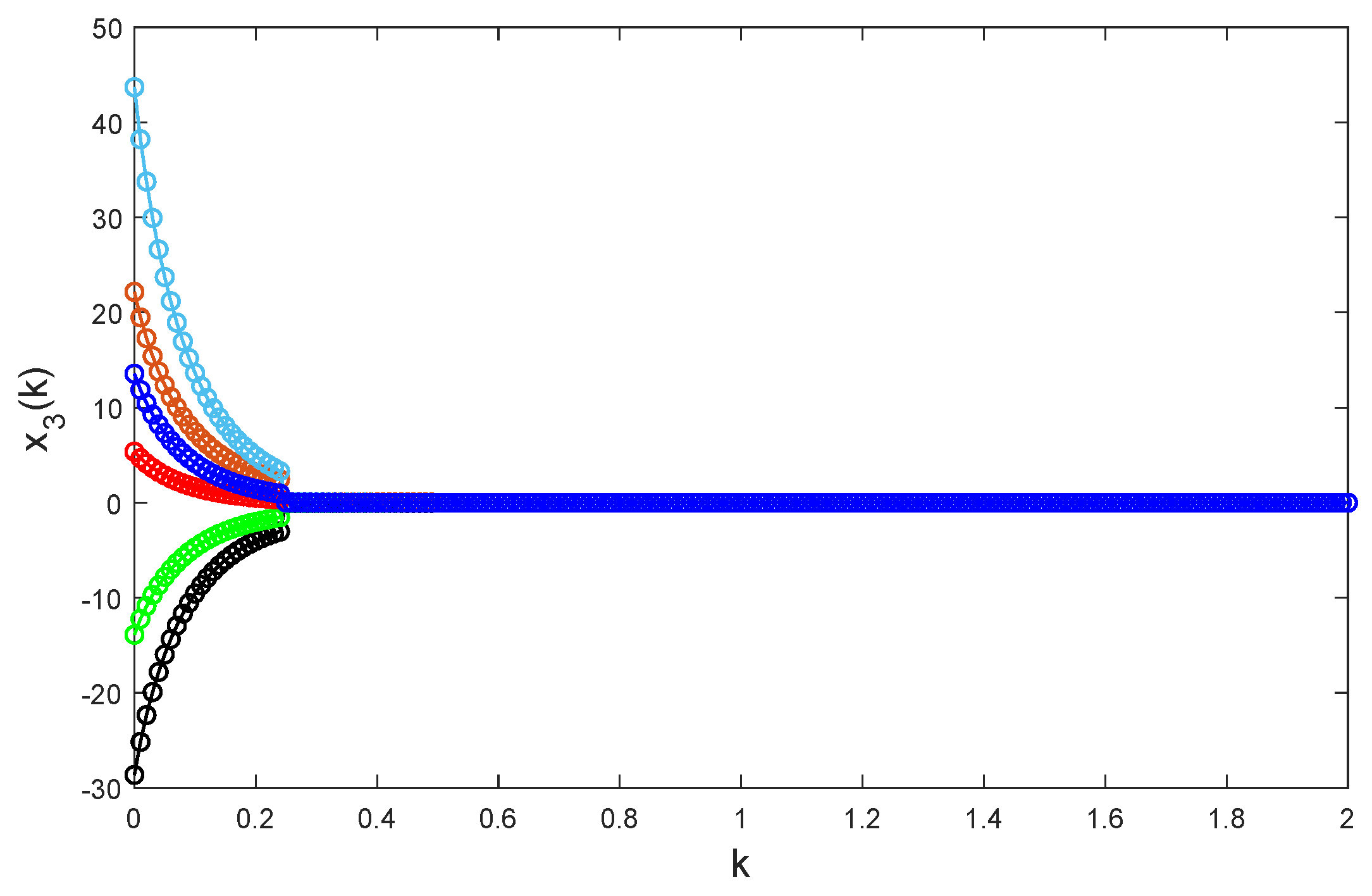
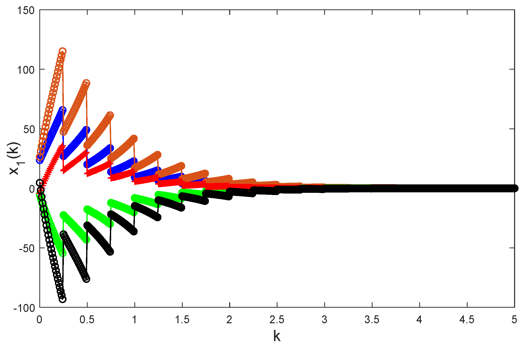
Taking random initial values and
,
Figure 7,
Figure 8 and
Figure 9 depict the trajectories of solutions to model Equation (
25) under controlling law Equation (
26). The images show that model Equation (
25) under the impulsive controlling law Equation (
26) is globally exponentially stable.
Remark 10. With the help of Equation (13), refs. [19,20] were devoted to discussing a variety of dynamic behaviors for Equation (17) without impulses, e.g., periodicity, almost periodicity, stability, randomness, etc. Almost no research involved an investigation of pulse controllers. The work of this paper gets rid of the rigid limitation for . This point exceeds previous works [19,20] and it is more beneficial and convenient for practical applications in science and engineering. Remark 11. By adding impulsive impacts to Chua’s model Equation (24), model Equation (25) under controlling law Equation (26) becomes globally exponentially stable. Thus, impulsive control is an effective method, which makes unstable systems stable. Remark 12. Assumption (H2) is a sufficient condition ensuring the global exponential stability of Equation (16). In other words, there exist controlling laws not satisfying (H2), which are able to ensure the global exponential stability of (H2), please see Figure 10, Figure 11, Figure 12, Figure 13, Figure 14, Figure 15, Figure 16, Figure 17 and Figure 18. 5. Conclusions and Perspectives
On the basis of Mittag–Leffler Euler differences of nonlocal differential systems, the piecewise discrete-time nonlocal operator is newly introduced and a nonlocal discrete-time system with short memory is formulated. From the viewpoint of control theory, this article is devoted to designing an instantaneously impulsive controller to stabilize exponentially the piecewise nonlocal discrete-time system. As an example of applications, the theory and method in this article can be applied in discussions of nonlocal discrete-time Chua’s oscillator and other practical models.
In the research process, the properties of the parameters of Equation (
6) in (K1)–(K9) are crucial. Further, the piecewise feature of continuous-time or discrete-time models is an important character of the studied model. Together with the impulsive discrete variation-of-constants formula in Lemma A1, it is easy to discuss the global dynamics of the nonlocal discrete-time instantaneously impulsive oscillator such as Equation (
16). Finally, the methods in this paper can be applied in the study of other practical models such as the time-fractional advection–reaction–diffusion equation, Burgers’ equation, neutral equations, the switching system, the model of the gemini virus, etc.
A few open theses can be considered further in order:
Expansions of the main results to higher or infinite dimensional systems.
Expansions of the results to other concepts of nonlocal discrete-time systems, e.g., Riemann–Liouville, Grünwald–Letnikov, etc.
Expansions of the results to higher order, e.g., , etc.
Further consideration of the practical factors, e.g., time delays, Markovain jumps or stochastic distributions, etc.
The further optimization of impulsive controlled assumption (H2).

