Modeling Porosity Surface of 3D Selective Laser Melting Metal Materials

Abstract

The most popular method for additively printing metal components is selective laser melting (SLM), which works well for creating working models and prototypes. A fine metal powder, often (stainless) steel or aluminum, serves as the initial material. A very accurate laser is used to melt this layer by layer. The most important factor here is the short throughput time in comparison to milling. Selective laser melting becomes increasingly valuable as geometry becomes more complex. Presented study models the porosity of 3D SLM of metal materials using genetic programming and network theory. We used fractal dimensions to determine the complexity of the microstructure of selective laser melting specimens. The method’s usefulness and efficiency were confirmed by experimental work using an EOS M 290 3D printer and EOS Maraging Steel MS1. This study then presented a novel viewpoint on porosity and has important ramifications for additive manufacturing quality control, which could improve the accuracy and effectiveness of 3D metal printing. The goal was to present a modeling porosity of 3D SLM of metal materials by using a method of intelligent system.

1. Introduction

It is claimed that additive manufacturing (AM) [1], frequently known as 3D printing [2], is a technology that can produce anything by using digital models that are captured by a computer or 3D scanner to create three-dimensional items. While 3D printing employs additive techniques that use chemicals, light, electron beams, or glue to build up layers of material, traditional manufacturing often uses subtractive procedures like cutting, drilling, milling, and grinding. The impact of 3D printing on producers, consumers, and owners of intellectual property rights is immense, and it radically upends established technologies and industrial principles. Although this technology enables manufacturers to quickly prototype complex ideas and builds final parts using drastically diverse techniques, it also makes it possible for anybody to replicate existing product designs and produce, use, and distribute them without the original creator’s consent. Businesses that construct and use 3D printers in this additive manufacturing environment confront new challenges with regard to their copyrights, trade secrets, trade dress, patents, and trademarks. This technology impacts nearly all product design rights holders, and they require direction when making intellectual property judgments. In order to create a three-dimensional object, 3D printing is a process that uses a computer to determine the shape of a thin cross section using three-dimensional (3D) CAD data. The materials are then layered according to the computation’s findings. Due to the availability of inexpensive models for individuals, additive manufacturing technology is gaining popularity and has been dubbed “even individuals can become manufacturers.”

One of the most intricate and remarkable technologies available in rapid prototyping is selective laser melting [3]. Only the CAD data were used to make inserts, models, and intricate patterns that cannot be made with traditional techniques. 3D Activation provides you with steel in SS420 and 1.4404 (L 316) as well as the metals copper, bronze, brass, and aluminum for the SLM 3D printing process. There are several potential alloys, including bronze, nickel, silver, and gold. In the aerospace sector, 3D models constructed of aluminum are especially sought after for prototypes because of their resilience to mechanical and dynamic loads. An alloy consisting of 89.5% aluminum, 10% silicon, and 0.5% magnesium is used at 3D Activation. Conversely, jewelry printing is the primary usage for copper, bronze, and brass. These metals’ exquisite designs are valued by designers and artists, and 3D printing technology makes it feasible to create delicate shapes that are not achievable with traditional manufacturing techniques. Both SS420 and 1.4404 (L 316), special steel alloys, are known for not rusting. SS420 is also notable for its strong heat resistance, while 1.4404 (L 316) stands out for its excellent corrosion resistance and high ductility. Titanium (Ti64) components manufactured by the SLM technique satisfy the ASTM F1472, ASTM B348, and ISO 5832-3 standards [4,5,6] for chemical composition. The 3D material Ti64 is mostly utilized in industrial applications due to the severe physical and chemical requirements imposed on it. Titanium is also becoming more and more popular. Titanium’s exceptional corrosion resistance and low weight are especially valued in aircraft, while its biocompatibility makes it the perfect material for medical technologies. With a precision of 0.5 mm, the Ti64 alloy used in 3D Activation allows wall thicknesses as low as 0.3 mm. Filigree shapes may be created with the same ease as intricate structures and geometries thanks to 3D printing’s selective laser shear melting process, which also makes undercuts and cavities conceivable. Metal 3D printing is opening up new possibilities in metal production. The potential for a tool-free manufacturing process is also made possible by 3D printing with SLM. Metal 3D printing makes it feasible to create very high-quality display models because of the expansive installation spaces that 3D Activation can provide.

Fractal geometry [7], roughly speaking, deals with complex shapes found in nature (such as broccoli in the supermarket). “Fractal” refers to a geometric structure that has a special property called “self-similarity”, and more specifically, to a structure in which the same shape as a whole is reproduced when the whole figure is broken down into several parts. The concept was invented by French mathematician Benoît B. Mandelbrot. One example is a coastline, which has the interesting property of looking the same on maps of any scale. This is apparently called statistical self-similarity. I wonder if it is easy for elementary school students to understand. Well, there are shapes where many parts of the same shape come together to form a larger, identical shape. You can see this when you zoom in on a coastline on a map, or when looking at the way tree branches branch out. Each part can be expressed by a simple mathematical formula, and by repeating them, they can form a whole. You can also see this in the spread of blood vessels and nerves in animals.

Network theory [8] provides a set of techniques for analyzing graphs. The current range of applications of network theory is wide, ranging from the analysis of various problems in engineering fields, such as road networks, railway networks, electrical circuit networks, and communication networks, to network model analysis in social sciences and humanities fields such as sociology, economics, and psychology. In electrical circuit networks, the current and voltage flowing through each element can be associated with the edges of the network, and in transportation networks, the road network, railway network, and the number of vehicles, passengers, and cargo passing through them can be associated with each edge [9]. In fields such as behavioral science and social psychology, various states or members of each group can be represented as network vertices; causal relationships and mutual relationships between them can be represented as edges, and the degree of communication and influence between states or members can be quantified and associated with each edge.

A computer can scan vast volumes of data, identify patterns buried in the data, and develop rules for evaluating unknown data thanks to a technology called machine learning [10]. It has gained popularity as a technology that is positioned as a component of “AI (artificial intelligence)” in recent years. Currently, this technology is starting to affect a number of disciplines, including biology, autonomous driving, image processing, and financial engineering. Machine learning is a system in which a computer is fed huge amounts of data and analyzed based on various algorithms. By repeatedly teaching a computer, it is possible to find hidden features and patterns in the data. The algorithms used here vary depending on the characteristics and purpose of the data being fed into the computer, and it is necessary to prepare algorithms that are appropriate for each purpose.

Authors in [11] researched on a new approach based on the use of a Regression Convolutional Neural Network (RCNN) algorithm to predict the percentage of porosity in CT scans of finished SLM parts, without the need for subjective difficult thresholding determination to convert a single slice to a binary image. The problem of evaluating porosity in SLM components is difficult, and the disadvantage of the current gray value analysis approach is the subjectivity and difficulty of choosing a consistent grayscale threshold for binary image conversion in order to detect porosity. Addressing this issue, the study in [12] explored the efficacy of in situ thermography, particularly short-wave infrared thermography, for detecting and predicting porosity during manufacturing. Paper [13] used a Short-Wave Infrared (SWIR) camera to record the temperature history for parts manufactured with Laser Powder Bed Fusion processes by process of AM. The porosity from a cylindrical specimen is measured by ex situ micro-computed tomography (μCT). In study [14], its authors investigated the methods for controlling porosity in thermal pipes manufactured using SLM technology. In [15], its authors used Finite element modeling (FEM), microscopy, X-ray computed tomography (CT), and mechanical property tests to study the microstructure, porosity, and mechanical properties of an AlSi10Mg alloy produced by SLM.

The aim of this study is to present a modeling porosity of 3D SLM of metal materials by using method of intelligent system.

2. Material Preparation and Experimental Work, Methodology, and Modeling

We used the EOS M 290 SLM machine (Figure 1) [16]. The EOS M 290 Basic Training app allows users to engage with a full-size model of the EOS M 290 and familiarize themselves with its key components through an immersive augmented reality experience. EOS claims that its first Extended Reality (xR) program for the EOS M 290 system, Additive Minds Academy, helps users accelerate their learning curves. It is claimed that the EOS M 290 Basic Training app will save money for businesses by allowing both new and current staff to learn systems more quickly, from any location, and even prior to delivery.

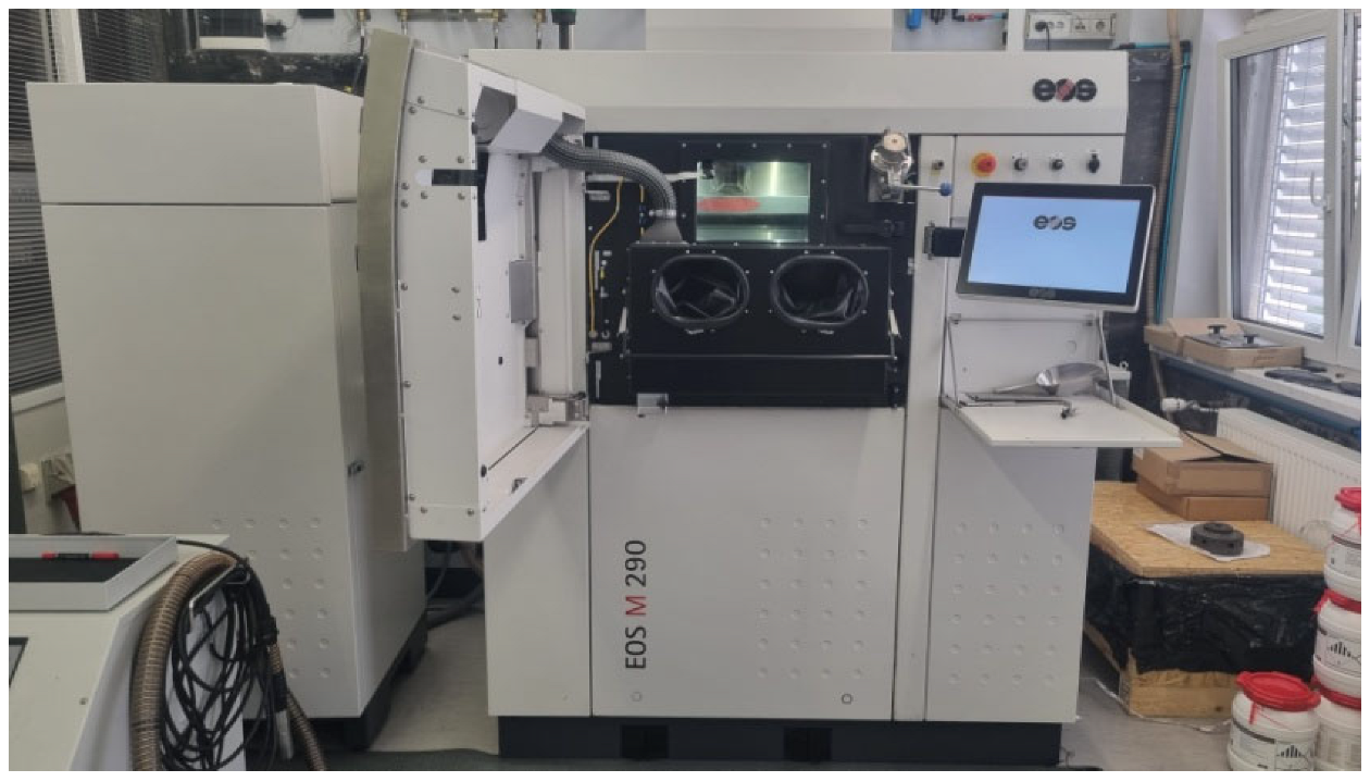
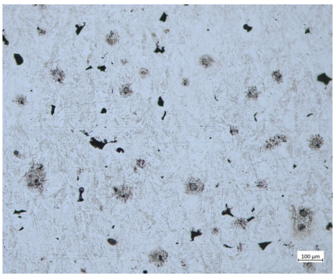
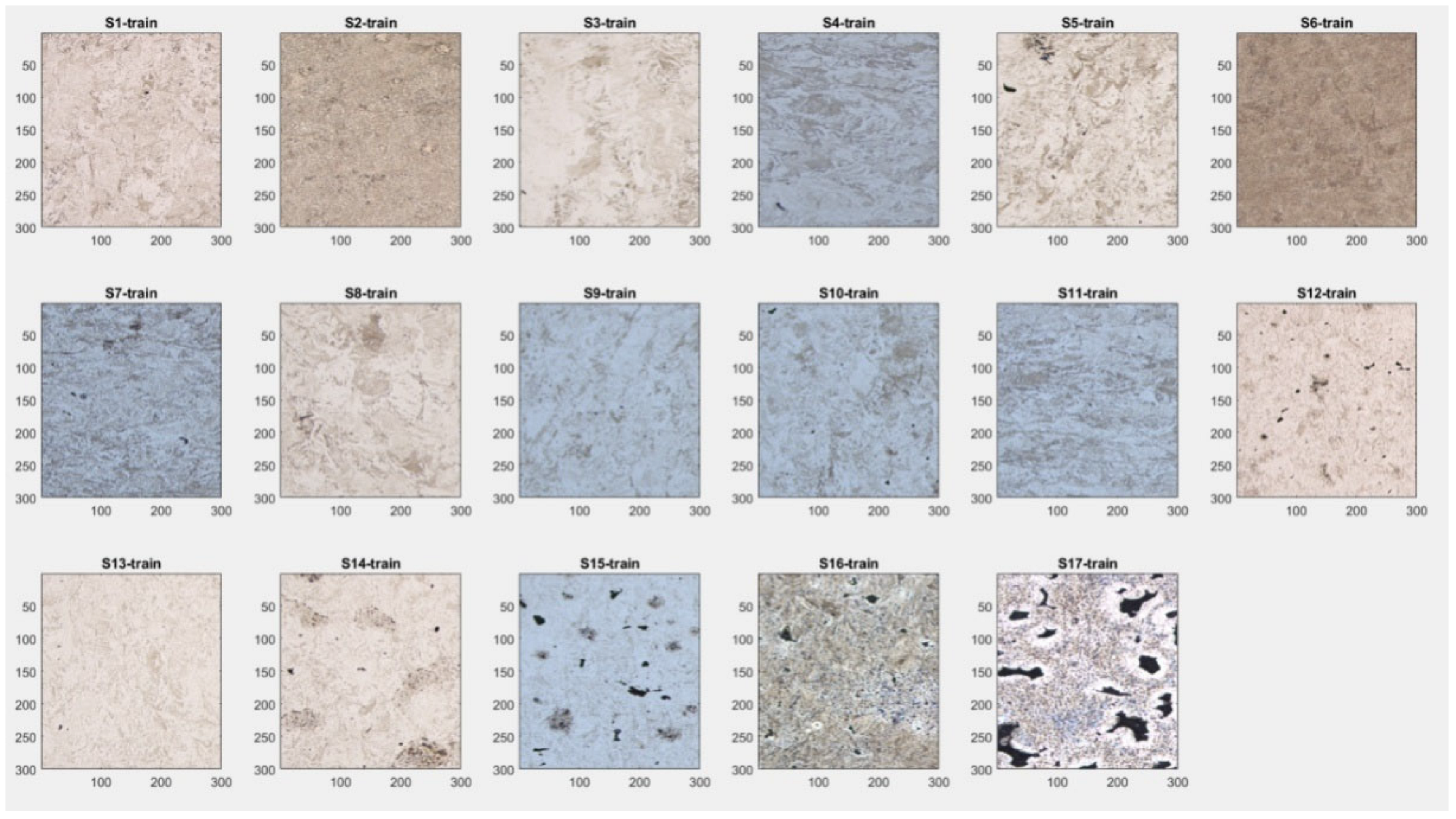
2.1. Experimental Work and Material Preparation

We used material EOS Maraging Steel MS1 [17]. Ultra-high-strength maraging steel of tooling grade is EOS Maraging Steel MS1. Through the formation of intermetallic phases and precipitates after heat treatment, its exceptional qualities are made possible. Its alloying of titanium, nickel, cobalt, and molybdenum produces a great material for additive manufacturing with balanced qualities and minimal distortion. These characteristics allow for its successful usage in a variety of applications, such as cold and hot working and injection molding. Figure 2 present microstructure of SLM specimen.

2.2. Methodology

The SLM specimen’s microstructure is extremely intricate. We cannot use classical Euclidian geometry [18], but we must use fractal geometry in characterizing the complexity of microstructure of a SLM specimen.

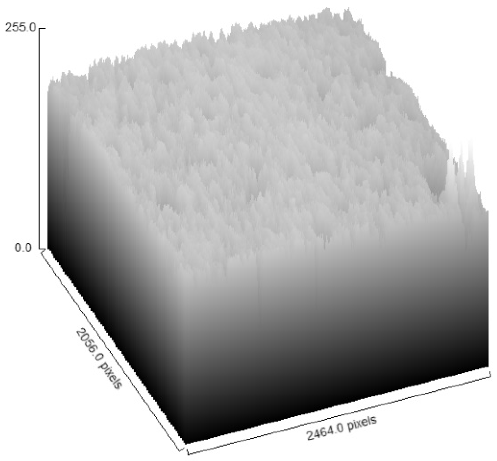
2.2.1. Fractals

In fractal geometry, self-similarity or self-affinity and fractal dimensions are important [19]. We used the slit island method using area–perimeter relationships for calculating fractal dimension. In Figure 3, the white object represents a lake, and the shaded object represents an island. Island area, A, is computed by counting the number of black pixels. Perimeter, P, is estimated by counting the number of pixels covering the perimeter. The area perimeter relationship is given as follows [20]:

$$\mathrm{P}={\mathrm{P}}_0\times {\mathrm{A}}^{\mathrm{D}2}$$

(1)

$$\log (\mathrm{P})=({\mathrm{P}}_0)+{\displaystyle \frac{D}{2}}\times \log (\mathrm{A})$$

(2)

where D is the fractal dimension of the island’s shoreline and P₀ is the scaling constant.

Figure 3 present connections between area and perimeter. Pixel ‘islands’ landscape. Each island’s area is shaded, and a solid black line denotes its circumference.

Limitations of the method:

• The digital image’s pixel is rectangular, which causes ‘rectangularization’ for tiny islands (A < 30) to produce erroneous estimations of D.
• There are also issues with edge effects, with biased estimations of D provided by islands that touch the image’s edges.
• “Staircase” impact of the 45° orientation’s perimeter since more pixels are needed.

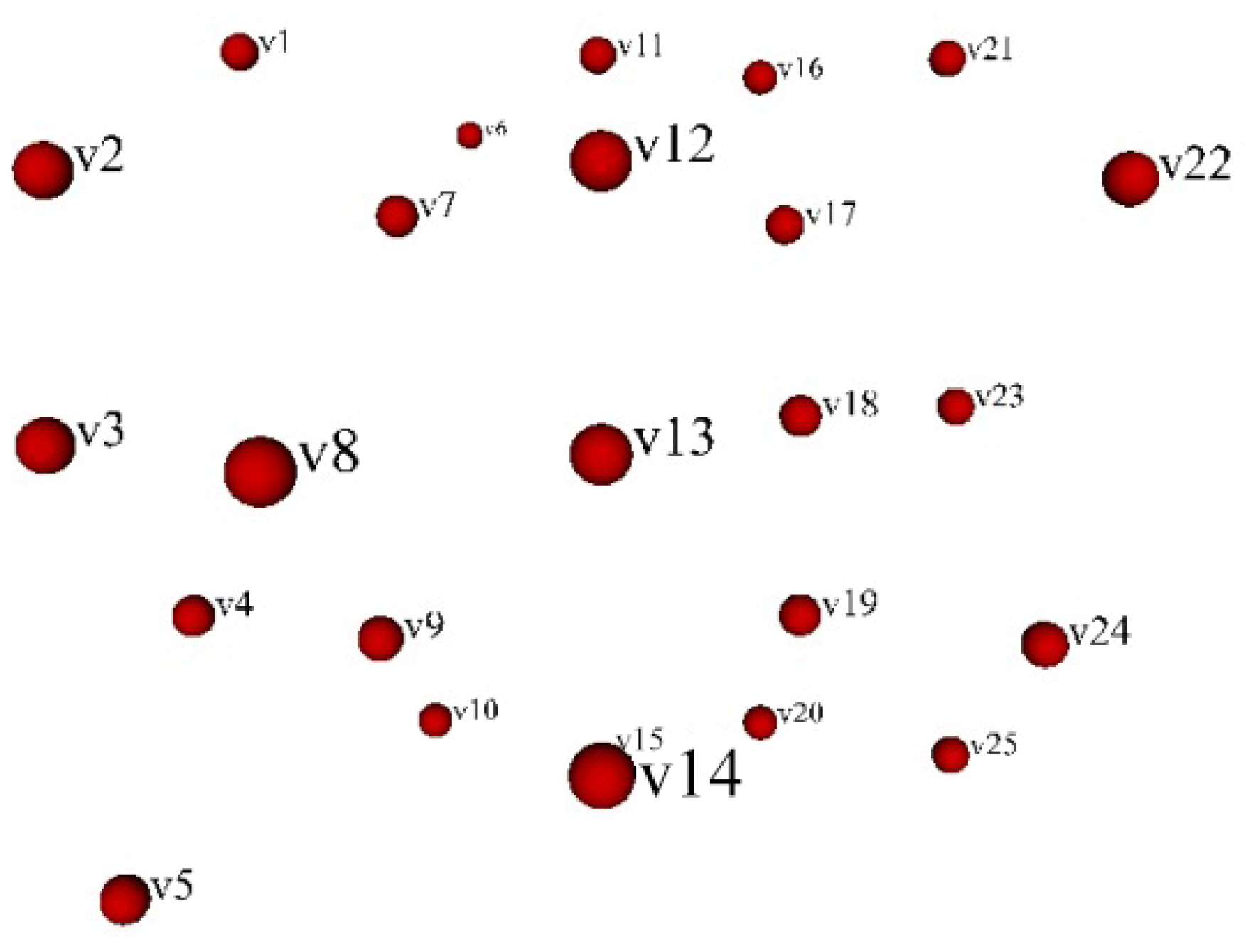
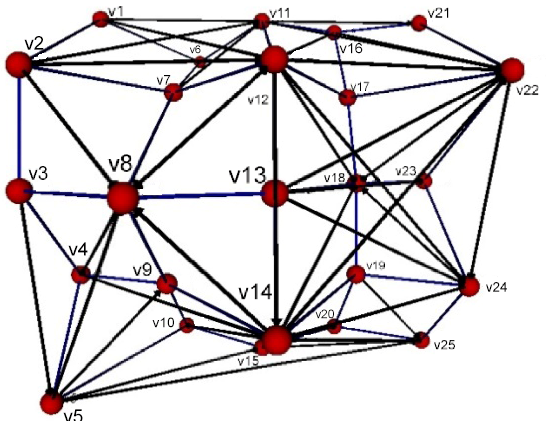
2.2.2. Network Theory

A new technique for identifying patterns through the use of network theory or graph theory was created [21]. This graph comprised a pair of a set of points V and a set of edges E connecting the two points. It is expressed as G = (V,E). Points are called vertices or nodes, and edges are called arcs or edges. A graph is a model that represents a combinatorial structure. Figure 4 to below presents a 3D graph of the microstructure of a SLM specimen previously shown. Visibility: If the open-line segment connecting two points, p and q, does not cross the interior of any obstruction, we can say that the points are mutually visible. A visibility graph is a graph of indivisible locations, typically for a set of points and barriers in the Euclidean plane. In the graph, every node denotes a point location, and every edge shows a discernible link between them. In other words, an edge is drawn on the graph between two sites if the line segment that connects them does not encounter any obstructions.

Figure 5 presents the vertices of the graph in Figure 4 for network 5 × 5 (for better visualization).

Babič et al. [22] presented a solution for constructing a visibility network in a 3D space. Figure 6 presents the results of the problem of constructing a visibility network in a 3D space. We used the statistical topological property of the density of the visibility network from SEM images. The percentage of possible connections in a network that are really connections is referred to as network density. The density q for each visibility network was calculated by Equation (1):

$$\mathrm{q}={\displaystyle \frac{2m}{n\times (n-1)}}$$

(3)

where m is the number of edges and n is the number of vertices in the visibility network.

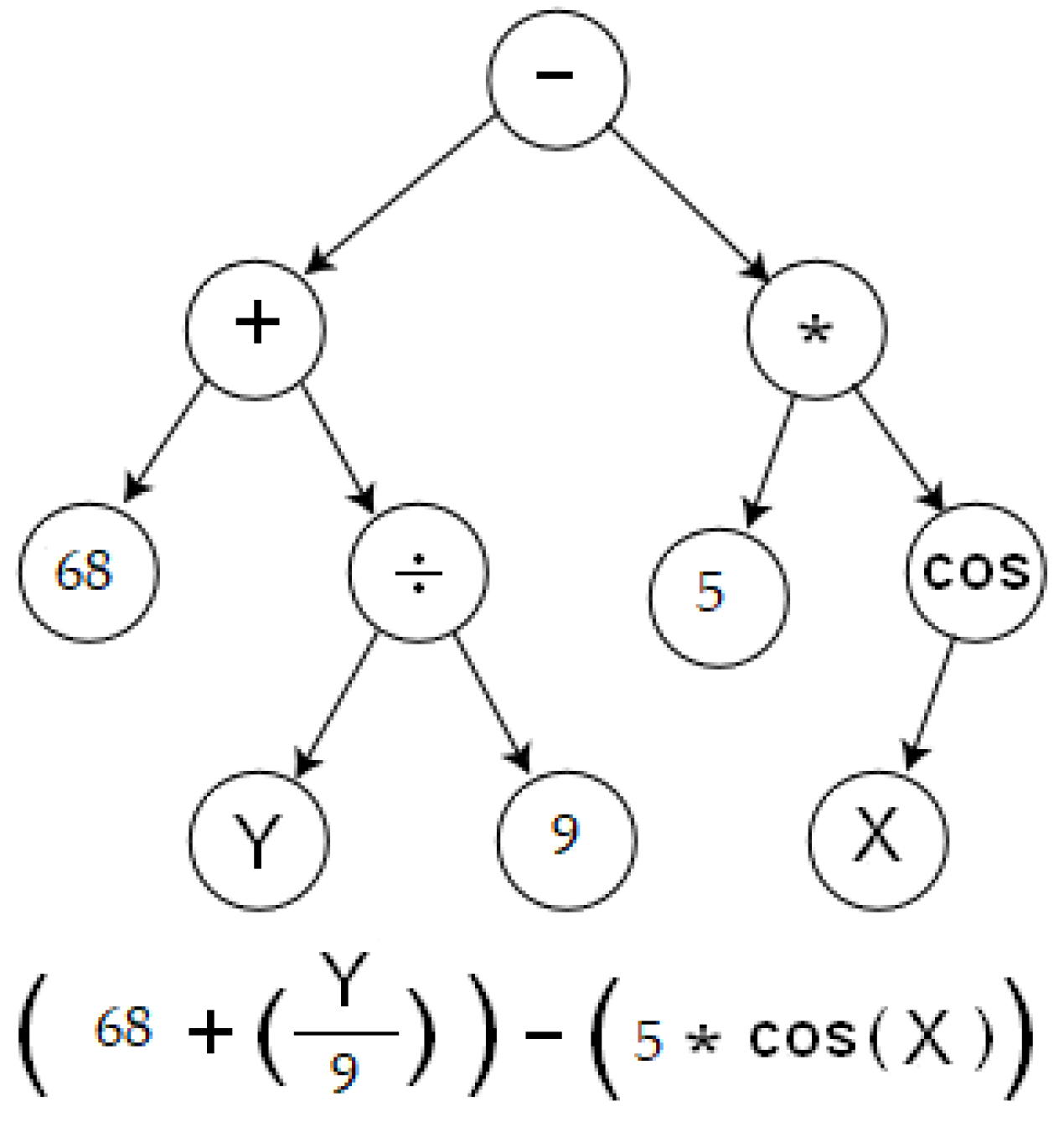
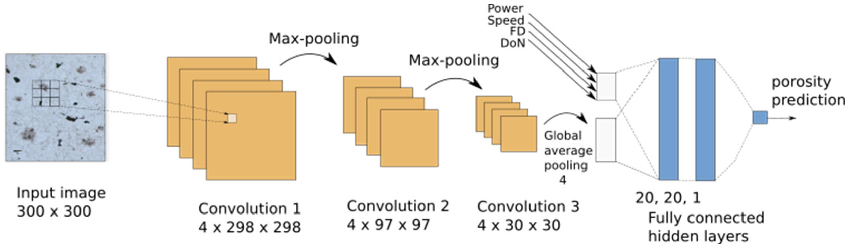
2.2.3. Modeling

For modeling porosity surface of a 3D SLM specimen, we used intelligent system methods, namely genetic programming [23,24,25] and a convolution neural network [26].

The technique of genetic programming (GP) belongs to the group of evolutionary algorithms. These attempt to formalize the natural evolution of living beings into general algorithms. Processes known from biology are projected onto an algorithmic problem. In the special case of genetic programming, the created individuals are viewed as independent programs that are intended to solve a given problem as best as possible according to certain criteria. The implementation of genetic programming can be divided into several, sometimes optional, steps: Initialization, evaluation, selection, recombination, and mutation.

The following Figure 7 is an example of a simple tree program:

A unique kind of artificial neural network, known as convolution neural networks (CNNs), are built on local feature detectors or filters that share their adjustable weights or parameters [27]. CNNs are particularly applicable to signal processing and, most notably, to image processing. In image processing, two-dimensional discrete convolution is applied to all image pixels; this has the effect of digital filtering. Several filters or kernels are usually used in order to detect different low-level features in the input image. Typically, a pooling layer comes after a convolution layer. It compresses information by maximizing or averaging rectangular pixel areas, which efficiently reduces vast volumes of visual data. Both layers, convolution and pooling, can be reapplied several times to further reduce the data. These layers are normally followed by a feed-forward fully connected neural network–multilayer perceptron, the most common type of neural network. It consists of several fully connected layers of processing elements (neurons). These most frequently use sigmoid or relu activations functions. Target variables, which in this case is porosity, are predicted by the output of the last (output) layer.

The specimen photos were trimmed to a consistent 600 × 300 resolution. The left half of size 300 × 300 was used for training (Figure 8) and the right half of size 300 × 300 was used for testing. The images were converted to grayscale. The values were scaled from the [0, 255] interval to the [0, 1] interval.

3. Results and Discussion

Table 1. Parameters of SLM specimens.

Specimen	Power (W) X1	Speed (mm/s) X2	FD X3	Density η X4
S1	320	1000	1.52	0.25
S2	320	1150	1.47	0.54
S3	320	1300	1.69	0.73
S4	270	850	1.75	0.62
S5	270	1000	1.71	0.72
S6	270	1150	1.54	0.65
S7	270	1300	1.51	0.56
S8	220	700	1.68	0.81
S9	220	850	1.82	0.92
S10	220	1000	1.65	0.62
S11	220	1150	1.71	0.38
S12	220	1300	1.84	0.67
S13	170	700	1.59	0.36
S14	170	850	1.45	0.56
S15	170	1000	1.54	0.38
S16	170	1150	1.63	0.87
S17	170	1300	1.57	0.75

displays the properties of the SLM specimen. The first column lists specimens with S1 through S17. The laser’s power is displayed in W in the second column; this parameter is indicated by X1. The second column displays the laser’s speed in mm/s; this parameter is represented by X2. The third column displays the complexity of the SLM specimen; this feature is denoted by X3. The fourth column shows the density of visibility network of the microstructure of the SLM specimen; this parameter is denoted by X4. The hatch distance used was 0.11 mm.

Table 2. Porosity of SLM specimens.

Specimen	Porosity (%)
S1	0.02
S2	0.04
S3	0.17
S4	0.04
S5	0.07
S6	0.06
S7	0.52
S8	0.07
S9	0.03
S10	0.08
S11	0.34
S12	1.79
S13	0.35
S14	0.07
S15	1.37
S16	4.06
S17	7.33

shows the porosity of the SLM specimen; Y is expressed in %. The forecast porosity of the SLM specimen with GP and CNN are shown in

Table 3. Prediction porosity of SLM specimens with GP and CNN.

Specimen	GP Porosity	CNN Porosity
S1	0.019932	0.0529
S2	0.040051	0.0163
S3	0.174835	0.1362
S4	0.042027	0.0739
S5	0.044027	0.0603
S6	0.057547	0.1635
S7	0.259549	0.4482
S8	0.074928	0.0511
S9	0.029815	0.2078
S10	0.07989	0.2698
S11	0.350045	1.1405
S12	0.061404	2.8863
S13	0.049603	0.4912
S14	0.072834	0.2193
S15	0.042733	1.1446
S16	4.33582	2.8921
S17	0.073286	6.1677

. The genetic programming model for porosity is represented by the second column, while the convolution neural network model for porosity is shown in the last column. Specimen S1 has minimum porosity, 0.02%. Specimen S17 has maximum porosity, 7.33%. Equation (4) presents the model of genetic programming.

GP model for porosity of SLM specimens:

$$\begin{gathered} {\displaystyle \frac{1}{\mathrm{X}1}}0.297929\left(35.042-{\displaystyle \frac{16.2854\left(1-\mathrm{X}3+\mathrm{X}4\right)}{\mathrm{X}4\left(-\frac{8.14268}{\mathrm{X}4}+8.44651\times 4\right)}}+{\displaystyle \frac{\left(\mathrm{X}3-\mathrm{X}4\right)}{\mathrm{X}3-8.44651\times 4-\frac{8.44651\times 4}{-2\times 3-\mathrm{X}4}}}-{\displaystyle \frac{27.331}{\left(1+\mathrm{X}4\right)\left(\mathrm{X}4+\frac{\left(-\frac{8.14268}{\mathrm{X}4}+8.44651\times 4\right)}{\mathrm{X}3}\right)}}+ \\ {\displaystyle \frac{8.44651\times 4}{-2\times 3-\frac{\left(\mathrm{X}4+\frac{\left(-\frac{8.14268}{\mathrm{X}4}+8.44651\times 4\right)}{\mathrm{X}3-\mathrm{X}4}\right)}{\mathrm{X}3}}}-{\displaystyle \frac{1}{-4.1487+\mathrm{X}3}}\left(8.44651\times 4+{\displaystyle \frac{8.44651\times 4}{-\frac{8.14268}{\mathrm{X}3}-\mathrm{X}3+8.44651\times 4}}+ \\ {\displaystyle \frac{\left(9.44651\times 4+\frac{79.79\times 4}{-8.44651-\mathrm{X}3-\mathrm{X}4-\frac{\left(\mathrm{X}4+\left(-\frac{8.14268}{\mathrm{X}4}+8.44651\times 4\right)\right)}{\mathrm{X}3}}\right)}{\mathrm{X}4}}\right)\right) \end{gathered}$$

(4)

Experimental and predicted porosity data are shown in Figure 9.

We have used a convolution neural network to predict porosity on the basis of surface images. Aside from images, some non-image input parameters were applied, such as Power (W), Speed (mm/s), FD, and Density of network η, as shown in Figure 10.

To reduce the image size, a two-dimensional max-pooling (3 × 3) was used after a two-dimensional convolution layer with four kernels and a filter size of 3 × 3. The 2D convolution layer and max-pooling combination was used again to accomplish even more compression. The third convolution layer and an average pooling layer came next, whose output was compressed so that it could be combined with the non-image data. The CNN had 957 trainable parameters or weights, as shown in

Table 4. Structure of the CNN.

Layer (Type)	Output Shape	Param #	Connected to
input_1 (InputLayer)	(300, 300, 1)	0
rescaling (Rescaling)	(300, 300, 1)	0	input_1
conv2d (Conv2D)	(298, 298, 4)	40	rescaling
max_pooling2d (MaxPooling2D)	(99, 99, 4)	0	conv2d
conv2d_1 (Conv2D)	(97, 97, 4)	148	max_pooling2d
max_pooling2d_1 (MaxPooling2D)	(32, 32, 4)	0	conv2d_1
conv2d_2 (Conv2D)	(30, 30, 4)	148	max_pooling2d_1
global_average_pooling2d (Global)	(4)	0	conv2d_2
flatten (Flatten)	(4)	0	global_average_pooling2d
input_2 (InputLayer)	(4)	0
concatenate (Concatenate)	(8)	0	flatten, input_2
dense (Dense)	(20)	180	concatenate
dense_1 (Dense)	(20)	420	dense
dense_2 (Dense)	(1)	21	dense_1

.

Since the target values of porosity were unevenly distributed (most values were below 0.5, while a few of them were larger, with some even above 7). For training and testing, they were logarithmically transformed and scaled to [0, 1]. Due to the small number of samples, the training procedure was performed as an 8-fold cross validation, where 2 samples (17/8) were taken aside 7 times and 3 samples were taken aside once to yield the testing set, while the remaining 15 (or once 14) samples were used as the training set. The testing MSE was a little above 0.01, which implies RMSE is about 0.1, which is quite good. The values were then transformed back.

4. Conclusions

In this article, we presented the modeling porosity surface of SLM specimens. We used genetic programming and convolutional neural network to predict the porosity of SLM specimens. We used fractal geometry to characterize the complexity of the microstructure of a SLM specimen.

One of the most adaptable 3D printing methods is SLM, which may be used to replace materials that are cast, machined, or welded. Nonetheless, 3D metal printing, in particular, offers a number of advantages and is becoming more and more popular in the industry, particularly in terms of building freedom. Because the component is built layer by layer in the desired shape, even difficult-to-process materials can be used. Even very intricate patterns and moving parts can be made using this AM process. Additionally, tool-free production is very fast and reliable. Economic efficiency can be further increased by using as little waste as possible, particularly in metal printing. Nowadays, components may be printed with an accuracy of 0.1 mm thanks to industrial 3D printing. The components of this generative manufacturing technique meet even the most demanding specifications. There is a lot of room for innovation with laser melting. Because design possibilities are no longer limited by production, the time between product creation and commercial launch opens up completely new possibilities. Components that would have been prohibitively expensive or perhaps impossible to manufacture using conventional production methods can now be made, and this is very cost-effective even at small quantities. 3D metal printing is beneficial to not only traditional buyers of high-tech components, like the automotive or aerospace industries, but also for areas such as the mechanical engineering, tool manufacturing, and medical science.

We have predicted porosity from surface photos using a convolution neural network. In addition to pictures, non-image input characteristics including Power (W), Speed (mm/s), FD, and Density of network η were used. There were 957 trainable weights or parameters in the CNN. We determined the microstructure complexity of selective laser melting specimens using fractal dimension. Experiments with an EOS M 290 3D printer and EOS Maraging Steel MS1 validate the method’s effectiveness and use. The study thus offers a fresh perspective on porosity and has significant implications for quality control in additive manufacturing, which may enhance the precision and efficiency of 3D metal printing. This aims to model the porosity of 3D SLM of metal materials using an intelligent system approach.

References

- Groth, J.-H.; Magnini, M.; Tuck, C.; Clare, A. Stochastic design for additive manufacture of true biomimetic populations. Addit. Manuf. 2022, 55, 102739. [Google Scholar] [CrossRef]
- Shahrubudin, N.; Lee, T.C.; Ramlan, R. An overview on 3D printing technology: Technological, materials, and applications. Procedia Manuf. 2019, 35, 1286–1296. [Google Scholar] [CrossRef]
- Soni, N.; Renna, G.; Leo, P. Advancements in Metal Processing Additive Technologies: Selective Laser Melting (SLM). Metals 2024, 14, 1081. [Google Scholar] [CrossRef]
- ASTM F1472; Standard Specification for Wrought Titanium-6Aluminum-4Vanadium Alloy for Surgical Implant Applications (UNS R56400). ASTM International: West Conshohocken, PA, USA, 2023.
- ASTM B348; Standard Specification for Titanium and Titanium Alloy Bars and Billets. ASTM International: West Conshohocken, PA, USA, 2019.
- ISO 5832-3; Implants for Surgery—Metallic Materials. Part 3: Wrought Titanium 6-Aluminium 4-Vanadium Alloy. International Organization for Standardization: Geneva, Switzerland, 2021.
- Meregalli, V.; Alberti, F.; Madan, C.R.; Meneguzzo, P.; Miola, A.; Trevisan, N.; Sambataro, F.; Favaro, A.; Collantoni, E. Cortical complexity estimation using fractal dimension: A systematic review of the literature on clinical and nonclinical samples. Eur. J. Neurosci. 2022, 55, 1547–1583. [Google Scholar] [CrossRef] [PubMed] [PubMed Central]
- Hollstein, B.; Töpfer, T.; Pfeffer, J. Collecting Egocentric Network Data with Visual Tools. A Comparative Study. Netw. Sci. 2020, 8, 223–250. [Google Scholar] [CrossRef]
- Babič, M.; Marinković, D.; Kovačič, M.; ŠTER, B.; Calì, M. A new method of quantifying the complexity of fractal networks. Fractal Fract. 2022, 6, 282. [Google Scholar] [CrossRef]
- Gao, H.; Kou, G.; Liang, H.; Zhang, H.; Chao, X.; Li, C.C.; Dong, Y. Machine learning in business and finance: A literature review and research opportunities. Financ. Innov. 2024, 10, 86. [Google Scholar] [CrossRef]
- Alamri, N.M.H.; Packianather, M.; Bigot, S. Predicting the Porosity in Selective Laser Melting Parts Using Hybrid Regression Convolutional Neural Network. Appl. Sci. 2022, 12, 12571. [Google Scholar] [CrossRef]
- Oster, S.; Scheuschner, N.; Chand, K.; Altenburg, S.J. Local porosity prediction in metal powder bed fusion using in-situ thermography: A comparative study of machine learning techniques. Addit. Manuf. 2024, 95, 104502. [Google Scholar] [CrossRef]
- Lough, C.S.; Liu, T.; Wang, X.; Brown, B.; Landers, R.G.; Bristow, D.A.; Drallmeier, J.A.; Kinzel, E.C. Local prediction of Laser Powder Bed Fusion porosity by short-wave infrared imaging thermal feature porosity probability maps. J. Mater. Process. Technol. 2022, 302, 117473. [Google Scholar] [CrossRef]
- Malashin, I.; Martysyuk, D.; Tynchenko, V.; Nelyub, V.; Borodulin, A.; Gantimurov, A.; Nisan, A.; Novozhilov, N.; Zelentsov, V.; Filimonov, A.; et al. Controlled Porosity of Selective Laser Melting-Produced Thermal Pipes: Experimental Analysis and Machine Learning Approach for Pore Recognition on Pipes Surfaces. Sensors 2024, 24, 4959. [Google Scholar] [CrossRef] [PubMed]
- Chen, J.; Hou, W.; Wang, X.; Chu, S.; Yang, Z. Microstructure, porosity and mechanical properties of selective laser melted AlSi10Mg. Chin. J. Aeronaut. 2020, 33, 2043–2054. [Google Scholar] [CrossRef]
- EOS GmbH. EOS M 290 the All-Rounder for 3D Printed Metal Parts. Available online: https://www.eos.info/metal-solutions/metal-printers/eos-m-290#key-features (accessed on 14 October 2020).
- Bochnia, J.; Kozior, T.; Zyz, J. The Mechanical Properties of Direct Metal Laser Sintered Thin-Walled Maraging Steel (MS1) Elements. Materials 2023, 16, 4699. [Google Scholar] [CrossRef] [PubMed]
- Agusdianita, N.; Widada, W.; Afriani, N.H.; Herawati, H.; Herawaty, D.; Nugroho, K.U.Z. The exploration of the elementary geometry concepts based on Tabot culture in Bengkulu. J. Phys. Conf. Ser. 2021, 1731, 012054. [Google Scholar] [CrossRef]
- Dobrescu, G.; Papa, F.; State, R. Fractal Analysis and Fractal Dimension in Materials Chemistry. Fractal Fract. 2024, 8, 583. [Google Scholar] [CrossRef]
- Kowal, M.; Skobel, M.; Korbicz, J.; Monczak, R. Stochastic Geometry for Automatic Assessment of Ki-67 Index in Breast Cancer Preparations Bioinformatics and Biomedical Engineering; Springer International Publishing: Cham, Switzerland, 2018; pp. 151–162. [Google Scholar] [CrossRef]
- Hashemi, R.; Darabi, H.; Hashemi, M.; Wang, J. Graph theory in ecological network analysis: A systematic review for connectivity assessment. J. Clean. Prod. 2024, 472, 143504. [Google Scholar] [CrossRef]
- Babič, M.; Hluchy, L.; Krammer, P.; Matovič, B.; Kumar, R.; Kovač, P. New method for constructing a visibility graph-network in 3D space and new hybrid system of modeling. J. Comput. Inform. 2017, 36, 1107–1126. [Google Scholar] [CrossRef]
- Kovačič, M.; Župerl, U. Continuous caster final electromagnetic stirrers position optimization using genetic programming. Mater. Manuf. Process. 2023, 38, 2009–2017. [Google Scholar] [CrossRef]
- Kovačič, M.; Župerl, U.; Brezočnik, M. Optimization of the rhomboidity of continuously cast billets using linear regression and genetic programming: A real industrial study. Adv. Prod. Eng. Manag. 2022, 17, 469–478. [Google Scholar] [CrossRef]
- Kovačič, M.; Župerl, U. Modeling of tensile test results for low alloy steels by linear regression and genetic programming taking into account the non-metallic inclusions. Metals 2022, 12, 1343. [Google Scholar] [CrossRef]
- Al-Haija, Q.A.; Smadi, M.; Al-Bataineh, O.M. Identifying phasic dopamine releases using darknet-19 convolutional neural network. In Proceedings of the 2021 IEEE International IOT, Electronics and Mechatronics Conference (IEMTRONICS), Toronto, ON, Canada, 21–24 April 2021; pp. 1–5. [Google Scholar]
- Krizhevsky, A.; Sutskever, I.; Hinton, G. ImageNet Classification with Deep Convolutional Neural Networks. In Proceedings of the NIPS 2012, Lake Tahoe, NV, USA, 3–6 December 2012. [Google Scholar]