Existence and Stability in Nonlocal Schrödinger–Poisson–Slater Equations

Abstract

In this paper, we study a class of nonlocal Schrödinger–Poisson–Slater equations: $-\Delta u+u+\lambda \left(I_{\alpha }\ast {\left|u\right|}^q\right){\left|u\right|}^{q-2}u={\left|u\right|}^{p-2}u$, where $q,p>1$, $\lambda >0$, and $I_{\alpha }$ is the Riesz potential. We obtain the existence, stability, and symmetry-breaking of solutions for both radial and nonradial cases. In the radial case, we use variational methods to establish the coercivity and weak lower semicontinuity of the energy functional, ensuring the existence of a positive solution when p is below a critical threshold $\overline{p}={\displaystyle \frac{4q+2\alpha }{2+\alpha }}$. In addition, we prove that the energy functional attains a minimum, guaranteeing the existence of a ground-state solution under specific conditions on the parameters. We also apply the Pohozaev identity to identify parameter regimes where only the trivial solution is possible. In the nonradial case, we use the Nehari manifold method to prove the existence of ground-state solutions, analyze symmetry-breaking by studying the behavior of the energy functional and identifying the parameter regimes in the nonradial case, and apply concentration-compactness methods to prove the global well-posedness of the Cauchy problem and demonstrate the orbital stability of the ground state. Our results demonstrate the stability of solutions in both radial and nonradial cases, identifying critical parameter regimes for stability and instability. This work enhances our understanding of the role of nonlocal interactions in symmetry-breaking and stability, while extending existing theories to multiparameter and higher-dimensional settings in the Schrödinger–Poisson–Slater model.

1. Introduction

We study the nonlocal Schrödinger–Poisson–Slater (SPS)-type equation

$$-i{\psi }_t-\Delta \psi -\psi +\lambda \left(I_{\alpha }\ast {\left|\psi \right|}^q\right){\left|\psi \right|}^{q-2}\psi ={\left|\psi \right|}^{p-2}\psi ,$$

(1)

where $\psi :{\mathbb{R}}^N\times (0,\infty )\to \mathrm{C}$ is the complex-valued wave function, $p,q>1$ are the exponents of the local and nonlocal nonlinearities, respectively, $\lambda \in \mathbb{R}$ is the coupling constant that measures the strength of the long-range interaction, and $I_{\alpha }$ is the Riesz potential of order $\alpha \in (0,N)$, defined for $x\in {\mathbb{R}}^N\backslash \left\{0\right\}$ as

$$I_{\alpha }\left(x\right)={\displaystyle \frac{A_{\alpha }}{{\left|x\right|}^{N-\alpha }}},A_{\alpha }={\displaystyle \frac{\mathsf{\Gamma }\left(\frac{N-\alpha }{2}\right)}{\mathsf{\Gamma }\left(\frac{\alpha }{2}\right){\pi }^{N/2}{2}^{\alpha }}}.$$

The normalization constant $A_{\alpha }$ is chosen so that the kernel $I_{\alpha }$ satisfies the semigroup property:

$$I_{\alpha +\beta }=I_{\alpha }\ast I_{\beta }\mathrm{for}\mathrm{all}\alpha ,\beta \in (0,N)\mathrm{such}\mathrm{that}\alpha +\beta <N.$$

For a detailed discussion, see [1]. The Riesz potential $I_{\alpha }$ in our nonlocal term is intimately connected to fractional Laplacian operators through their shared scaling properties and Fourier multipliers. In fact, just as the fractional Laplacian is a nonlocal operator defined via the Fourier transform with symbol ${\left|\xi \right|}^{\alpha }$, the convolution $I_{\alpha }\ast {\left|u\right|}^q$ embodies a similar nonlocal behavior. This connection motivates the use of fractional or Coulomb–Sobolev spaces to capture the appropriate function space setting, as detailed in the works of Moroz and van Schaftingen [2] and Di Nezza et al. [3]. The nonlocal convolution term in our equation represents the Coulombic repulsion between electrons. The local term ${\left|u\right|}^{q-2}u$ was introduced by Slater [4] with $q={\displaystyle \frac{8}{3}}$ as a local approximation of the exchange potential in the Hartree–Fock model [5,6].

In particular, we focus on solitary wave solutions, i.e., standing waves of the form

$$\psi (x,t)=e^{i\omega t}u\left(x\right),$$

where we work in atomic units and shift the reference energy so that the coefficient of the linear term is normalised to 1; this convention fixes $\omega =2$, which reduces the time-dependent equation to the stationary equation with $\omega =2$ (see also [2])

$$\begin{array}{c}\hfill -\Delta u+u+\lambda (I_{\alpha }\ast {\left|u\right|}^q{\left)\right|u|}^{q-2}u={\left|u\right|}^{p-2}u,u\in {\mathbb{R}}^N,\end{array}$$

(2)

where $N\in \mathbb{N},p>1,q>1$, $\lambda >0$. Equation (2) thus represents a fractional Schrödinger–Poisson–Slater model in which the local power nonlinearity competes with the nonlocal convolution term, a setting widely used to analyze solitary-wave dynamics.

The natural working space for understanding Equation (2) is the space

$${\mathcal{E}}_{\alpha ,q}=\left\{u\in {\mathcal{D}}^{1,2}\left({\mathbb{R}}^N\right):{\int \int }_{{\mathbb{R}}^N\times {\mathbb{R}}^N}{\displaystyle \frac{{\left|u\left(x\right)\right|}^q{\left|u\left(y\right)\right|}^q}{{|x-y|}^{N-\alpha }}}\mathrm{d}x\mathrm{d}y<+\infty \right\}.$$

The associated functional for the problem (2) is

$$E\left(u\right)={\displaystyle \frac{1}{2}}{\int }_{{\mathbb{R}}^N}{|\nabla u|}^2+{\left|u\right|}^2\mathrm{d}x+{\displaystyle \frac{\lambda }{2q}}{\int \int }_{{\mathbb{R}}^N\times {\mathbb{R}}^N}{\displaystyle \frac{{\left|u\left(x\right)\right|}^q{\left|u\left(y\right)\right|}^q}{{|x-y|}^{N-\alpha }}}\mathrm{d}x\mathrm{d}y-{\displaystyle \frac{1}{p}}{\int }_{{\mathbb{R}}^N}{\left|u\right|}^p\mathrm{d}x$$

and Equation (2) is the Euler–Lagrange equation of the functional $E\left(u\right)$ on the space ${\mathcal{E}}_{\alpha ,q}\bigcap L^2$.

To guarantee the well-definedness of the functional, we define the space

$${\mathcal{E}}_{\alpha ,q}\cap L^2\left({\mathbb{R}}^N\right)$$

with the norm

$${\Vert u\Vert }_{{\mathcal{E}}_{\alpha ,q}\cap L^2\left({\mathbb{R}}^N\right)}={\Vert u\Vert }_{{\mathcal{E}}_{\alpha ,q}}+{\Vert u\Vert }_{L^2},$$

which makes $({\mathcal{E}}_{\alpha ,q}\cap L^2\left({\mathbb{R}}^N\right),\Vert ·{\Vert }_X)$ a Banach space. The norm ensures that the functional $E\left(u\right)$ is finite for all $u\in {\mathcal{E}}_{\alpha ,q}\cap L^2\left({\mathbb{R}}^N\right)$. Equivalently, ${\mathcal{E}}_{\alpha ,q}\cap L^2\left({\mathbb{R}}^N\right)$ has the product topology induced by the norm ${\Vert ·\Vert }_{{\mathcal{E}}_{\alpha ,q}}+{\Vert ·\Vert }_{L^2}$, making both projections continuous. A sequence $u_n\to u$ in ${\mathcal{E}}_{\alpha ,q}\cap L^2\left({\mathbb{R}}^N\right)$ if and only if $u_n\to u$ in both ${\mathcal{E}}_{\alpha ,q}$ and $L^2$.

For more regularity in the solutions, we consider the space ${\mathcal{E}}_{\alpha ,q}\cap H^1\left({\mathbb{R}}^N\right)$. This space is the intersection of the Coulomb–Sobolev space ${\mathcal{E}}_{\alpha ,q}\left({\mathbb{R}}^N\right)$ and the Sobolev space $H^1\left({\mathbb{R}}^N\right)$, which is defined as

$${\mathcal{E}}_{\alpha ,q}\cap H^1\left({\mathbb{R}}^N\right)=\left\{u\in {\mathcal{D}}^{1,2}\left({\mathbb{R}}^N\right):{\int \int }_{{\mathbb{R}}^N\times {\mathbb{R}}^N}{\displaystyle \frac{{\left|u\left(x\right)\right|}^q{\left|u\left(y\right)\right|}^q}{{|x-y|}^{N-\alpha }}}dxdy<+\infty ,u\in H^1\left({\mathbb{R}}^N\right)\right\}.$$

This space ensures that the solutions have the required regularity, with square-integrable gradients (i.e., $u\in H^1\left({\mathbb{R}}^N\right)$), while also satisfying the nonlocal integrability condition. It is particularly useful for analyzing the stability and behavior of solutions, especially in the presence of nonradial symmetry.

The stationary Equation (2) can be derived as the Euler–Lagrange equation of the Thomas–Fermi–Dirac–von Weizsöcker (TFDW) energy, which itself originates from the Hartree–Fock self-consistent field method by replacing the nonlocal exchange integral with a local power-law term and adding a gradient correction to the Thomas–Fermi kinetic energy and a Dirac exchange correction, yielding the Coulomb–Dirichlet functional

$${\int }_{{\mathbb{R}}^N}{|\nabla u|}^{2}dx+{\int \int }_{{\mathbb{R}}^N\times {\mathbb{R}}^N}{\displaystyle \frac{{\left|u\left(x\right)\right|}^2{\left|u\left(y\right)\right|}^2}{{|x-y|}^{N-\alpha }}}dxdy,$$

in the absence of external potentials [7,8]. Density functional theory (DFT) expresses the total energy of a quantum system purely in terms of its electron density. In the local-density approximation, this framework recovers the energy functional whose Euler–Lagrange equation becomes the Schrödinger Poisson Slater (SPS) model [9,10,11], thereby unifying long-range Coulomb interactions with a computationally tractable local nonlinear exchange term. Rigorous variational analysis of (2) hinges on two key points: the Hardy–Littlewood–Sobolev (HLS) inequality [12,13], which bounds the nonlocal convolution term, and concentration-compactness methods, which address the lack of compactness in the Coulomb–Sobolev space to establish critical embeddings. Moreover, when $q=2$ and $\alpha =N-2$, (2) reduces to the classical Choquard equation whose ground-state theory was pioneered by [2,14,15]. Also, when $N=3$, $q=2$ and $p=6$, Jeanjean and Le [16] studied Equation (2) does not admit positive solutions.

With the change of variable $v\left(x\right)={\epsilon }^{{\displaystyle \frac{2}{p-2}}}u\left(\epsilon x\right)$, $\lambda ={\epsilon }^{{\displaystyle \frac{4q-4}{p-2}}-\alpha -2}$, we convert the problem (2) to

$$\begin{array}{c}\hfill -\Delta u+{\epsilon }^{2}u+\left(I_{\alpha }\ast {\left|u\right|}^q\right){\left|u\right|}^{q-2}u={\left|u\right|}^{p-2}u.\end{array}$$

(3)

The parameter $\epsilon$ controls the scaling of the solution and spatial variables, enabling asymptotic analysis by homogenizing different scales in the system. Motivated by this equation, we study the limit problem first

$$\begin{array}{c}\hfill -\Delta u+\left(I_{\alpha }\ast {\left|u\right|}^q\right){\left|u\right|}^{q-2}u={\left|u\right|}^{p-2}u.\end{array}$$

(4)

Throughout this paper, we assume that $\lambda >0$; hence, we omit its explicit mention in subsequent sections. According to [17], we can also say that it is a “zero-mass” problem, since the zero linearization operator only involves the Laplacian. The associated energy functional is $J:{\mathcal{E}}_{rd}\to \mathbb{R}$,

$$J\left(v\right)={\displaystyle \frac{1}{2}}{\int }_{{\mathbb{R}}^N}{|\nabla v|}^2\mathrm{d}x+{\displaystyle \frac{1}{2q}}{\int \int }_{{\mathbb{R}}^N\times {\mathbb{R}}^N}{\displaystyle \frac{{\left|v\left(x\right)\right|}^q{\left|v\left(y\right)\right|}^q}{{|x-y|}^{N-\alpha }}}\mathrm{d}x\mathrm{d}y-{\displaystyle \frac{1}{p}}{\int }_{{\mathbb{R}}^N}{\left|v\right|}^p\mathrm{d}x.$$

It is well-established that $J\left(v\right)$ is well-defined, and $C^1$ and its critical point are associated with the solution of (4).

Our goal in this paper is to establish the existence of ground-state solutions and to prove their orbital stability for the time-dependent problem (1), and to investigate the qualitative properties of solutions to the associated stationary problem (2).

For a classical case in (2), see the Schrödinger–Poisson–Slater problem:

$$-\Delta u+u+\lambda \left(u^2\ast {\displaystyle \frac{1}{\left|x\right|}}\right)u={\left|u\right|}^{p-2}u$$

where $u\in H^1\left({\mathbb{R}}^3\right)$, $\lambda >0$ and $p\in (2,3)$. Ruiz [18] demonstrates a lower bound for the Coulomb energy and proposes an inequality that is versatile across different frameworks. Importantly, the derived inequality is nearly optimal, underlining its close proximity to optimality within the specified context.

Ruiz’s approach for controlling the Riesz potential fails when $q\ne 2$ because it relies on the specific structure of the Coulomb-type convolution, which is valid only for $q=2$. In this case, the nonlocal term corresponds to the Coulomb kernel, enabling the use of symmetry-based compactness arguments. However, for $q\ne 2$, the convolution becomes more complex and loses this structure, complicating the analysis due to the altered interaction between nonlocal and nonlinear terms. Consequently, it is crucial to carefully examine how p and q interact in order to properly balance the effects of nonlocality and nonlinearity. This requires developing new mathematical techniques that go beyond the traditional Coulomb framework.

In [19], Mercuri et al. studied the nonlocal Schrödinger–Poisson–Slater equation

$$-\Delta u+\left(I_{\alpha }\ast {\left|u\right|}^p\right){\left|u\right|}^{p-2}u={\left|u\right|}^{q-2}u\mathrm{in}{\mathbb{R}}^N,$$

with $N\in \mathbb{N}$, $p>1$, $q>1$. They introduced the Coulomb–Sobolev space and established optimal interpolation inequalities that yield existence results in specific parameter regimes. Their embedding results have been particularly influential in our study.

We allow arbitrary dimension $N\ge 3$, Riesz potential order $\alpha \in (0,N)$, and convolution exponent $q\ge 1$, thereby generalizing the problem beyond the constraints considered by Mercuri et al. [19]. By incorporating the linear mass term, we unify the analysis of zero-frequency and nonzero-frequency cases, capturing the frequency’s impact on ground state existence and stability, a factor not addressed in Ruiz’s bounded domain analysis [18]. Also, in contrast to Bellazzini et al. [20], who mainly focused on the existence of standing waves under an $L^2$ mass constraint, we eliminate this constraint using the linear term, making the energy functional coercive. We prove the orbital stability of radial ground states when p lies below the critical threshold $\overline{p}={\displaystyle \frac{4q+2\alpha }{2+\alpha }}$, and establish nonexistence when p exceeds the Sobolev critical exponent $2^{*}={\displaystyle \frac{2N}{N-2}}$ using the Pohozaev identity. This precise delineation of the supercritical regime, which previous studies either partially addressed or overlooked [19,20].

Moreover, the framework developed by Moroz and Van Schaftingen [2] for fractional Choquard equations, along with insights from Servadei and Valdinoci [21], underscores the importance of nonlocal variational methods. Recent contributions by Tang et al. [22] and Liu et al. [23] further demonstrate existence, nonexistence, and symmetry-breaking phenomena in related models, albeit within restricted parameter ranges and dimensions. These developments collectively motivate our broader investigation into fractional nonlocal Schrödinger–Poisson–Slater equations. Notably, Zhang and Hou [24] and Wang et al. [25] have provided crucial insights into the existence and radial symmetry of ground states, while Zhang et al. [26] and Zhang et al. [27] advanced the analysis of fractional p-Laplacian systems. Furthermore, recent work by Zhang and Nie [28] and by Wang et al. [29] has introduced novel tools for fractional operators that are instrumental in addressing symmetry-breaking in the nonradial setting.

It is noteworthy that our results have broad implications; indeed, several existing works (e.g., [18,23,30,31,32]) appear as particular cases when the parameters $\epsilon ,N,p,q$, and $\alpha$ are suitably specialized. By refining the Coulomb–Sobolev embedding of Mercuri et al. [19], we prove convergence and existence across a substantially wider parameter domain-recovering Ruiz’s coercivity for $q=2$, $p\in (18/7,3)$ [18]-and further extending their framework to supercritical p and nonradial minimisers via a nonlocal Brezis–Lieb lemma (see Theorem 1 and Section 4).

Throughout this paper, we fix

$$N\ge 3,0<\alpha <N,p>1,q>1,\lambda >0,$$

and set

$$2^{*}={\displaystyle \frac{2N}{N-2}},\overline{p}={\displaystyle \frac{4q+2\alpha }{2+\alpha }},p_{rd}=q+{\displaystyle \frac{Nq-\alpha q+2N-2\alpha }{3N+\alpha -4}}.$$

And ${\mathcal{E}}_{rd}$ represents the subspace of radial functions in the space ${\mathcal{E}}_{\alpha ,q}$.

We have the following result:

Theorem 1. 

Let $N\ge 3$ and $0<\alpha <N$. assume either

$$p\in (p_{rd},\overline{p})\mathrm{with}q<{\displaystyle \frac{N+\alpha }{N-2}}\mathrm{or}p\in (2^{*},\overline{p})\mathrm{with}q>{\displaystyle \frac{N+\alpha }{N-2}}.$$

Then, the functional

$$J:{\mathcal{E}}_{rd}\to \mathbb{R}$$

is coercive and weakly lower semicontinuous. In particular, if $p<\overline{p}$, J attains a negative minimum, so that Equation (4) admits a positive solution in ${\mathcal{E}}_{rd}$.

Our approach extends Theorem 1.3 in [18], which proved coercivity and minimizers for the radial Schrödinger–Poisson–Slater functional J with $p\in (18/7,3)$ in ${\mathbb{R}}^3$, by generalizing to multiparameter dependencies, regime bifurcations involving both cases $q>{\displaystyle \frac{N+\alpha }{N-2}}$ and $q<{\displaystyle \frac{N+\alpha }{N-2}}$, and higher-dimensional settings. This requires overcoming new challenges in scaling, critical exponents, and nonlocal decay.

Remark 1. 

In the special case $q=2,\alpha =2$, and $N=3$, Theorem 1.3 of [18] recovers a similar result. Our work broadens this framework, allowing exponents p and q to exceed the critical threshold $2^{*}$. Notably, our proof leverages the compact immersion from [20], enabling this extension to supercritical regimes.

Theorem 2. 

Let $N\ge 3,0<\alpha <N$. Assume that

$$p\in \left(p_{rd},2^{*}\right),q<{\displaystyle \frac{N+\alpha }{N-2}}.$$

Then, the functional $E\left(u\right)$ associated with Equation (2), is coercive, weakly lower semicontinuous, attains a minimum, and satisfies the Palais–Smale condition.

After establishing the existence of ground states, we now derive the Pohozaev identity to pinpoint the parameter regimes that rule out nontrivial solutions.

Theorem 3 

(Nonexistence of Ground States). Let $N\ge 3$ and $0<\alpha <N$. Assume that

$$p>{\displaystyle \frac{2N}{N-2}}\mathrm{and}q<{\displaystyle \frac{N+\alpha }{2N}}p.$$

Then, any solution $u\in {\mathcal{E}}_{\alpha ,q}\cap L^2$ of Equation (2) must be trivial, i.e., $u\equiv 0$.

In nonlocal Schrödinger–Poisson–Slater equations, symmetry-breaking can occur when the nonlocal interactions, represented by the Riesz potential, dominate over local terms. Mercuri et al. [19] analyze this competition and show how the nonlocal term affects the symmetry of solutions, particularly in regimes where nonlocality becomes dominant. Using Coulomb–Sobolev spaces and Brezis–Lieb-type inequalities, they explore the existence and properties of ground states, highlighting how the symmetry of solutions can break depending on the relative strengths of the local and nonlocal terms. Liu et al. [23] further explored this, identifying both radial and nonradial minimizers, while Ruiz [18] highlighted the conditions that lead to symmetry-breaking in the SPS system.

In the following, we demonstrate that the interplay between the nonlocal and nonlinear terms governs the existence, with the choice and interplay of parameter regimes playing a decisive role.

Theorem 4. 

Let $N\ge 3$ and $\alpha \in (0,N)$. Assume that

$${\displaystyle \frac{2(2q+2N-\alpha )}{2N+2-\alpha }}<p<{\displaystyle \frac{2N}{N-2}},q<{\displaystyle \frac{N+\alpha }{N-2}}.$$

(5)

Then, there exists a ground-state solution u to Equation (2) that is orbitally stable.

We will write some common symbols as follows:

• $C_c^{\infty }\left({\mathbb{R}}^N\right)$ is the space of compactly supported $C^{\infty }$-functions.
• $H^1\left({\mathbb{R}}^N\right)$ is endowed with the norm

  $${\Vert u\Vert }_{H^1}^2={\int }_{{\mathbb{R}}^N}\left({|\nabla u|}^2+{\left|u\right|}^2\right)dx.$$
• ${\mathcal{D}}^{1,2}\left({\mathbb{R}}^N\right)$ is endowed with the norm

  $${\Vert u\Vert }_{{\mathcal{D}}^{1,2}}^2={\int }_{{\mathbb{R}}^N}{|\nabla u|}^{2}dx.$$
• We write $f\left(t\right)\sim g\left(t\right)$ as $t\to \infty$ if ${lim}_{t\to \infty }f\left(t\right)/g\left(t\right)=1$.

To provide a clear overview of the main results discussed in this paper, we present a summary of the parameter ranges and corresponding conclusions of the four primary theorems in

Table 1. Simplified parameter ranges and conclusions of main theorems.

Theorem	Parameter Range	Conclusion
Existence and Stability	$(p\in (p_{rd},\overline{p}),q<{\displaystyle \frac{N+\alpha }{N-2}})$ or $(p\in (2^{*},\overline{p}),q>{\displaystyle \frac{N+\alpha }{N-2}})$	J is coercive, weakly lower semicontinuous, negative minimum exists
Weak Lower Semicontinuity and Coercivity	$p\in (p_{rd},2^{*}),q<{\displaystyle \frac{N+\alpha }{N-2}}$	$E\left(u\right)$ is coercive, weakly lower semicontinuous, minimum exists, Palais–Smale condition holds
Nonexistence (Pohozaev Identity)	$p>{\displaystyle \frac{2N}{N-2}},$ $q<{\displaystyle \frac{N+\alpha }{2N}}p$	No nontrivial ground state ($u\equiv 0$)
Symmetry-Breaking and Stability	$q<{\displaystyle \frac{N+\alpha }{N-2}},$ ${\displaystyle \frac{2(2q+2N-\alpha )}{2N+2-\alpha }}<p<{\displaystyle \frac{2N}{N-2}}$	Existence of orbitally stable ground state

.

The paper is organized as follows: Section 2 presents the variational framework, functional spaces (including ${\mathcal{E}}_{rd}$), and preliminary tools. Section 3 proves the coercivity, existence and nonexistence of minimizers for J and E (Theorems 1–3). Section 4 establishes the existence and orbital stability of ground states (Theorem 4).

2. Preliminaries

In this section, we establish some notation that will be used throughout the article. We also study some basic properties of the space ${\mathcal{E}}_{\alpha ,q}$.

Definition 1. 

The space ${\mathcal{D}}^{1,2}\left({\mathbb{R}}^N\right)$ is defined as

$${\mathcal{D}}^{1,2}\left({\mathbb{R}}^N\right)=\left\{u\in L^{2^{*}}\left({\mathbb{R}}^N\right):|\nabla u|\in L^2\left({\mathbb{R}}^N\right)\right\}$$

with the norm

$${\Vert u\Vert }_{{\mathcal{D}}^{1,2}}={\left({\int }_{{\mathbb{R}}^N}{|\nabla u\left(x\right)|}^{2}dx\right)}^{1/2},$$

and define the space ${\mathcal{E}}_{\alpha ,q}\left({\mathbb{R}}^N\right)$

$${\mathcal{E}}_{\alpha ,q}=\left\{u\in {\mathcal{D}}^{1,2}\left({\mathbb{R}}^N\right):{\int }_{{\mathbb{R}}^N}{|\nabla u|}^{2}dx+{\int \int }_{{\mathbb{R}}^N\times {\mathbb{R}}^N}{\displaystyle \frac{{\left|u\left(x\right)\right|}^q{\left|u\left(y\right)\right|}^q}{{|x-y|}^{N-\alpha }}}dxdy<\infty \right\}$$

with the norm of $E_{\alpha ,q}\left({\mathbb{R}}^N\right)$

$${\Vert u\Vert }_{{\mathcal{E}}_{\alpha ,q}\left({\mathbb{R}}^N\right)}={\left({\int }_{{\mathbb{R}}^N}{|\nabla u\left(x\right)|}^{2}dx+{\left({\int \int }_{{\mathbb{R}}^N\times {\mathbb{R}}^N}{\displaystyle \frac{{\left|u\left(x\right)\right|}^q{\left|u\left(y\right)\right|}^q}{{|x-y|}^{N-\alpha }}}dxdy\right)}^{1/q}\right)}^{1/2}$$

As shown in [19] (see also [20,33]), the space ${\mathcal{E}}_{s,\alpha ,q}\left({\mathbb{R}}^N\right)$ is a normed space, and it is also complete. That is to say, the space ${\mathcal{E}}_{\alpha ,q}\left({\mathbb{R}}^N\right)$ is a Banach space (see Proposition 1 below). For convenience, we state it below for our later use.

Proposition 1. 

For every $N\in \mathbb{N},0<\alpha <N$ and $q\in [1,\infty )$, the normed space $\mathcal{E}\left({\mathbb{R}}^N\right)$ is a Banach space, i.e., ${\Vert ·\Vert }_{\mathcal{E}}$ is a norm of $\mathcal{E}$, and $\left({\mathcal{E},\Vert ·\Vert }_{\mathcal{E}}\right)$ is a uniformly convex Banach space. Moreover, it is a complete normed space.

We shall use the following result, which is also from [19,20]. The Coulomb–Sobolev space $\mathcal{E}$ can be naturally approximated in the ${\Vert ·\Vert }_{\mathcal{E}}$ norm by the set of testing functions $C_c^{\infty }\left({\mathbb{R}}^N\right)$, which is proved in [19]. For the sake of readers, we recall its statement here.

Proposition 2 

(Density of test functions). Let $N\in \mathbb{N}$, $\alpha \in (0,N)$ and $p\ge 1$. Then, $C_c^{\infty }\left({\mathbb{R}}^N\right)$ is dense in $\mathcal{E}$.

We adapt the following compact embedding result from [19,20], adjusted to our parameter framework:

Lemma 1. 

Let $N\ge 2$, $q\in [1,\infty )$, and $1<\alpha <N$. Assume p satisfies:

$$\left\{\begin{array}{cc}p\in \left[2^{*},p_{rd}\right)\hfill & if{\displaystyle \frac{1}{q}}<{\displaystyle \frac{N-2}{N+\alpha }},\hfill \\ p\in \left(p_{rd},2^{*}\right]\hfill & if{\displaystyle \frac{1}{q}}>{\displaystyle \frac{N-2}{N+\alpha }},\hfill \end{array}\right.$$

where $2^{*}={\displaystyle \frac{2N}{N-2}}$ is the critical Sobolev exponent and $p_{rd}=q+{\displaystyle \frac{Nq-\alpha q+2N-2\alpha }{3N+\alpha -4}}$. Then, the embedding

$${\mathcal{E}}_{rd}\left({\mathbb{R}}^N\right)\hookrightarrow L^p\left({\mathbb{R}}^N\right)$$

is compact.

We employ a scaling-invariant inequality from [20], adjusted to our parameter regime. Specifically, for our choice of $\alpha ,q,N$, and p, the following holds:

Lemma 2 

(Scaling–Invariant Sobolev–Coulomb inequality). Let $N\in \mathbb{N}$, $0<\alpha <N$, and $p,q\in \mathbb{R}$ satisfy $q(N-2)\ne N+\alpha$. There exists a constant $C=C(N,\alpha ,q,p)>0$ such that the scaling-invariant inequality

$${\Vert \varphi \Vert }_{L^p\left({\mathbb{R}}^N\right)}\le C{\Vert \varphi \Vert }_{{\mathcal{D}}^{1,2}\left({\mathbb{R}}^N\right)}^{{\displaystyle \frac{p(N+\alpha )-2Nq}{p(N+\alpha -2)}}}{\left({\int \int }_{{\mathbb{R}}^N\times {\mathbb{R}}^N}{\displaystyle \frac{{\left|\varphi \left(x\right)\right|}^q{\left|\varphi \left(y\right)\right|}^q}{{|x-y|}^{N-\alpha }}}dxdy\right)}^{{\displaystyle \frac{2N-p(N-2)}{2p(N+\alpha -q(N-2\left)\right)}}}$$

holds for every $\varphi \in {\mathcal{E}}_{\alpha ,q}\left({\mathbb{R}}^N\right)$ if and only if

$$\left\{\begin{array}{cc}p\in \left[\overline{p},2^{*}\right]\hfill & if{\displaystyle \frac{1}{q}}>{\displaystyle \frac{N-2}{N+\alpha }},\hfill \\ p\in \left[2^{*},\overline{p}\right]\hfill & if{\displaystyle \frac{1}{q}}<{\displaystyle \frac{N-2}{N+\alpha }}.\hfill \end{array}\right.$$

Proposition 3 

(Sobolev embedding). Let $N\ge 3$. Sobolev space ${\mathcal{D}}^{1,2}\left({\mathbb{R}}^N\right)$ continuously embeds into $L^{2^{*}}\left({\mathbb{R}}^N\right)$. Specifically, there exists a constant $C=C\left(N\right)>0$ such that:

$${\Vert u\Vert }_{L^{2^{*}}\left({\mathbb{R}}^N\right)}\le C{\Vert \nabla u\Vert }_{L^2\left({\mathbb{R}}^N\right)}\forall u\in {\mathcal{D}}^{1,2}\left({\mathbb{R}}^N\right).$$

Lemma 3. 

For $\lambda >0$, the nonlocal term $\int \left(I_{\alpha }\ast {\left|u\right|}^q\right){\left|u\right|}^{q}dx$ modifies the mountain-pass geometry.

Proof. 

Recall the energy functional associated with (2):

$$E\left(u\right)={\displaystyle \frac{1}{2}}\int \left({|\nabla u|}^2+{\left|u\right|}^2\right)dx+{\displaystyle \frac{\lambda }{2q}}\int \left(I_{\alpha }\ast {\left|u\right|}^q\right){\left|u\right|}^{q}dx-\int {\left|u\right|}^{p}dx.$$

Now, fix a nonzero u. Define

$$\gamma \left(t\right)=E\left(tu\right)={\displaystyle \frac{t^2}{2}}{(\Vert \nabla u\Vert }_{L^2}^2+{\Vert u\Vert }_{L^2}^2)+{\displaystyle \frac{t^{2q}}{2q}}\lambda \int \left(I_{\alpha }\ast {\left|u\right|}^q\right){\left|u\right|}^{q}dx-t^p\int {\left|u\right|}^{p}dx,t>0.$$

As $t\to 0$, we have

$$\gamma \left(t\right)={\displaystyle \frac{t^2}{2}}{(\Vert \nabla u\Vert }_{L^2}^2+{\Vert u\Vert }_{L^2}^2)+o\left(t^2\right)$$

so that $\gamma \left(t\right)>0$ for sufficiently small t. On the other hand, as $t\to \infty$, the local term $-t^p\int {\left|u\right|}^{p}dx$ dominates provided $p>2q$. In fact,

$$\gamma \left(t\right)\sim -t^p\int {\left|u\right|}^{p}dx<0$$

for t sufficiently large. Next, differentiating $\gamma \left(t\right)$ with respect to t, we obtain

$${\gamma }^{\prime }\left(t\right)={t(\Vert \nabla u\Vert }_{L^2}^2+{\Vert u\Vert }_{L^2}^2)+t^{2q-1}\lambda \int \left(I_{\alpha }\ast {\left|u\right|}^q\right){\left|u\right|}^{q}dx-p{t}^{p-1}\int {\left|u\right|}^{p}dx.$$

Setting ${\gamma }^{\prime }\left(t\right)=0$ for $t>0$ and dividing by t, we obtain

$${(\Vert \nabla u\Vert }_{L^2}^2+{\Vert u\Vert }_{L^2}^2)+t^{2q-2}\lambda \int \left(I_{\alpha }\ast {\left|u\right|}^q\right){\left|u\right|}^{q}dx=p{t}^{p-2}\int {\left|u\right|}^{p}dx.$$

Next, differentiating twice with respect to t yields

$${\gamma }^{″}\left(t\right)={\Vert \nabla u\Vert }_{L^2}^2+{\Vert u\Vert }_{L^2}^2+(2q-1)t^{2q-2}\lambda \int \left(I_{\alpha }\ast {\left|u\right|}^q\right){\left|u\right|}^{q}dx-p(p-1)t^{p-2}\int {\left|u\right|}^{p}dx$$

When $q<{\displaystyle \frac{N+\alpha }{N-2}}$ and $p\in \left(p_{rd},\overline{p}\right)$, and when $q>{\displaystyle \frac{N+\alpha }{N-2}}$ and $p\in \left(2^{*},\overline{p}\right)$, we have that for $t\to 0$, the quadratic term dominates so that ${\gamma }^{″}\left(t\right)>0$; whereas for $t\to \infty$, the negative term $-p(p-1)t^{p-2}\int {\left|u\right|}^{p}dx$ eventually dominates, and hence, ${\gamma }^{″}\left(t\right)<0$. This change in sign implies that $\gamma \left(t\right)$ has a unique positive maximum at some $t=t_0$.

Hence, by continuity of ${\gamma }^{″}\left(t\right)$, there is at least one positive solution $t_0>0$ to ${\gamma }^{″}\left(t_0\right)=0$. We claim the uniqueness of positive solution $t_0$. Suppose, for contradiction, there exist two positive roots $0<t_1<t_2$ of ${\gamma }^{″}\left(t\right)=0$. By continuity, ${\gamma }^{″}\left(t\right)$ must change sign at $t_1$, becoming either strictly positive or negative for $t>t_1$. However, we already know that ${\gamma }^{″}\left(t\right)\to -\infty$ as $t\to \infty$. Hence, ${\gamma }^{″}$ cannot become positive again after $t_1$, ruling out a second zero at $t_2$.

Therefore, the energy functional $E\left(u\right)$ possesses the mountain-pass geometry. □

To establish various key estimates in the proof, we rely on the well-known Hardy–Littlewood–Sobolev inequality, which plays a crucial role in controlling nonlocal terms and ensuring the coercivity of the energy functional [13].

Lemma 4 

([13]). Let $p,r>1$ and $0<\lambda <N$ with $1/p+\lambda /N+1/r=2$. Let $f\in L^p\left({\mathbb{R}}^N\right)$ and $h\in L^r\left({\mathbb{R}}^N\right)$. Then, there exists a sharp constant $C(N,\lambda ,p)$, independent of f and h, such that

$$\left|{\int }_{{\mathbb{R}}^N}{\int }_{{\mathbb{R}}^N}f\left(x\right){|x-y|}^{-\lambda }h\left(y\right)\mathrm{d}x\mathrm{d}y\right|\le {C(N,\lambda ,p)\Vert f\Vert }_p{\Vert h\Vert }_r.$$

(6)

The sharp constant satisfies

$$C(N,\lambda ,p)\le {\displaystyle \frac{N}{(N-\lambda )}}{\left(\left|{\mathbb{S}}^{N-1}\right|/N\right)}^{\lambda /N}{\displaystyle \frac{1}{pr}}\left({\left({\displaystyle \frac{\lambda /N}{1-1/p}}\right)}^{\lambda /N}+{\left({\displaystyle \frac{\lambda /N}{1-1/r}}\right)}^{\lambda /N}\right).$$

3. The Existence of the Solution in the Radial Case

In this section, we establish three results, Theorems 1–3, in the radial setting. The precise parameter ranges play a critical role in our analysis.

Proof of Theorem 1. 

It is clear that $J\in C^1\left({\mathcal{E}}_{rd}\right)$ and for $v\in {\mathcal{E}}_{rd}$,

$$J^{\prime }\left(u\right)v=\int \nabla u·\nabla v+\int \int {\displaystyle \frac{|u^q\left(x\left)\right||u^{q-1}\left(y\right)|v\left(y\right)\right.}{{|x-y|}^{N-\alpha }}}dxdy-\int {\left|u\right|}^{p-2}uv.$$

We define, for $u\in {\mathcal{E}}_{rd}$,

$$M\left(u\right)={\int |\nabla u|}^2+\int \int {\displaystyle \frac{{\left|u\left(x\right)\right|}^q{\left|u\left(y\right)\right|}^q}{{|x-y|}^{N-\alpha }}}.$$

Recall that

$${\Vert u\Vert }_{{\mathcal{E}}_{rd}}={\left({\int }_{{\mathbb{R}}^N}{|\nabla u\left(x\right)|}^2\mathrm{d}x+{\left({\int \int }_{{\mathbb{R}}^N\times {\mathbb{R}}^N}{\displaystyle \frac{{\left|u\left(x\right)\right|}^q{\left|u\left(y\right)\right|}^q}{{|x-y|}^{N-\alpha }}}\mathrm{d}x\mathrm{d}y\right)}^{1/q}\right)}^{1/2}.$$

Define $\lambda =M{\left(u\right)}^{-1/\left({\displaystyle \frac{2+\alpha }{q-1}}+2-N\right)}$, and let $v\left(x\right)={\lambda }^{{\displaystyle \frac{2+\alpha }{2q-2}}}u\left(\lambda x\right)$. It is easy to see that $M\left(v\right)={\lambda }^{{\displaystyle \frac{2+\alpha }{q-1}}+2-N}M\left(u\right)=1$, and by this fact we have ${\Vert v\Vert }_{{\mathcal{E}}_{rd}}\le 2$.

• Step 1: Coercivity and Weak Lower Semicontinuity of  $\mathit{J}\left(\mathit{u}\right)$

By Lemma 1, we have the compact embedding, ${\mathcal{E}}_{rd}\left({\mathbb{R}}^N\right)\hookrightarrow L^p\left({\mathbb{R}}^N\right)$, that is to say, there exists uniform constant $C>0$ such that ${\left({\int \left|v\right|}^p\right)}^{{\displaystyle \frac{1}{p}}}\le {\Vert v\Vert }_E\le C$. Since ${\int \left|u\right|}^p={\lambda }^{N-{\displaystyle \frac{2+\alpha }{2q-2}}p}\int {\left|v\right|}^p$, we then have ${\int \left|u\right|}^p\le C^p{\lambda }^{N-{\displaystyle \frac{2+\alpha }{2q-2}}p}$. Hence, we obtain

$$J\left(u\right)\ge {\displaystyle \frac{1}{2q}}M\left(u\right)-{\displaystyle \frac{1}{p}}\int {\left|u\right|}^p\ge {\displaystyle \frac{1}{2q}}M\left(u\right)-{\displaystyle \frac{C^p}{p}}M{\left(u\right)}^t,$$

where $t={\displaystyle \frac{q-1}{Nq-N-\alpha -2q}}\left(N-{\displaystyle \frac{2+\alpha }{2q-2}}p\right)$.

Note that by our choice of the exponents p and q, $t={\displaystyle \frac{q-1}{Nq-N-\alpha -2q}}\left(N-{\displaystyle \frac{2+\alpha }{2q-2}}p\right)<1$. Since for $M\left(u\right)$ large enough, the leading term is ${\displaystyle \frac{1}{2q}}M\left(u\right)$ in the expression above, J is coercive; since the gradient energy is convex and the positivity of the kernel and pointwise convergence (up to a subsequence) allow applying Fatou’s lemma to the nonlocal term, and the $L^p$ term is well controlled under the weak convergence in ${\mathcal{E}}_{rd}$, we conclude that J is weakly lower semicontinuous on ${\mathcal{E}}_{rd}$.

• Step 2: Minimum and Positive Solution

We now claim that $minJ\left(u\right)<0$ for $p<\overline{p}={\displaystyle \frac{2(2q+\alpha )}{2+\alpha }}$. Fix $u\in {\mathcal{E}}_{rd}$ and define the scaling $v\left(x\right)={\lambda }^{{\displaystyle \frac{2+\alpha }{2q-2}}}u\left(\lambda x\right)$, Then, a direct calculation shows that

$$\begin{array}{cc}\hfill J\left(v_{\lambda }\right)=& {\displaystyle \frac{1}{2}}{\lambda }^{{\displaystyle \frac{2+\alpha }{q-1}}+2-N}\int {|\nabla u|}^2+{\displaystyle \frac{1}{2q}}{\lambda }^{{\displaystyle \frac{2+\alpha }{q-1}}q-\alpha -N}\int \int {\displaystyle \frac{|u\left({x\left)\right|}^q{\left|u\left(y\right)\right|}^q\right.}{{|x-y|}^{N-\alpha }}}dxdy\hfill \\ & -{\displaystyle \frac{1}{p}}{\lambda }^{{\displaystyle \frac{2+\alpha }{2q-2}}p-N}\int {\left|u\right|}^p.\hfill \end{array}$$

As we know, ${\displaystyle \frac{2+\alpha }{q-1}}+2-N={\displaystyle \frac{2+\alpha }{q-1}}q-\alpha -N>{\displaystyle \frac{2+\alpha }{2q-2}}p-N$, then for $\lambda$ small, $J\left(v_{\lambda }\right)$ takes negative values. Hence, ${min}_{u\in {\mathcal{E}}_{rd}}J\left(u\right)<0$.

Let $\left\{u_n\right\}\subset {\mathcal{E}}_{rd}$ be a minimizing sequence such that

$$J\left(u_n\right)\to \mu \mathrm{as}n\to \infty .$$

By the above lower bound, $\left\{u_n\right\}$ is bounded in $H^1\left({\mathbb{R}}^N\right)$. Since the embedding $H_r^1\left({\mathbb{R}}^N\right)\hookrightarrow$$L^p\left({\mathbb{R}}^N\right)$ (and similarly into $L^{{\displaystyle \frac{2Nq}{N+\alpha }}}\left({\mathbb{R}}^N\right)$) is compact for radial functions (for $p<2^{*}$ and under our assumptions on q), there exists a subsequence (still denoted $u_n$) and a function $u\in H_r^1\left({\mathbb{R}}^N\right)$ such that:

$$u_n\rightharpoonup u\mathrm{weakly}\mathrm{in}{H}^1\left({\mathbb{R}}^N\right),$$

$u_n\to u$ strongly in $L^p\left({\mathbb{R}}^N\right)$ and in $L^{{\displaystyle \frac{2Nq}{N+\alpha }}}\left({\mathbb{R}}^N\right)$. And by the Hardy–Littlewood–Sobolev inequality (4), we know that the nonlocal term

$${\int \int }_{{\mathbb{R}}^N\times {\mathbb{R}}^N}{\displaystyle \frac{{\left|u\left(x\right)\right|}^q{\left|u\left(y\right)\right|}^q}{{|x-y|}^{N-\alpha }}}dxdy\le \underset{n\to +\infty }{lim\; inf}{\int \int }_{{\mathbb{R}}^N\times {\mathbb{R}}^N}{\displaystyle \frac{|u_n{\left(x\right)|}^q{\left|u_n\left(y\right)\right|}^q}{{|x-y|}^{N-\alpha }}}dxdy.$$

Hence, by the weak lower semicontinuity of the norm and the functional J,

$$J\left(u\right)\le \underset{n\to \infty }{lim\; inf}J\left(u_n\right)=\mu .$$

Thus, u is a minimizer of J.

Since $J\left(u\right)=J\left(\right|u\left|\right)$, without loss of generality that $u\ge 0$ almost everywhere. By the strong maximum principle, we know that the minimizer is a positive radial solution in ${\mathcal{E}}_{rd}$ to the problem (4). □

Proof of Theorem 2. 

For $p\in \left(p_{rd},2^{*}\right)$ and $q<{\displaystyle \frac{N+\alpha }{N-2}}$, the applying Hardy–Littlewood–Sobolev inequality (6) to the nonlocal term, we have

$$\int \int {\displaystyle \frac{{\left|u\left(x\right)\right|}^q{\left|u\left(y\right)\right|}^q}{{|x-y|}^{N-\alpha }}}dxdy\le {C\Vert u\Vert }_{L^{{\displaystyle \frac{2Nq}{N+\alpha }}}}^{2q}\le C{\Vert u\Vert }_{H_r^1}$$

Since $q<{\displaystyle \frac{N+\alpha }{N-2}}$, we have ${\displaystyle \frac{2Nq}{N+\alpha }}<2^{*}$. For $p\in \left(p_{rd},2^{*}\right)$, using the Gagliardo–Nirenberg inequality yields

$${\Vert u\Vert }_{L^p}\le {C\Vert \nabla u\Vert }_{L^2}^{\theta }{\Vert u\Vert }_{L^2}^{1-\theta },\theta ={\displaystyle \frac{N}{2}}\left({\displaystyle \frac{1}{2}}-{\displaystyle \frac{1}{p}}\right)<1.$$

Moreover, by combining this inequality with Young’s inequality, any $ϵ>0$ there exists $C\left(ϵ\right)>0$ such that

$${\Vert u\Vert }_{L^p}^p\le {ϵ\Vert \nabla u\Vert }_{L^2}^2+C\left(ϵ\right){\Vert u\Vert }_{L^2}^s$$

where $s={\displaystyle \frac{2p(1-\theta )}{2-p\theta }}.$ Thereby, we obtain

$$E\left(u\right)\ge {\displaystyle \frac{1}{2}}{\Vert u\Vert }_{H_r^1}^2-{\displaystyle \frac{ϵ}{p}}{\Vert u\Vert }_{H_r^1}^2-{\displaystyle \frac{C\left(ϵ\right)}{p}}{\Vert u\Vert }_{H_r^1}^s.$$

Choosing $ϵ>0$ small enough such that ${\displaystyle \frac{1}{2}}-{\displaystyle \frac{ϵ}{p}}>0$, we conclude that $E\left(u\right)\to +\infty$ as ${\Vert u\Vert }_{H_r^1}\to$∞ and $infE\left(u\right)>-\infty$.

Here, we construct the ${\left(PS\right)}_c$ sequence $\left(u_n\right)$ at level c. Suppose, for contradiction, that $E^{\prime }\left(u_n\right)\ne 0$ for every $u_n$ with $E\left(u_n\right)=c$. Applying the deformation lemma [34], we have a ${\left(PS\right)}_c$ sequence $\left(u_n\right)$ exists with

$$E\left(u_n\right)\to c,E^{\prime }\left(u_n\right)\to 0.$$

(7)

Before constructing the ${\left(PS\right)}_c$ sequence at level c, we apply the mountain-pass lemma, which guarantees the existence of a critical point at level c. Define the set of all continuous maps $\gamma :[0,1]\to$$H_r^1\left({\mathbb{R}}^N\right)$ as

$$\mathsf{\Gamma }=\left\{\gamma \in C\left([0,1],H_r^1\left({\mathbb{R}}^N\right)\right):\gamma \left(0\right)=u_0,\gamma \left(1\right)=u_1\right\},$$

where $u_0$ and $u_1$ are any two distinct points in $H_r^1\left({\mathbb{R}}^N\right)$ such that the energy functional $E\left(u\right)$ satisfies $E\left(u_0\right),E\left(u_1\right)<0$. By the mountain-pass geometry (see Lemma 3 and Figure 1), we have

$$c:=\underset{\gamma \in \mathsf{\Gamma }}{inf}\underset{t\in [0,1]}{max}E\left(\gamma \left(t\right)\right)\ge max\left\{E\left(u_0\right),E\left(u_1\right)\right\}>0.$$

Thus, the level c represents the mountain-pass value for the functional E, and we know that $c>0$.

We now show that E satisfies the ${\left(PS\right)}_c$ condition. Given inf ${\left.E\right|}_{H_r^1}>-\infty$ and (7), the sequence $\left(u_n\right)\subset H_r^1\left({\mathbb{R}}^N\right)$ is bounded in $H_r^1$. There exists a subsequence (still denoted by $\left(u_n\right)$) and some $u\in H_r^1\left({\mathbb{R}}^N\right)$ such that

$$u_n\rightharpoonup u\mathrm{in}{H}_r^1\left({\mathbb{R}}^N\right).$$

Now, we prove that $u_n\to u$ in $H_r^1$. Due to the radial symmetry, the embedding $H_r^1\left({\mathbb{R}}^N\right)\hookrightarrow L^p\left({\mathbb{R}}^N\right)$ is compact, for $p\in (2,2^{*})$. Therefore,

$$u_n\to u\mathrm{strongly}\mathrm{in}{L}^p\left({\mathbb{R}}^N\right).$$

What left is to prove the convergence of ${\int \int }_{{\mathbb{R}}^N\times {\mathbb{R}}^N}{\displaystyle \frac{\left|{u\left(x\right)|}^q{\left|u\left(y\right)\right|}^q\right.}{{|x-y|}^{N-\alpha }}}$. First of all, according to the compact radial embedding $H_r^1\left({\mathbb{R}}^N\right)\hookrightarrow L^{{\displaystyle \frac{2N}{N+\alpha }}}\left({\mathbb{R}}^N\right)$, we have

$${\left|u_n\right|}^q\to {\left|u\right|}^q\mathrm{in}{L}^{{\displaystyle \frac{2N}{N+\alpha }}}\left({\mathbb{R}}^N\right),$$

it implies

$${‖|u_n{\left(x\right)|}^q-{\left|u\left(x\right)\right|}^q‖}_{L^{{\displaystyle \frac{2N}{N+\alpha }}}}\to 0.$$

(8)

And by uniform boundedness in $H_r^1$, the sequence ${‖{\left|u_n\right|}^q‖}_{L{\displaystyle \frac{2N}{N+\alpha }}}$ is also bounded, i.e.,

$$\underset{n}{sup}{‖{\left|u_n\right|}^q‖}_{L^{{\displaystyle \frac{2N}{N+\alpha }}}}<\infty .$$

Now, we claim

$$\begin{array}{c}\hfill \int \int {\displaystyle \frac{{\left|u_n\left(x\right)\right|}^q{\left|u_n\left(y\right)\right|}^q}{{|x-y|}^{N-\alpha }}}dxdy⟶\int \int {\displaystyle \frac{{\left|u\left(x\right)\right|}^q{\left|u\left(y\right)\right|}^q}{{|x-y|}^{N-\alpha }}}dxdy.\end{array}$$

(9)

Indeed, since

$$\begin{array}{cc}\hfill \int \int {\displaystyle \frac{{\left|u_n\left(x\right)\right|}^q{\left|u_n\left(y\right)\right|}^q}{{|x-y|}^{N-\alpha }}}dxdy-\int \int {\displaystyle \frac{{\left|u\left(x\right)\right|}^q{\left|u\left(y\right)\right|}^q}{{|x-y|}^{N-\alpha }}}dxdy& =\int \int {\displaystyle \frac{{\left|u_n\left(x\right)\right|}^q{\left|u_n\left(y\right)\right|}^q-{\left|u\left(x\right)\right|}^q{\left|u\left(y\right)\right|}^q}{{|x-y|}^{N-\alpha }}}dxdy\hfill \\ & =\int \int {\displaystyle \frac{\left[{\left|u_n\left(x\right)\right|}^q-{\left|u\left(x\right)\right|}^q\right]\left[{\left|u_n\left(y\right)\right|}^q\right]}{{|x-y|}^{N-\alpha }}}dxdy\hfill \\ & +\int \int {\displaystyle \frac{\left[{\left|u\left(x\right)\right|}^q\right]\left[{\left|u_n\left(y\right)\right|}^q-{\left|u\left(y\right)\right|}^q\right]}{{|x-y|}^{N-\alpha }}}dxdy.\hfill \end{array}$$

Applying the Hardy–Littlewood–Sobolev inequalities (6) and (8) to the first term yields

$$\left|\int \int {\displaystyle \frac{\left[|u_n{\left(x\right)|}^q-{\left|u\left(x\right)\right|}^q\right]{\left|u_n\left(y\right)\right|}^q}{{|x-y|}^{N-\alpha }}}dxdy\right|\le C{‖|u_n{\left(x\right)|}^q-{\left|u\left(x\right)\right|}^q‖}_{L^{{\displaystyle \frac{2N}{N+\alpha }}}}{‖|u_n{\left(x\right)|}^q‖}_{L^{{\displaystyle \frac{2N}{N+\alpha }}}}\to 0.$$

A symmetric argument handles the second term

$$\int \int {\displaystyle \frac{{\left|u\left(x\right)\right|}^q\left[|u_n{\left(y\right)|}^q-{\left|u\left(y\right)\right|}^q\right]}{{|x-y|}^{N-\alpha }}}dxdy\to 0.$$

For any test function $\phi \in H_r^1$, we have

$$E^{\prime }\left(u_n\right)\left(\phi \right)\to 0.$$

Taking $\phi =u_n-u$, we have

$$E^{\prime }\left(u_n\right)\left(u_n-u\right)=o\left(1\right)$$

Above all, a direct calculation shows that

$$\begin{array}{cc}\hfill E^{\prime }\left(u_n\right)\left(u_n-u\right)=& {\int }_{{\mathbb{R}}^N}\left(\nabla u_n·\nabla \left(u_n-u\right)+u_n\left(u_n-u\right)\right)dx\hfill \\ & +\lambda {\int \int }_{{\mathbb{R}}^N\times {\mathbb{R}}^N}{\displaystyle \frac{{\left|u_n\left(x\right)\right|}^{q-2}{u}_n\left(x\right)\left(u_n\left(x\right)-u\left(x\right)\right){\left|u_n\left(y\right)\right|}^q}{{|x-y|}^{N-\alpha }}}dxdy\hfill \\ & -{\int }_{{\mathbb{R}}^N}{\left|u_n\right|}^{p-2}{u}_n\left(u_n-u\right)dx=o\left(1\right).\hfill \end{array}$$

Then, we conclude that

$${‖u_n-u‖}_{H_r^1}\to 0.$$

Since $E\left(u_n\right)\to c$ and $u_n\to u$ strongly in $H_r^1$, continuity of E implies $E\left(u\right)=c$. Further, $E^{\prime }\left(u_n\right)\to$ 0 and $E\in C^1\left(H_r^1\right)$ ensure $E^{\prime }\left(u\right)=0$. Hence, u is a critical point of E at level c, satisfying the ${\left(PS\right)}_c$ condition. □

To illustrate the qualitative conclusions of Theorem 2, we have computed a representative radial ground-state solution of the stationary Schrödinger–Poisson–Slater Equation (2). Figure 2 displays the numerical profile $u\left(r\right)$ obtained with an imaginary-time gradient-flow scheme on the radial domain $0\le r\le 20$ (step size $\Delta r=0.05$) for the parameter set $N=3,\alpha =1,q=2,p=4,\lambda =1$. The curve is smooth at the origin, satisfies the regularity condition $u^{\prime }\left(0\right)=0$, and decays monotonically to zero as $r\to \infty$, confirming the finite-mass property. This behavior is fully consistent with the coercivity, weak lower semicontinuity, and Palais–Smale compactness established in Theorem 2, and thus provides concrete numerical evidence for the theoretical results.

Proof of Theorem 3. 

For $u\in {\mathcal{E}}_{\alpha ,q}\cap L^2$, the Pohozaev identity and subcriticality of $p,q$ ensure $E\left(u\right)$ is bounded below. Defining the scaling $u_s=s^{{\displaystyle \frac{N}{2}}}u\left(sx\right)$, we have

$$\begin{array}{c}\hfill E\left(u_s\right)={\displaystyle \frac{1}{2}}{s}^2{\int |\nabla u|}^2+{\displaystyle \frac{1}{2}}{\int |u|}^2+{\displaystyle \frac{\lambda }{2q}}{s}^{Nq-N-\alpha }\int \left(I_{\alpha }\ast {\left|u\right|}^q\right){\left|u\right|}^{q}dx-{\displaystyle \frac{1}{p}}{s}^{Np/2-N}\int {\left|u\right|}^p.\end{array}$$

(10)

It is standard to prove that

$$\begin{array}{cc}\hfill P\left(u\right)& ={\left.{\displaystyle \frac{d}{ds}}\right|}_{s=1}E\left(u_s\right)\hfill \\ \hfill & ={\int |\nabla u|}^2+{\displaystyle \frac{\lambda }{2q}}(Nq-N-\alpha )\int \left(I_{\alpha }\ast {\left|u\right|}^q\right){\left|u\right|}^{q}dx-{\displaystyle \frac{1}{p}}(Np/2-N)\int {\left|u\right|}^p\hfill \\ \hfill & =0.\hfill \end{array}$$

(11)

By using the Nehari identity,

$$E^{\prime }\left(u\right)u={\int |\nabla u|}^2+{\int |u|}^2+\lambda \int \left(I_{\alpha }\ast {\left|u\right|}^q\right){\left|u\right|}^{q}dx-\int {\left|u\right|}^p=0.$$

(12)

and combining it with (11), we obtain

$$\left(1-{\displaystyle \frac{N(p-2)}{2p}}\right){\int |\nabla u|}^{2}dx-{\displaystyle \frac{N(p-2)}{2p}}{\int |u|}^{2}dx+\left({\displaystyle \frac{Nq-N-\alpha }{2q}}-{\displaystyle \frac{N(p-2)}{2p}}\right)\lambda \int \left(I_{\alpha }\ast {\left|u\right|}^q\right){\left|u\right|}^{q}dx=0.$$

(13)

Using the Hardy–Littlewood–Sobolev inequality and raising the Gagliardo–Nirenberg inequality to the power $2q$ yields

$$\begin{array}{cc}\hfill \left[{\displaystyle \frac{\lambda }{2q}}(Nq-N-\alpha )-{\displaystyle \frac{\lambda }{p}}\left({\displaystyle \frac{Np}{2}}-N\right)\right]C\left({\Vert u\Vert }_{L^2}^r+{\Vert \nabla u\Vert }_{L^2}^t\right)& \ge {\displaystyle \frac{1}{p}}\left({\displaystyle \frac{Np}{2}}-N\right){\Vert u\Vert }_{L^2}^2+\left[{\displaystyle \frac{1}{p}}\left({\displaystyle \frac{Np}{2}}-N\right)-1\right]{\Vert \nabla u\Vert }_{L^2}^2\hfill \\ \hfill & \ge \left[{\displaystyle \frac{1}{p}}\left({\displaystyle \frac{Np}{2}}-N\right)-1\right]{(\Vert u\Vert }_{L^2}^2+{\Vert \nabla u\Vert }_{L^2}^2)\hfill \end{array}$$

(14)

where $t=Nq-N-\alpha$, and $r=N+\alpha -q(N-2)$. Under the condition $q<{\displaystyle \frac{N+\alpha }{2N}}p$ and $p>{\displaystyle \frac{2N}{N-2}}$, it implies that the above inequality forces the right-hand side to be strictly positive unless ${\Vert u\Vert }_{L^2}={\Vert \nabla u\Vert }_{L^2}=0$. Hence, the only solution to the Pohozaev identity (13) is $u\equiv 0$. □

4. The Existence of the Solution in the Nonradial Case

In this section, we will prove the existence and orbital stability of ground-state solutions to the nonlocal Schrödinger–Poisson–Slater equation. The proof proceeds in two main steps: (i) establishing coercivity of the energy functional, which ensures boundedness of solutions, and (ii) demonstrating existence through minimization on the Nehari manifold.

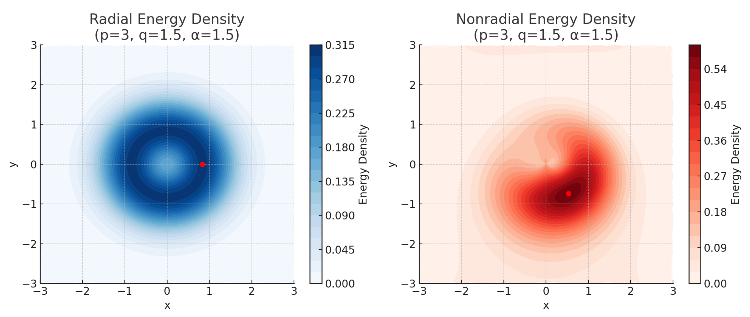
Before proceeding with the proof of Theorem 4, we provide a visual representation of the symmetry-breaking phenomenon and the relevant parameter space.

Figure 3 visually highlights the transition from a radially symmetric solution to a nonradially symmetric one, illustrating the core idea of symmetry-breaking that will be formalized in Theorem 4.

Figure 4 reveals the critical regions for the existence and stability of ground-state solutions in the fractional nonlocal Schrödinger–Poisson–Slater equation. Specifically, the green dashed line marks the critical value for q beyond which solutions become unstable, while the orange and red lines delineate the bounds for the exponent p, indicating the regions where different types of solutions exist. The area between the orange and red lines (shown in yellow) is where nonradial solutions are stable, according to Theorem 4.

Proof of Theorem 4. 

First, we assume that the equation conserves both the mass

$$M\left(u\left(t\right)\right)={\int }_{{\mathbb{R}}^N}{\left|u(x,t)\right|}^{2}dx=M\left(u_0\right)=m_0,$$

and the energy

$$E\left(u\left(t\right)\right)={\displaystyle \frac{1}{2}}{\int }_{{\mathbb{R}}^N}\left({|\nabla u|}^2+{\left|u\right|}^2\right)dx+{\displaystyle \frac{\lambda }{2q}}{\int \int }_{{\mathbb{R}}^N\times {\mathbb{R}}^N}{\displaystyle \frac{{\left|u\left(x\right)\right|}^q{\left|u\left(y\right)\right|}^q}{{|x-y|}^{N-\alpha }}}dxdy-{\displaystyle \frac{1}{p}}{\int }_{{\mathbb{R}}^N}{\left|u\right|}^{p}dx.$$

We consider the minimization problem on the set

$${\Sigma }_{m_0}=\left\{u\in {\mathcal{E}}_{\alpha ,q}\cap H^1\left({\mathbb{R}}^N\right):M\left(u\right)=m_0\right\}.$$

□

• Step 1:  Coercivity of the Energy Functional

Now, we claim that, under our assumptions on p and q (5), the energy $E\left(u\right)$ is coercive. Indeed, on the one hand, by the Hardy–Littlewood–Sobolev inequality, there exists a constant $\widehat{C}>0$ such that

$${\displaystyle \frac{\lambda }{2q}}{\int }_{{\mathbb{R}}^N}\left(I_{\alpha }\ast {\left|u\right|}^q\right){\left|u\right|}^{q}dx\le {\displaystyle \frac{\lambda \widehat{C}}{2q}}C{\Vert \nabla u\Vert }_{L^2}^{2q{\theta }_1}.$$

where ${\theta }_1={\displaystyle \frac{N(q-2)+\alpha }{2q}}$ and $2-{\displaystyle \frac{\alpha }{N}}<q<{\displaystyle \frac{2N-\alpha }{N-2}}$. On the other hand, For the local term, by the Gagliardo–Nirenberg inequality, there exists a constant $C_p>0$ and an exponent ${\theta }_2\in (0,1)$ such that

$${\Vert u\Vert }_{L^p}\le C_p{\Vert \nabla u\Vert }_{L^2}^{{\theta }_2}{\Vert u\Vert }_{L^2}^{1-{\theta }_2}$$

Hence,

$${\int }_{{\mathbb{R}}^N}{\left|u\right|}^{p}dx\le C_p{\Vert u\Vert }_{L^p}^p\le C_p{\Vert \nabla u\Vert }_{L^2}^{p{\theta }_2}$$

where ${\theta }_2={\displaystyle \frac{N(p-2)}{2p}}$ and $p\in (2,2^{*})$. Above all, under our assumptions that ${\displaystyle \frac{4N-2\alpha +4q}{2N+2-\alpha }}<p<{\displaystyle \frac{2N}{N-2}}$, and $2-{\displaystyle \frac{\alpha }{N}}<q<{\displaystyle \frac{N+\alpha }{N-2}}$, we obtain

$$E\left(u\right)\ge {\delta \Vert u\Vert }_{H^1}^2-C,$$

(15)

for some $\delta >0$ and constant $C\ge 0$. Thus, the energy $E\left(u\right)$ is coercive and, being conserved, it controls the $H^1$ norm of the solution.

• Step 2: Existence of a Ground State via the Nehari Manifold

We now prove the existence of a ground-state solution by minimizing the energy functional over the Nehari manifold. The Nehari manifold is defined as

$$\mathcal{N}:=\left\{u\in {\mathcal{E}}_{\alpha ,q}\cap H^1\left({\mathbb{R}}^N\right):u\ne 0,N\left(u\right)=0\right\}$$

and we claim the following two properties:

Claim 1. 

The infimum of the energy functional over $\mathcal{N}$ is strictly positive, i.e., $d>0$. $d>0$.

For $u\in \mathcal{N}$,

$${\int |\nabla u|}^2+u^2+\lambda \int \int {\displaystyle \frac{{\left|u\left(x\right)\right|}^q{\left|u\left(y\right)\right|}^q}{{|x-y|}^{N-\alpha }}}={\int \left|u\right|}^p\le {\Vert u\Vert }_{H^1}^p.$$

It implies that

$$0<c_1{\Vert u\Vert }_{H^1}^2\le {\epsilon }_1{\Vert u\Vert }_{H^1}^{p}i.e.{\Vert u\Vert }_{H^1}\ge c^{{\displaystyle \frac{1}{p-2}}}.$$

Then, we obtain

$$\begin{array}{cc}\hfill E\left(u\right)& =\left({\displaystyle \frac{1}{2}}-{\displaystyle \frac{1}{p}}\right)\int {|\nabla u|}^2+u^2+\left({\displaystyle \frac{\lambda }{2q}}-{\displaystyle \frac{\lambda }{p}}\right)\int \int {\displaystyle \frac{{\left|u\left(x\right)\right|}^q{\left|u\left(y\right)\right|}^q}{{|x-y|}^{N-\alpha }}}\hfill \\ & ⩾\left({\displaystyle \frac{1}{2}}-{\displaystyle \frac{1}{p}}\right)c^{{\displaystyle \frac{2}{p-2}}}>0.\hfill \end{array}$$

Hence

$$d=\underset{u\in \mathcal{N}}{inf}E\left(u\right)>0.$$

Claim 2. 

There exists a function $u\in \mathcal{N}$ such that $d=E\left(u\right)$, meaning that u minimizes the energy functional. There exists $u\in \mathcal{N}$, such that $d=E\left(u\right)$.

Take a minimizing sequence $\left(u_j\right)\subset \mathcal{N}$, $E\left(u_j\right)\to d$. By this way, we assume that $\Vert u_j{\Vert }_{H^1}\le c$ for some uniform constant $c>0$,

$$u_n\rightharpoonup u\mathrm{weakly}\mathrm{in}{H}^1\left({\mathbb{R}}^N\right),$$

$$u_n\to u\mathrm{a}.\mathrm{e}.\mathrm{in}{\mathbb{R}}^N,$$

$$u_n\to u\mathrm{in}{L}_{\mathrm{loc}}^p\left({\mathbb{R}}^N\right)\mathrm{for}p<{\displaystyle \frac{2N}{N-2}}.$$

For the nonlocal term, the Hardy–Littlewood–Sobolev inequality yields

$${\int \int }_{{\mathbb{R}}^N\times {\mathbb{R}}^N}{\displaystyle \frac{{\left|u\left(x\right)\right|}^q{\left|u\left(y\right)\right|}^q}{{|x-y|}^{N-\alpha }}}dxdy\le C{\Vert u\Vert }_{L^s}^{2q},s={\displaystyle \frac{2Nq}{N+\alpha }}.$$

Since $s<{\displaystyle \frac{2N}{N-2}}$ when $q<{\displaystyle \frac{N+\alpha }{N-2}}$, applying the Sobolev embedding $H^1\left({\mathbb{R}}^N\right)\hookrightarrow L^s\left({\mathbb{R}}^N\right)$, we obtain

$${\Vert u\Vert }_{L^s}\le C{\Vert u\Vert }_{H^1},$$

and so

$$\int \int {\displaystyle \frac{{\left|u\right|}^q{\left|u\right|}^q}{{|x-y|}^{N-\alpha }}}\le C{\Vert u\Vert }_{H^1}^{2q}.$$

By the variational characterization of ${\lambda }_0$,

$${\lambda }_0=\underset{u\in H^1\left({\mathbb{R}}^N\right)\setminus \left\{0\right\}}{inf}{\displaystyle \frac{2q}{p}}{\displaystyle \frac{{\int \left|u\right|}^p}{\int \int \frac{{\left|u\right|}^q{\left|u\right|}^q}{{|x-y|}^{N-\alpha }}}},$$

for $\lambda \ge {\lambda }_0$, we obtain

$$\lambda \int \int {\displaystyle \frac{{\left|u\right|}^q{\left|u\right|}^q}{{|x-y|}^{N-\alpha }}}\ge {\Vert u\Vert }_{L^p}^p-{\Vert u\Vert }_{H^1}^2.$$

Hence, for $\lambda \ge {\lambda }_0$, the energy $E\left(u\right)$ is nonnegative.

According to the nonlocal Brezis–Lieb lemma [19], we know that

$$\underset{n\to \infty }{lim\; inf}\int \int {\displaystyle \frac{|u_n{|}^q{\left|u_n\right|}^q}{{|x-y|}^{N-\alpha }}}\ge \int \int {\displaystyle \frac{{\left|u\right|}^q{\left|u\right|}^q}{{|x-y|}^{N-\alpha }}}+\underset{n\to \infty }{lim\; inf}\int \int {\displaystyle \frac{|u_n{-u|}^q{|u_n-u|}^q}{{|x-y|}^{N-\alpha }}}.$$

By Proposition 4.3 and Proposition 3.3 in [19], equality in the nonlocal Brezis–Lieb inequality holds if $u_n\to u$ in $L_{\mathrm{loc}}^p\left({\mathbb{R}}^N\right)$ for $p>q$. Here, by Rellich–Kondrachov theorem, it is satisfied when ${\displaystyle \frac{1}{p}}>{\left({\displaystyle \frac{1}{2}}-{\displaystyle \frac{1}{\alpha }}\right)}_{+}$. Thus, we conclude that

$$\underset{n\to \infty }{lim}\int \int {\displaystyle \frac{|u_n{-u|}^q{|u_n-u|}^q}{{|x-y|}^{N-\alpha }}}=0.$$

Using the Sobolev embedding $H^1\left({\mathbb{R}}^N\right)\hookrightarrow L^s\left({\mathbb{R}}^N\right)$ again, we have

$$u_n\to u\mathrm{strongly}\mathrm{in}{H}^1\left({\mathbb{R}}^N\right).$$

Then, we deduce

$$N\left(u\right)\le lim\; inf\int |\nabla u_n{|}^2+u_n^2+\lambda \int \int {\displaystyle \frac{|u_n{\left(x\right)|}^q{\left|u_n\left(y\right)\right|}^q}{{|x-y|}^{N-\alpha }}}-\int {\left|u_n\right|}^p=0.$$

By contradiction, if $N\left(u\right)<0$, and

$$N\left(tu\right)=t^2\left({\int |\nabla u|}^2+{\epsilon }^2{u}^2\right)+\lambda t^{2q}\int \int {\displaystyle \frac{{\left|u\left(x\right)\right|}^q{\left|u\left(y\right)\right|}^q}{{|x-y|}^{N-d}}}-t^p\int {\left|u\right|}^p>0,$$

for $t>0$ small, then we have $N\left(t_{c}u\right)=0$ for some $0<t<1$. Then, $t_{c}u\in \mathcal{N}$ and $E\left(t_{c}u\right)⩾d$. But we compute:

$$d\le E\left(t_{c}u\right)=\left({\displaystyle \frac{1}{2}}-{\displaystyle \frac{1}{p}}\right)t_c^2{\Vert u\Vert }_{H^1}^2+\left({\displaystyle \frac{\lambda }{2q}}-{\displaystyle \frac{\lambda }{p}}\right)t_c^p\int {\left|u\right|}^p<E\left(u\right)=d,$$

which is absurd. Then, $N\left(u\right)=0$, $E\left(u\right)=d$, i.e., u is a minimizer of E on $\mathcal{N}$. Following the Lagrange multiplier, $E^{\prime }\left(u\right)v=\tilde{\lambda }{N}^{\prime }\left(u\right)v$, and taking $u=v$,

$$N\left(u\right)=E^{\prime }\left(u\right)u=\tilde{\lambda }{N}^{\prime }\left(u\right)u=0.$$

that is

$$\tilde{\lambda }\left({2\int |\nabla u|}^2+u^2+2q\lambda \int \int {\displaystyle \frac{{\left|u\left(x\right)\right|}^q{\left|u\left(y\right)\right|}^q}{{|x-y|}^{N-\alpha }}}-p\int {\left|u\right|}^p\right)=0.$$

It implies that

$$\tilde{\lambda }\left[{(2-p)\Vert u\Vert }_{H^1}^2+\lambda (2q-p)\int \int {\displaystyle \frac{{\left|u\left(x\right)\right|}^q{\left|u\left(y\right)\right|}^q}{{|x-y|}^{N-\alpha }}}\right]=0.$$

As we know $p>2$, $2q>p$ and $\lambda >0$, $u\ne 0$, we obtain $\tilde{\lambda }=0$. Therefore, we obtain $E^{\prime }\left(u\right)u=\tilde{\lambda }{N}^{\prime }\left(u\right)u=0$ for all $v\in H^1\left({\mathbb{R}}^N\right)$. Hence, u is a critical point. Then, $\varphi$ is a ground state.

• Step 3: Existence of Solutions to the Cauchy Problem

Consider the Cauchy problem

$$\left\{\begin{array}{c}i{\partial }_{t}u=-\Delta u+u+\lambda \left(I_{\alpha }\ast {\left|u\right|}^q\right){\left|u\right|}^{q-2}u-{\left|u\right|}^{p-2}u,(x,t)\in {\mathbb{R}}^N\times \mathbb{R},\hfill \\ u\left(0\right)=u_0\in H^1\left({\mathbb{R}}^N\right).\hfill \end{array}\right.$$

Define the linear operator

$$L=-\Delta +{\epsilon }^2.$$

Write the equation in Duhamel form, we have

$$u\left(t\right)=e^{itL}{u}_0-i{\int }_0^t{e}^{i(t-s)L}S\left(u\left(s\right)\right)ds,$$

where

$$S\left(u\right)=\lambda \left(I_{\alpha }\ast {\left|u\right|}^q\right){\left|u\right|}^{q-2}u-{\left|u\right|}^{p-2}u.$$

Fix $T>0$ and define

$$X_T:=C\left([0,T];H^1\left({\mathbb{R}}^N\right)\right)\cap S_T$$

where

$$S_T=L^{q_0}\left(0,T;W^{1,r_0}\left({\mathbb{R}}^N\right)\right)$$

and we choose the Schrödinger-admissible pair $(q_0,r_0)$

$$r_0={\displaystyle \frac{2Nq}{2N-\alpha }}\mathrm{and}{q}_0={\displaystyle \frac{4q}{Nq-2N+\alpha }}.$$

It follows from the classical Strichartz estimates, that is

$${‖e^{itL}{u}_0‖}_{X_T}\le C{‖u_0‖}_{H^1}.$$

In order to balance the interplay between the nonlocal term and the local term, define $N_T=L^{{\tilde{q}}^{\prime }}(0,T;W^{1,{\tilde{r}}^{\prime }}\left({\mathbb{R}}^N\right))$ with dual exponents ${\tilde{q}}^{\prime }={\displaystyle \frac{q_0}{2q-1}}$ and ${\tilde{r}}^{\prime }={\displaystyle \frac{r_0}{2q-1}}$. By the Hardy–Littlewood–Sobolev inequality and Sobolev’s embedding, we obtain

$${‖\lambda \left(I_{\alpha }\ast {\left|u\right|}^q\right){\left|u\right|}^{q-2}u‖}_{N_T}\le C{\Vert u\Vert }_{X_T}^{2q-1},$$

and using Sobolev’s embedding,

$${‖{\left|u\right|}^{p-2}u‖}_{N_T}\le C{\Vert u\Vert }_{X_T}^{p-1}.$$

hence, the Duhamel operator is bounded. This implies that

$$u\mapsto \left(I_{\alpha }\ast {\left|u\right|}^q\right){\left|u\right|}^{q-2}u$$

is locally Lipschitz from $X_T$ into the dual space $N_T$.

$${\Vert S\left(u\right)\Vert }_{N_T}\le C_R{\Vert u\Vert }_{X_T}^{2q-1},$$

where $C_R$. Thus, the overall estimate for the inhomogeneous term becomes

$${‖{\int }_0^t{e}^{i(t-s)L}S\left(u\left(s\right)\right)ds‖}_{S_T}\le C_R{\Vert u\Vert }_{X_T}^{2q-1},$$

where $T^{\eta }$ is time integration.

Above all, we obtain

$${\Vert \Phi \left(u\right)\Vert }_{X_T}\le C{‖u_0‖}_{H^1}+C{T}^{\eta }{C}_R{R}^{2q-1}.$$

here $\eta =1-{\displaystyle \frac{2q-1}{q_0}}=1-{\displaystyle \frac{(2q-1)(Nq-2N+\alpha )}{4q}}$. For any $u,v\in B_R$,

$$\Phi \left(u\right)\left(t\right)-\Phi \left(v\right)\left(t\right)=-i{\int }_0^t{e}^{i(t-s)L}(S\left(u\left(s\right)\right)-S\left(v\left(s\right)\right))ds$$

so

$$\begin{array}{cc}\hfill {\Vert \Phi \left(u\right)-\Phi \left(v\right)\Vert }_{X_T}& \le {C\Vert S\left(u\right)-S\left(v\right)\Vert }_{N_T}\hfill \\ & \le C{T}^{\eta }\left({\Vert u\Vert }_{X_T}^{2q-2}+{\Vert v\Vert }_{X_T}^{2q-2}+{\Vert u\Vert }_{X_T}^{p-2}+{\Vert v\Vert }_{X_T}^{p-2}\right){\Vert u-v\Vert }_{X_T}\hfill \\ & \le C{T}^{\eta }\left(4R^{2q-2}\right){\Vert u-v\Vert }_{X_T}.\hfill \end{array}$$

so the mapping

$$\Phi \left(u\right)\left(t\right)=e^{itL}{u}_0-i{\int }_0^t{e}^{i(t-s)L}S\left(u\left(s\right)\right)ds$$

is a contraction on a ball $B_R\subset X_T$, where

$$B_R=\left\{u\in X_T:{\Vert u\Vert }_{X_T}\le R\right\},$$

for some $R>0$ provided $T>0$ is sufficiently small. Thus, there exists a unique local solution $u\in X_T$. It implies that if the initial data have finite energy Then, the solution cannot blow up in finite time.

By the conservation of energy and mass, and the coercivity inequality (15),

$${\Vert u\left(t\right)\Vert }_{H^1}^2\le {\displaystyle \frac{E\left(u_0\right)+C}{\delta }},\forall t,$$

the local solution extends globally in time, i.e.,

$$u\in C\left(\mathbb{R};H^1\left({\mathbb{R}}^N\right)\right).$$

Moreover, the solution depends continuously on the initial data.

• Step 4: Orbital Stability of the Ground State

In the end, we prove orbital stability of the ground state. By contradiction, assume that orbital stability fails. Then, there exists an ${ϵ}_0>0$, a sequence of initial data $\left\{u_n^0\right\}\subset H^1\left({\mathbb{R}}^N\right)$, and a sequence of positive times $\left\{t_n\right\}$ such that

$${‖u_n^0-\varphi ‖}_{H^1}\to 0\mathrm{as}n\to \infty$$

but the corresponding solutions $u_n\left(t\right)$ of Equation (2) with initial data $u_n^0$ satisfy

$$\underset{\theta \in \mathbb{R}}{inf}{‖u_n\left(t_n\right)-e^{i\theta }\varphi ‖}_{H^1}>{ϵ}_0\mathrm{for}\mathrm{all}n$$

Denote ${\varphi }_n:=u_n\left(t_n\right)$. At time $t_n$, we have

$$E\left({\varphi }_n\right)\to m\left(m_0\right)\mathrm{and}M\left({\varphi }_n\right)\to M\left(Q\right).$$

Next, denote by $u_n^0$ the modulated initial data sequence. Since $\varphi$ is a ground state to (2), by definition, we have

$$E\left(\varphi \right)=m\left(m_0\right):=\underset{\begin{array}{c}u\ne 0\\ u\in H^1\end{array}}{inf}E\left(u\right)\mathrm{and}{\Vert \varphi \Vert }_{H^1}:=b>0.$$

By Sobolev embedding, we still have

$${‖u_n^0-Q‖}_{L^p}^p\le {‖u_n^0-Q‖}_{H^1}^p\to 0$$

so $u_n^0\to Q$ in $L^p$. Then, conservation laws imply that, up to translations and phase shifts,

$${‖{\varphi }_n-Q‖}_{H^1}\to 0.$$

In order to conclude strong convergence of the sequence, we must rule out vanishing and dichotomy in the concentration-compactness principle.

Rule out Vanishing. If the mass of ${\varphi }_n$ “spreads out” to infinity, then $E\left({\varphi }_n\right)$ would not converge to $m\left(m_0\right)$ contradicting energy conservation.

Assume vanishing, which means

$$\underset{n\to \infty }{lim}\underset{y\in {\mathbb{R}}^N}{sup}{\int }_{B(y,R)}{\left|{\varphi }_n\left(x\right)\right|}^{2}dx=0\forall R>0.$$

By Lions’ vanishing lemma [35], for $2<p<2^{*}$, ${lim}_{n\to \infty }{‖{\varphi }_n‖}_{L^p}=0$. The nonlocal term is controlled by the Hardy–Littlewood–Sobolev inequality (6):

$$\int \int {\displaystyle \frac{{\left|{\varphi }_n\left(x\right)\right|}^q{\left|{\varphi }_n\left(y\right)\right|}^q}{{|x-y|}^{N-\alpha }}}dxdy\le C{‖{\varphi }_n‖}_{L^s}^{2q},s={\displaystyle \frac{2Nq}{N+\alpha }}.$$

Since $s<2^{*}$ (from $q<{\displaystyle \frac{N+\alpha }{2N}}p$), vanishing implies ${‖{\varphi }_n‖}_{L^s}\to 0$, so

$$\int \int {\displaystyle \frac{{\left|{\varphi }_n\left(x\right)\right|}^q{\left|{\varphi }_n\left(y\right)\right|}^q}{{|x-y|}^{N-\alpha }}}dxdy\to 0.$$

Rule out Dichotomy. Let $m\left(m_0\right)$ denote the minimal energy among functions with fixed mass $m_0$, i.e.,

$$m\left(m_0\right)=inf\{E\left(u\right):u\in H^1\left({\mathbb{R}}^N\right),M\left(u\right)=m_0\},$$

where

$$E\left(u\right)={\displaystyle \frac{1}{2}}{\int }_{{\mathbb{R}}^N}\left({|\nabla u|}^2+{\left|u\right|}^2\right)dx+{\displaystyle \frac{\lambda }{2q}}{\int \int }_{{\mathbb{R}}^N\times {\mathbb{R}}^N}{\displaystyle \frac{{\left|u\left(x\right)\right|}^q{\left|u\left(y\right)\right|}^q}{{|x-y|}^{N-\alpha }}}dxdy-{\displaystyle \frac{1}{p}}{\int }_{{\mathbb{R}}^N}{\left|u\right|}^{p}dx,$$

and the mass is

$$M\left(u\right)={\int }_{{\mathbb{R}}^N}{\left|u\right|}^{2}dx.$$

Assume by contradiction that there exists a minimizing sequence $\left\{{\varphi }_n\right\}$ for $m\left(m_0\right)$, which exhibits dichotomy. That is, after extracting a subsequence, there exist sequences $v_n$ and $w_n$ with asymptotically disjoint supports such that

$$\Vert {\varphi }_n-(v_n+w_n){\Vert }_{H^1}\to 0,\Vert v_n{\Vert }_{L^2}^2\to \alpha ,{\Vert w_n\Vert }_{L^2}^2\to m_0-\alpha ,$$

for some $0<\alpha <m_0$. In this scenario, the splitting of ${\varphi }_n$ into two disjoint parts implies that the strict subadditivity of $m_{\lambda }$ is violated. Denote

$$A\left(u\right)={\displaystyle \frac{1}{2}}{\int }_{{\mathbb{R}}^N}\left({|\nabla u|}^2+{\left|u\right|}^2\right)dx;B\left(u\right)={\displaystyle \frac{\lambda }{2q}}{\int \int }_{{\mathbb{R}}^N\times {\mathbb{R}}^N}{\displaystyle \frac{{\left|u\left(x\right)\right|}^q{\left|u\left(y\right)\right|}^q}{{|x-y|}^{N-\alpha }}}dxdy;C\left(u\right)={\displaystyle \frac{1}{p}}{\int }_{{\mathbb{R}}^N}{\left|u\right|}^{p}dx;$$

Define the scaling

$$u_{\theta }\left(x\right)={\theta }^{a}u\left({\theta }^{b}x\right);\theta \in (1,+\infty ),$$

where $a={\displaystyle \frac{1}{2}}+{\displaystyle \frac{N-2}{2}}b={\displaystyle \frac{1+b(N-2)}{2}}$ and $b={\displaystyle \frac{1-q}{q(N-2)-(N+\alpha )}}$. Through direct computation, we obtain

$$E\left(u_{\theta }\right)={\theta }^{2a+2b-bN}A\left(u\right)+{\theta }^{2aq-b(N+\alpha )}B\left(u\right)-{\theta }^{ap-bN}C\left(u\right)=\theta A\left(u\right)+\theta B\left(u\right)-{\theta }^{s}C\left(u\right).$$

Under the parameter assumption, we deduce that

$$s={\displaystyle \frac{p}{2}}\left(1-{\displaystyle \frac{(2-N)(q-1)}{q(2-N)+(3N-\alpha )}}\right)-{\displaystyle \frac{N(q-1)}{q(2-N)+(3N-\alpha )}}>1.$$

By the definition of $m\left(m_0\right)$ and taking the infimum over all $u\in {\Sigma }_{m_0}$ yields

$$m\left(\theta \alpha \right)<\theta m\left(\alpha \right).$$

Here, we employ a key lemma in concentration-compactness from [12]. The lemma asserts that if a function $h:[0,m_0]\to \mathbb{R}$ satisfies

$$h\left(\theta \alpha \right)<\theta h\left(\alpha \right)\mathrm{for}\mathrm{all}\alpha \in (0,m_0)\mathrm{and}\theta \in \left(1,{\displaystyle \frac{m_0}{\alpha }}\right],$$

then it is strictly subadditive

$$h\left(m_0\right)<h\left(\alpha \right)+h(m_0-\alpha )\mathrm{for}\mathrm{all}\alpha \in (0,m_0).$$

The strict subadditivity assumption then reads

$$m\left(m_0\right)<m\left(\alpha \right)+m(m_0-\alpha )\mathrm{for}\mathrm{all}\alpha \in (0,m_0).$$

Since $\left\{{\varphi }_n\right\}$ is a minimizing sequence with $M\left({\varphi }_n\right)\to m_0$ and $E\left({\varphi }_n\right)\to m\left(m_0\right)$, one expects that if dichotomy occurs Then, the energy asymptotically splits as

$$E\left({\varphi }_n\right)=E\left(v_n\right)+E\left(w_n\right)+o\left(1\right).$$

By the definition of minimal energy, we have

$$E\left(v_n\right)\ge m\left(\Vert v_n{\Vert }_{L^2}^2\right)\mathrm{and}E\left(w_n\right)\ge m\left(\Vert w_n{\Vert }_{L^2}^2\right).$$

Passing to the limit, we obtain

$$\underset{n\to \infty }{lim\; inf}E\left({\varphi }_n\right)\ge m\left(\alpha \right)+m(m_0-\alpha ),$$

which contradicts the dichotomy.

Since neither vanishing nor dichotomy occurs, the concentration-compactness principle ensures that there exists a sequence $\left\{y_n\right\}\subset {\mathbb{R}}^N$ such that the translated sequence

$$v_n\left(x\right)={\varphi }_n\left(x+y_n\right)\to \varphi \mathrm{strongly}\mathrm{in}{H}^1\left({\mathbb{R}}^N\right).$$

Thus, $\varphi$ achieves the minimal energy $m\left(m_0\right)$ and is a ground state. Consequently, for large n,

$$\underset{\theta \in \mathbb{R},y\in {\mathbb{R}}^N}{inf}{‖u^n\left(t_n\right)-e^{i\theta }Q(·-y)‖}_{H^1}\to 0.$$

Thus, by ruling out vanishing and dichotomy and applying the concentration compactness principle, we conclude that the sequence $\left\{{\varphi }_n\right\}$ converges strongly in $H^1\left({\mathbb{R}}^N\right)$, and the ground-state solution is orbitally stable.

References

1. Adams, D.R.; Hedberg, L.I. Function Spaces and Potential Theory; Springer: Berlin/Heidelberg, Germany, 1999; Volume 314. [Google Scholar]
2. Moroz, V.; Van Schaftingen, J. Groundstates of nonlinear Choquard equations: Existence, qualitative properties and decay asymptotics. J. Funct. Anal. 2013, 265, 153–184. [Google Scholar] [CrossRef]
3. Di Nezza, E.; Palatucci, G.; Valdinoci, E. Hitchhiker’s guide to the fractional Sobolev spaces. Bull. Sci. Math. 2012, 136, 521–573. [Google Scholar] [CrossRef]
4. Slater, J.C. A simplification of the Hartree-Fock method. Phys. Rev. 1951, 81, 385. [Google Scholar] [CrossRef]
5. Bokanowski, O.; López, J.L.; Soler, J. On an exchange interaction model for quantum transport: The Schrödinger–Poisson–Slater system. Math. Model. Methods Appl. Sci. 2003, 13, 1397–1412. [Google Scholar] [CrossRef]
6. Mauser, N.J. The Schrödinger-Poisson-Xα equation. Appl. Math. Lett. 2001, 14, 759–763. [Google Scholar] [CrossRef]
7. Benguria, R.; Brézis, H.; Lieb, E.H. The Thomas-Fermi-von Weizsäcker theory of atoms and molecules. Commun. Math. Phys. 1981, 79, 167–180. [Google Scholar] [CrossRef]
8. Lieb, E.H. Thomas-Fermi and related theories of atoms and molecules. Rev. Mod. Phys. 1981, 53, 603. [Google Scholar] [CrossRef]
9. Eberhard, E.; Dreizler, R. Density Functional Theory: An Advanced Course; Springer: Berlin/Heidelberg, Germany, 2011. [Google Scholar]
10. Nier, F. A variational formulation of Schrödinger-Poisson systems in dimension d ≤ 3. Commun. Partial. Differ. Equ. 1993, 18, 1125–1147. [Google Scholar] [CrossRef]
11. Ruiz, D. The Schrödinger–Poisson equation under the effect of a nonlinear local term. J. Funct. Anal. 2006, 237, 655–674. [Google Scholar] [CrossRef]
12. Lions, P.L. The concentration-compactness principle in the calculus of variations. The limit case, part 1. Rev. Mat. Iberoam. 1985, 1, 145–201. [Google Scholar] [CrossRef]
13. Lieb, E.H.; Loss, M. Analysis; American Mathematical Society: Providence, RI, USA, 2001; Volume 14. [Google Scholar]
14. Lieb, E.H.; Simon, B. The Thomas-Fermi theory of atoms, molecules and solids. Adv. Math. 1977, 23, 22–116. [Google Scholar] [CrossRef]
15. Lions, P. The Choquard equation and related questions. Nonlinear Anal. Theory Methods Appl. 1980, 4, 1063–1072. [Google Scholar] [CrossRef]
16. Jeanjean, L.; Le, T.T. Multiple normalized solutions for a Sobolev critical Schrödinger-Poisson-Slater equation. J. Differ. Equations 2021, 303, 277–325. [Google Scholar] [CrossRef]
17. Berestycki, H.; Lions, P.L. Nonlinear scalar field equations. Pt. 1. Arch. Ration. Mech. Anal. 1983, 82, 313–346. [Google Scholar] [CrossRef]
18. Ruiz, D. On the Schrödinger-Poisson-Slater system: Behavior of minimizers, radial and nonradial cases. Arch. Ration. Mech. Anal. 2010, 198, 349–368. [Google Scholar] [CrossRef]
19. Mercuri, C.; Moroz, V.; Van Schaftingen, J. Groundstates and radial solutions to nonlinear Schrödinger–Poisson–Slater equations at the critical frequency. Calc. Var. Partial. Differ. Equations 2016, 55, 1–58. [Google Scholar] [CrossRef]
20. Bellazzini, J.; Ghimenti, M.; Mercuri, C.; Moroz, V.; Van Schaftingen, J. Sharp Gagliardo–Nirenberg inequalities in fractional Coulomb–Sobolev spaces. Trans. Am. Math. Soc. 2018, 370, 8285–8310. [Google Scholar] [CrossRef]
21. Servadei, R.; Valdinoci, E. Variational methods for non-local operators of elliptic type. Discret. Contin. Dyn. Syst 2013, 33, 2105–2137. [Google Scholar] [CrossRef]
22. Tang, Y.; Huang, Y.; Liu, Z.; Moroz, V. Symmetry breaking and multiple solutions for the Schrödinger–Poisson–Slater equation. Z. Angew. Math. Phys. 2024, 75, 114. [Google Scholar] [CrossRef]
23. Liu, Z.; Moroz, V. Asymptotic profile of ground states for the Schrödinger–Poisson–Slater equation. Nonlinear Anal. 2022, 218, 112778. [Google Scholar] [CrossRef]
24. Zhang, L.; Hou, W. Standing waves of nonlinear fractional p-Laplacian Schrödinger equation involving logarithmic nonlinearity. Appl. Math. Lett. 2020, 102, 106149. [Google Scholar] [CrossRef]
25. Wang, G.; Ren, X.; Bai, Z.; Hou, W. Radial symmetry of standing waves for nonlinear fractional Hardy–Schrödinger equation. Appl. Math. Lett. 2019, 96, 131–137. [Google Scholar] [CrossRef]
26. Zhang, L.; Ahmad, B.; Wang, G.; Ren, X. Radial symmetry of solution for fractional p- Laplacian system. Nonlinear Anal. 2020, 196, 111801. [Google Scholar] [CrossRef]
27. Zhang, L.; Liu, Q.; Ahmad, B.; Wang, G. Nonnegative solutions of a coupled k-Hessian system involving different fractional Laplacians. Fract. Calc. Appl. Anal. 2024, 27, 1835–1851. [Google Scholar] [CrossRef]
28. Zhang, L.; Nie, X. Hopf’s lemma and radial symmetry for the Logarithmic Laplacian problem. Fract. Calc. Appl. Anal. 2024, 27, 1906–1916. [Google Scholar] [CrossRef]
29. Wang, G.; Yang, R.; Zhang, L. The properties of a new fractional g-Laplacian Monge-Ampère operator and its applications. Adv. Nonlinear Anal. 2024, 13, 20240031. [Google Scholar] [CrossRef]
30. Siciliano, G. Multiple positive solutions for a Schrödinger–Poisson–Slater system. J. Math. Anal. Appl. 2010, 365, 288–299. [Google Scholar] [CrossRef]
31. Georgiev, V.; Prinari, F.; Visciglia, N. On the radiality of constrained minimizers to the Schrödinger–Poisson–Slater energy. Ann. L’Inst. Henri Poincaré Anal. Non Linéaire 2012, 29, 369–376. [Google Scholar] [CrossRef]
32. Lei, C.; Lei, Y. On the existence of ground states of an equation of Schrödinger–Poisson–Slater type. Comptes Rendus. Mathématique 2021, 359, 219–227. [Google Scholar] [CrossRef]
33. Lions, P.L. Solutions of Hartree-Fock equations for Coulomb systems. Commun. Math. Phys. 1987, 109, 33–97. [Google Scholar] [CrossRef]
34. Willem, M. Minimax Theorems; Springer: Berlin/Heidelberg, Germany, 2012; Volume 24. [Google Scholar]
35. Lions, P.L. The concentration-compactness principle in the Calculus of Variations. The locally compact case, part 1. Ann. L’Inst. Henri Poincaré Anal. Non Linéaire 1984, 1, 109–145. [Google Scholar] [CrossRef]
Figure 1. Three-dimensional (3D) energy functional E ( u ) landscape, illustrating the mountain pass geometry with critical points marked as red ‘×’, highlighting the transition between local minima and critical points.
Fractalfract 09 00329 g001
Figure 2. Radial ground-state profile u ( r ) for the stationary Schrödinger–Poisson–Slater Equation (2) with N = 3 , α = 1 , q = 2 , p = 4 and λ = 1 . The solution is obtained via an imaginary-time gradient-flow scheme on a radial mesh r [ 0 , 20 ] ( Δ r = 0.05 ). The curve is smooth at the origin ( u ( 0 ) = 0 ) and decays monotonically to zero.
Fractalfract 09 00329 g002
Figure 3. Symmetry-breaking comparison of ground states. (Left): Radial energy-density contour for N = 3 , α = 1.5 , p = 3.0 , q = 1.5 , λ = 0.5 . The red dot marks the minimizer in the radial subspace (perfectly circular symmetry). (Right): Nonradial energy-density contour under the same parameters, where the red dot indicates the global minimizer in the full space—evidently off the circle, illustrating symmetry-breaking.
Fractalfract 09 00329 g003
Figure 4. Parameter space for the existence and stability of ground-state solutions in the nonlocal Schrödinger–Poisson–Slater equation (Theorem 4) for N = 3 and α = 1 .
Fractalfract 09 00329 g004