Article

Personalised Fractional-Order Autotuner for the Maintenance Phase of Anaesthesia Using Sine-Tests

1
Department of Automation, Technical University of Cluj-Napoca, Memorandumului Street No 28, 400114 Cluj-Napoca, Romania
2
Research Group on Dynamical Systems and Control, Department of Electromechanics, Systems and Metal Engineering, Ghent University, Tech Lane Science Park 125, 9052 Gent, Belgium
*
Author to whom correspondence should be addressed.
Fractal Fract. 2025, 9(5), 317; https://doi.org/10.3390/fractalfract9050317
Submission received: 4 April 2025 / Revised: 6 May 2025 / Accepted: 13 May 2025 / Published: 15 May 2025
(This article belongs to the Special Issue Fractional Mathematical Modelling: Theory, Methods and Applications)

Abstract

The research field of clinical practice has experienced a substantial increase in the integration of information technology and control engineering, which includes the management of medication administration for general anaesthesia. The invasive nature of input signals is the reason why autotuning methods are not widely used in this research field. This study proposes a non-invasive method using small-amplitude sine tests to estimate patient parameters, which allows the design of a personalised controller using an autotuning principle. The primary objective is to regulate the Bispectral Index through the administration of Propofol during the maintenance phase of anaesthesia, using a personalised fractional-order PID. This work aims to demonstrate the effectiveness of personalised control, which is facilitated by the proposed sine-based method. The closed-loop simulation results demonstrate the efficiency of the proposed approach.

1. Introduction

Automated drug dosage systems integrate real-time physiological data, such as blood pressure, heart rate, oxygen saturation, and levels of exhaled carbon dioxide, utilising computerised algorithms designed to control the delivery of anaesthetic agents. Sensors continuously monitor these parameters, and the system’s algorithms adjust the rate of drug infusion to maintain a stable anaesthetic state that is neither too deep nor too light. Target-controlled infusion (TCI) systems are frequently implemented in general anaesthesia [1,2,3]. To obtain a specific target concentration of the anaesthetic agent in the blood or brain, these systems calculate the drug dose necessary.
The primary goal of research in automated systems for anaesthesia is to obtain precise control over the administration of drug dosage during all stages of a surgical procedure. This precision is crucial for ensuring the safety and well-being of patients, as severe complications can result from insufficient or excessive dosing [4]. Nevertheless, a closed-loop control system that is capable of continually adjusting drug delivery in response to the patient’s evolving physiological state is necessary to achieve such precision.
Anaesthesia mainly comprises three stages: the induction phase, the maintenance phase and the emergence phase [5]. The induction phase commences with the administration of intravenous anaesthetic agents, which rapidly induce unconsciousness in the patient. The maintenance phase aims to ensure that the patient remains unconscious and pain-free throughout the procedure, provided that the desired depth of anaesthesia has been achieved. This is accomplished by closely monitoring vital signs while administering a continuous intravenous infusion of anaesthetic medications. Ultimately, the patient’s consciousness is progressively restored during the emergence phase, as the administration of anaesthetic agents is reduced or ceased. Careful management during this stage provides a smooth recovery while reducing the likelihood of complications, including agitation, nausea, or pain. One of the most important aspects in anaesthesia is ensuring the depth of hypnosis, evaluated using the measured Bispectral Index (BIS) signal [6]. An adequate level of hypnosis is usually achieved by administering a certain Propofol drug dose at a certain rate. Several control strategies have been developed to handle Propofol drug dosing to achieve a specific BIS signal. Almost all control algorithms share a common requirement: the necessity of a mathematical model for the patient. Although the majority of research focuses on population-based models, a subset has shifted towards personalised control [7]. This results in tailored controller parameters based on patient demographics. The results of the closed-loop simulation indicate that the individualised controller enhances robustness to patient variability; however, it also demonstrates a reduction in bandwidth, leading to diminished disturbance rejection capabilities.
The primary objective of this research is to investigate the benefit of using personalised controllers, designed using autotuning methods. Such an approach has yet to be considered for anaesthesia regulation. The necessity of accurately predicting the patient response remains essential amid the development of autotuning mechanisms. Autotuners are dependent on feedback from the system they control, implying that if the system’s behaviour is not well predicted, the tuning process may be inaccurate, resulting in suboptimal or even unsafe outcomes [8]. Performing classical autotuning tests, such as relay tests or Ziegler–Nichols, is completely unfeasible due to safety reasons [9]. These tests require finding the critical operating point of a system. For example, causing the patient’s brain activity to experience a sustained oscillation regime having considerable amplitude is strongly against clinical safety standards. However, minimally invasive methods with small amplitude input signals would be acceptable. In this paper, such an approach is attempted, and it is based on a sine test that is compliant with patients’ safety standards and provides sufficient data for tuning the controller. The data collected using this sine test are further used to design fractional-order autotuners. The choice of fractional-order controllers is based on their enhanced flexibility and robustness compared to the traditional integer order controllers [10].
Fractional-order PID (FO-PID) controllers present advantages compared to traditional integer-order PID controllers in the context of general anaesthesia, especially in regulating the depth of hypnosis and maintaining hemodynamic stability. Research indicates that FO-PID controllers demonstrate improved robustness to patient variability, resulting in more consistent performance across varied patient populations [11]. They offer enhanced disturbance rejection, effectively reducing the influence of surgical stimuli and other disruptions. Their expanded set of tuning parameters enhances flexibility and precision in control design, making them suitable for adaptive strategies that can adjust in real time to changing patient dynamics.
Fuzzy-type controllers are also appropriate in applications where mathematical models are difficult or unfeasible to establish. Additionally, fuzzy controllers are increasingly recognised for their effectiveness in managing general anaesthesia, particularly in addressing the nonlinearities, uncertainties, and imprecise characteristics of physiological responses during surgical interventions. Fuzzy logic controllers differ from traditional controllers by employing a rule-based approach that simulates human reasoning, rendering them especially appropriate for the complex and variable dynamics inherent in anaesthesia [12]. However, fuzzy rules and membership functions need to be carefully defined. The complexity can potentially increase in the context of patient intra- and inter-variability. Due to this, in this paper, a personalised fractional-order controller is preferred.
For the induction phase, a PID controller will be used for all patients. This PID controller is designed using a nominal patient model by using standard frequency domain tuning methods. The gain crossover frequency is imposed as a performance criterion to ensure a certain settling time during the induction phase. Once the BIS signal reaches a steady state value ranging between 47.5 and 52.5, indicative of an adequate level of hypnosis, the proposed sine test is applied using a frequency that matches the gain crossover frequency utilised for the induction phase. The sine test is further used to estimate the gain, phase, and derivative of the phase for each patient. This information is later employed in the autotuning of a fractional-order controller to be used during the maintenance phase. The safety range of BIS values is between 40 and 60 [13], with a steady-state value ideally equal to 50. Surgical stimuli occurring during the maintenance phase will cause variations in the BIS signal. The proposed method attempts to limit this variation and ensure that the BIS signal remains within a ±5% range of the steady-state value during the maintenance phase. The proposed sine test is robust to noisy signals and provides accurate estimations of the patient’s gain, phase, and derivative of the phase. As such, it enables the design of a personalised fractional-order controller.
The primary contribution and novelty of this research are the introduction of a sine-test-based autotuning approach for the design of personalised fractional-order controllers that are intended to regulate the depth of hypnosis in anaesthesia. This strategy eliminates the necessity for invasive procedures or time-consuming modelling efforts by directly estimating patient-specific dynamics from data using the sine test, in contrast to traditional methods that rely on constructing detailed patient models. The proposed autotuning method is entirely non-invasive, carries no risk to the patient, and offers a considerable improvement in efficiency and adaptability. This is the first application of such a method in the context of closed-loop anaesthesia control. This work represents an advance in the development of automated and personalised anaesthetic systems by offering a computationally efficient, safe, robust to noise, and practicable alternative for customising anaesthesia delivery.
To mimic the dynamics of a patient, a novel patient simulator [14] will be used. To model the patient’s BIS signal as a function of the administered Propofol, pharmacokinetic (PK) and pharmacodynamic (PD) models are most frequently used [15,16,17], with parameters depending on the patient’s age, weight, height, and gender. These models depict the manner in which a drug interacts with the body. In general, a three-compartment PK model delineates the fast-acting compartment (blood) and two additional compartments that represent the slower-acting tissue volumes of muscle and fat. The effect site concentration is represented by the addition of a hypothetical compartment that represents the transport/mixing dynamics of the substance to the effect location. PD modelling is fundamentally based on the dose–response relationship, which seeks to explain the mechanism by which variations in drug dosage result in changes in the intensity of the drug’s effect. The relationship between drug concentration and effect is frequently nonlinear, as the effects of a drug become more potent as the concentration increases. Several PK-PD models exist. In this case, the Schnider PK model [18] is employed along with a Hill function that models the PD compartment.
Closed-loop simulation results are performed. Comparative results are presented utilising both the population-based controller and the personalised controller for each patient during the maintenance phase. This demonstrates the effectiveness of personalised control.
The paper is structured as follows. Section 2 presents the mathematical foundation, while Section 3 details the procedures and methods utilised. Simulation results are included in Section 4, while the last section contains the conclusions and proposes prospective routes for further study in the field.

2. Materials and Methods

2.1. Sine Test Method

As stated in the introduction, once the BIS signal has reached steady state, a sine test is performed based on the approach in [19]. A sinusoidal input signal of small amplitude and frequency equal to ωgc, denoted u(t), is applied as the Propofol drug rate. The term ‘small’ refers to an amplitude which is significantly smaller than the dosage used for the maintenance phase. The exact quantities will be provided in the following subchapter.
The patient’s behaviour (BIS level) with respect to Propofol is denoted with P(s) and assumed to be unknown. The sine test will estimate the patient frequency response denoted as P(), as indicated hereafter. To tune a suitable controller, the following patient’s frequency response information is required: the magnitude M, the phase ϕ and the derivative of the phase at the gain-crossover frequency. Computing the magnitude and phase using sine tests measurements is straightforward:
M = P ( j ω g c ) = A o A i ,
ϕ = P j ω g c = ω g c τ = ω g c t i t o ,
where Ai and Ao represent the amplitudes of the input and the output signals, respectively, and τ = (tito) represents the time shift between the input and the output signals.
The third parameter, , will be used in the controller design to ensure the iso-damping property (or the robustness to gain variations). The human body is arguably one of the most unpredictable systems and prone to variations in time; therefore, the need for robust controllers is self-explanatory [11,20]. Extracting the phase derivative from a single sine test is not obvious, nor trivial. Figure 1 provides the innovative method proposed by the authors of [19] to compute , based on the magnitudes and phases of two signals: the output y(t) and the output of the process derivative, denoted as ȳ(t).
The next part will demonstrate that the methodology depicted in Figure 1 effectively provides the process derivative signal. The output ȳ(t) of the process derivative can be computed as:
y ¯ t = x t t y ( t ) ,
where x(t) denotes the output of the process P(jω) when an input signal t*u(t) is applied at its input. The operator * denotes the convolution of two signals. The property of the Laplace transform regarding the derivative of a signal will be employed:
d F ( s ) d s = L { t f ( t ) } ,
where F s = L { f ( t ) } .
The other mathematical definition of the process derivative output, ȳ(t), refers to the exact meaning of this signal:
Y ¯ s = d P s d s U ( s ) ,
where Y ¯ s and U(s) are the Laplace transforms of signals ȳ(t) and u(t), respectively.
Starting from the definition of the signal x(t) given in the theorem hypothesis, the following relation holds:
X ( s ) = P ( s ) L { t u ( t ) } ,
where X(s) represents the Laplace transform of x(t). Employing (4), (6) can be rewritten as:
X s = P s d U s d s   .
The Laplace transform of the sinusoidal input signal u(t) is given by:
U s = A i ω g c s 2 + ω g c 2   .
The derivative of U(s) is computed as follows:
d U s d s = 2 s s 2 + ω g c 2   U ( s ) .
Utilising (9) in (7) leads to:
X s = P s d U s d s = 2 s s 2 + ω g c 2 P s U s = 2 s s 2 + ω g c 2 Y s .
Equation (10) demonstrates that the signal x(t) can be computed utilising the output signal, y(t). The derivative of the output signal in Laplace domain is computed as:
d Y s d s = d P s U ( s ) d s = d P s d s U s + d U s d s P s .
If one utilises (5) and (10) in (11), it leads to:
d Y s d s = Y ¯ s X s .
Applying the inverse Laplace transform to (12) demonstrates that the process derivative is achievable. This indicates the feasibility of the testing procedure outlined in Figure 1. The derivative of the process is indeed accessible without any mathematical differentiation being employed.
The modulus and phase of ȳ(t) are computed in the same manner as in (1) and (2):
M ¯ = A y ¯ A i ,
ϕ ¯ = ω g c τ y ¯ = ω g c ( t i t y ¯ ) ,
where M ¯ is the amplitude of the signal ȳ(t) and ϕ ¯ is the phase shift between ȳ(t) and u(t).
The frequency domain relation of the process derivative is given by:
d P j ω d ω ω = ω g c = M ¯ e j ϕ ¯   ,
By expanding both the left- and right-hand sides of (15) and complex numbers mathematical refinements, the equation becomes:
j d M d ω ω = ω g c + M d ϕ d ω ω = ω g c = M ¯   cos ϕ ¯ ϕ + j M ¯   sin ϕ ¯ ϕ .
Equating the real and imaginary parts of the two terms in (16) results in the mathematical expression of the process phase derivative:
d ϕ = d P j ω d ω ω = ω g c =   M M ¯ cos ϕ ¯ ϕ ,
The procedure is now complete. However, the proposed approach for estimating the frequency response slope based on filtering the output signal y(t) as indicated in Figure 1 is simple, but error-prone. This study utilises a patient simulator and not real clinical data. The measurement of BIS is derived from electroencephalographic (EEG) signals through spectral and bispectral analysis. BIS measurements are often affected by noise, which can compromise their reliability. Common sources of noise include electromyographic (EMG) activity, poor electrode contact, external electrical interference, and patient-specific variability in EEG responses. To mitigate these issues, another approach that is robust to noise is presented in Appendix A.

2.2. Autotuning Mathematical Background

Upon obtaining the necessary parameters, ωgc, M, ϕ and (using (1), (2) and (17)), one may proceed with computing the controller parameters. Two types of fractional-order controllers are presented in this paper: FO-PI and FO-PID. Their transfer functions are indicated below:
H F O P I s = k p 1 + k i s μ ,
H F O P I D s = k p 1 + k i s μ + k d s λ ,
where µ and λ denote the fractional orders, while kp, ki, kd correspond to the proportional, integrative and derivative gains.
In this manuscript, the Grunwald–Letnikov [21] definition of the fractional-order derivative is used, which is generally preferred for applications, due to the convenient relation with the Laplace transform:
D α f ( t ) t = k h = lim h 0 1 h α j = 0 k 1 j α j f k h j h ,
where D α is the fractional derivative of order α . The mathematical formulas for the modulus, phase, and phase derivative of the controllers can be quickly deduced due to the known structure of these controllers. These equations are presented in [21].
An algorithm has been developed to compute the controller parameters. The tuning is performed according to a set of constraints. The gain crossover frequency is correlated to the settling time requirements. Higher values of ωgc are associated with quicker settling times. This is mathematically represented by the equation for magnitude:
H O L ( j ω g c ) = H F O - P I / D j ω g c P j ω g c = 1 ,
where H O L ( j ω g c ) = H F O - P I / D j ω g c P j ω g c is the open loop frequency response at ω g c . Phase margin (PM) serves as an essential performance metric associated with the stability of closed-loop systems, directly influencing the anticipated overshoot and undershoot. A high numerical value typically signifies a reduced excess. The equation that addresses the overshoot requirement is as follows:
H O L j ω g c = H F O - P I / D j ω g c + P j ω g c = π + P M ,
A robustness constraint has been added to address potential gain errors arising from patient variability:
d H O L j ω d ω ω = ω g c = 0 d P j ω d ω ω = ω g c + d H F O P I / D j ω d ω ω = ω g c = 0
Several other researchers [22,23] proposed supplementary performance criteria to be used in the design of fractional-order controllers, such as the sensitivity (S), and the complementary sensitivity (T) functions, to address the rejection of disturbances, among others. Nevertheless, a model of the process is necessary for all these performance criteria. No patient model is employed in this research, as the proposed control method is an autotuning algorithm. Therefore, only the performance specifications mentioned above (21)–(23) are used in the design of the controllers.
Several performance metrics are used to evaluate the efficiency of the proposed control algorithms. These correspond to the metrics usually employed in anaesthesia control and are detailed below.
Both the control signal and the output must exhibit stable behaviour with minimum oscillation. A high overshoot value presents a serious risk of taking the BIS out of the safe range. A large PM value is selected to ensure that a small overshoot is obtained:
σ 5 % .
Another important performance indicator is the time-to-target (TT), which refers to the time required for the controller to adjust the BIS signal to a desired range of values while adhering to the input safety constraints. The literature presents a range between 3 and 5 min as being appropriate for TT [24]. The condition imposed by the authors is:
T T 200   s .
An important aspect to be considered is that this constraint refers to the fast rejection of the disturbances and not to the response of the closed-loop system to a BIS reference. The BIS signal must stay within a range of 40 to 60 at all times, as stated in [13]; however, in this research, the values were restricted to 47.5 and 52.5 in order to have more precise control. Usually, a variation of ±10% is commonly employed for the Bispectral Index control. This research proposes a stricter range of only ±5%, with respect to the ideal BIS signal value of 50. This facilitates a more precise control and a safer clinical procedure.
The Propofol rate should not exceed 200 mg/kg/h [25], a value which corresponds to 3.33 mg/kg/min. The authors proposed an even stricter limitation of a maximum of 2.5 mg/kg/min. Thus, the control signal must always be positive and less than the imposed value due to safety concerns.
A third performance indicator used in this manuscript is the Integral of Absolute Error (IAE) to evaluate the efficiency of the controllers in rejecting disturbances, defined as:
IAE = 0 r ( t ) - B I S ( t ) dt ,
where BIS(t) is the simulated output and r(t) is the reference value.
The frequency response of the FO-PID controller is mathematically defined as:
H F O P I D j ω = k p ( 1 + k i j ω μ cos μ π 2 j   sin μ π 2 + k d ω λ cos λ π 2 + j   sin λ π 2 ) ,
Replacing (27) into (21)–(23), leads to the following system of nonlinear equations:
k p 1 + k i ω g c μ cos μ π 2 + k d ω g c λ cos λ π 2 2 + k i ω g c μ sin μ π 2 + k d ω g c λ sin λ π 2 2 1 P j ω gc = 0 ,
k i ω g c μ sin μ π 2 + k d ω g c λ sin λ π 2 1 + k i ω g c μ cos μ π 2 + k d ω g c λ cos λ π 2 tan π + P M - P j ω gc = 0 ,
ω g c μ 1 k i μ   sin μ π 2 + k d k i μ ω gc μ   sin μ + λ π 2 + k d k i λ ω gc λ   sin μ + λ π 2 + k d μ ω gc μ + λ   sin λ π 2 ω gc 2 μ + k i 2 + k d 2 ω gc 2 ( μ + λ ) + 2 k i ω gc μ   cos μ π 2 + 2 k d ω gc 2 μ + λ   cos λ π 2 + 2 k d k i ω gc λ + μ   cos μ + λ π 2 + d P j ω d ω ω = ω gc = 0 .

2.3. Algorithm Description
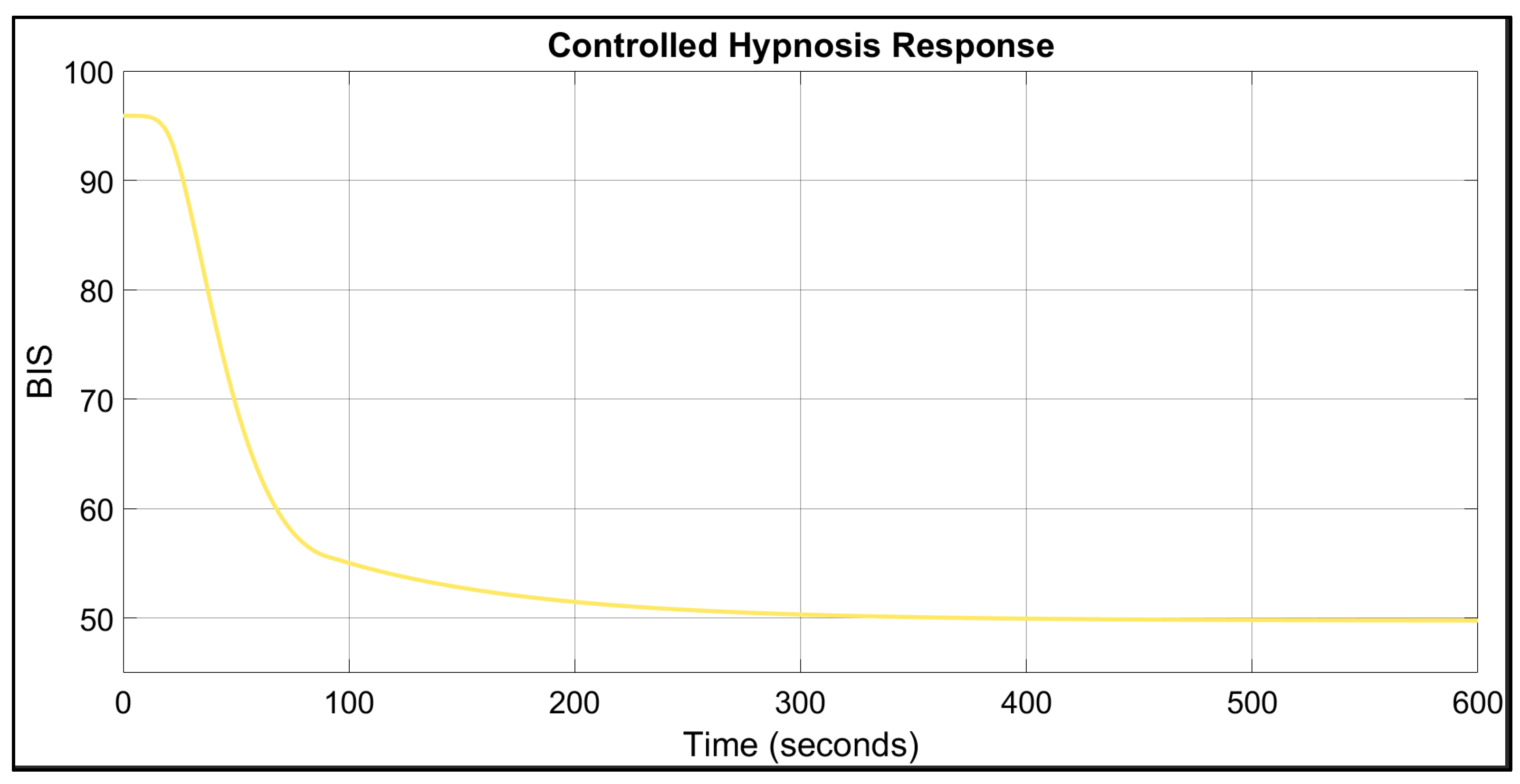
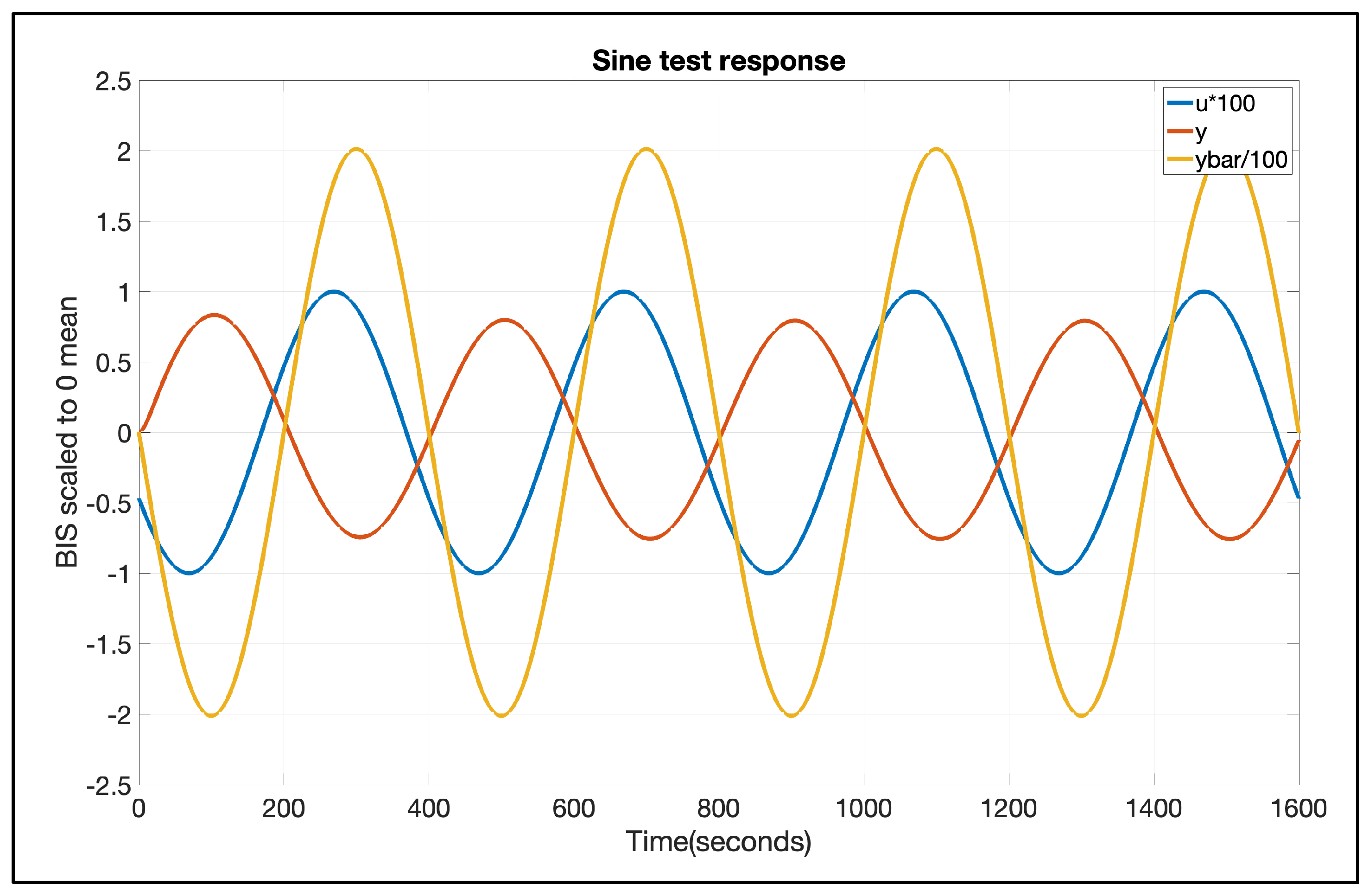
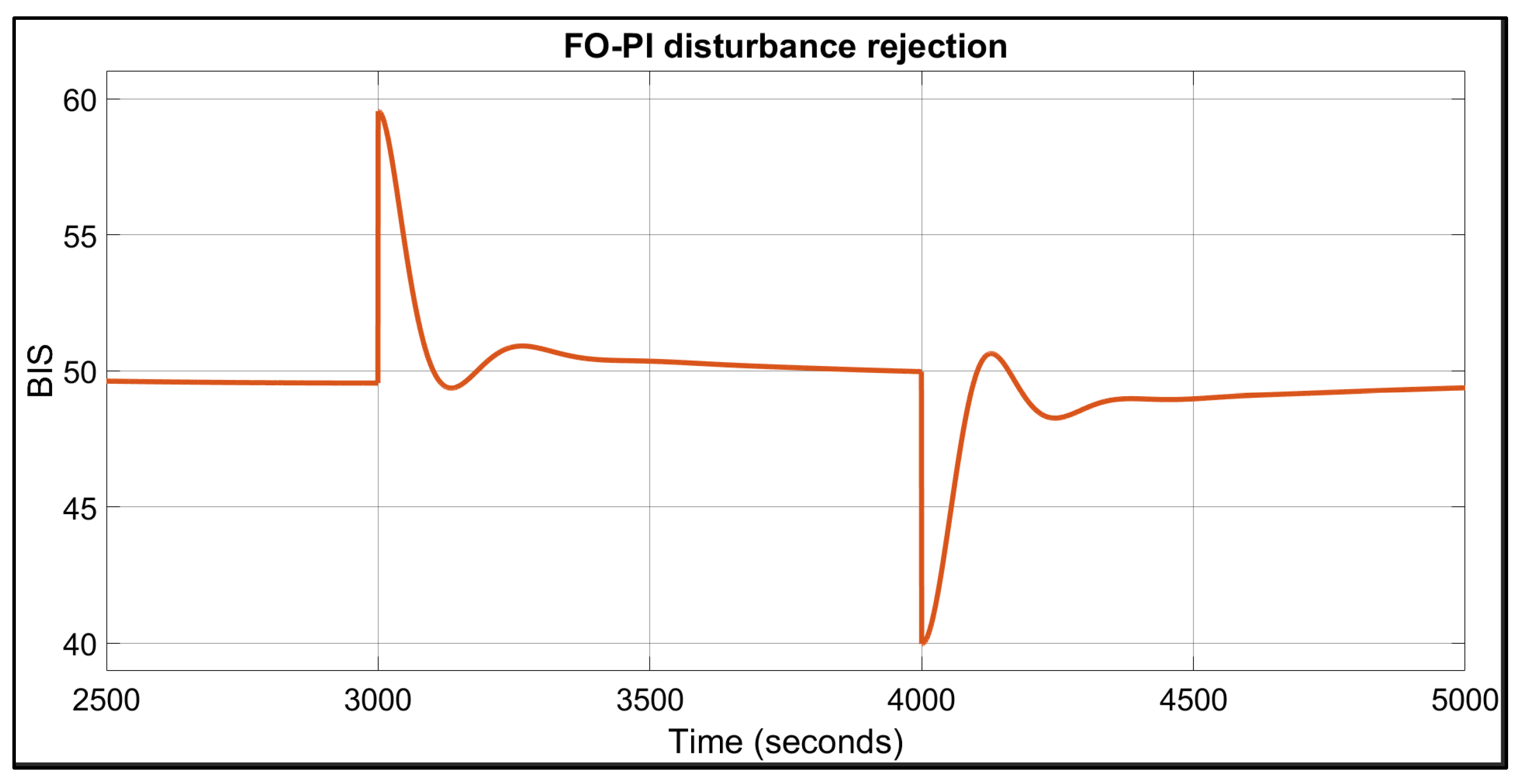
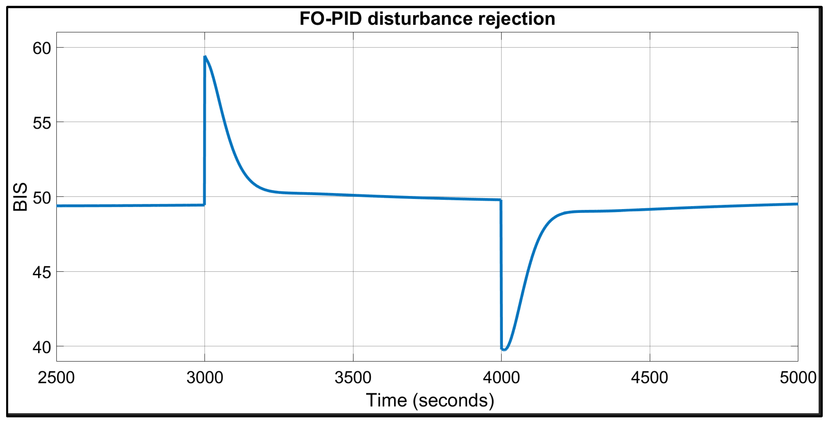
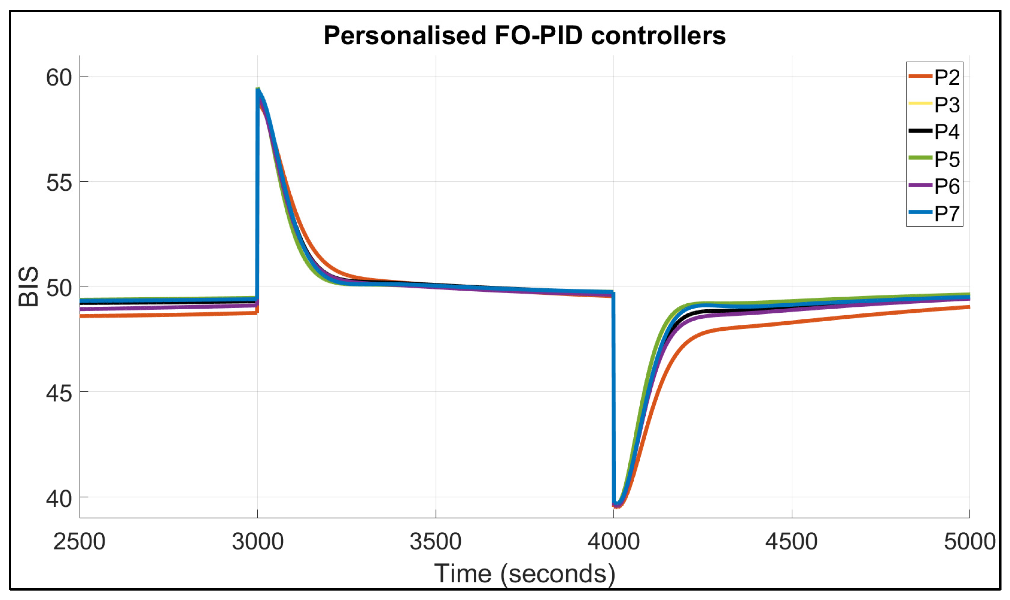
The procedure to design the personalised controllers is detailed in what follows. To determine all controller parameters, an optimisation algorithm based on the Matlab R2024A “fmincon” function is used to solve the system of equations composed of (28)–(30). For the tuning of the FO-PI controller parameters, only three parameters are estimated, namely the three controller parameters, kp, ki and µ. The remaining two parameters, kd and λ in (26)–(28), are set to null. For the FO-PID, all five parameters are estimated based on solving the system of equations in (28)–(30). The gain crossover frequency and the phase margin are specified a priori as design criteria, while an initial starting guess is provided for all controller parameters in the “fmincon” function. These initial values are those reported in [11].
First, an integer order PID controller will be computed for the induction phase, based on the already existing PK-PD model of the patient, with the model parameters estimated according to patient biometric data, such as height, weight, age, and sex [26]. This part will be only briefly presented since the focus of this paper is not on the induction phase. The authors studied the control of induction in [27]. The purpose of this step is to establish the cutting frequency, ωgc, which is later used for the sine test.
One relevant example of a PID autotuning algorithm can be found in [28]. Our adaptation of this algorithm provided a PID controller having the form:
H P I D = 0.205 1 + 0.00046 s + 82.5 s 1.66 s + 1 .
The imposed cutting frequency for this PID controller is 0.0025 rad/s. This finding is consistent with the current state of knowledge in the field of anaesthesia control, which posits that patients’ responses to these medications are slow [29]. The closed-loop response for one patient is presented in Figure 2.
As depicted in the picture above, there is a slight undershoot, and the TT is around 150 s, which is consistent with clinical protocols. This controller does not represent the main focus of this research, but merely a starting point.
The sine test will be applied to determine the patient’s parameters in the next step. The sine input has a frequency equal to 0.0025 rad/s and a 0.05 amplitude of Prop. The usual dosage for maintenance is around 0.1–0.2 mg/kg/min; therefore, the sine test is minimally invasive and does not affect the sleep state of the patient. Figure 3 presents the sinusoidal signals: u, y, and ȳ. Since there is a significant difference in amplitude for these signals, a scaling operation was necessary to improve the visibility and relevancy of the picture. After computations are performed according to (1), (2) and (17), the process parameters of the studied patient are: M = 39.47, ϕ = −104.85° and = −175.83.
Research suggests that better control can be achieved using separate controllers for the induction and maintenance phases [30]. In fact, the controller parameters must be precisely chosen to ensure that a rapid transient response without an excessive overshoot is achieved during the induction phase, while in the maintenance phase, the BIS values are kept within the specified interval. Even though a PK-PD model can be estimated a priori, patient uncertainties are prevalent, and the control strategy is susceptible to inter- and intra-patient variability. The retuning of the controller immediately following the induction phase using the BIS signal of each patient diminishes the amount of patient uncertainties and could potentially lead to better and personalised control over the maintenance phase. Once the patient’s frequency response characteristics are determined using the sine test, the FO-PI parameters will be computed using the described optimisation algorithm. Different FO-PI controllers can be obtained by imposing different ωgc and PM constraints. The proposed optimisation algorithm is also used for the tuning of the FO-PID parameters. The obtained controllers and their closed-loop simulations are detailed in the next section.
Remark 1.
The primary reason for considering the sine test to extract relevant patient frequency response characteristics is the assumption that the system is linear. The proposed analysis is conducted within a stable operating point. In this regime, the PD model effectively reduces to a simple gain, thereby rendering any inherent nonlinearities negligible. While it is true that the process exhibits nonlinear behaviour in general, the chosen steady state operating point allows for a linear approximation with sufficient accuracy. Additionally, in the maintenance phase, where BIS is close to 50, the system behaviour aligns well with linear assumptions. This stability ensures that nonlinear effects do not significantly influence the proposed methodology. As a result, the system can be reliably treated as linear without compromising the validity of the proposed approach.

3. Results

The performance of the controllers in rejecting disturbances will be analysed throughout this section. All presented results are specific to one patient, who was arbitrarily chosen to be the nominal patient. The characteristics of this patient are: age = 62 years, height = 168 cm, weight = 88 kg, sex = female. Proving the effectiveness of personalised control will be performed by using the controllers designed for the nominal case on other patients, followed by designing personalised controllers for each patient specifically. The results will prove the success of personalised control.
The parameters of the FO-PI tuned for the nominal patient are: kp = 0.0247, ki = 0.00059, µ = 1.1, and the structure of the controller is provided in (18). The imposed constraints were: ωgc = 0.0025 rad/s, PM = 50° and the iso-damping property. Figure 4 illustrates the disturbance rejection performance of this controller. Figure 5 presents the control signal, which verifies the clinical limitations of Propofol infusion.
The disturbance signal is composed of two step signals of amplitude 10, which occur consecutively with a 16-minute delay between them. This disturbance profile is supported by the literature [31]. This stimulus profile, or disturbance profile, simulates the patient’s arousal reflexes during a surgical procedure [32]. As depicted in the figure, the first disturbance is rejected in 67 s (close to 1 min) while the second disturbance is rejected in 74 s (less than 2 min). These performances are in accordance with the clinical standards. The control signal is within the limitations for safe anaesthetic procedures since its values are positive and smaller than 2.5 mg/kg/min. The range of the control signal is between 0 and 0.5 mg/kg/min, which indicates a higher safety level for the patient. The final performance metric, the IAE, has a value of 2137. While this may initially appear high, it is important to note that the integral is computed over a duration of 2500 s.
As for the FO-PID controller, the parameters are: kp = 0.02, ki = 0.0004, kd = 53.8, µ = 1.1, λ = 1.1. Figure 6 illustrates the disturbance rejection performance, with TT values of 109 and 134 s. While these values are slightly higher than those of the FO-PI controller, the response is smoother and exhibits no overshoot. The IAE is equal to 2431, which is slightly larger than the one obtained using the FO-PI controller.
The controller designed for the nominal patient is now used on different patients, and the disturbance rejection performances are analysed. One figure will be presented to illustrate the incapacity of one controller to fully compensate for inter-patient variability. Figure 7 shows that the initial FO-PI controller does not reject, according to clinical standards, the same disturbance profile when applied to another patient.
As shown in Figure 7, the BIS signal exhibits a highly oscillatory behaviour, which could be unpleasant or even harmful for the patient. The TT performance is approximately 180 s, which is nearly three times longer than in the nominal case. The final performance indicator, the IAE, is 5542, which is more than twice the value observed in the nominal case, further emphasising the need for personalised control strategies. The patient’s characteristics were: age = 50 years, height = 186 cm, weight = 96 kg, sex = male. The FO-PID response had worse performance due to the derivative component, which is more sensitive to variations in the parameters.

4. Discussion

The two initial controllers were applied to five more different patients, and the disturbance rejection performances did not comply with clinical standards. Longer TT, higher oscillations, and BIS levels not being kept within the 47.5–52.5 safe operating range were the drawbacks encountered. This finding strongly argues for the implementation of personalised control.
To design the personalised controllers, once the induction phase has been completed, a sine test similar to the one presented in Figure 3 is performed for each patient. The M, ϕ and parameters are obtained for each patient, and personalised FO-PI and FO-PID controllers are designed according to the proposed approach detailed in Section 2. Closed-loop simulations were performed for seven patients. The performances of the personalised controllers are presented in Table 1. Patient 1 is the nominal patient, and it serves as a reference. The two values for TT performance correspond to the response of the system to the chosen disturbance profile. The first value corresponds to the positive disturbance rejection, while the second value refers to the rejection of the negative disturbance.
The results indicate that recovery from a positive BIS disturbance is easier for patients. The awakening of a patient, indicated by an increase in the BIS signal, can be managed more effectively than preventing a descent into dangerously deep levels of hypnosis. This finding aligns with the existing literature [33]. In control engineering, the control signal (Propofol rate) is consistently positive; therefore, an increase in the Propofol rate would reduce the BIS signal and counteract the positive disturbance. A negative control signal indicates the extraction of the anaesthetic substance from the blood, which is impractical. Consequently, this complicates the rejection of a negative disturbance, specifically a decrease in the BIS signal.
Figure 8 and Figure 9 provide the graphical visualisation of Table 1. The results of this research are according to the clinical procedures. The nominal patient was not included in these figures for increased readability, as it has already been included in Figure 4 and Figure 6. Both proposed structures for the fractional-order controllers proved efficient in maintaining the BIS level in the safe range and also provide fast disturbance rejection loops. The FO-PI controller proves to be faster than the FO-PID; however, the latter provides a smoother signal with no oscillations.
The findings presented in this research are compared with those documented in the literature [30,34]. These studies also proposed the use of personalised FO-PID controllers to optimise Propofol dosage during general anaesthesia. A key point to note is that none of the referenced papers utilise an autotuning method; instead, they rely on patient-specific models.
The TT performances of the FO-PI controllers average 80 s for both positive and negative disturbance steps. The FO-PID controllers present a mean value of 130 s for disturbance rejection. The same disturbance profile was utilised in [30], and the TT performances are around 120 s. Considering that the BIS range used to compute TT in this study was narrower (47.5–52.5) compared to the broader 45–55 range in prior work, the results achieved here demonstrate faster response times despite the stricter criteria. In terms of overshoot, the FO-PI controllers yield comparable performance to that reported in [30], while the FO-PID controllers provide smoother control responses. One advantage of the referenced study is its larger dataset of 13 patients, compared to 7 in the current work. Nevertheless, both studies rely on relatively small patient datasets, which underscores the continued relevance of the proposed research.
In the comparative analysis with the study presented in [34], the results are generally similar. That study introduces three versions of FO-PID controllers, each tuned based on different performance criteria. Their average TT values are 40 s for positive disturbances and 70 s for negative disturbances, which is faster than those observed in this research. However, the overshoot values reported in [34] are higher than those achieved in the current study. The IAE values reported in [34] range from 1531 to 2354, which are comparable to those obtained in this study. Despite relying on a smaller patient dataset and a stricter BIS range, the proposed research demonstrates competitive performance in terms of TT, overshoot, and IAE when compared to existing studies. The use of personalised FO-PID controllers with an autotuning approach, in contrast to the model-dependent methods found in the literature, highlights the novelty and practical value of this work for enhancing the safety and precision of Propofol administration during general anaesthesia.

5. Conclusions

The study demonstrates the need for personalised control for the maintenance phase of anaesthesia. Two types of fractional-order controllers were developed, and both provided good performance, according to clinical practice. The TT performances are to be noted since the authors proposed a narrower range of safe operation for BIS. Instead of the classical 40–60 range found in the literature [30], the 47.5–52.5 range was used. The highest disturbance rejection time was close to 3.5 min for the FO-PID controller, whereas the FO-PI controller required no more than 2.2 min to reject disturbances. Therefore, FO-PI should be preferred when a faster response is required, while FO-PID is a suitable alternative when smoother control is prioritised. Overall, the results confirm that the FO-PI controller offers superior performance under the given constraints, while having the advantage of a decreased number of parameters to be tuned and decreased complexity compared to the FO-PID controller. This approach provides an even safer environment for the patients during clinical procedures.
The novelty of this work lies in the use of the sine-test to estimate patient information, instead of developing a model of the patient. This autotuning method is a non-invasive one, with no risks for the patient and has the considerable advantage of being faster than the modelling alternative. Introducing an autotuning method, completely novel in the literature, and providing suitable controllers may prove to be advancements in the research field of the closed-loop control of anaesthesia.
The validation of this study was performed using an existing patient simulator. Since the desired controller is an autotuner, the tests may be performed on actual patients as a future research step. However, this procedure requires substantial a priori theoretical safety guarantees. The research reported in this manuscript provides the first preliminary results in this regard. Further development ideas would be introducing more advanced control algorithms [35], which could provide even better performance.

Author Contributions

Conceptualization, C.I.M. and M.D.M.; methodology, M.D.M., E.T.H. and N.E.B.; software, M.D.M., E.T.H. and N.E.B.; validation, C.I.M. and I.R.B.; formal analysis, I.R.B.; investigation, A.Y.; resources, I.R.B. and A.Y.; data curation, M.D.M.; writing—original draft preparation, M.D.M.; writing—review and editing, C.I.M. and M.D.M.; visualization, I.R.B.; supervision, C.I.M. and I.R.B.; project administration, C.I.M.; funding acquisition, C.I.M. and I.R.B. All authors have read and agreed to the published version of the manuscript.

Funding

This work was in part supported by a grant of the Romanian Ministry of Research, Innovation and Digitization, PNRR-III-C9-2022–I8, grant number 760068/23.05.2023. I. R. Birs acknowledges the support of Flanders Research Foundation, Postdoc grant 1203224N, 2023–2026. This work was also supported by a grant of the Ministry of Research, Innovation and Digitization, CNCS -UEFISCDI, project number PN-IV-P2-2.1-TE-2023-0831, within PNCDI IV.

Data Availability Statement

The original contributions presented in this study are included in the article. Further inquiries can be directed to the corresponding author.

Conflicts of Interest

The authors declare no conflicts of interest. The funders had no role in the design of the study; in the collection, analyses, or interpretation of data; in the writing of the manuscript; or in the decision to publish the results.

Abbreviations

The following abbreviations are used in this manuscript:
TCITarget-controlled infusion
BISBispectral Index
TIVATotal Intravenous Anaesthesia
PKPharmacokinetic
PDPharmacodynamic
FOFractional order
PIDProportional-integrative-derivative
PropPropofol progression rate
TTTime-to-target
EEGElectroencephalographic
EMGElectromyographic

Appendix A

This section presents the enhanced approach as presented in [36], robust to noises which may appear in clinical trials. The first step is to compute the amplitude Ay and phase φ y of the output signal y(t). The procedure is based on the Transfer Function Analyzer—Discrete Fourier Transform (TFA-DFT) [37].
The steady-state response of a linear, stable system, described by a transfer function P(s), can be written as:
y ( t ) = A y   sin ω ¯ t + φ y + b + n ( t ) ,
where n(t) is the stochastic disturbance with zero mean value and b is a non-zero bias term (in the case of an integrative process, otherwise b = 0). Problems of non-linear distortion and noise corruption are overcome if the measured output y(t) is first multiplied by the sine and cosine of the same frequency as the input ω ¯ , respectively, and then integrated over the measurement period T m = k 2 π ω ¯ :
y s = 0 T m y ( t )   sin ω ¯ t d t = A y 0 T m ( sin ω ¯ t   cos φ y + cos ( ω ¯ t )   sin φ y )   sin ω ¯ t d t + 0 T m b + n ( t )   sin ω ¯ t d t ,
y c = 0 T m y ( t )   cos ω ¯ t d t = A y 0 T m ( sin ω ¯ t   cos φ y + cos ( ω ¯ t )   sin φ y )   cos ω ¯ t d t + 0 T m b + n ( t )   cos ω ¯ t d t .
With the increase in the averaging time, the contribution of the last term in the right-hand side of (A2) and (A3) can be neglected compared to the first term, which is growing with Tm. Additionally, for a long integration time, the noise will be filtered out (i.e., zero average). Since n(t) is a stochastic disturbance with zero mean value, by selecting a sufficient number of test signal periods, the desired accuracy can be reached even in the case of a low signal-to- noise ratio. In this case, (A2) reduces to:
y s = A y cos φ y 0 T m sin 2 ω ¯ t d t + 0.5 A y sin φ y 0 T m 2 cos ( ω ¯ t ) sin ω ¯ t d t .
Rearranging (A4) leads to:
y s = 0.5 T m A y cos φ y 0.5 A y cos φ y sin 2 ω ¯ T m 2 ω ¯ 0.5 A y sin φ y cos 2 ω ¯ T m 1 2 ω ¯ .
Taking the measurement (also integration) time to be an integer number of periods, as mentioned above, T m = k 2 π ω ¯ , the last two terms in (A5) will be zero, leading to:
y s = 0.5 T m A y cos φ y .
A similar analysis can be performed for the signal in (A3), leading to:
y c = 0.5 T m A y sin φ y .
Combining (A2) and (A3) leads to:
y c j y s = 0 T m y t cos ω ¯ t j sin ω ¯ t d t = 0 T m y t e j ω ¯ t d t .
The last term in (A8) can be computed via the DFT:
0 T m y t e j ω ¯ t d t = T s 0 N 1 y k T s e j ω ¯ k T s ,
with a sampling period T s adequately chosen such that T m = N T s . The left-hand side of (A9) can be written using (A6) and (A7) as:
y c j y s = j 0.5 T m A y cos φ y + j sin φ y = j 0.5 T m A y e j φ y .
Equating (A9) and (A10) leads to a robust way of computing the amplitude Ay and phase φ y of the output signal y(t):
A y e j φ y = T s j 0.5 T m 0 N 1 y k T s e j ω ¯ k T s = 2 j N 0 N 1 y k T s e j ω ¯ k T s
Suppose that, apart from the pure sine of frequency ω ¯ , the output signal y(t) also exhibits some other sine signals of frequencies, ω ^ ω ¯ , due to stochastic disturbances and noise. Then, the corresponding sine signal will be amplified by the filter with a bounded gain 2 ω ^ ω ¯ 2 ω ^ 2 , but at the same time it will be amplified by the multiplier with the unbounded time signal, t. The effect will be an unbounded y ¯ ( t ) signal increasing with time, as resulting from (3). A solution to overcome this problem is based on a modification of the basic scheme in Figure 1 as indicated in Figure A1a, where yTR(t) and ySS(t) are the transient and steady-state parts of the output signal y(t), with the transient component going to zero (or to a constant value for an integrating system).
Figure A1. The robust scheme for determining the frequency response slope (a) intermediary solution, (b) final solution.
Fractalfract 09 00317 g0a1
The steady-state component of the output signal is described by:
y S S t = A y sin ω ¯ t + φ y = S sin ω ¯ t + C cos ω ¯ t ,
with the constants S = A y cos φ y and C = A y sin φ y . Applying the Laplace transform to (A12) leads to:
Y S S s = S ω ¯ s 2 + ω ¯ 2 + C s s 2 + ω ¯ 2 = S ω ¯ + C s s 2 + ω ¯ 2 ,
having the derivative equal to:
d Y S S s d s = C s 2 + ω ¯ 2 2 s S ω ¯ + C s s 2 + ω ¯ 2 2 = C s 2 + ω ¯ 2 2 s s 2 + ω ¯ 2 S ω ¯ + C s s 2 + ω ¯ 2 = C s 2 + ω ¯ 2 2 s s 2 + ω ¯ 2 Y S S s .
Applying the inverse Laplace transform to (A14) gives the following result:
t y S S t = A y sin φ y ω ¯ sin ω ¯ t L 1 2 s s 2 + ω ¯ 2 Y S S s .
Based on the result in (A15), Figure A1a can be replaced by Figure A1b. The Laplace transform of the signal x(t) can be computed based on Figure A1b as:
X ¯ s = 2 s s 2 + ω ¯ 2 Y T R s = 2 s ω ¯ Y T R s ω ¯ s 2 + ω ¯ 2 ,
leading to:
x ¯ t = L 1 2 s ω ¯ Y T R s sin ω ¯ t .
Considering the fact that the component t*yTR(t) does not influence the steady-state oscillation in y ¯ ( t ) and the result in (A17), Figure A1b reduces to the simplified version in Figure A2.
Figure A2. Simplified robust scheme for determining the frequency response slope.
Fractalfract 09 00317 g0a2
Based on Figure A2, the amplitude A y ¯ and phase φ y ¯ of the signal y ¯ ( t ) at the specific frequency ω ¯ can be determined as:
A y ¯ e j φ y ¯ = A x ¯ e j φ x ¯ + A y sin φ y ω ¯ .
The corresponding amplitude A x ¯ and phase φ x ¯ at the specific frequency ω ¯ can be obtained from the frequency response of the system 2 s ω ¯ Y T R s . Using the definition of the Laplace transform this results in:
2 s ω ¯ Y T R s = 2 s ω ¯ 0 y T R t e s t d t ,
A x ¯ e j φ x ¯ = 2 j 0 y T R t e j ω ¯ t d t .
The integral on the right-hand side of (A9) is computed based on the Discrete Fourier Transform as:
0 y T R t e j ω ¯ t d t = T s k = 0 N 1 y T R k T s e j ω ¯ k T s .
Remark A1.
The transient signal yTR(t) is assumed to be zero after N.Ts seconds. For an integrating system, the transient signal yTR(t) converges to a constant value yc. In this case, the Discrete Fourier Transform of y T R t y c  is firstly calculated and afterwards corrected with the Fourier Transform of a step signal with amplitude yc, i.e., y c j ω ¯  should be added.
The proposed robust method to estimate the frequency response slope of a system based on a single sine test is summarised below.
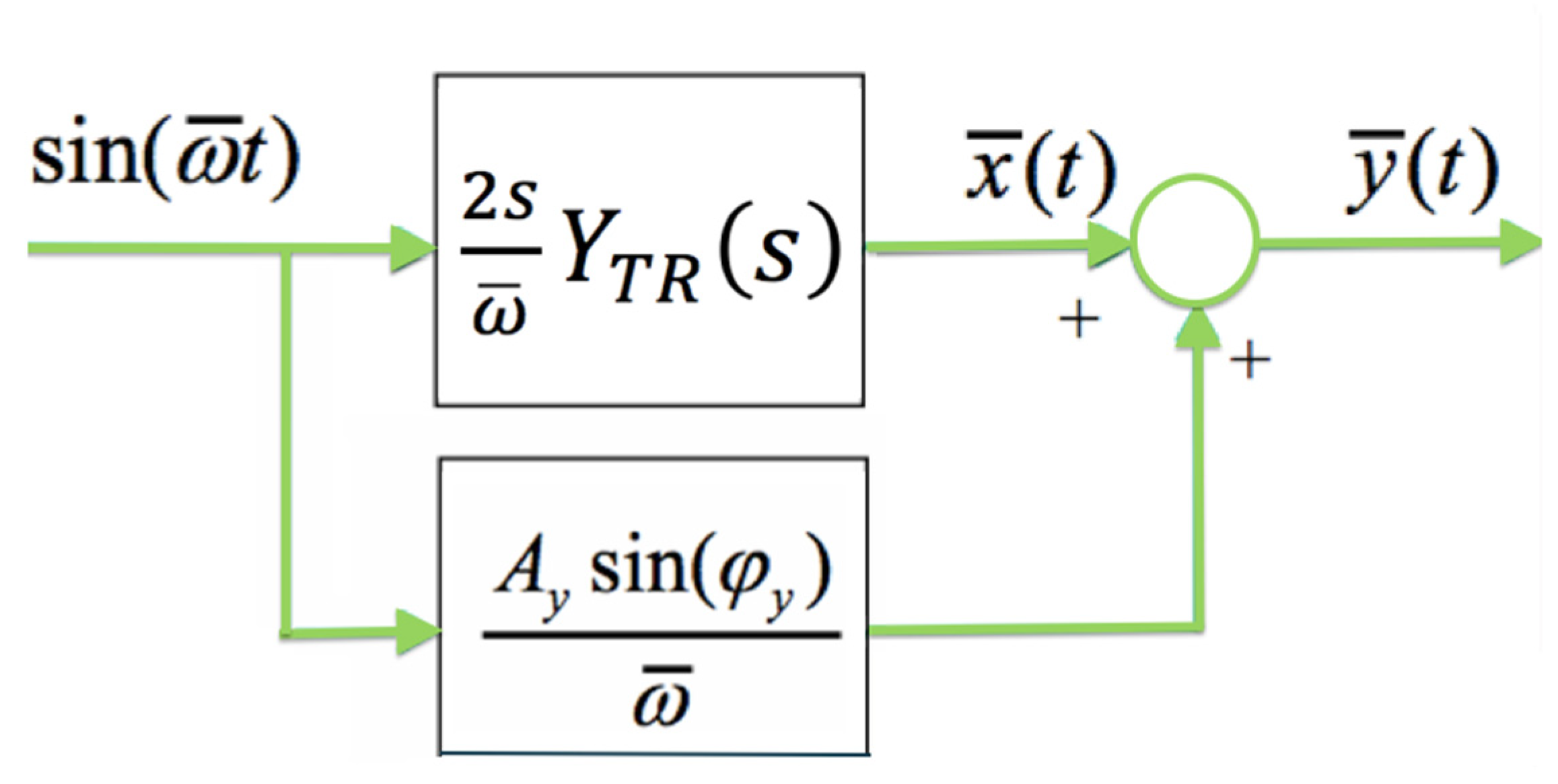
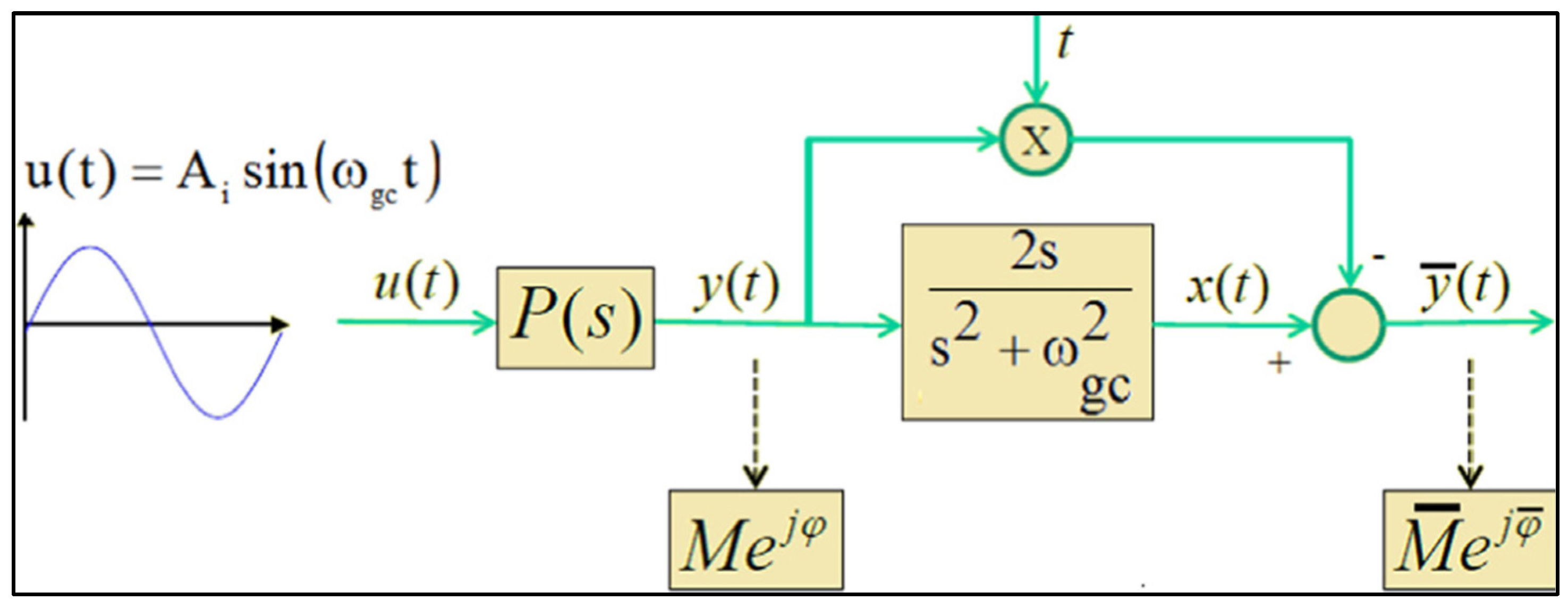
  • Perform a sine-test on the system using as the input signal a sine of the form u ( t ) = A u sin ω ¯ t . The sampling period for data acquisition is Ts, and the total number of measured samples is N.
  • Analyse the steady-state oscillation of y(t) to determine the amplitude Ay and phase φ y using (42)
  • Calculate the transient part yTR(t) as: y T R ( t ) = y ( t ) y s s ( t ) , with y s s ( t ) = A y sin ω ¯ t + φ y
  • Calculate the complex number A y ¯ e j φ y ¯ = 2 j T s k = 0 N 1 y T R k T s e j ω ¯ k T s + A y sin φ y ω ¯ .
  • Calculate the frequency response of the process and the frequency response slope at the frequency ω ¯ as: P j ω ¯ = M e j φ = A y A u e j φ y and d P ( j ω ) d ( j ω ) ω = ω ¯ = j A y ¯ A u e j φ y ¯ .

References

  1. Casas-Arroyave, F.D.; Fernández, J.M.; Zuleta-Tobón, J.J. Evaluation of a closed-loop intravenous total anesthesia delivery system with BIS monitoring compared to an open-loop target-controlled infusion (TCI) system: Randomized controlled clinical trial. Colomb. J. Anesthesiol. 2019, 47, 84–91. [Google Scholar] [CrossRef]
  2. Neckebroek, M.; Ionescu, C.M.; van Amsterdam, K.; De Smet, T.; De Baets, P.; Decruyenaere, J.; De Keyser, R.; Struys, M.M.R.F. A comparison of propofol-to-BIS post-operative intensive care sedation by means of target controlled infusion, Bayesian-based and predictive control methods: An observational, open-label pilot study. J. Clin. Monit. Comput. 2018, 33, 675–686. [Google Scholar] [CrossRef]
  3. Brogi, E.; Cyr, S.; Kazan, R.; Giunta, F.; Hemmerling, T.M. Clinical performance and Safety of Closed-Loop Systems: A systematic review and meta-analysis of randomized controlled trials. Anesth. Analg. 2017, 124, 446–455. [Google Scholar] [CrossRef]
  4. Carter, S.G.; Eckert, D.J. Effects of hypnotics on obstructive sleep apnea endotypes and severity: Novel insights into pathophysiology and treatment. Sleep Med. Rev. 2021, 58, 101492. [Google Scholar] [CrossRef] [PubMed]
  5. Garg, N.; Kalra, Y.; Panwar, S.; Arora, M.K.; Dhingra, U. Comparison of target concentration of propofol during three phases of live donor liver transplant surgery using a target-controlled infusion of propofol total intravenous anaesthesia—A prospective, observational pilot study. Indian J. Anaesth. 2024, 68, 971–977. [Google Scholar] [PubMed]
  6. Fahlenkamp, A.V.; Peters, D.; Biener, I.; Billoet, C.; Apfel, C.; Rossaint, R.; Coburn, M. Evaluation of bispectral index and auditory evoked potentials for hypnotic depth monitoring during balanced xenon anaesthesia compared with sevoflurane. Br. J. Anaesth. 2010, 105, 334–341. [Google Scholar] [CrossRef] [PubMed]
  7. Schiavo, M.; Padula, F.; Latronico, N.; Paltenghi, M.; Visioli, A. Individualized PID tuning for maintenance of general anesthesia with propofol and remifentanil coadministration. J. Process Control 2021, 109, 74–82. [Google Scholar] [CrossRef]
  8. Soltesz, K.; Van Heusden, K.; Dumont, G.A. In Automated Drug Delivery in Anesthesia; Models for control of intravenous anesthesia. Academic Press: Cambridge, MA, USA, 2020; pp. 119–166. [Google Scholar] [CrossRef]
  9. West, N.; van Heusden, K.; Görges, M.; Brodie, S.; Rollinson, A.; Petersen, C.L.; Dumont, G.A.; Ansermino, J.M.; Merchant, R.N. Design and evaluation of a Closed-Loop anesthesia system with robust control and safety system. Anesth. Analg. 2018, 127, 883–894. [Google Scholar] [CrossRef]
  10. Shah, P.; Agashe, S. Review of fractional PID controller. Mechatronics 2016, 38, 29–41. [Google Scholar] [CrossRef]
  11. Hegedus, E.T.; Birs, I.R.; Ghita, M.; Muresan, C.I. Fractional-Order Control Strategy for Anesthesia–Hemodynamic stabilization in patients undergoing surgical procedures. Fractal Fract. 2022, 6, 614. [Google Scholar] [CrossRef]
  12. Méndez, J.A.; Marrero, A.; Reboso, J.A.; León, A. Adaptive fuzzy predictive controller for anesthesia delivery. Control Eng. Pract. 2015, 46, 1–9. [Google Scholar] [CrossRef]
  13. Schiavo, M.; Padula, F.; Latronico, N.; Paltenghi, M.; Visioli, A. Experimental results of an event-based PID control system for propofol and remifentanil coadministration. Control Eng. Pract. 2023, 131, 105384. [Google Scholar] [CrossRef]
  14. Popescu, T.; Badau, N.; Mihai, M.; Hegedus, E.; Birs, I.; Copot, D.; Dulf, E.H.; Muresan, C.I. Advancing Anesthesia Education: Training on Modeling and Control for Enhanced Patient Care. In Proceedings of the 4th Workshop on Internet Based Control Education (IBCE), Ghent, Belgium, 18–20 September 2024. [Google Scholar]
  15. Parvinian, B.; Pathmanathan, P.; Daluwatte, C.; Yaghouby, F.; Gray, R.A.; Weininger, S.; Morrison, T.M.; Scully, C.G. Credibility evidence for computational patient models used in the development of physiological Closed-Loop controlled devices for critical care medicine. Front. Physiol. 2019, 10, 220. [Google Scholar] [CrossRef]
  16. Eleveld, D.J.; Colin, P.; Absalom, A.R.; Struys, M.M.R.F. Pharmacokinetic–pharmacodynamic model for propofol for broad application in anaesthesia and sedation. Br. J. Anaesth. 2018, 120, 942–959. [Google Scholar] [CrossRef] [PubMed]
  17. Van Den Berg, J.P.; Vereecke, H.E.M.; Proost, J.H.; Eleveld, D.J.; Wietasch, J.K.G.; Absalom, A.R.; Struys, M.M.R.F. Pharmacokinetic and pharmacodynamic interactions in anaesthesia. A review of current knowledge and how it can be used to optimize anaesthetic drug administration. Br. J. Anaesth. 2017, 118, 44–57. [Google Scholar] [CrossRef]
  18. Linassi, F.; Zanatta, P.; Spano, L.; Burelli, P.; Farnia, A.; Carron, M. Schnider and Eleveld Models for Propofol Target-Controlled Infusion Anesthesia: A Clinical comparison. Life 2023, 13, 2065. [Google Scholar] [CrossRef]
  19. De Keyser, R.; Muresan, C.I.; Ionescu, C.M. A novel auto-tuning method for fractional order PI/PD controllers. ISA Trans. 2016, 62, 268–275. [Google Scholar] [CrossRef]
  20. Caiado, D.V.; Lemos, J.M.; Costa, B.A.; Paz, L.A.; Mendonca, T.F. A polynomial design approach to robust control of neuromuscular blockade of patients subject to general anesthesia. In Proceedings of the 52nd IEEE Conference on Decision and Control, Firenze, Italy, 10–13 December 2013. [Google Scholar] [CrossRef]
  21. Monje, C.A.; Chen, Y.; Vinagre, B.M.; Xue, D.; Feliu, V. Fractional-Order Systems and Controls; Springer: Berlin/Heidelberg, Germany, 2010. [Google Scholar] [CrossRef]
  22. Lemos, J.; Caiado, D.V.; Costa, B.A.; Paz, L.A.; Mendonca, T.F.; Rabico, R.; Esteves, S.; Seabra, M. Robust control of Maintenance-Phase Anesthesia [Applications of control]. IEEE Control Syst. 2014, 34, 24–38. [Google Scholar] [CrossRef]
  23. Pawłowski, A.; Schiavo, M.; Latronico, N.; Paltenghi, M.; Visioli, A. Event-based MPC for propofol administration in anesthesia. Comput. Methods Programs Biomed. 2023, 229, 107289. [Google Scholar] [CrossRef]
  24. Ghita, M.; Ghita, M.; Copot, D. In Automated Drug Delivery in Anesthesia; An overview of computer-guided total intravenous anesthesia and monitoring devices—Drug infusion control strategies and analgesia assessment in clinical use and research. Academic Press: Cambridge, MA, USA, 2020; pp. 7–50. [Google Scholar] [CrossRef]
  25. Bataille, A.; Guirimand, A.; Szekely, B.; Michel-Cherqui, M.; Dumans, V.; Liu, N.; Chazot, T.; Fischler, M.; Le Guen, M. Does a hypnosis session reduce the required propofol dose during closed-loop anaesthesia induction? Eur. J. Anaesthesiol. 2018, 35, 675–681. [Google Scholar] [CrossRef]
  26. Schnider, T.W.; Minto, C.F.; Gambus, P.L.; Andresen, C.; Goodale, D.B.; Shafer, S.L.; Youngs, E.J. The influence of method of administration and covariates on the pharmacokinetics of propofol in adult volunteers. Anesthesiology 1998, 88, 1170–1182. [Google Scholar] [CrossRef] [PubMed]
  27. Mihai, M.; Birs, I.; Erwin, H.; Copot, D.; Neckebroek, M.; De Keyser, R.; Ionescu, C.M.; Muresan, C.I. First-Hand Design of a Fractional order PID for Controlling the Depth of Hypnosis during Induction. IFAC-Pap. 2024, 58, 186–191. [Google Scholar] [CrossRef]
  28. Åström, K.J.; Hägglund, T. Revisiting the Ziegler–Nichols step response method for PID control. J. Process Control 2004, 14, 635–650. [Google Scholar] [CrossRef]
  29. Ghita, M.; Neckebroek, M.; Muresan, C.; Copot, D. Closed-Loop Control of Anesthesia: Survey on actual trends, challenges and perspectives. IEEE Access 2020, 8, 206264–206279. [Google Scholar] [CrossRef]
  30. Padula, F.; Ionescu, C.; Latronico, N.; Paltenghi, M.; Visioli, A.; Vivacqua, G. Optimized PID control of depth of hypnosis in anesthesia. Comput. Methods Programs Biomed. 2017, 144, 21–35. [Google Scholar] [CrossRef] [PubMed]
  31. Merigo, L.; Padula, F.; Latronico, N.; Paltenghi, M.; Visioli, A. Optimized PID control of propofol and remifentanil coadministration for general anesthesia. Commun. Nonlinear Sci. Numer. Simul. 2018, 72, 194–212. [Google Scholar] [CrossRef]
  32. Dumont, G.A.; Martinez, A.; Ansermino, J.M. Robust control of depth of anesthesia. Int. J. Adapt. Control Signal Process. 2008, 23, 435–454. [Google Scholar] [CrossRef]
  33. Thomas, E.; Martin, F.; Pollard, B. Delayed recovery of consciousness after general anaesthesia. BJA Educ. 2020, 20, 173–179. [Google Scholar] [CrossRef]
  34. Paolino, N.; Schiavo, M.; Latronico, N.; Padula, F.; Paltenghi, M.; Visioli, A. On the Use of FOPID Controllers for Maintenance Phase of General Anesthesia. Appl. Sci. 2023, 13, 7381. [Google Scholar] [CrossRef]
  35. De Keyser, R.; Muresan, C.I.; Ionescu, C.M. Autotuning of a robust fractional order PID controller. IFAC-Pap. 2018, 51, 466–471. [Google Scholar] [CrossRef]
  36. Copot, C.; Muresan, C.; Ionescu, C.-M.; Vanlanduit, S.; De Keyser, R. Calibration of UR10 Robot Controller through Simple Auto-Tuning Approach. Robotics 2018, 7, 35. [Google Scholar] [CrossRef]
  37. De Keyser, R.; Ionescu, C.M.; Festila, C. A one-step procedure for frequency response estimation based on a Switch-Mode transfer function analyzer. In Proceedings of the 50th IEEE Conference on Decision and Control and European Control Conference, Orlando, FL, USA, 12–15 December 2011. [Google Scholar] [CrossRef]
Figure 1. Proposed setup for the sine test.
Fractalfract 09 00317 g001
Figure 2. Closed-loop control of induction phase using PID.
Fractalfract 09 00317 g002
Figure 3. Sine test simulation for one patient.
Fractalfract 09 00317 g003
Figure 4. FO-PI disturbance rejection test for the nominal case.
Fractalfract 09 00317 g004
Figure 5. The control signal of the FO-PI controller for the nominal case.
Fractalfract 09 00317 g005
Figure 6. FO-PID disturbance rejection test for the nominal case.
Fractalfract 09 00317 g006
Figure 7. FO-PI disturbance rejection test for another patient.
Fractalfract 09 00317 g007
Figure 8. Personalised FO-PI controllers closed-loop simulations.
Fractalfract 09 00317 g008
Figure 9. Personalised FO-PID controllers closed-loop simulations.
Fractalfract 09 00317 g009
Table 1. Personalised FO-PI/PID simulations.
PatientTTs for
FO-PI (Seconds)
TTs for
FO-PID (Seconds)
IAEBIS in Safe
Range of 40–60?
Positive
Dist.
Negative Dist.Positive
Dist.
Negative Dist.FO-PIFO-PID
1677410913421382508Yes
29412413220730023507Yes
3627410212719772251Yes
4768611514723042658Yes
5637510212619872205Yes
6738811315622852775Yes
7768511414022382473Yes
Disclaimer/Publisher’s Note: The statements, opinions and data contained in all publications are solely those of the individual author(s) and contributor(s) and not of MDPI and/or the editor(s). MDPI and/or the editor(s) disclaim responsibility for any injury to people or property resulting from any ideas, methods, instructions or products referred to in the content.

