Experimental Study of Confining Pressure-Induced Fracture Network for Shale Gas Reservoir Under Triaxial Compression Conditions

Abstract

The experimental study of shale fracture development is very important. As a channel of permeability, a fracture has a great influence on the development of shale gas. This study presents the results of a fracture evaluation in the Silurian Longmaxi Shale using the laboratory triaxial compression experiments and CT reconstruction, considering both mechanical properties and fracture network multi-dimensional quantitative characterization. The results indicate that the plastic deformation stage of shale lasts longer under high confining pressure, whereas radial deformation is restricted. Confining pressure has a nice linear connection with both compressive strength and elastic modulus. The 2D fractal dimension of radial and vertical cracks is 1.09–1.28 when the confining pressure is between 5 and 25 MPa. The 3D fractal dimension of the fracture is 2.08–2.16. There is a linear negative correlation at high confining pressure (R² > 0.80) and a weak linear association between the 3D fractal dimension of the fracture and confining pressure at low confining pressure. The fracture angle calculated by the volume weight of multiple main cracks has a linear relationship with the confining pressure (R² > 0.89), and its value is 73.90°–52.76°. The fracture rupture rate and fracture complexity coefficient are linearly negatively correlated with confining pressure (R² > 0.82). The Euler number can well characterize the connectivity of shale fractures, and the two show a strong linear positive correlation (R² = 0.98). We suggest that the bedding plane gap compression, radial deformation limitation, and interlayer effect weakening are efficient mechanisms for the formation of shale fracture networks induced by confining pressure, and that confining pressure plays a significant role in limiting and weakening the development of shale fractures, based on the quantitative characterization results of fractures.

1. Introduction

Exploration and development of unconventional resources, such as shale gas, have attracted public attention in recent years as a means of addressing the environmental crisis. The effective exploitation of shale gas mainly depends on hydraulic fracturing [1,2,3]. The complex in-situ stress conditions and highly diverse mechanical characteristics of shale add to the complexity of the mining operations [2]. Furthermore, the distinct bedding structure of shale gives all its characteristics a high degree of heterogeneity, which results in hydraulic fracturing producing numerous fractures in its internal morphological diversity. The effective development of shale gas has been significantly impacted by the significant variations in fracture morphology and connectivity under various compression circumstances, as demonstrated by several domestic and international studies. Therefore, the safe and effective development of shale gas resources greatly requires an in-depth examination of fracture propagation properties in shale, including geometric morphology and spatial distribution [1,3].

These are the primary areas of difficulty for the investigation of shale fracture propagation: Shale can produce numerous fractures and has strong brittleness properties. The mechanical characteristics of shale exhibit significant variation due to its distinct bedding structure. Furthermore, the weakening structure of the bedding plane is intimately linked to the fracture network created by the load. These factors make it challenging to characterize shale fractures, particularly in terms of quantitative characterization [4,5,6,7,8]. Most of the current research on characterizing shale fractures focuses on quantitative characterization with imprecise parameters and visual qualitative characterization. Wang et al. [9] used nano-transmission X-ray microscopy combined with 3D model to analyze the morphology of shale pores and micro-fractures. Gou et al. [10] used a CT scan. CO₂ and N₂ adsorption are used to qualitatively identify the pores and fractures of the Longmaxi Formation shale and quantitatively characterize the fracture trend and connectivity. Qi et al. [11] used CT three-dimensional reconstruction technology to characterize the location and morphology of a single fracture in shale and calculated its 3D fractal dimension. Based on CT three-dimensional reconstruction, Wang et al. [12] further combined fractal dimension with complexity coefficient to qualitatively and quantitatively characterize the spatial distribution characteristics of fractures after shale fracturing.

The research demonstrates that the use of CT imaging technology allows for the visual characterization of rock fracture expansion, which is essential for the quantitative assessment of rock fracture networks [13,14,15,16]. However, the existing correlation studies lack a suitable parameter for the characterization of shale fracture connectivity. In addition, the complexity of shale fractures has not been precisely described in several dimensions, and the parameters employed in the current quantitative characterization of shale fractures are insufficiently thorough. Furthermore, the coupling relationship between the complexity of shale fractures and their fractal characteristics cannot be clearly identified, and the correlation between the parameters in the quantitative characterization of shale fractures in the current study and the cross-scale characterization of multiple parameters has not been fully demonstrated.

To simulate the underground stress conditions of shale in the middle and deep layers (1000~2000 m), we used the constant speed loading method (0.3 mm/min) to apply different confining pressures (5, 10, 15, 20, and 25 MPa) to the shale. CT technology is utilized to achieve the accurate extraction of shale fractures following 2D and 3D investigations to quantitatively characterize the fracture propagation under triaxial stress. Herein, we use the relevant parameters of quantitative characterization of coal samples to characterize shale fractures and investigate the applicability of parameters and the distribution characteristics of fractures under shale mechanical conditions. The following questions are intended to be discussed in this contribution: (1) What variations exist in the distribution patterns of shale fracture under different confining pressures (5, 10, 15, 20, and 25 MPa)? (2) Are the quantitative characterization parameters, like fracture rate and connectivity, adequate for shale? (3) What mechanism underlies the variation in shale fracture distribution and morphology brought on by confining pressure?

2. Materials and Methods

The shale samples were taken from the outcrop shale of the Silurian Longmaxi Formation in the southern Sichuan Basin. The predominant compositions in these siliceous shale samples, identified by XRD analysis, included quartz (22.3%), calcite (32.5%), clay (1.5%), and dolomite (43.7%). According to the indoor mechanical test, due to the strict standards for the uniformity and integrity of shale samples, complete and unfractured shale blocks were selected for sampling. All samples have a borehole perpendicular to the laminated plane, as shown in Figure 1. Three parallel experimental groups (A, B, and C) were established to prevent unintentional mistakes and restore the true formation stress conditions (middle and deep shale) because mechanical tests are heavily influenced by human behavior. Five samples in each group were subjected to confining pressure settings of 5 MPa, 10 MPa, 15 MPa, 20 MPa, and 25 MPa.

Compression tests were performed using the TAW-2000 high-temperature and high-pressure triaxial experimental machine (Figure 1) developed by Chaoyang Test Instrument Co., Ltd. (Changchun, China). The study tested the compressive failure characteristics of laminated shale at five confining pressure levels at a loading rate of 0.03 mm/min, respectively. The stress–strain curves of samples under various experimental settings and the fractures in damaged samples were analyzed to study the geomechanical properties of laminated shale. The CT scanning experiments were all completed by the X-ray detection equipment GE Phoenix V|tome|X S240 CT by Youer Hongxin Testing Technology (Shenzhen) Co., Ltd. (Shenzhen, China). (Figure 2) [14]. The specific parameters of this equipment are as follows: maximum tube voltage, power: 240 KV, 320 W; minimum voxel: 1 micron; ensemble magnification: 1.46–100×, nanometer; the focus ray tube can reach 200×; detail resolution: up to <1 micron; maximum sample weight: 10 kg. The equipment is capable of rapid data collection and 3D reconstruction, in addition to robust data analysis, 2D and 3D detection, and detection of samples. The accuracy of the equipment is enough to observe the expansion and development of fractures inside the shale. The workflow is shown in Figure 2.

3. Results and Discussion

3.1. Effect of Confining Pressure on Stress–Strain Relations

The stress–strain curves of the samples for β of 0° under a confining pressure of 5, 10, 15, 20, and 25 MPa are presented in Figure 3. Combined with the analysis of previous related results [17,18], three stages could be identified in the stress–strain curves of the samples: the initial stage corresponds to elastic deformation, the second stage to plastic deformation, and the third stage to residual stress.

Meanwhile, it is worth noting that the shale samples with a confining pressure of 25 MPa always show the highest stress–strain slope and peak strength. However, the radial deformation of every sample is nearly the least when the confining pressure is 25 MPa. This suggests that the mechanical behavior of shale samples is significantly limited by high confining pressure. This result has also been confirmed in previous studies [17,19]. Chen et al. [19] conducted triaxial stress tests on black shale samples with various lamination angles to study the mechanical properties of black shale. The complete stress–strain curves and failure modes of black shale samples were obtained, and the effects of confining pressure and lamination angle on the mechanical behavior and failure modes of black shale were compared and analyzed. Their investigation into how confining pressure affected shale’s compressive strength reveals that there was a positive linear correlation between the compressive strength of shale and the rise in confining pressure. The compressive strength of the results obtained by Chen et al. is higher than that of this study (Figure 4). However, both sets of data demonstrate a strong linear positive association between confining pressure and compressive strength. This shows that the increase in confining pressure inhibits the damage to shale, and the compressive strength increases gradually.

3.2. Strength and Deformation Characteristics

The influences of confining pressure on the deformation characteristics of the shale samples are shown in Figure 5. The compressive strength and elastic modulus of shale samples increase linearly with increasing confining pressure. The high confining pressure shale samples are distributed in a split state, and the number of fractures is about 2–3, indicating that high confining pressure limits the radial deformation of shale and inhibits the overall development of fractures. However, Poisson’s ratio exhibits a complex nonlinear shift that lacks clear regularity as confining pressure increases (Figure 5c).

Figure 6 shows the failure features of laminated shale, and the failure features vary significantly with confining pressure. The failure characteristics are depicted in Figure 6b, where it is evident how these characteristics change dramatically with confining pressure. The shale sample is loaded to generate many intersecting fractures under low confining pressure (σ₃ < 15 MPa), while the distribution condition is complicated. Radial fractures have formed along the layer on the sample surface when the confining pressure is between 5 MPa and 15 MPa. In addition, the sample produced radial fractures along the loading direction, which are staggered with axial fractures and accompanied by many small fractures. The sample did not fail preferentially on the lamination plane due to the high confining pressure (σ₃ > 15 MPa), which significantly restricts the radial failure of the sample along the inner layer and prevents further tensile failure. The shale sample subjected to high confining pressure exhibits a splitting state distribution with approximately only 2–3 fractures, indicating that the formation of fractures is limited under high confining pressure.

3.3. Reconstruction of Shale Fracture Models

Typical shale samples under each confining pressure (σ₃ = 5, 10, 15, 20, and 25 MPa) setting were chosen for a CT scanning test following the triaxial stress test. Avizo software (Version 2023.2) can accurately extract and identify fractures in CT data according to modules such as ‘Interactive Thresholding’, ‘Compute Ambient Occlusion’, and ‘Membrane Enhancement Filter’. The 3D visualization of fractures is realized by the ‘Volume Rendering’ module, as shown in Figure 7. The fracture morphologies can be extracted and demonstrated to reveal the fracture evolution characteristics in shale at different confining pressures.

3.4. Quantitative Characterization of Fractures

3.4.1. 2D Fractal Dimension

The surface of the sample fractures is statistically characterized using the fractal theory [20,21] to better investigate the geometric morphology and distribution of fractures. The 2D fractal dimension is a strictly lower-than-2 number that is higher than 1. When typical geometric features (circles, broken lines, and straight lines) are used, the outcome is 1. Fractal dimension is a useful metric for measuring and comparing the degree of irregularity and fragmentation in 2D images at various magnifications. The curve’s ability to fill the space is another useful signal. The fractal dimension decreases with the increase in curve smoothness.

In this research, the box-counting fractal dimension method [22,23] was employed due to its relative ease of mathematical calculation and applicability for characterizing the spatial distribution of fractures. To determine the dimension of a fractal object or set F, an evenly spaced grid cover is placed on the fractal, and the number of boxes needed to minimally cover it is counted. The variation in the number of boxes as the grid becomes finer is used to compute the box-counting fractal dimension. The following formula can be used to get the box-counting fractal dimension:

$$D_1=-\underset{\delta \to 0}{\lim }{\displaystyle \frac{{logN}_{\delta }\left(F\right)}{log\delta }}$$

(1)

where D₁ is the box-counting fractal dimension, δ is the side length of covering boxes, F is the fractal set, and N_δ(F) is the number of boxes.

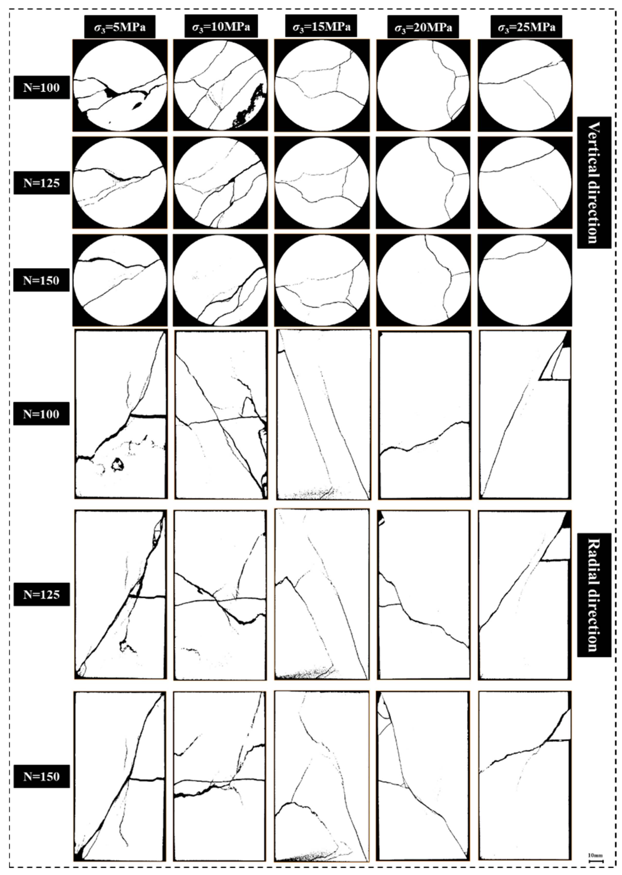
The axial load of the compression test is applied by raising the base of the apparatus, which will result in more severe damage along the top and bottom borders of the sample. The fracture distribution of the edge section is significantly inaccurate. Therefore, we selected the longitudinal and transverse slices of each sample numbered 100, 125, and 150 as the research object (these slices are closer to the central part of the sample) (Figure 8). When the confining pressure is low (σ₃ < 15 MPa), the radial binarized image mostly displays the cross distribution of shear and tensile fractures in the sample. Sample fractures typically occur in a single shear condition at high confining pressures (σ₃ > 15 MPa). The distribution of fractures gradually becomes single, while the number of fractures in both longitudinal and radial directions steadily decreases with an increase in confining pressure.

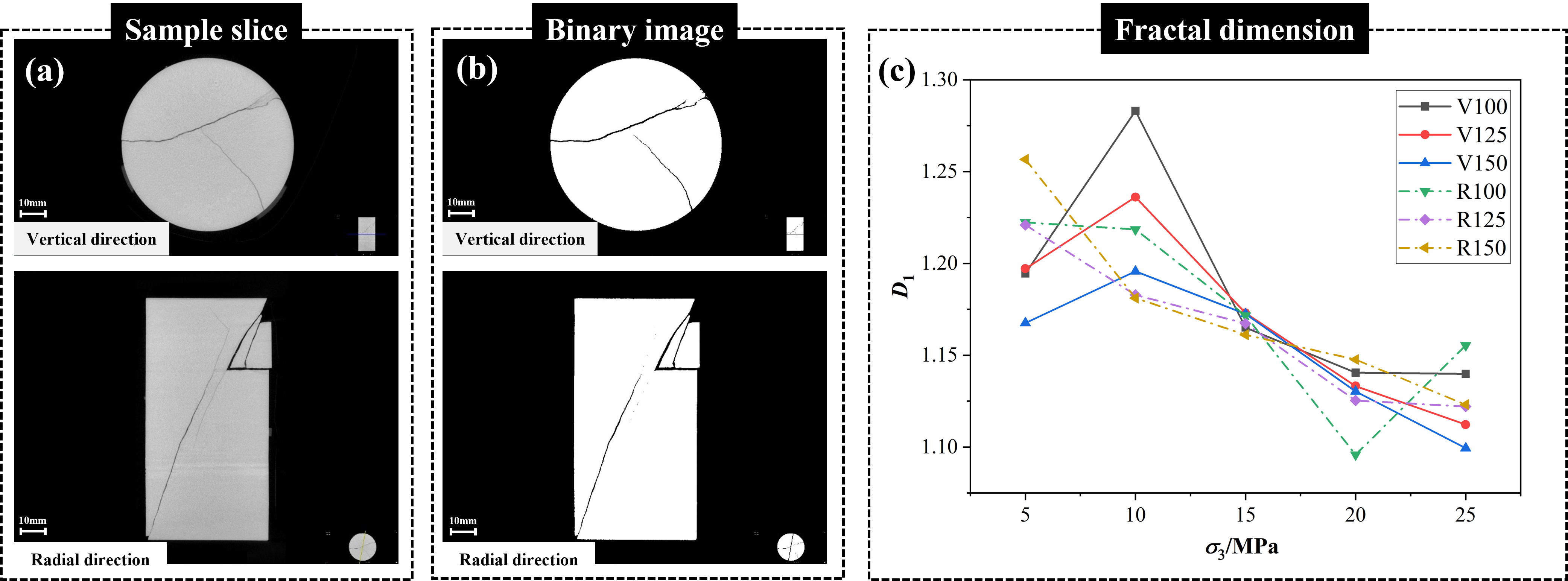
It is in line with the previously discussed sample failure mode. Concurrently, a linear decreasing trend is observed in the relationship between the confining pressure and the 2D fractal dimensions in both directions, as shown in Figure 9c. The physical definition of fractal dimension indicates that the form and distribution of fractures are more complicated the larger the fractal dimension. Therefore, it can be seen from the quantitative data that under low confining pressure, the distribution of axial slice fractures has no obvious law with the change in confining pressure. The complexity of radial slice fracture distribution decreases with the increase in confining pressure. The intricacy of the fracture distribution in both directions is inversely connected with the confining pressure at high confining pressures.

The average fractal dimensions of the three sets of slices in two directions are obtained to further evaluate the relationship between the confining pressure and the fractal dimension in the vertical and radial directions (Figure 10). The findings show that when confining pressure increases, the fractal dimension reduces linearly in both directions. The failure modes in the vertical and radial directions also show obvious regular changes with the increase in confining pressure. The failure mode of the slice in Figure 10 shows that the distribution pattern is more complex, the length is longer, and there are more fractures in both directions of the slice under low confining pressure. The interwoven occurrence of tensile and shear fractures characterizes the fracture morphology of radial slices under low confining pressure. The radial slice fracture morphology essentially shows a main shear fracture and a secondary fracture when the confining pressure is 20 MPa. When the confining pressure is 25 MPa, the fractures in both directions exhibit a single shear fracture, which is in line with the findings of the earlier research. The above analysis shows that the fractal dimension can accurately and quantitatively characterize the internal fracture changes of shale samples in two directions. In addition, the increase in confining pressure will not only affect its mechanical properties, but also greatly limit the expansion and development of radial fractures, resulting in the simplification of the whole fracture network.

3.4.2. 3D Fractal Dimension

The 3D visualization provides a more thorough observation of the geometric form and spatial distribution properties of fractures. The 3D fractal dimension of the 3D rebuilt fracture model is computed using the box dimension method [22,24,25] (Figure 11).

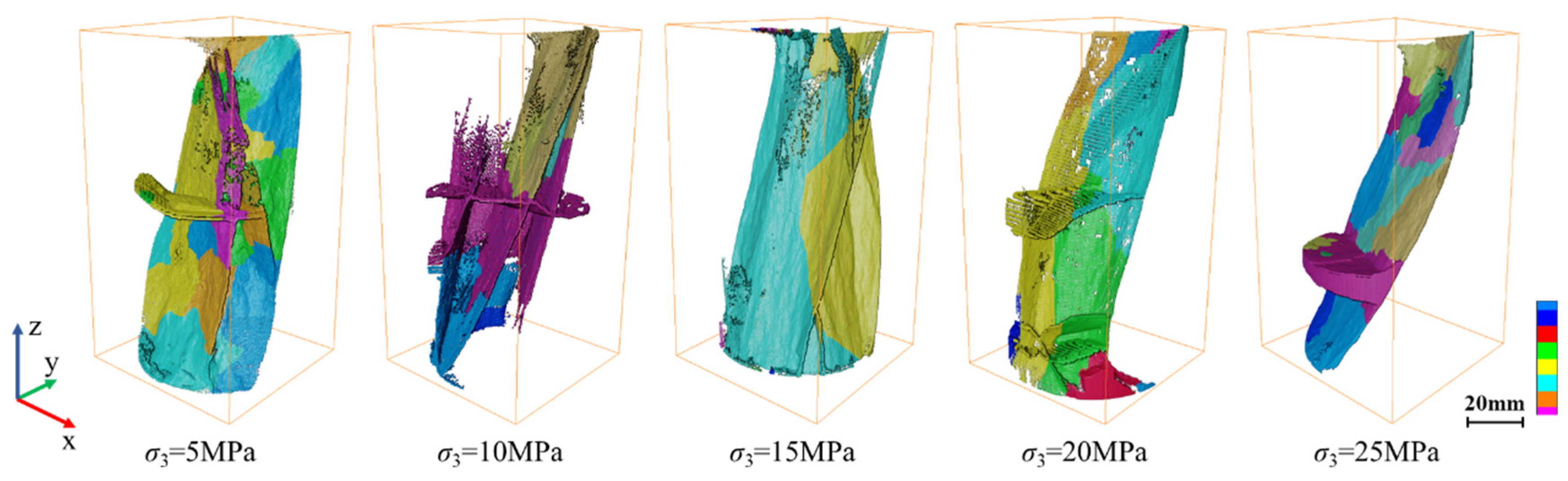
The quantity, shape, and spatial distribution properties of fractures are significantly influenced by the confining pressure, as indicated by the Avizo 3D reconstruction visual fracture model (Figure 11a). The sample has more than three main fractures that cross over when the confining pressure is 5–10 MPa. The main fractures are surrounded by a complicated fracture network made up of minor fractures. At a confining pressure of 15 MPa, the characteristics of the fracture distribution within the sample are obviously different. The main fractures are reduced to 2, with some minor fractures. Axial shear fractures are present in nearly all of them, while there is no significant radial fracture dispersion. The sample exhibits a single main fracture and several smaller fractures running parallel to the axial direction of the main fracture when the confining pressure reaches 20 MPa. The internal fractures of the sample show a flat main fracture accompanied by a small oblique fracture. When the confining pressure reaches 25 MPa, the geometric shape is single, and there is no minor fracture surrounding the main fracture at the same time.

According to the principle of the box-counting dimension method, a 3D reconstruction model of fractures is divided into many small cubes with a certain length δ_k. The small cubes cover all the fractures. The quantity N_δk of cubes corresponding to the length δ_k can be calculated. By changing the length δ_k of the cubes, we can obtain a series of the corresponding N_δk. Next, the fractal dimension can be calculated as follows:

$$D_2=\underset{n\to \infty }{\lim }{\displaystyle \frac{{lnN}_{{\delta }_k}\left(F_2\right)}{{-ln\delta }_k}}$$

(2)

where D₂ is the fractal dimension of the 3D fracture surface, F₂ is the cube covering the fracture, δ_k is the characteristic size of the small cube, and N_δk is the number of cubes with a length of δ_k.

The findings indicate that the fractal dimension and low confining pressure (σ₃ < 15 MPa) do not clearly correlate linearly. The fractal dimension rises to 2.158 when the confining pressure rises from 5 to 10 MPa. However, the fractal dimension exhibits a declining tendency under high confining pressure (σ₃ > 15 MPa). The regularity of the whole curve shows that as confining pressure increases, the fracture fractal size decreases, the fracture count decreases, and the distribution approaches a single shear shape. Both are highly correlated (R² > 0.8). The changing rule of the 2D fractal dimension is in line with this. Both can provide a quantitative explanation for why increasing confining pressure will significantly affect the formation and distribution of fractures in space.

Wang et al. [12] also used fractal theory and three-dimensional reconstruction technology to characterize the fracture development of shale under hydraulic fracturing. The findings demonstrated that increasing confining pressure prevented shale fractures from extending and prevented their volume transformation. Yang et al. [26] used triaxial compression and CT three-dimensional reconstruction techniques to investigate the fracture morphology and distribution features of tight sandstone. To further characterize fracture propagation, this research combined energy theory with fractal theory to propose energy dissipation and release laws. The findings demonstrated that high confining pressure significantly reduced the internal fractures of the sample, and the geometric shape was single. The fractal size of the fracture and the confining pressure both dropped linearly at the same time, but the amount of elastic strain energy that could be released increased. These findings are consistent with the results of this research, which show how confining pressure limits the growth of shale fractures from a fractal perspective.

3.4.3. Fracture Rate, Fracture Complexity Coefficient, and Fracture Connectivity

The fracture complexity coefficient and fracture rate are significant variables demonstrating how fractures form dynamically. It is possible to determine the sample’s fracture volume, overall volume, and 3D fractal dimension by using the Avizo software 3D reconstruction model of the CT picture. According to these data, we can calculate the fracture rate and the fracture complexity coefficient.

The ratio of the fracture volume to the shale sample’s total volume is known as the fracture rate [22]:

$$\phi ={\displaystyle \frac{V_f}{V_s}}$$

(3)

where V_f is the volume of fractures in a shale sample, and V_s is the total volume of a shale sample.

Based on the previous calculation of the fracture complexity coefficient of shale samples, the definition is as follows [27]:

$$F_c=D_2\times {\displaystyle \frac{\alpha }{90}}$$

(4)

where F_c is the fracture complexity coefficient, α is the fracture angle of the rock.

It can be seen from Equations (5) and (6) that the fracture angle of rock is an important parameter to determine the complexity coefficient of fracture. There is a significant inaccuracy in the old method, and only one of the primary fractures cannot adequately convey the intricacy of shale fractures. Therefore, each sample fracture is divided into many main cracks and numbered as (1, 2, 3, 4) (Figure 12), using Avizo’s “Extract subvolume” module. The rupture angle of each main crack is calculated, and then the weighted rupture angle of each crack is obtained according to the percentage of its crack volume to the total crack volume. The sum of the weight angles of ownership obtained for each sample is the new rupture angle [28]. The division is based on the size of the fracture volume (the fracture is less than 500 mm³) and the fracture angle difference (the fracture angle value between the main fractures is large).

$$F_c^{*}=D_2\times {\displaystyle \frac{{\alpha }^{*}}{90}}$$

(5)

$${\alpha }^{*}=\sum _{i=1}^3{\overline{\alpha }}_i\times {\displaystyle \frac{V_i}{V_f}}$$

(6)

where $V_i$ is the volume of each fracture, $V_f$ is the total volume of fractures, ${\overline{\alpha }}_i$ is the average value of the fracture angle of each fracture measured and divided, $F_c^{*}$ is a new fracture complexity coefficient, and α* is a new rupture angle. According to the calculation principle, the fracture angle calculation method works well when the rock develops several major fractures, the failure form is more complicated, while a single fracture is unable to compute the fracture angle.

The shale gas development heavily depends on the growth and creation of the internal fracture network. Since the permeability of shale is mostly determined by the connectivity of its fractures, the connectivity of shale fractures is a crucial quantity to describe its fractures. The connectedness of fractures in shale samples is quantitatively characterized by using the Euler number [29]. The Avizo Euler 3D module can determine the fracture Euler number. The object’s Euler–Poincaré number is calculated using this module. It serves as a gauge for a 3D complicated structure’s connectedness. The Euler number is a topologically invariant property of a three-dimensional structure, meaning that it is unaffected by elastic changes to the structure. It measures what might be called ‘redundant connectivity’—the degree to which parts of the object are multiply connected [30]. It is a measure of how many connections in a structure can be severed before the structure falls into two separate pieces (Figure 13).

$$E\mathrm{u}={\beta }_0-{\beta }_1+{\beta }_2$$

(7)

where, β₀ is the number of isolated fractures, β₁ is the number of connected fractures, and β₂ is the number of closed fractures.

According to the analysis results in

Table 1. The results of the fracture rate, complexity coefficient, and fracture connectivity.

Confining Pressure/MPa	Fracture Volume/mm3	Total Volume of Sample/mm3	Fracture Rate/%	Complexity Coefficient	Euler Number
5	5435.980	196,209.869	2.770	1.883	−391.750
10	4316.317	194,423.305	2.220	1.789	−321.730
15	4122.193	194,423.305	2.120	1.737	−205.454
20	4182.889	203,474.566	2.056	1.619	−30.824
25	3643.090	191,568.4827	1.902	1.225	88.800

, the fracture volume shows that the volume of fractures is practically steadily decreasing as the confining pressure increases. The biggest fracture volume occurs at 5 MPa confining pressure, while as the confining pressure rises above 15 MPa, the fracture volume sharply reduces. The fracture volume reduces by 33% when the confining pressure reaches 25 MPa compared to a confining pressure of 5 MPa. The increase in confining pressure clearly results in a decrease in fracture volume, which is particularly true considering the confining pressure is high. Table 1 displays the Euler number that was determined by Avizo. Based on the Euler number characterization, the fracture connectivity decreases with increasing Euler number. The study results show that there is a linear positive correlation between the confining pressure and the Euler number (Figure 14). A strong association exists between the two (R² > 0.9). Previous research [22,31] has shown that fracture connectivity improves with decreasing Euler number. As a result, it is evident that fracture connectivity deteriorates as confining pressure increases.

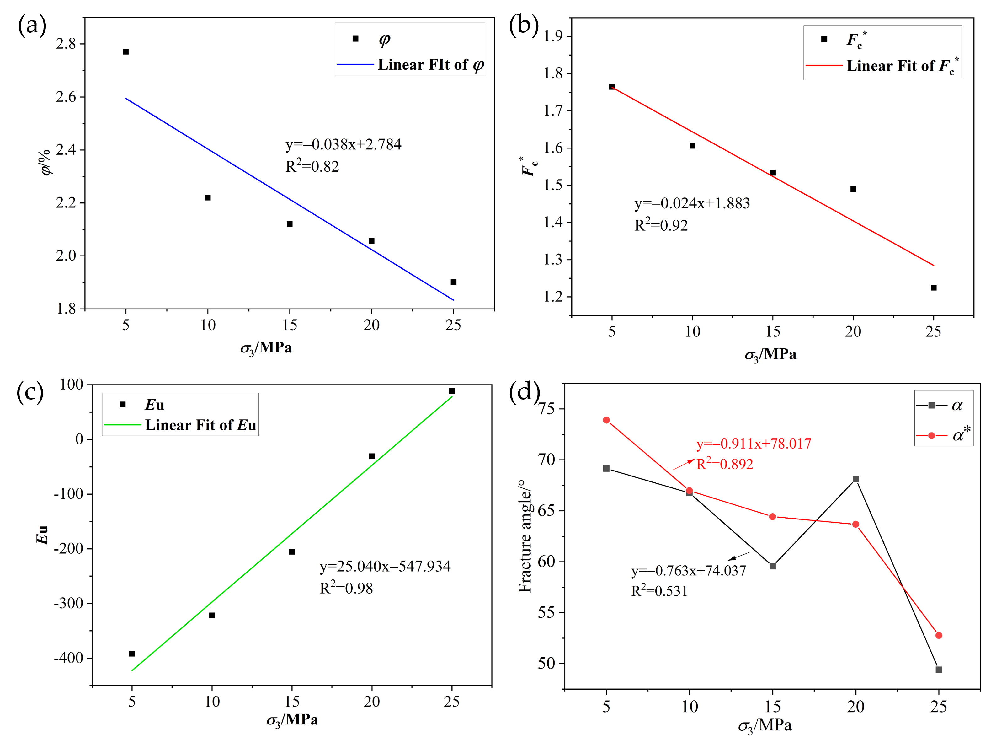
The changing trend of the sample fracture rate and the fracture complexity coefficient is almost the same, as shown in Figure 14. Confining pressure has a negative correlation with each of them. Furthermore, it shows a strong association (R² > 0.8) between the two and confining pressure. At confining pressures between 5 and 15 MPa, the visual complexity of the fracture model remains relatively unchanged. However, the fracture rate and complexity coefficient calculation results show that the two parameters of the fractures have significantly decreased in this range of confining pressure, indicating that the fracture development inside the sample is still quantitatively negatively correlated with the confining pressure. The fracture development is clearly less than that of the low confining pressure condition when the confining pressure exceeds 20 MPa, as demonstrated by both visualization and quantification. Meanwhile, three fracture modes, ranging in size from large to small, are present in the fracture complexity coefficient: tensile fracture is greater than shear fracture, which is consistent with earlier findings [32,33].

The radial expansion failure will occur along the lamination plane under the action of external load (β = 0°) due to the complex mineral arrangement and combination relationship and the significantly lower cementation degree of the lamination plane compared to the remainder of the area [19,34]. However, the existence of confining pressure provides a limiting force for the radial deformation of shale, and the greater the confining pressure is, the stronger the restriction is. The fracture distribution exhibits a single shear shape (almost no radial tensile failure) when the confining pressure is high enough. This occurs because the axial direction of the shale will experience macroscopic shear failure before the radial direction (deformation is limited).

In addition, we also verified the accuracy of and the differences between the two methods in calculating the fracture angle. The main fracture with the highest volume ratio is chosen as the benchmark for calculating the fracture angle in accordance with the conventional method. It is evident that there is a significant discrepancy between the results and the rupture angle determined using the weight calculation approach (Figure 14d). The fracture angle obtained by relying on the main fracture has poor regularity with the change trend of the confining pressure. The fracture angle determined by the greatest shale fracture exhibits an unusually high value at a confining pressure of 20 MPa. It is evident from the fitting correlation coefficient R² = 0.531 that there is little association between the confining pressure and the fracture angle determined using this method. However, there is a strong linear correlation between confining pressure and the fractal dimension and Euler number, which indicates that the fracture angle calculated by this method is not consistent with the results characterized by other parameters. With a confining pressure of 20 MPa, the division findings of the shale main fractures show that the fracture angles of the two main fractures are significantly different (Figure 12). The traditional calculation method uses the crack of serial number 1 as the basis for calculating the fracture angle, thus ignoring the influence of the main fracture of serial number 2 on the calculation of the fracture angle, resulting in a large error in the calculation of the fracture angle. It increases the difficulty of exploring the regularity between fracture angle and confining pressure. The correlation between the fracture angle calculated by the weight method and the confining pressure is good (R² = 0.892), which is consistent with the results characterized by other parameters. This demonstrates that the weight-based fracture angle calculation is more precise and dependable than the conventional approach, offering a useful computation technique for describing the fracture properties of shale.

3.4.4. Correlation Between Fracture Rate, Complexity Coefficient, Connectivity, and Fractal Dimension

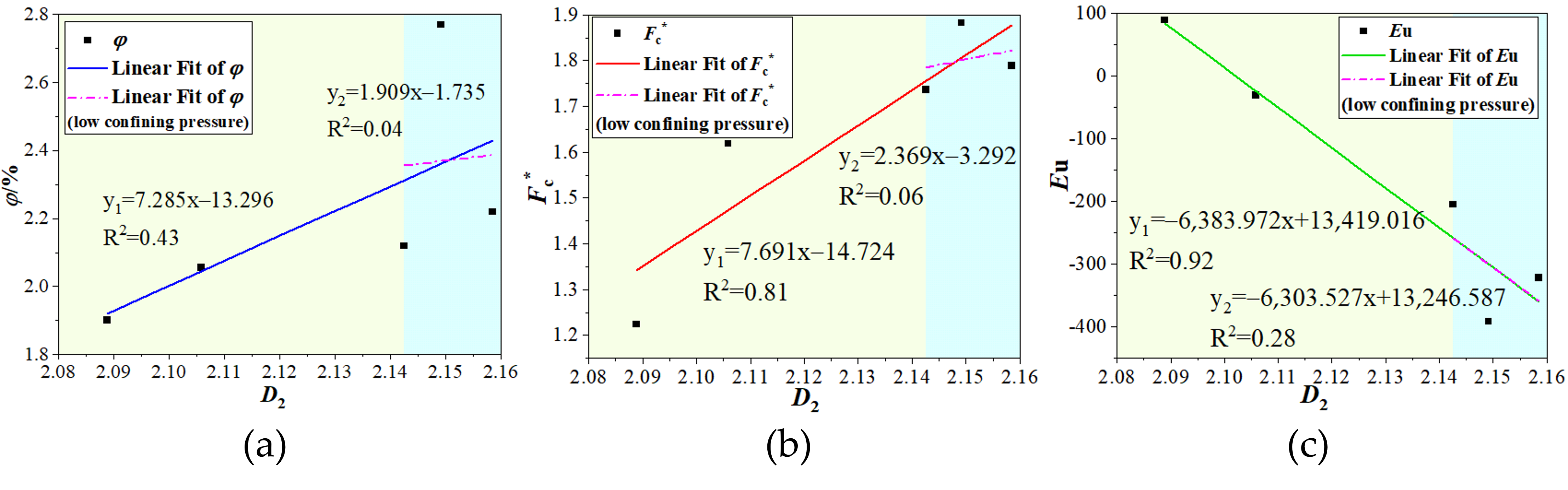
The fracture rate, fracture complexity coefficient, and fracture connectivity are correlated to the 3D fractal dimension of the fracture, as seen in Figure 15. It is evident that there is a definite linear positive connection between the fracture rate and 3D fractal dimension from R² = 0.435 (Figure 15a). 3D fractal dimension and the complexity coefficient have a significant (R² > 0.8) positive linear relationship (Figure 15b). The strongest link (R² > 0.9) is found between 3D fractal dimension and the Euler number, which is linearly negative (Figure 15c). The correlation coefficients R² between the three parameters and the 3D fractal dimension under low confining pressure are 0.04, 0.06, and 0.28. It shows that the correlation between the four is relatively weak under low confining pressure. Combined with the analysis of the distribution of fractures, the influence of low confining pressure on the morphology and distribution of fractures is not obvious. 3D fractal dimension, fracture rate, and complexity coefficient decrease, and the connectivity increases as the confining pressure increases. They all demonstrate that fracture formation and development are not facilitated by high confining pressure. This conclusion nearly agrees with Wang et al. [22]. Similar linear correlation rules were obtained by fitting coal sample data, such as fracture volume and fracture connectivity, with fractal dimension. The positive linear correlation between the parameters indicates that they are all suitable parameters for characterizing shale fractures, which provides a feasible theoretical calculation for the quantitative characterization of shale fracture networks.

3.4.5. Mechanism of Confining Pressure on Fractures

The ossification of fracture space can be realized by using the ‘Auto Skeleton’ module of Avizo. The centerline of filamentous structures is extracted from picture data using this module. The module can segment photos based on a user-defined threshold value, and it can also work with binary and gray value images. The module essentially completes a few separate compute modules that need to be run consecutively. The segmented image’s distance map is first computed (Figure 16a), and then the binary image is thinned until only a string of connected voxels is left (Figure 16b). The voxel skeleton is then converted to a Spatial Graph object (Figure 16c). The distance to the nearest boundary (boundary distance map) is stored at every point in the Spatial Graph object as a thickness attribute (Eval on Lines). The local thickness can be estimated using this value. The module accepts both out-of-core image data in the Large Disk Data format and normal image data (Uniform Scalar Field) as input. The outcome is thick information in the form of lines that are saved in the Spatial Graph format. Therefore, the fracture ossification diagram provides some crucial information.

Figure 16 shows that at low confining pressure, the Trace Lines density of the spatial transformation of fractures in the sample is substantially larger than at high confining pressure. The complexity of fracture space can be observed intuitively, and low confining pressure conditions are conducive to the development of fractures. In addition, the thickness of the trace increases with its color bias toward red. The sample is axially loaded, which means that the edges of both ends have an extensive amount of damage. Therefore, the analysis should avoid using areas with a lot of inaccuracy. The more connected the fracture space, the thicker the trace lines are, which is combined with the connectivity computation method. In addition, the density and thickness of Trace Lines are noticeably higher in places with radial tensile fractures inside the sample than in other regions. This indicates that the degree of damage in this region is higher when the shale experiences radial tensile failure, which promotes the development of a fracture network and an increase in fracture connectivity.

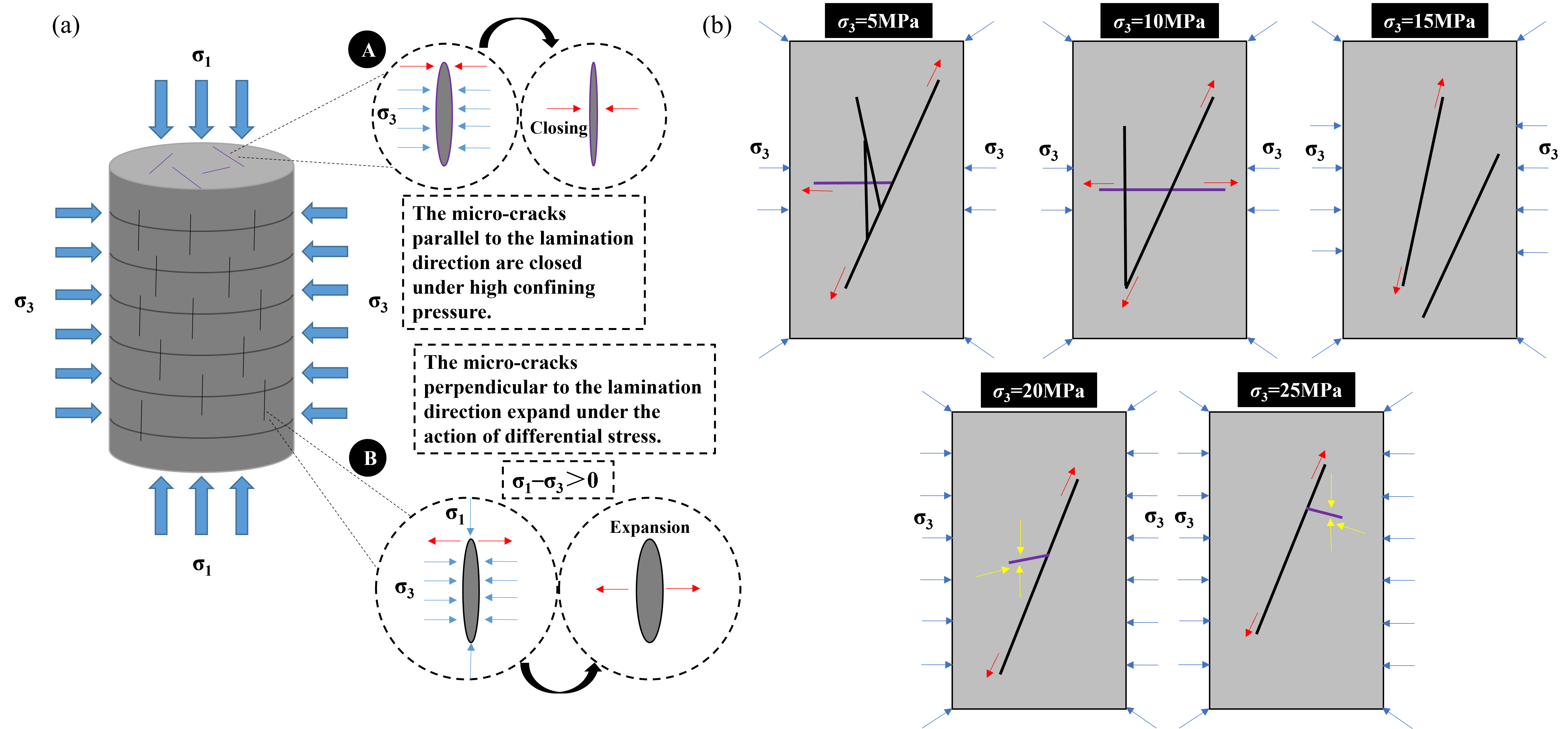
The micro-fractures and micro-pores between the bedding planes are compressed by the high confining pressure, which helps the bedding plane resist deformation. Sarout et al. [35] proposed that micro-fractures perpendicular and parallel to the lamination plane may already exist inside the shale sample during drilling (Figure 17a). According to the classical rock mechanics theory, the rock has a large compliance in the direction perpendicular to the bedding. The high confining pressure will close the micro-fractures in two directions. When σ₁−σ₃ > 0, the micro-fractures perpendicular to the lamination direction expand prior to the micro-fractures parallel to the lamination direction. The micro-fractures perpendicular to the lamination direction will continue to grow and intersect as the axial stress increases, eventually leading to macroscopic fracture.

Furthermore, the high confining pressure will provide a limiting force to the radial direction of the sample and hinder the radial deformation inside the sample, as shown in Figure 17b. Xie et al. [36] demonstrated that increasing confining pressure can effectively diminish the interlayer effect of composite structures, hence increasing the strength of rock mass with weak structural planes, by examining the failure behavior of layered rock under genuine triaxial stress. Yang et al. [37] explored the evolution of shale acoustic emission under conventional triaxial compression. The results show that under low confining pressure, the samples of β = 0° shale show tensile fracture failure along the lamination plane, and multiple tensile fractures appear along the lamination plane. The sample develops one or two shear fractures at high confining pressure, and the failure is dominated by the shear fractures. In this case, the main fractures will be formed by shear fractures that appear before tensile fractures [38]. The development of radial tensile fractures under high confining pressure is not clear because shear fractures preferentially damage the integrity of shale and penetrate several bedding planes. Shear fractures prevented radial tensile fractures from expanding along the bedding plane.

4. Conclusions

(1) The reconstructed 3D digital fracture model reflects the distribution and propagation characteristics of 3D fractures in shale. The radial and vertical portions of the shale fracture have a 2D fractal dimension of 1.09–1.28, which has a linearly negative correlation with the confining pressure. Shale fractures have a 3D fractal dimension of 2.08–2.16. The three-dimensional fractal dimension has a poor linear connection with low confining pressure (σ₃ ≤ 15 MPa). However, the 3D fractal dimension of fractures is linearly negatively correlated with a correlation coefficient R² > 0.8 under high confining pressure (σ₃ > 15 MPa).

(2) The fracture angle calculated according to multiple main fractures of shale is 73.90°–52.76°, which is linearly negatively correlated with confining pressure, and the correlation coefficient R² > 0.89. The fracture rate and fracture complexity coefficient are linearly negatively correlated with confining pressure, and the correlation coefficient R² > 0.82. The Euler number can well characterize the connectivity of shale fractures, and the two show a strong linear positive correlation (R² = 0.98). The 3D fractal dimension is well correlated with these quantitative factors. The accuracy of the parameters is good, and the correlation coefficient R² is 0.43, 0.81, and 0.92. Furthermore, the characterization results of several quantitative parameters demonstrate that the growth of shale cracks is significantly restricted and weakened by the confining pressure.

(3) Radial fractures will increase fracture connectivity. Furthermore, macroscopic fractures can arise from core drilling-induced micro-fractures, which are perpendicular to the lamination plane and preferentially enlarge under differential stress. The lamination plane gap can be easily compacted by high confining pressure, which also limits radial deformation and eliminates the interlayer effect. In addition, shear fractures dominate failure and hinder the propagation of radial tensile fractures. Therefore, we suggest that the lamination plane gap compression, radial deformation limitation, and weakening of the interlayer effect may be the effective mechanisms of the confining pressure-induced shale fracture network.

(4) The method of multi-dimensional quantitative parameter evaluation of shale fractures and the mechanism of confining pressure affecting its fractures proposed in the study can provide theoretical support and ideas for the effective transformation of hydraulic fracturing fractures in deep shale. In addition, the experimental conditions of the study are limited to confining pressure. The evaluation of shale fractures under the combination of high temperature and high pressure can be used to inform future research and provide practical theoretical direction for the development of deep shale.