1. Introduction
Let
A be a
matrix with real entries that is expansive, i.e., all the eigenvalues of
A have moduli
. Given an integer
, let
be a set of
N vectors. Define affine contracting functions on
as follows:
The family of functions
is called a self-affine iterated function system (IFS) [
1]. According to Hutchinson’s theorem [
2], there exists a unique, nonempty, compact set
that satisfies the following:
The compact set
K is canonically termed a self-affine set or an attractor of the IFS. When
holds and
K possesses a nonempty interior, the attractor is classified as a self-affine tile [
3], characterized by its capacity to tessellate the ambient space through translational copies. In a specialized case where the linear component
A constitutes a similitude satisfying
with
(scaling factor) and an orthonormal matrix
R, the system
is designated as a self-similar IFS, and its attractor
K accordingly becomes a self-similar set.
Both the IFS and its attractor are the main research objects of fractal geometry and dynamical systems. Let
be the symbolic space associated with the IFS, where
and
. Then, write the following:
If
, we assume
for the sake of simplicity. Then, we consider
with the following:
Next, write
. By iterating (
2), the self-affine set
K is of the following form for any
:
The symbolic space
naturally inherits a tree structure through standard word concatenation, where we denote the vertical edge set by
. This construction explicitly reveals
as an
N-ary tree. Such a combinatorial structure plays a crucial role in calculating the Hausdorff dimension of the associated attractor
K (see [
1,
2,
4]).
In the current field of fractal geometry, the open set condition is perhaps one of the most fundamental and useful separation conditions to track the iteration rules. The IFS
is said to satisfy the
open set condition (OSC) [
1,
2], if there is a nonempty, bounded, open set
such that
and
for all
. If the additional condition
holds, we say that the IFS satisfies the
strong open set condition (SOSC).
Self-similar IFSs with the OSC can be handled easily, and the Hausdorff dimension of self-similar sets can be calculated accurately. In particular, Schief [
4] proved a well-known result regarding the characterization of the OSC in self-similar IFSs. Recently, Fu, Gabardo, and Qiu [
5] extended Schief’s result and obtained a generalization on self-affine IFSs by replacing the Euclidean metric with a quasi-metric
introduced by He and Lau [
6]. Under the quasi-metric
(see details in
Section 2), the self-affine IFS (
1) exhibited a similarity structure as
where
. It allowed for better dimensional estimates of
K through the generalized Hausdorff measure
and the generalized Hausdorff dimension
(please refer to [
6] for definitions).
Theorem 1 ([
5,
6])
. Let the IFS be as in (1), then the following are equivalent: - (i)
the OSC holds;
- (ii)
the SOSC holds;
- (iii)
, where ;
- (iv)
for all and is uniformly discrete, i.e. there exists such that for any .
When the OSC fails for an IFS, iterations inevitably generate overlaps, and the resulting attractor
K exhibits intricate geometric complexity. To address this challenge, the
weak separation condition (WSC) introduced by Lau and Ngai [
7] (see also [
8]) serves as a pivotal tool for analyzing self-similar IFSs with overlaps. While weaker than the OSC, the WSC retains key analytical properties (e.g., controlled overlapping scales) and maintains the tractability of the iterative process.
Deng [
9] generalized the concept of WSC as follows: A self-affine IFS
satisfies the WSC if, for every bounded set
, there exists
such that
This condition effectively quantifies overlapping multiplicity while accommodating affine distortions. A systematic exposition of the OSC, WSC, and other separation conditions and their relationships was comprehensively presented in the survey paper [
10].
Theorem 2 ([
9])
. Let the IFS be as in (1), then the following are equivalent: - (i)
the WSC holds;
- (ii)
there exists such that for any , either or ;
- (iii)
for any given bounded subsets , there exists such that for all and ;
- (iv)
for any , there exists a constant such that for any integer and any bounded set with diameter ,
Motivated by the previous works, we propose a novel characterization of the OSC and WSC in a self-affine IFS through graph-theoretic invariants. Before presenting our main theorems, we need some notation on graphs.
For an
N-ary tree
, we define horizontal edges as follows:
where
, and
is a constant. Let
. Then, the graph
is an augmented tree (see Definition 2). The concept of augmented tree was initially introduced by Kaimanovich [
11] to study the Sierpinski graph. Later, Lau and Wang [
12] developed his idea into a large class of self-similar sets.
If the IFS in (
1) satisfies the OSC, by Theorem 1,
holds for any distinct
. If the IFS does not satisfy the OSC, it may occur that
for
. In this case, we may modify the augmented tree
by identifying
for
, and let
be the quotient space of the graph
. The detailed modification can be found in
Section 3.
A graph is of bounded degree if , where is the total number of edges joining x.
Theorem 3. Let the IFS be as in (1). Then, we have the following: - (i)
The OSC holds if and only if the graph G is of bounded degree.
- (ii)
The WSC holds if and only if the quotient space is of bounded degree.
The idea of the proof is based on graph theory and the iteration rule of an IFS under the quasi-metric . We provide an example (see Example 1) to illustrate the conclusion.
Recently, Gromov hyperbolicity andthe hyperbolic boundaries of augmented trees induced by self-similar IFSs have attracted considerable attention (see [
11,
12,
13,
14,
15,
16,
17]). However, there are very few related studies on self-affine IFSs. In the second part of this paper, we demonstrate that the augmented tree
G inherently possesses Gromov hyperbolicity. This enables the establishment of a canonical association between self-affine IFSs and Gromov hyperbolic graphs, notably achieved without imposing separation conditions.
Theorem 4. For any IFS as in (1), the augmented tree is always a Gromov hyperbolic graph (see Definition 1). Moreover, the hyperbolic boundary is Hölder equivalent to the self-affine set K, that is, there exists a homeomorphism such that the following can be obtained::where and is a visual metric on G. The paper is organized as follows:
Section 2 describes the basic definitions and properties of Gromov hyperbolic graphs and augmented trees induced by IFSs.
Section 3 is devoted to establishing Theorem 3 (by proving Theorems 5 and 6) and Theorem 4.
2. Augmented Tree Induced by IFS
Following the notation in graph theory, let be a connected graph, where X is a countably infinite set of vertices and stands for the set of edges. Let denote a geodesic path from x to y in X, i.e., a path connecting with the shortest length. Denote the distance between x and y as . The degree of a vertex x is defined by , the total number of edges connecting x. A graph is of a bounded degree if .
The bounded degree of a graph is an important tool for studying the random walks on graphs; however, it should be distinguished from another concept, “locally finite”. A graph is said to be locally finite if every vertex has finite degree (i.e., ).
Fix a vertex o in X as a root of the graph. Let denote the distance from the root o to the vertex x. means that x is located on the n-th level of the graph. A graph is called a tree if any pair of vertices can be connected by a unique path.
Definition 1 ([
18])
. A graph is called a Gromov hyperbolic graph, if there exists satisfying the following for all : where is the Gromov product of x and y defined by the following: If
is a Gromov hyperbolic graph, we may choose a number
such that
. Define a function on
as follows:
The function
is equivalent to a metric [
19]. Hence, it can be treated as a visual metric for convenience. Let
be the
-completion of
X. We call
the hyperbolic boundary of the Gromov hyperbolic graph
X.
Let X be a tree with a root o. It can be easily seen that X is a Gromov hyperbolic graph with , and the hyperbolic boundary is a Cantor set. We use to denote the set of edges of X (v for vertical), and the n-th level of X. Let be the father of x, i.e., if for , then there exists a unique such that . Inductively, we can define as the m-th generation ancestor of x. If every vertex has N offspring, we would call an N-ary tree.
Definition 2 ([
11])
. Let be a tree with a root o, and let be symmetric. If satisfies the following: where , we would call an augmented tree. We call elements in horizontal edges.Moreover, if is an N-ary tree, we would call an N-ary augmented tree.
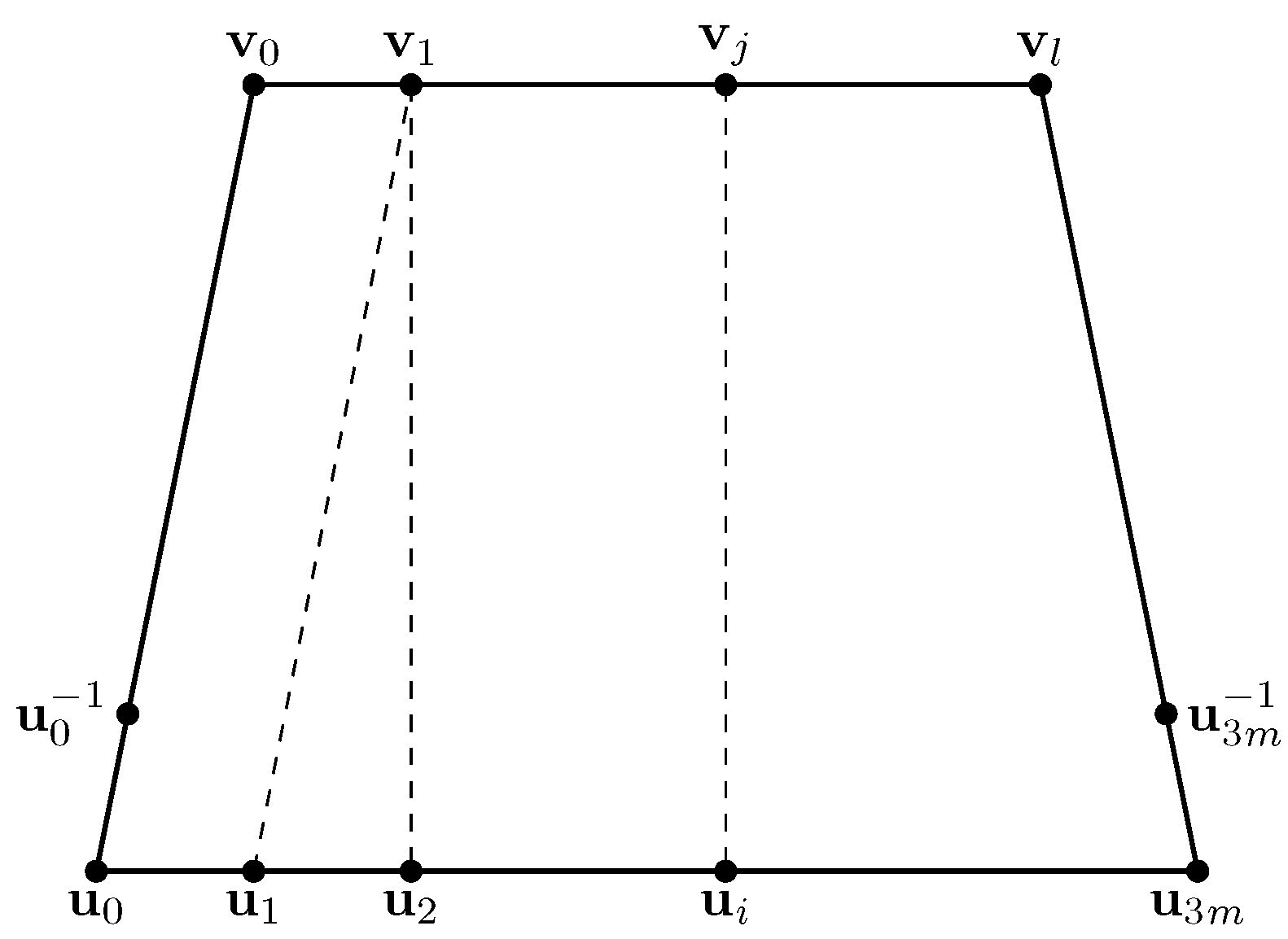
In general, the geodesic paths from
x to
y in an augmented tree
are not unique. However, there always exists a canonical geodesic of the following form:
where
are vertical paths; and
is a horizontal path (see
Figure 1). One or two parts may vanish in the canonical form. For any geodesic
, the distance from the root
o to the geodesics satisfy the following:
. Trivially, the Gromov product of
can be calculated as follows:
where
are the level and length of the horizontal part of the canonical geodesic
, respectively.
Lemma 1 ([
12])
. An augmented tree is a Gromov hyperbolic graph if and only if there exists such that the length of any horizontal geodesic is bounded by κ. A sequence
is called a geodesic ray and denoted by
, if
and
. It is useful to identify
with equivalent rays that converge to
. Two geodesic rays
and
are called equivalent [
19] if and only if there is
such that
for all but finitely many
n. Moreover, the Gromov product can be extended to the boundary
by assuming the following:
where
; and the infimum has taken over all geodesic rays
and
, converging to
and
, respectively.
Given an expansive matrix A with , the matrix A can define a pseudo-norm w on , which satisfies the following fundamental properties:
Proposition 1 ([
6])
. (i) and , where if and only if ;- (ii)
;
- (iii)
there is , such that for any , .
The
w induces a
w-distance, as follows:
It is easy to verify that
is a complete quasi-metric space [
20]. Moreover, we can define the
w-ball
; the
w-diameter of a set
; and the
w-distance between two sets
.
Let the IFS
be as in (
1); Proposition 1 (ii) tells us the following:
Hence, every
can be regarded as a contracting similitude with contraction ratio
in the quasi-metric space
. Let
and
be the symbolic space, where
. There is a natural tree structure on
by the standard concatenation of words, and we denote the edge set by
. That is,
if and only if there exists
such that
or
.
Let
K be the self-affine set as in (
2), and let
be as in the introduction. Then, we define a set of horizontal edges on
as follows:
where
is the contraction ratio of the IFS under quasi-metric
; and
is a constant.
Let . It follows from Definition 2 that the graph is an augmented tree induced by the IFS in the sense of Kaimanovich.
Lemma 2. Let the IFS as in (1). Suppose that the induced augmented tree is of bounded degree, then for any . Proof. If otherwise, there are
such that
. For any
, denote as follows:
Then,
for all
. Hence,
for all
, yielding that
This contradicts the assumption that
is of bounded degree. □
Lemma 3 ([
20]).
If the IFS in (1) satisfies the OSC, then we obtain the following:(*) for any , there exists such that for any , and any w-ball D with radius in , we have
3. Proof of Main Results
Theorem 5. The IFS in (1) satisfies the OSC if and only if the graph is of bounded degree. Proof. If the OSC holds, for any
with
, then
and
, where
. Let
D be a
w-ball, with the center at a point in
and the radius
. For any horizontal edge
, we have
and
. Hence,
. It follows from Lemma 3 that
Since
is an
N-ary tree, there are at most
terms
such that
is a vertical edge. Thus, the degree of
is as follows:
proving that
is of bounded degree.
On the contrary, first of all, we claim that the condition (*) in Lemma 3 is true. Otherwise, there is
; for any
, there is
and a
w-ball
D with radius
, as follows:
Let
and let
It follows that
Select a family of open ball sets
with radius
to cover
, where
is independent of
n and
is a constant in the definition of
. According to the pigeonhole principle, there exists a ball
that intersects at least
(the largest integer
) sets of
, say,
. This implies that, for any integers
,
. By (
6),
, hence
Since
can be sufficiently large,
can also be sufficiently large. It contradicts the assumption of bounded degree. We have proven the claim.
Finally, we show that the OSC is satisfied by constructing the desired open set. For the IFS in (
1), take an open ball
satisfying
. The above claim allows us to yield the following:
Hence, there are
for some
such that
and
’s are distinct. Let
It suffices to show that
U is the open set defining the OSC. Clearly,
is open and bounded and
. If the union is not disjointed, then there exists two distinct
such that
. From the definition of
U, it follows that there are
, which can be expressed as follows:
Without loss of generality, we may assume that the two words
lie in the same level, say
(otherwise, we can choose a prefix of the longer one).
It follows from Lemma 2 that the right-hand side set contains different functions, which contradicts the maximality of . We have completed the proof. □
In the absence of the OSC, we need to modify the graph as follows. First, we define a relation ∼ on the symbolic space . For , denote by if . Trivially, ∼ is an equivalence relation. Let be the quotient of and the equivalence class containing . In this situation, if and only if there exist and some , such that or . We call the quotient space of the graph . Subsequently, we still consider as for convenience. It should be mentioned that we have if the OSC holds.
Theorem 6. The IFS in (1) satisfies the WSC if and only if the quotient space is of bounded degree. Proof. The proof of sufficiency is analogous to that of Theorem 5, so we only need to show the necessity. For any
with
, then
. Let
be the
-neighborhood of
, as follows:
By the definition of horizontal edge set, for any
, we have
, that means
. It is easy to verify the following:
By (
3), we have the following:
For the vertical edges
, we have
or
, and
. By using (
3) again, we have the following:
Therefore, combining the horizontal and vertical edges, we can draw the following conclusion:
and
is of bounded degree. □
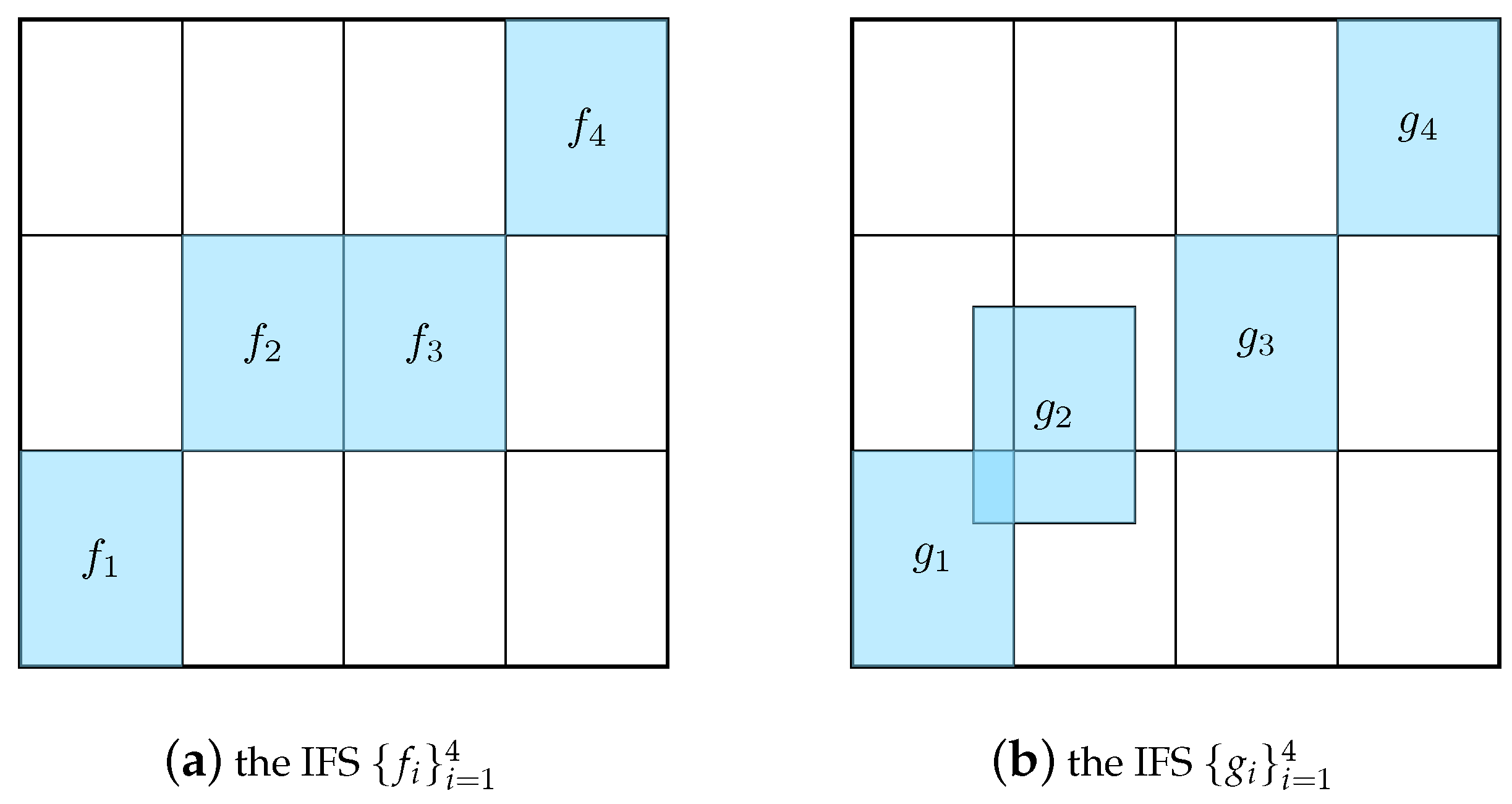
Example 1. Let , and be two digit sets as follows:Define one IFS as (see Figure 2a) and the other IFS as (see Figure 2b). It is easy to verify that the IFS satisfies the OSC by taking the interior of the unit square as the open set, and the graph as of bounded degree. In fact, for any vertex , the corresponding small rectangle intersects at most 8 rectangles with the same size; hence, by the definition of the augmented tree, has 1 father, 4 children, and at most 8 neighbors. Consequently, we have According to Theorem 2, we know that the IFS satisfies the WSC, but not the OSC. Hence, the graph is not of bounded degree by Theorem 5. It can also be verified immediately. For , we have (see Figure 2b). For any , let It follows that for any . Thus, the degree of the vertex is at least . Therefore, is not of bounded degree. On the other hand, if we consider as an equivalence class, i.e., a vertex in the quotient space . Theorem 6 implies that is of bounded degree.
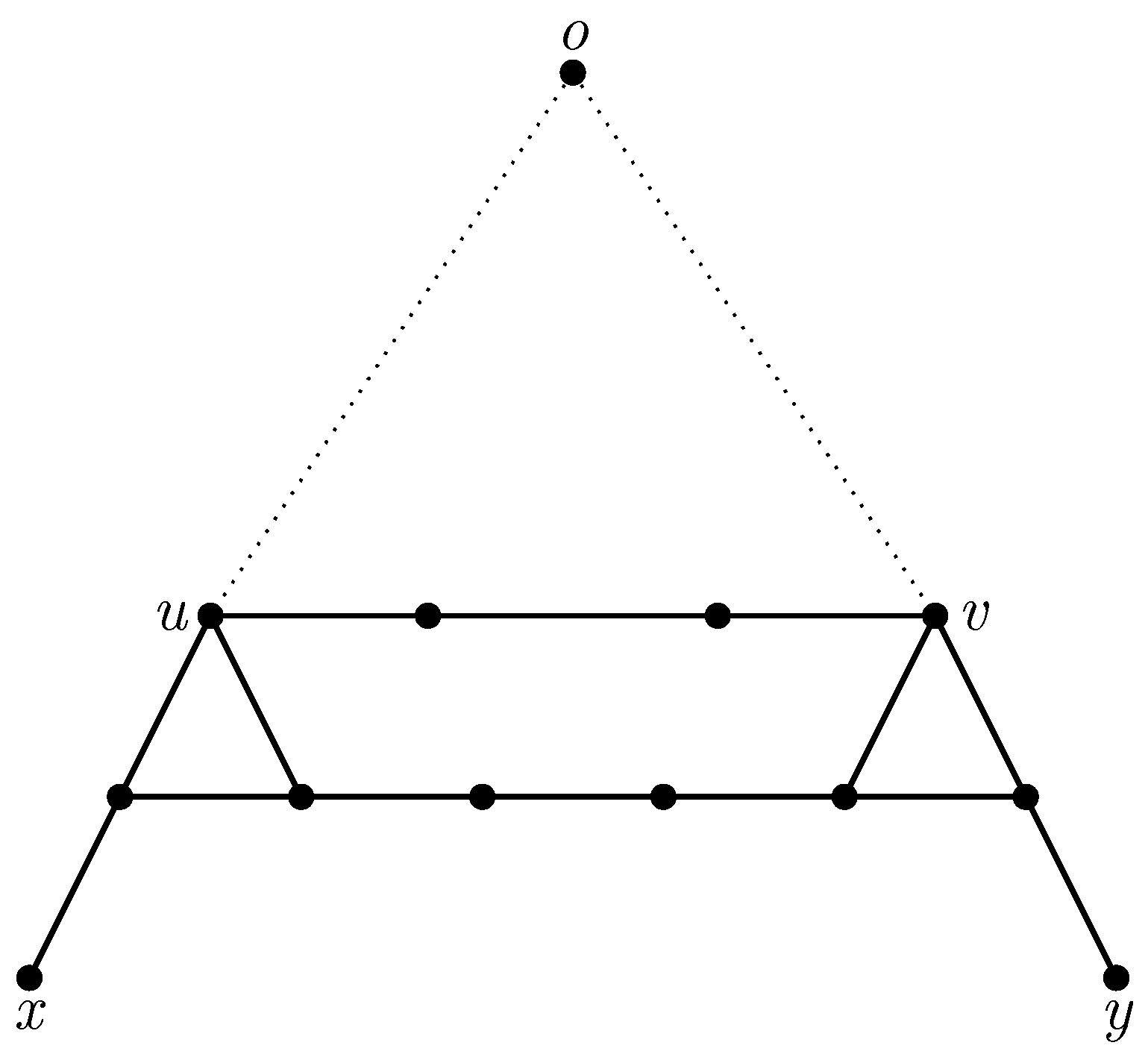
Proof of Theorem 4. We first prove that the graph
is a Gromov hyperbolic graph by contradiction. Suppose
G is not hyperbolic, then by Lemma 1, for any integer
, there exists a horizontal geodesic
with
for some
. The length of the geodesic is
. We can find another path
from
to
, where
o is the root of
G. It follows that
, then
. We consider the set
, which is the
m-th generation ancestor of
. Definition 2 implies that either
or
. Hence, there exists a shortest horizontal path, say,
, joining
and
, where
, and
(see
Figure 3). Therefore, we obtain a new path from
to
as follows:
By the property of geodesic, the length of path
is as follows:
Through the following:
we can estimate the
w-diameters of
E and
. Since
and
, we have
and
. Hence, we determine the following:
Since for any
, there is
i satisfying
, it follows that
, and
. Then, considering the following:
we can choose
m sufficiently large such that
. It is straightforward to obtain the following:
Let
, then there exists a ball
B with radius
such that
Let
and let
, the largest integer that is not greater than
. By assumption,
is the shortest horizontal path from
to
. Hence,
for any
. It follows that
, as well as the following:
By applying the pigeonhole principle, the ball
B contains at least
points
such that the
w-distance between any two of them is at least
. By (
7), we have
, which is impossible, as
m can be taken arbitrarily large. Hence, we have proven the hyperbolicity of
G.
For any point
, we let
be a geodesic ray representing
. Define a map
as follows:
for some
. The bijection of
follows from [
12] or [
14] immediately. It remains to verify the Hölder inequality (
4).
Let
be two different geodesic rays. There is a canonical bilateral geodesic
connecting
and
, as follows:
where
lie in the same level, say,
. Thus, we can deduce the following:
Note that for any
, we have :
which implies that
By making use of Proposition 1 (iii) twice, we can conclude the following:
where
is a constant.
By (
5) and (
9), the Gromov product
. Thus, we have the following:
By Lemma 1, the length
of the horizontal geodesic
is bounded by
. It implies that there is
, resulting in the following:
Hence, we determine the following:
where
.
On the other hand, it is clear that
. Then,
. Using (
10) again, there is
, allowing us to achieve the following:
Therefore, we obtain (
4) and complete the proof. □


