The Influence of Lévy Noise and Independent Jumps on the Dynamics of a Stochastic COVID-19 Model with Immune Response and Intracellular Transmission

Abstract

The coronavirus (COVID-19) expanded rapidly and affected almost the whole world since December 2019. COVID-19 has an unusual ability to spread quickly through airborne viruses and substances. Taking into account the disease’s natural progression, this study considers that viral spread is unpredictable rather than deterministic. The continuous time Markov chain (CTMC) stochastic model technique has been used to anticipate upcoming states using random variables. The suggested study focuses on a model with five distinct compartments. The first class contains Lévy noise-based infection rates (termed as vulnerable people), while the second class refers to the infectious compartment having similar perturbation incidence as the others. We demonstrate the existence and uniqueness of the positive solution of the model. Subsequently, we define a stochastic threshold as a requisite condition for the extinction and durability of the disease’s mean. By assuming that the threshold value ${\mathbf{R}}_{\mathbf{0}}^{\mathbf{D}}$ is smaller than one, it is demonstrated that the solution trajectories oscillate around the disease-free state (DFS) of the corresponding deterministic model. The solution curves of the SDE model fluctuate in the neighborhood of the endemic state of the base ODE system, when ${\mathbf{R}}_{\mathbf{0}}^{\mathbf{P}}>1$ elucidates the definitive persistence theory of the suggested model. Ultimately, numerical simulations are provided to confirm our theoretical findings. Moreover, the results indicate that stochastic environmental disturbances might influence the propagation of infectious diseases. Significantly, increased noise levels could hinder the transmission of epidemics within the community.

1. Introduction

The emerging virus at the end of 2019 is considered to be the most severe infectious disease, and the virologist community called it “Severe Acute Respiratory Syndrome Coronavirus-2 (SARS-CoV-2)” [1]. The disease is referred to as the virus-associated syndrome known as COVID-19. There was a unique strain of the coronavirus in humans known as SARS-CoV-2, which had not previously been discovered [2,3]. Many different animals may be infected with coronaviruses, and some of these species are particularly susceptible to infection by an individual. Among other animals, Bats are naturally believed to be the confirmed hosts of these new coronaviruses, but other animal species are also regarded to be a major contributor to their proliferation [4]. The recent infection, the MERS-CoV, an identical infection to COVID-19, spreads from camels to people. Civet cats are thought to be the source of SARS-CoV-1 for human transmission. For detailed analysis and explanation, the readers are suggested to see the ECDC fact-sheet on coronaviruses [4,5].

While animals have been recognized as a confirmed transmission route, human-to-human transfer is increasingly seen as a substantial element in the virus’s dissemination. Epidemiological data are currently insufficient for assessing the virus’s transmissibility among individuals. It is predicted that, on average, one infected individual may spread the virus to 2–3 others [1,5,6]. Cao et al. work on pan-cancer [7]. The virus is predominantly spread by small respiratory droplets emitted when an infected individual coughs, sneezes, or engages in close contact (often within three feet) with others for a certain duration. These droplets may be breathed directly or deposited on surfaces contacted by an infected individual, potentially leading to infection when others touch their mouth, nose, and/or eyes. The virus may persist on different surfaces for durations varying from a few hours (e.g., cardboard, copper) to several days (e.g., stainless steel, plastic). Nevertheless, the size of live virus progressively diminishes over time and may not persist at adequate levels to induce infection. The incubation time for COVID-19, defined as the interval between initial infection and symptom onset, is predicted to range from 1 to 14 days. Furthermore, as of the present date, no conclusive cure or vaccination exists. Scientists are expeditiously endeavoring to create a vaccine for the unique COVID-19; however, this process will require time. Consequently, the sole efficacious method to inhibit the transmission of the disease is to isolate and quarantine the originally affected individuals, as evidenced by the actions of the Chinese government and endorsed by WHO recommendations.

It is essential to recognize that the majority of real-world occurrences are not entirely deterministic. In models with no randomness, the output is solely dictated by the parameter’ value and beginning circumstances, yielding a singular, predictable result. Conversely, stochastic models integrate intrinsic unpredictability, indicating that identical parameter values and beginning conditions might provide a variety of distinct outcomes. A deterministic model uses numerical inputs to produce exact numerical outputs, whereas a stochastic model accommodates unpredictability in outcomes. A stochastic system contains a random element, utilizing a probability distribution as an input and generating a distribution for the output. These distributions may signify uncertainty in the input values (e.g., a deterministic input with superimposed noise) or embody an intrinsically random process (i.e., a stochastic input) [8,9,10].

Mathematical modeling is proven to be an effective instrument for accurately depicting the dynamic behavior of many epidemic illnesses. Throughout the years, various epidemic/dynamic models have been established by ecologists and mathematicians to comprehend and manage the dissemination of infectious illnesses across diverse locations. Over the last twenty years, mathematical modeling has been widely employed to elucidate the transmission dynamics of several infectious illnesses (see, e.g., [11,12]). Recently, substantial efforts have been undertaken to improve our comprehension of the new coronavirus (COVID-19), especially by extracting key insights using mathematical modeling. These models elucidate the dynamics of infectious illnesses. Stochastic differential equations are generally used for describing biological phenomena because they more accurately reflect intrinsic uncertainties and unpredictable changes. In contrast to deterministic models, stochastic models offer enhanced insights through many simulations, facilitating the development of a range of anticipated outcomes, such as the average number of infections at each specified time t. Conversely, deterministic models provide a singular predicted value [13,14,15,16]. Diverse methodologies have been established for the analysis of stochastic models [17,18].

Mathematical models play an important role in the control of disease. To enhance comprehension of COVID-19 transmission dynamics and its long-term behavior, the suggested model incorporates Lévy noises, hence introducing extra mathematical complexity. One of the main features of this model is that it recognizes the relationship between environmental contamination and disease and can identify the mechanisms by which people can become ill. These sounds provide benefits compared to ordinary Gaussian noises, especially in mathematical models connected to diseases. The incorporation of jump-diffusion Lévy noise is particularly important, since it elucidates the dynamics of neuronal membrane potential, rendering it a viable method for simulating intricate biological phenomena. Consequently, Lévy noise enhances the stabilization of time-varying neural networks. We examine the duration between the infection and manifestation of symptoms in an individual. The whole population of the community is divided into five mutually exclusive categories to more effectively analyze the illness dynamics. Subsequently, we will examine the prerequisites for disease extinction and stationary distribution, formulating adequate criteria for the propagation and management of COVID-19. Additionally, sample simulations will be performed utilizing the “Milstein scheme with jumps method” to corroborate and reinforce the theoretical results.

The arrangement for the remaining portions of the manuscript is as follows. The mathematical model that describes the dynamics of COVID-19 is proposed in Section 2, keeping in view the importance of Lévy noise and the underlying assumptions. The existence of a global positive solution and its uniqueness are investigated in Section 3. The essential prerequisites for the total extinction of the disease are outlined in Section 4. Section 5 goes into great length into the investigation of the infection’s persistence. In Section 6, we use graphical representations and numerical experiments to confirm the theoretical predictions. The study findings are compiled in Section 7 along with suggestions for more research.

2. Model Formulation

To formulate the model, we will extend the model of Rukhsar et al. [19] by incorporating the incidence rate. We introduce Lévy noise as a stochastic term in our model, where it plays a critical role in capturing the random fluctuations in the system. In our normalized population model, the total population is scaled to unity, meaning that each subpopulation (e.g., susceptible, infected) represents a fraction of the total population. We define excessive Lévy noise as a level of stochastic fluctuation that becomes significant compared to the size of the subpopulations. Since the total population is normalized, noise that exceeds the corresponding subpopulation levels can cause unmanageable fluctuations, leading to dynamics that may no longer be reflective of the real-world scenarios that the model aims to capture. To capture the dynamics of COVID-19, we will use five ordinary differential equations and initially, we formulate a deterministic mathematical model.

$$\begin{array}{cc}\hfill & \frac{d\mathbb{S}}{dt}=b-\frac{\beta \mathbb{S}\left(t\right)\mathbb{I}\left(t\right)\left(\delta \mathbb{I}\right(t)+1)}{\mathbb{N}\left(t\right)}-\left(\mu +d_3+\eta \right)\mathbb{S}\left(t\right),\hfill \\ \hfill & \frac{d\mathbb{E}}{dt}=\frac{\beta \mathbb{S}\left(t\right)\mathbb{I}\left(t\right)\left(\delta \mathbb{I}\right(t)+1)}{\mathbb{N}\left(t\right)}-\left(d_2+\lambda +\mu \right)\mathbb{E}\left(t\right),\hfill \\ \hfill & \frac{d\mathbb{I}}{dt}=\lambda \mathbb{E}\left(t\right)-\left(ϵ+d_1+\mu +\gamma \right)\mathbb{I}\left(t\right),\hfill \\ \hfill & \frac{d\mathbb{Q}}{dt}=d_2\mathbb{E}\left(t\right)+d_1\mathbb{I}\left(t\right)+d_3\mathbb{S}\left(t\right)-(\mu +\tau )\mathbb{Q}\left(t\right),\hfill \\ \hfill & \frac{d\mathbb{R}}{dt}=-\mu \mathbb{R}\left(t\right)+\eta \mathbb{S}\left(t\right)+\tau \mathbb{Q}\left(t\right)+\gamma \mathbb{I}\left(t\right).\hfill \end{array}$$

(1)

The threshold number ${\mathbf{R}}_{\mathbf{0}}^{\mathit{D}}$ for the given stochastic COVID-19 model can be derived using the next-generation matrix method.

$${\mathbf{R}}_{\mathbf{0}}^{\mathit{D}}=\frac{\beta \lambda (\delta +1)}{(\mu +d_3+\eta )(d_2+\lambda +\mu )(ϵ+d_1+\mu +\gamma )}.$$

(2)

The parameters and the description of the class in

Table 1. Model parameters and their descriptions.

Parameter	Description
$\mathbb{S}\left(t\right)$	The size of the vulnerable population at time t
$\mathbb{E}\left(t\right)$	Denote the size of the infected individuals at time t which are not yet infectious
$\mathbb{I}\left(t\right)$	Size of the infected compartment at time t
$\mathbb{Q}\left(t\right)$	At time t, the quarantined individuals
$\mathbb{R}\left(t\right)$	Recovered individuals at time t
b	Birth rate or recruitment into the susceptible population
$\beta$	Transmission rate of the infection
$\delta$	Modification factor accounting for enhanced transmission due to increased contact
$\mu$	Natural mortality rate
$d_1$	Rate of progression from infected to quarantined individuals
$d_2$	Rate of progression from exposed to quarantined individuals
$d_3$	Rate of direct transition from susceptible to quarantined individuals
$\eta$	Rate of natural immunity acquisition from susceptible individuals
$\lambda$	Rate of progression from exposed to infectious individuals
$ϵ$	Rate of disease-induced mortality in infected individuals
$\gamma$	Recovery rate from infection
$\tau$	Transition rate from quarantined to recovered individuals
$\mathbb{N}\left(t\right)$	Total number of individuals at any time t, defined as $\mathbb{N}\left(t\right)=\mathbb{S}\left(t\right)+\mathbb{E}\left(t\right)+\mathbb{I}\left(t\right)+\mathbb{Q}\left(t\right)+\mathbb{R}\left(t\right)$

.

It is critically noticed that, regardless of how many variables and parameters you include within the model, differences still exist between the real-world phenomenon and those results predicted by the model. The same is the case with epidemics, as several environmental fluctuations may affect the dynamics of the disease, for example, earthquakes, tsunamis, and weather. These fluctuations could directly disrupt the continuity of the solution and thus the traditional white noises are unable to accurately predict the model behavior. Studies suggest that, in such cases, the inclusion of Lévy jumps into the epidemic models is the best and an effective approach [20]. To control an epidemic and to help in the prevention of the disease, Lévy noise could play a crucial role as it has the ability to explain the intrinsic dynamics of infectious diseases. In this work, the study already conducted in [21] was further extended by including the Lévy noises and vaccination as a control measure. The deterministic model (1) will take the following stochastic form:

$$\begin{array}{cc}\hfill d\mathbb{S}\left(t\right)& =\left[b-\frac{\beta \mathbb{S}\left(t\right)\mathbb{I}\left(t\right)\left(\delta \mathbb{I}\right(t)+1)}{\mathbb{N}\left(t\right)}-\left(\mu +d_3+\eta \right)\mathbb{S}\left(t\right)\right]dt+{\delta }_1\mathbb{S}\left(t\right)d{\mathbb{W}}_1\left(t\right)+{\int }_{\mathbb{X}}{\mathbb{Z}}_1\left(x\right)\mathbb{S}\left(t^{-}\right)\tilde{S}\left(d\zeta \right),\hfill \\ \hfill d\mathbb{E}\left(t\right)& =\left[\frac{\beta \mathbb{S}\left(t\right)\mathbb{I}\left(t\right)\left(\delta \mathbb{I}\right(t)+1)}{\mathbb{N}\left(t\right)}-\left(d_2+\lambda +\mu \right)\mathbb{E}\left(t\right)\right]dt+{\delta }_2\mathbb{E}\left(t\right)d{\mathbb{W}}_2\left(t\right)\hfill \\ \hfill & +{\int }_{\mathbb{X}}{\mathbb{Z}}_2\left(x\right)\mathbb{E}\left(t^{-}\right)\tilde{S}\left(d\zeta \right),\hfill \\ \hfill d\mathbb{I}\left(t\right)& =\left[\lambda \mathbb{E}\left(t\right)-\left(ϵ+d_1+\mu +\gamma \right)\mathbb{I}\left(t\right)\right]dt+{\delta }_3\mathbb{I}\left(t\right)d{\mathbb{W}}_3\left(t\right)+{\int }_{\mathbb{X}}{\mathbb{Z}}_3\left(x\right)\mathbb{I}\left(t^{-}\right)\tilde{S}\left(d\zeta \right),\hfill \\ \hfill d\mathbb{Q}\left(t\right)& =\left[d_2\mathbb{E}\left(t\right)+d_1\mathbb{I}\left(t\right)+d_3\mathbb{S}\left(t\right)-(\tau +\mu )\mathbb{Q}\left(t\right)\right]dt+{\delta }_4\mathbb{Q}\left(t\right)d{\mathbb{W}}_4\left(t\right)+{\int }_{\mathbb{X}}{\mathbb{Z}}_4\left(x\right)\mathbb{Q}\left(t\right)\left(t^{-}\right)\tilde{S}\left(d\zeta \right),\hfill \\ \hfill d\mathbb{R}\left(t\right)& =\left[\eta \mathbb{S}\left(t\right)+\gamma \mathbb{I}\left(t\right)+\tau \mathbb{Q}\left(t\right)-\mu \mathbb{R}\left(t\right)\right]dt+{\delta }_5\mathbb{R}\left(t\right)d{\mathbb{W}}_4\left(t\right)+{\int }_{\mathbb{X}}{\mathbb{Z}}_5\left(x\right)\mathbb{R}\left(t\right)\left(t^{-}\right)\tilde{S}\left(d\zeta \right),\hfill \end{array}$$

(3)

where $\left(d\zeta \right)=(dt,dx)$.

The time-dependent functions ${\mathbb{W}}_i\left(t\right)$ for $i=1,2,3,4,5$ stand for the Brownian motions which are defined on a complete probability space $(\Omega ,\mathbb{F},\P )$ having $\mathbb{F}\ge 0$ as a filtration, which satisfies the trivial supposition, i.e., it is an increasing function and right-continuity holds for all ¶-empty sets; ${\alpha }_i(i=1,\dots ,4)$ represents the intensity of white noise. Where $\mathbb{S}\left(t^{-}\right),\mathbb{E}\left(t^{-}\right),\mathbb{I}\left(t^{-}\right),\mathbb{Q}\left(t^{-}\right)$ and $\mathbb{R}\left(t^{-}\right)$ are the left limit of $\mathbb{S}\left(t\right),\mathbb{E}\left(t\right),\mathbb{I}\left(t\right),\mathbb{Q}\left(t\right)$ and $\mathbb{R}\left(t\right)$, respectively, $\tilde{S}\left(d{\zeta }_1\right)$, N is a Poisson counting measure with a characteristic measure x on measurable subset $\mathbb{X}$ of $[0,\infty )$, with $v\left(\mathbb{X}\right)<\infty$, and ${\mathbb{Z}}_i:\mathbb{X}\times \Omega ⟶\mathbb{R}(i=1,2,3,4,5)$ represent the effects.

3. Existence and Uniqueness

We now emphasize that the system (3) has the existence and uniqueness of the solution. Let us define some assumptions and Lemmas in the stochastic sense.

$$\begin{array}{c}\hfill {\displaystyle \langle \mathcal{G}\left(t\right)\rangle =\frac{1}{t}{\int }_0^t\mathcal{G}\left(x\right)dx.}\end{array}$$

The two standard assumptions, $\left({\mathbb{G}}_1\right)$ and $\left({\mathbb{G}}_2\right)$, are essential for proving the existence and uniqueness of a global positive solution to (3).

Lemma 1.

$\left({\mathbb{G}}_1\right)$.

$\forall \mathbb{M}>0\exists {\mathbb{L}}_{\mathbb{M}}>0$ such that

$${\int }_{\mathbb{Y}}{\left|{\mathbb{Z}}_i\left(y_1,x\right)-{\mathbb{Z}}_i\left(y_2,x\right)\right|}^{2}v\left(dy\right)\le {\mathbb{L}}_{\mathbb{M}}{\left|x_1-x_2\right|}^2,i=1,2,3,4,5,$$

(4)

with $\left|x_1\right|\vee \left|x_2\right|\le \mathbb{M}$, where

$$\begin{array}{cc}\hfill {\mathbb{Z}}_1(x,s)& ={\Omega }_1\left(s\right)x\mathrm{for}x=\mathbb{S}\left(t^{-}\right),\hfill \\ \hfill {\mathbb{Z}}_2(x,s)& ={\Omega }_2\left(s\right)x\mathrm{for}x=\mathbb{E}\left(t^{-}\right),\hfill \\ \hfill {\mathbb{Z}}_3(x,s)& ={\Omega }_3\left(s\right)x\mathrm{for}x=\mathbb{I}\left(t^{-}\right),\hfill \\ \hfill {\mathbb{Z}}_4(x,s)& ={\Omega }_4\left(s\right)x\mathrm{for}x=\mathbb{Q}\left(t^{-}\right),\hfill \\ \hfill {\mathbb{Z}}_5(x,s)& ={\Omega }_5\left(s\right)x\mathrm{for}x=\mathbb{R}\left(t^{-}\right).\hfill \end{array}$$

(5)

where $\mathbb{Z}$ denotes the compensated random measure.

$\left({\mathbb{G}}_2\right)$.

$\left|\log \left(1+{\Omega }_i\left(x\right)\right)\right|\le C$ for ${\Omega }_i\left(x\right)>-1,{\Omega }_i=1,2,3,4,5$ where C is a positive constant.

Theorem 1.

There is a unique solution $\left(\mathbb{S}\right(t),\mathbb{E}(t),\mathbb{I}(t),\mathbb{Q}(t),\mathbb{R}(t\left)\right)$ of system (3) on t with initial value $\left(\mathbb{S}\right(0),\mathbb{E}(0),\mathbb{I}(0),\mathbb{Q}(0),\mathbb{R}(0\left)\right)$ for any $R_5^{+}$, and the solution will remain in $R_5^{+}$ with probability one, namely $(\mathbb{S}\left(t\right),\mathbb{E}\left(t\right),\mathbb{I}\left(t\right),\mathbb{Q}\left(t\right),\mathbb{R}\left(t\right))\in R_5^{+}$ for all $t\ge 0$ almost surely.

Proof. 

The system (3) is locally Lipschitz, resulting in a time t during which the proposed problem has a locally unique solution within the interval $[0,{\tau }_e)$. The condition $\left({\mathbb{G}}_{!}\right)$ for any $\left(\mathbb{S}\right(0),\mathbb{E}(0),\mathbb{I}(0),\mathbb{Q}(0),\mathbb{R}(0\left)\right)$ for any $R_5^{+}$, the coefficients of our model accurately fulfill the Lipschitz local criterion. Consequently, $\left(\mathbb{S}\right(t),\mathbb{E}(t),\mathbb{I}(t),\mathbb{Q}(t),\mathbb{R}(t\left)\right)$ represents a unique local solution for $t\in [0,e)$, where e denotes the explosion time. We shall now demonstrate that the solution is still globally valid and establish $e=\infty$ almost surely. When $k_0$ is large enough to ensure that $k_0\to 0$, the starting approximation $\mathbb{S}\left(0\right),\mathbb{E}\left(0\right),\mathbb{I}\left(0\right),\mathbb{Q}\left(0\right)$ and $\mathbb{R}\left(0\right)$ are in $\left[\frac{1}{k_0},k_0\right]$. We calculate the stopping time for $k\ge k_0$, as

$$\begin{array}{c}\hfill {\tau }_k=\inf \left\{t\in [0,{\tau }_e):\max (\mathbb{S}\left(t\right),\mathbb{E}\left(t\right),\mathbb{I}\left(t\right),\mathbb{Q}\left(t\right),\mathbb{R}\left(t\right))\ge k\mathrm{or}\min (\mathbb{S}\left(t\right),\mathbb{E}\left(t\right),\mathbb{I}\left(t\right),\mathbb{Q}\left(t\right),\mathbb{R}\left(t\right))\le \frac{1}{k}\right\}.\end{array}$$

(6)

In this study, we employ the concept of $\inf \varnothing =\infty$, where ∅ represents the null set, in accordance with the work of [20,21,22,23]. Since k increases whenever k approaches ∞, thus, ${\lim }_{k\to \infty }k=\infty$ along the application of ${\tau }_{\infty }\le {\tau }_e$ almost surely, showing that ${\tau }_{\infty }=\infty$ almost surely. Accordingly, this will ensure that the solution of model (3) lies in $R_5^{+}$ almost surely for $t\ge 0$. To show that ${\tau }_{\infty }=\infty$ almost surely, if this statement is not correct, then there exist a pair of constants $T>0$ and $ϵ\in (0,1)$ such that

$$P\{{\tau }_{\infty }\le T\}>ϵ.$$

As a result, there is an integer $k_1>k_0$ such that $P(T_k>k_1)=k$.

Consider a $C^2$-mapping $H:R_5^{+}\to \overline{R_{+}}$, where $\overline{R_{+}}=\{x\in R:x\ge 0\}$.

$$\begin{array}{cc}\hfill H(\mathbb{S},\mathbb{E},\mathbb{I},\mathbb{R},\mathbb{Q})& =(\mathbb{S}-\ln \mathbb{S}-1)+(\mathbb{I}-\ln \mathbb{I}-1)+(\mathbb{E}-\ln \mathbb{E}-1)\hfill \\ \hfill & +(\mathbb{R}-\ln \mathbb{R}-1)+(\mathbb{Q}-\ln \mathbb{Q}-1).\hfill \end{array}$$

(7)

Using the Itô formula in Equation (7) gives us

$$\begin{array}{cc}\hfill LH(\mathbb{S},\mathbb{E},\mathbb{I},\mathbb{R},\mathbb{Q})& =LHdt+{\delta }_1(\mathbb{S}-1)d{W}_1\left(t\right)+{\delta }_2(\mathbb{E}-1)d{W}_2\left(t\right)+{\delta }_3(\mathbb{I}-1)d{W}_3\left(t\right)\hfill \\ & +{\delta }_4(\mathbb{Q}-1)d{W}_4\left(t\right)+{\delta }_5(\mathbb{R}-1)d{W}_5\left(t\right)+{\int }_{\mathbb{X}}[{\mathbb{Z}}_1\left(x\right)\mathbb{S}-\ln (1+{\mathbb{Z}}_1\left(x\right))]\tilde{S}\left(d\zeta \right)\hfill \\ & +{\int }_{\mathbb{X}}[{\mathbb{Z}}_2\left(x\right)\mathbb{E}-\ln (1+{\mathbb{Z}}_2\left(x\right))]\tilde{S}\left(d\zeta \right)+{\int }_{\mathbb{X}}[{\mathbb{Z}}_3\left(x\right)\mathbb{I}-\ln (1+{\mathbb{Z}}_3\left(x\right))]\tilde{S}\left(d\zeta \right)\hfill \\ & +{\int }_{\mathbb{X}}[{\mathbb{Z}}_4\left(x\right)\mathbb{R}-\ln (1+{\mathbb{Z}}_4\left(x\right))]\tilde{S}\left(d\zeta \right)+{\int }_{\mathbb{X}}[{\mathbb{Z}}_5\left(x\right)\mathbb{Q}-\ln (1+{\mathbb{Z}}_5\left(x\right))]\tilde{S}\left(d\zeta \right).\hfill \end{array}$$

(8)

Thus, in Equation (8), $LH:R_5^{+}\to R_{+}$, and we can write

$$\begin{array}{cc}\hfill LH& =\left(1-\frac{1}{\mathbb{S}}\right)\left(b-\frac{\beta \mathbb{S}\left(t\right)\mathbb{I}\left(t\right)\left(\delta \mathbb{I}\right(t)+1)}{\mathbb{N}\left(t\right)}-\left(\mu +d_3+\eta \right)\mathbb{S}\left(t\right)\right)+\frac{{\delta }_1^2}{2}\hfill \\ & +{\int }_{\mathbb{X}}[{\mathbb{Z}}_1\left(x\right)-\ln (1+{\mathbb{Z}}_1\left(x\right))]\tilde{S}\left(d\zeta \right)\hfill \\ & +\left(1-\frac{1}{\mathbb{E}}\right)\left(\frac{\beta \mathbb{S}\left(t\right)\mathbb{I}\left(t\right)\left(\delta \mathbb{I}\right(t)+1)}{\mathbb{N}\left(t\right)}-\left(d_2+\lambda +\mu \right)\mathbb{E}\left(t\right)\right)+\frac{{\delta }_2^2}{2}\hfill \\ & +{\int }_{\mathbb{X}}[{\mathbb{Z}}_2\left(x\right)-\ln (1+{\mathbb{Z}}_2\left(x\right))]\tilde{S}\left(d\zeta \right)\hfill \\ & +\left(1-\frac{1}{\mathbb{I}}\right)\left(\lambda \mathbb{E}\left(t\right)-\left(ϵ+d_1+\mu +\gamma \right)\mathbb{I}\left(t\right)\right)+\frac{{\delta }_3^2}{2}\hfill \\ & +{\int }_{\mathbb{X}}[{\mathbb{Z}}_3\left(x\right)-\ln (1+{\mathbb{Z}}_3\left(x\right))]\tilde{S}\left(d\zeta \right)\hfill \\ & +\left(1-\frac{1}{\mathbb{R}}\right)\left(\eta \mathbb{S}\left(t\right)+\gamma \mathbb{I}\left(t\right)+\tau \mathbb{Q}\left(t\right)-\mu \mathbb{R}\left(t\right)\right)+\frac{{\delta }_4^2}{2}\hfill \\ & +{\int }_{\mathbb{X}}[{\mathbb{Z}}_4\left(x\right)-\ln (1+{\mathbb{Z}}_4\left(x\right))]\tilde{S}\left(d\zeta \right)\hfill \\ & +\left(1-\frac{1}{\mathbb{Q}}\right)\left(\eta \mathbb{S}\left(t\right)+\gamma \mathbb{I}\left(t\right)+\tau \mathbb{Q}\left(t\right)-\mu \mathbb{R}\left(t\right)\right)+\frac{{\delta }_5^2}{2}\hfill \\ & +{\int }_{\mathbb{X}}[{\mathbb{Z}}_5\left(x\right)-\ln (1+{\mathbb{Z}}_5\left(x\right))]\tilde{S}\left(d\zeta \right).\hfill \end{array}$$

(9)

Then

$$\begin{array}{cc}\hfill LH& =b-\mu (\mathbb{S}+\mathbb{E}+\mathbb{I}+\mathbb{Q}+\mathbb{R})-ϵ\mathbb{I}-\frac{b}{\mathbb{S}}+\frac{\beta \mathbb{I}(\delta +1)}{\mathbb{N}}+(\eta +d_3+\mu )\hfill \\ \hfill & -\frac{\beta \mathbb{S}\mathbb{I}(\delta \mathbb{I}+1)}{\mathbb{E}\mathbb{N}}+(\lambda +\mu +d_2)-\frac{\lambda \mathbb{E}}{\mathbb{I}}+(\mu +ϵ+\gamma +d_1)-\frac{d_2\mathbb{E}}{\mathbb{Q}}\hfill \\ & -\frac{d_3\mathbb{S}}{\mathbb{Q}}-\frac{d_1\mathbb{I}}{\mathbb{Q}}+(\tau +\mu )-\frac{\tau \mathbb{Q}}{\mathbb{R}}-\frac{\gamma \mathbb{I}}{\mathbb{R}}+\sum _{i=1}^5\frac{{\delta }_i^2}{2}\hfill \\ \hfill & +\sum _{i=1}^5{\int }_{\mathbb{X}}{\mathbb{Z}}_i\left(x\right)\tilde{S}\left(d\zeta \right)-\sum _{i=1}^5{\int }_{\mathbb{X}}\ln ({\mathbb{Z}}_i\left(x\right)+1)\tilde{S}\left(d\zeta \right)\hfill \\ \hfill & \le b+\beta (1+\delta )+\eta +5\mu +d_3+\lambda +d_2+ϵ+\gamma +d_1+\tau \hfill \\ \hfill & +\sum _{i=1}^5\frac{{\delta }_i^2}{2}+\sum _{i=1}^5{\int }_{\mathbb{X}}{\mathbb{Z}}_i\left(x\right)\tilde{S}\left(d\zeta \right)-\sum _{i=1}^5{\int }_{\mathbb{X}}\ln ({\mathbb{Z}}_i\left(x\right)+1)\tilde{S}\left(d\zeta \right):=\mathbb{K}.\hfill \end{array}$$

(10)

The remainder of the proof closely follows the methodology outlined in the study [20]; therefore, to avoid redundancy, we omit the detailed steps here. □

4. Extinction

Mitigating the long-term effects of a disease in a society necessitates the identification of certain circumstances through the examination of the epidemic’s dynamic behavior. Comprehending these circumstances is essential for formulating effective management methods and forecasting illness development. This section analyzes the fundamental conditions for disease elimination via a stochastic modeling technique. To provide a definitive framework, we initially delineate the essential notations as follows:

$$x\left(t\right)=\frac{1}{t}{\int }_0^{t}x\left(s\right)ds.$$

Lemma 2.

If problem (3), $(\mathbb{S},\mathbb{E},\mathbb{I},\mathbb{R},\mathbb{Q})$ is a root with the initial approximation $({\mathbb{S}}_0,{\mathbb{E}}_0,{\mathbb{I}}_0,{\mathbb{R}}_0,{\mathbb{Q}}_0)\in R_{+}^5$, then almost surely (a.s.),

$$\underset{t\to \infty }{\lim }\frac{\mathbb{S}\left(t\right)+\mathbb{E}\left(t\right)+\mathbb{I}\left(t\right)+\mathbb{R}\left(t\right)+\mathbb{Q}\left(t\right)}{t}=0.$$

Further, if

$$q>\frac{{\delta }_1^2\vee {\delta }_2^2\vee {\delta }_3^2\vee {\delta }_4^2\vee {\delta }_5^2}{2},$$

then

$$\underset{t\to \infty }{\lim }\frac{1}{t}{\int }_0^t\mathbb{S}\left(r\right)d{\mathbb{W}}_1\left(r\right)=0,\underset{t\to \infty }{\lim }\frac{1}{t}{\int }_0^t\mathbb{E}\left(r\right)d{\mathbb{W}}_2\left(r\right)=0,$$

$$\underset{t\to \infty }{\lim }\frac{1}{t}{\int }_0^t\mathbb{I}\left(r\right)d{\mathbb{W}}_3\left(r\right)=0,\underset{t\to \infty }{\lim }\frac{1}{t}{\int }_0^t\mathbb{Q}\left(r\right)d{\mathbb{W}}_4\left(r\right)=0,$$

$$\underset{t\to \infty }{\lim }\frac{1}{t}{\int }_0^t\mathbb{R}\left(r\right)d{\mathbb{W}}_5\left(r\right)=0.$$

Proof. 

The derivation of the aforementioned result is omitted, as the ultimate conclusions may be derived using the methods detailed in the proofs of Lemmas (2.1) and (2.2) in Zhao and Jiang [24]. Alternatively, a comprehensive proof is available in [25]. □

Theorem 2.

Let $\mu >\left(\frac{1}{2}\right)\left({\delta }_1^2\vee {\delta }_2^2\vee {\delta }_3^2\vee {\delta }_4^2\vee {\delta }_5^2\right)$ then $(\mathbb{S}\left(0\right),\mathbb{E}\left(0\right),\mathbb{I}\left(0\right),\mathbb{R}\left(0\right),\mathbb{Q}\left(0\right))\in {\mathbb{R}}_{+}^5$ and if

$${\mathbf{R}}_{\mathbf{0}}^{\mathit{E}}=\frac{2\lambda \beta (1+\sigma )(\lambda +\mu +d_2)}{\left(d_2+\mu +ϵ+\gamma +\frac{{\delta }_3^2}{2}+{\int }_{\mathbb{X}}[{\mathbb{Z}}_3\left(x\right)+\ln (1+{\mathbb{Z}}_3\left(x\right))]vd\left(x\right)\right){\left(d_2+\lambda +\mu \right)}^2\wedge \left({\lambda }^2\frac{{\delta }_2^2}{2}\right)}.$$

hold, then

$$\underset{t\to \infty }{\lim }\mathbb{I}\left(t\right)=0,\underset{t\to \infty }{\lim }\mathbb{E}\left(t\right)=0\mathrm{as}t\to \infty .$$

Moreover,

$$\underset{t\to \infty }{\lim }\langle \mathbb{S}\rangle =\frac{b}{\eta +\mu +d_3},$$

$$\underset{t\to \infty }{\lim }\langle \mathbb{Q}\rangle =\frac{b{d}_3}{(\eta +\mu +d_3)(\mu +\tau )},$$

$$\underset{t\to \infty }{\lim }\langle \mathbb{R}\rangle =\frac{b(\eta (\mu +\tau )+\tau d_3)}{\mu (\eta +\mu +d_3)(\mu +\tau )},a.s.$$

Proof. 

Define a function $W_0$ which is differentiable as follows:

$$W_0=\ln \left[\left(\mu +\lambda +d_2\right)\mathbb{I}\left(t\right)+\lambda \mathbb{E}\left(t\right)\right].$$

According to Itô’s formula and model (3), we acquire

$$\begin{array}{cc}\hfill d{W}_0& =\left\{\frac{\beta \lambda \mathbb{S}\mathbb{I}(1+\delta \mathbb{I})}{\mathbb{N}[\lambda \mathbb{E}\left(t\right)+(\mu +\lambda +d_2)\mathbb{I}\left(t\right)]}+\frac{(\mu +\lambda +d_2)(ϵ+\mu +\gamma +d_1)}{\mathbb{N}[(\mu +\lambda +d_2)\mathbb{I}\left(t\right)+\lambda \mathbb{E}\left(t\right)]}-\lambda \frac{{\delta }_2^2{\lambda }^2{\mathbb{E}}^2+(\mu +\lambda +d_2){\delta }_3^2{\mathbb{I}}^2}{2({(\lambda \mathbb{E}\left(t\right)+(\lambda +\mu +d_2)\mathbb{I}\left(t\right))}^2}\right\}dt\hfill \\ \hfill & +\frac{\lambda {\delta }_2\mathbb{E}}{(\mu +\lambda +d_2)\mathbb{I}\left(t\right)+\lambda \mathbb{E}\left(t\right)}d{\mathbb{W}}_2+\frac{(\mu +\lambda +d_2){\delta }_3\mathbb{I}\left(t\right)}{\lambda \mathbb{E}\left(t\right)+((\mu +\lambda +d_2)\mathbb{I}\left(t\right)+\lambda \mathbb{E}\left(t\right))}d{\mathbb{W}}_3\hfill \\ \hfill & +\frac{\lambda (-{\int }_{\mathbb{X}}\left[{\mathbb{Z}}_2\left(x\right)-\log \left(1+{\mathbb{Z}}_2\left(x\right)\right)\right]v\left(dx\right)+{\int }_{\mathbb{Z}}\left[\log \left({\mathbb{Z}}_2\left(x\right)+1\right)\right])}{\lambda \mathbb{E}\left(t\right)+(\mu +\lambda +d_2)\mathbb{I}\left(t\right)]}\hfill \\ \hfill & +\frac{(\mu +\lambda +d_2)(-{\int }_{\mathbb{X}}\left[{\mathbb{Z}}_3\left(x\right)-\log \left(1+{\mathbb{Z}}_3\left(x\right)\right)\right]v\left(dx\right)+{\int }_{\mathbb{Z}}\left[\log \left({\mathbb{Z}}_3\left(x\right)+1\right)\right])}{(\mu +\lambda +d_2)\mathbb{I}\left(t\right)+\lambda \mathbb{E}\left(t\right)}\hfill \\ & =\left\{\frac{\lambda \beta (1+\sigma \mathbb{I})}{(\lambda +\mu +d_2)}-\frac{(\mu +ϵ+\gamma +d_2+\frac{{\delta }_3^2}{2}+{\int }_{\mathbb{X}}[{\mathbb{Z}}_3\left(x\right)+\ln (1+{\mathbb{Z}}_3\left(x\right))]vd\left(x\right)){(\lambda +\mu +d_2)}^2{\mathbb{I}}^2+\left({\lambda }^2\frac{{\delta }_2^2}{2}{\mathbb{E}}^2\right)}{{(\lambda \mathbb{E}\left(t\right)+(d_2+\lambda +\mu )\mathbb{I}\left(t\right))}^2}\right\}dt\hfill \\ & +\frac{\lambda {\delta }_2\mathbb{E}}{\lambda \mathbb{E}\left(t\right)+(\lambda +\mu +d_2)\mathbb{I}\left(t\right)}d{\mathbb{W}}_2+\frac{(\lambda +\mu +d_2){\delta }_3\mathbb{I}\left(t\right)}{\lambda \mathbb{E}\left(t\right)+(\lambda \mathbb{E}\left(t\right)+(\lambda +\mu +d_2)\mathbb{I}\left(t\right)}d{\mathbb{W}}_3\hfill \\ & \\ & =\left\{\frac{\lambda \beta (1+\sigma \mathbb{I})}{(\lambda +\mu +d_2)}-\frac{(\mu +ϵ+\gamma +d_2+\frac{{\delta }_3^2}{2}+{\int }_{\mathbb{X}}[{\mathbb{Z}}_3\left(x\right)+\ln (1+{\mathbb{Z}}_3\left(x\right))]vd\left(x\right)){(\lambda +\mu +d_2)}^2\wedge \left({\lambda }^2\frac{{\delta }_2^2}{2}\right)}{{(\lambda \mathbb{E}\left(t\right)+(d_2+\lambda +\mu )\mathbb{I}\left(t\right))}^2}\right\}dt\hfill \\ & +\frac{\lambda {\delta }_2\mathbb{E}}{\lambda \mathbb{E}\left(t\right)+(\lambda +\mu +d_2)\mathbb{I}\left(t\right)}d{\mathbb{W}}_2+\frac{(\lambda +\mu +d_2){\delta }_3\mathbb{I}\left(t\right)}{\lambda \mathbb{E}\left(t\right)+(\lambda \mathbb{E}\left(t\right)+(\lambda +\mu +d_2)\mathbb{I}\left(t\right)}d{\mathbb{W}}_3.\hfill \end{array}$$

(11)

Divide both sides of Equation (11) by t and integrate from 0 to t. Also, by Lemma 2, we have

$$\begin{array}{cc}\hfill \lim \underset{t\to \infty }{\sup }& \frac{\ln \left[\delta \mathbb{E}\right(t)+(\delta +\mu \left)\mathbb{I}\right(t\left)\right]}{t}\le \frac{\lambda \beta (1+\delta )}{\lambda +\mu +d_2}\hfill \\ & -\frac{(\mu +ϵ+\gamma +d_2+\frac{{\delta }_3^2}{2}+{\int }_{\mathbb{X}}[{\mathbb{Z}}_3\left(x\right)+\ln (1+{\mathbb{Z}}_3\left(x\right))]vd\left(x\right)){(\lambda +\mu +d_2)}^2\wedge \left({\lambda }^2\frac{{\delta }_2^2}{2}\right)}{2{(d_2+\lambda +\mu )}^2}<0a.s.\hfill \end{array}$$

(12)

which illustrates that

$$\underset{t\to \infty }{\lim }\mathbb{I}\left(t\right)=0,\underset{t\to \infty }{\lim }\mathbb{E}\left(t\right)=0\mathrm{as}t\to \infty .$$

Furthermore, the first equation of system (3) can be divided by t on both sides and integrated from 0 to t to obtain a solution.

$$\frac{\mathbb{S}\left(t\right)-\mathbb{S}\left(0\right)}{t}=b-\beta \langle \frac{\mathbb{S}\mathbb{I}}{\mathbb{N}}\rangle -(\eta +\mu +d_3)\langle \mathbb{S}\rangle +\frac{{\delta }_1}{t}{\int }_0^t\mathbb{S}\left(r\right)d{\mathbb{W}}_1\left(r\right)+\frac{1}{t}{\int }_0^t\left[{\int }_{\mathbb{X}}{\mathbb{Z}}_1\left(x\right)\mathbb{S}\left(t^{-}\right)\tilde{S}\left(d\zeta \right)\right]dr,$$

using Lemma 2, then we can obtain.

$$\underset{t\to \infty }{\lim }\langle \mathbb{S}\rangle =\frac{b}{\eta +\mu +d_3},$$

$$\underset{t\to \infty }{\lim }\langle \mathbb{Q}\rangle =\frac{b{d}_3}{(\eta +\mu +d_3)(\mu +\tau )},$$

$$\underset{t\to \infty }{\lim }\langle \mathbb{R}\rangle =\frac{b(\eta (\mu +\tau )+\tau d_3)}{\mu (\eta +\mu +d_3)(\mu +\tau )},a.s.$$

The proof for Theorem 2 has been completed. □

5. Persistence

This section examines the long-term effects of the disease through an analysis of its temporal persistence. To construct a robust theoretical foundation, we initially define persistence in the average, as presented by Khan et al. [23]. This definition will provide a base for comprehending the enduring consequences of the infection and its possible repercussions.

Definition 1.

Zhao and Jiang [24] suggested the subsequent assumption to tackle the system’s persistence and long-term effects of the disease whose dynamics are governed by (3): The limit is inferior as t approaches infinity of $\frac{1}{t}{\int }_0^t\mathbb{I}\left(r\right)dr>0$ almost surely. Moreover, to comprehensively evaluate the epidemic’s endurance, it is crucial to examine the core findings presented by El Fatini and Sekkak [23], together with those of Din et al. [21]. These established results offer a thorough framework for evaluating the sustainability of the epidemic inside the system.

Lemma 3

((Strong Law) [21]). If a function which is continuous $\mathsf{F}={\left\{\mathsf{F}\right\}}_{0\le t}$, then there exists a local martingale such that, at $t\to 0$, it dies; then,

$$\underset{t\to \infty }{\lim }{\langle \mathsf{F},\mathsf{F}\rangle }_t=\infty ,a.s.,\Rightarrow \underset{t\to \infty }{\lim }\frac{{\mathsf{F}}_t}{{\langle \mathsf{F},\mathsf{F}\rangle }_t}=0,a.s.$$

$$\underset{t\to \infty }{\lim }\sup \frac{{\langle \mathsf{F},\mathsf{F}\rangle }_t}{t}<0,a.s.,\Rightarrow \underset{t\to \infty }{\lim }\frac{{\mathsf{F}}_t}{t}=0,a.s.$$

Lemma 4.

Consider $h\in C\left(\right[0,\infty )\times \Omega ,(0,\infty \left)\right),H$ and

$\in C([0,\infty )\times \Omega ,\mathbb{R})\in {\lim }_{t\to \infty }\frac{H\left(t\right)}{t}=0$, a.s. If for all $t\ge 0$

$\ln h\left(t\right)\ge {\xi }_{0}t-\xi {\int }_0^{t}h\left(s\right)ds+H\left(t\right)$, a.s.

Then, ${\lim \inf }_{t\to \infty }\langle h\left(t\right)\rangle \ge \frac{{\Xi }_0}{\Xi }$ a.s. where $\left\{\Xi ,{\Xi }_0\in R\ni \Xi >0\right.$ G $\left.{\Xi }_0\ge 0\right\}$.

We outline the assumptions regarding the persistence of the average in system (3). The primary aim of this section is explicitly articulated in the subsequent theorem.

Theorem 3.

If ${\mathbf{R}}_{\mathbf{0}}^{\mathit{P}}>1$, then for any conditions of the state variables $\left({\mathbb{S}}_0,{\mathbb{E}}_0,{\mathbb{I}}_0,{\mathbb{Q}}_0,{\mathbb{R}}_0\right)\in R_{+}^5$ at $t=0$, the infected compartment $\mathbb{I}\left(t\right)$ is subject to the following:

$$\underset{t\to \infty }{\lim \inf }\langle \mathbb{I}\left(t\right)\rangle \ge \frac{\left.3b\sqrt[3]{{\mathbf{R}}_{\mathbf{0}}^{\mathbf{P}}}-1\right)}{{\mathcal{C}}_1\beta },a.s.,$$

where

$${\mathcal{C}}_1=\frac{b}{\left(\mu +d_3+\eta +\frac{{\delta }_1^2}{2}+{\int }_{\mathbb{X}}\left[{\mathbb{Z}}_1\left(x\right)-\ln \left(1+{\mathbb{Z}}_1\left(x\right)\right)\right]v\left(dx\right)\right)},$$

then one can say that the disease will persist in the population. Before moving onward, let us define another important parameter:

$${\mathbf{R}}_{\mathbf{0}}^{\mathbf{P}}=\frac{\beta b\delta \lambda }{ABC}.$$

where $A=(\mu +d_3+\eta +\frac{{\delta }_1^2}{2}+{\int }_{\mathbb{X}}[{\mathbb{Z}}_1\left(x\right)-\ln (1+{\mathbb{Z}}_1\left(x\right))]vdx)$, $B=(d_3+\lambda +\mu +\frac{{\delta }_2^2}{2}+{\int }_{\mathbb{X}}[-\ln (1+{\mathbb{Z}}_2\left(x\right))+{\mathbb{Z}}_2\left(x\right)]vdx)$ and $C=(ϵ+d_1+\mu +\gamma +\frac{{\delta }_3^2}{2}+{\int }_{\mathbb{X}}[-\ln (1+{\mathbb{Z}}_3\left(x\right))+{\mathbb{Z}}_3\left(x\right)]vdx)$.

Proof. 

Set

$$G=-{\mathcal{C}}_1\ln \mathbb{S}-{\mathcal{C}}_2\ln \mathbb{E}-{\mathcal{C}}_3\ln \mathbb{I}$$

(13)

In the above relation, ${\mathcal{C}}_1$, ${\mathcal{C}}_2$ and ${\mathcal{C}}_3$ are the fixed constants, whose exact values will be established at a later stage depending on the system’s dynamics and parameter constraints.

By using Itô’s lemma to Equation (13), we construct the following stochastic differential equation, which gives vital insights into the behavior of the system under random perturbations:

$$\begin{array}{cc}\hfill dG& =\mathcal{L}G-{\mathcal{C}}_1{\delta }_{1}d{\mathbb{W}}_1\left(t\right)-{\mathcal{C}}_2{\delta }_{2}d{\mathbb{W}}_2\left(t\right)-{\mathcal{C}}_3{\delta }_{3}d{\mathbb{W}}_3\left(t\right)\hfill \\ \hfill & -{\mathcal{C}}_1{\int }_{\mathbb{X}}\left[{\mathbb{Z}}_1{\mathbb{S}}_1-\ln \left(1+{\mathbb{Z}}_1\right)\right]\tilde{N}\left(dt,dx\right)-{\mathcal{C}}_2{\int }_{\mathbb{X}}\left[{\mathbb{Z}}_2\mathbb{E}-\ln \left(1+{\mathbb{Z}}_2\right)\right]\tilde{S}\left(dt,dx\right)\hfill \\ & -{\mathcal{C}}_3{\int }_{\mathbb{X}}\left[{\mathbb{Z}}_3\mathbb{I}-\ln \left(1+{\mathbb{Z}}_3\right)\right]\tilde{S}\left(dt,dx\right),\hfill \end{array}$$

where

$$\begin{array}{c}\hfill dG=-{\mathcal{C}}_1\ln \mathbb{S}-{\mathcal{C}}_2\ln \mathbb{E}-{\mathcal{C}}_3\ln \mathbb{I}.\end{array}$$

(14)

If we denote ${\int }_{\mathbb{X}}[{\mathbb{Z}}_i\left(x\right)-\ln (1+{\mathbb{Z}}_i\left(x\right))]v\left(dx\right)$ by ${\chi }_i$ where $i=\{1,2,3,4,5\}$, then Equation (14) can be written and simplified as:

$$\begin{array}{cc}\hfill dG& =-\frac{{\mathcal{C}}_{1}b}{\mathbb{S}}+\frac{{\mathcal{C}}_1\beta \mathbb{I}(\delta +1)}{\mathbb{N}}+{\mathcal{C}}_1(\mu +d_3+\eta )+\frac{{\mathcal{C}}_1{\delta }_1^2}{2}+{\mathcal{C}}_1\left\{{\chi }_1\right\}\hfill \\ & -\frac{{\mathcal{C}}_2\beta \mathbb{I}(\delta +1)}{\mathbb{N}}-{\mathcal{C}}_2(d_2+\lambda +\mu )+\frac{{\mathcal{C}}_2{\delta }_3^2}{2}+{\mathcal{C}}_2\left\{{\chi }_2\right\}\hfill \\ & +\frac{{\mathcal{C}}_3\lambda \mathbb{E}}{\mathbb{I}}+{\mathcal{C}}_3(ϵ+d_1+\mu +\gamma )+\frac{{\mathcal{C}}_3{\delta }_3^2}{2}+{\chi }_3\},\hfill \end{array}$$

$$\begin{array}{cc}\hfill dG& \le \left(-\frac{{\mathcal{C}}_{1}b}{\mathbb{S}}-\frac{{\mathcal{C}}_2\beta \delta \mathbb{S}\mathbb{I}}{\mathbb{N}}-\frac{{\mathcal{C}}_3\lambda \mathbb{E}}{\mathbb{I}}\right)+{\mathcal{C}}_1\left(\mu +d_3+\eta +\frac{{\delta }_1^2}{2}+{\chi }_1\right)\hfill \\ & +{\mathcal{C}}_2\left(d_2+\lambda +\mu +\frac{{\delta }_2^2}{2}+{\chi }_2\right)\hfill \\ & +{\mathcal{C}}_3\left(ϵ+d_1+\mu +\gamma +\frac{{\delta }_3^2}{2}+{\chi }_3\right)+{\mathcal{C}}_1\beta \mathbb{I}.\hfill \end{array}$$

$$\begin{array}{cc}\hfill dG& \le -3\sqrt[3]{{\mathcal{C}}_1{\mathcal{C}}_2{\mathcal{C}}_{3}b\beta \delta \lambda }+{\mathcal{C}}_1\left(\mu +d_3+\eta +\frac{{\delta }_1^2}{2}+{\chi }_1\right)\hfill \\ & +{\mathcal{C}}_2(d_2+\lambda +\mu +\frac{{\delta }_2^2}{2}+{\chi }_2)\hfill \\ & +{\mathcal{C}}_3\left(ϵ+d_1+\mu +\gamma +\frac{{\delta }_3^2}{2}+{\chi }_3\right)+{\mathcal{C}}_1\beta \mathbb{I}.\hfill \end{array}$$

(15)

Let that

$$\begin{array}{c}\hfill {\mathcal{C}}_1=\frac{b}{ϵ+d_1+\mu +\gamma +\frac{{\delta }_3^2}{2}+{\chi }_3},\end{array}$$

$$\begin{array}{c}\hfill {\mathcal{C}}_2=\frac{b}{d_2+\lambda +\mu +\frac{{\delta }_2^2}{2}+{\chi }_2}.\end{array}$$

$$\begin{array}{c}\hfill {\mathcal{C}}_3=\frac{b}{d_2+\lambda +\mu +\frac{{\delta }_2^2}{2}+{\chi }_2}.\end{array}$$

Let,

$$\begin{array}{c}\hfill a=(ϵ+d_1+\mu +\gamma +\frac{{\delta }_3^2}{2}+{\chi }_3),\end{array}$$

$$\begin{array}{c}\hfill b=(d_2+\lambda +\mu +\frac{{\delta }_2^2}{2}+{\chi }_2).\end{array}$$

$$\begin{array}{c}\hfill c=(ϵ+d_1+\mu +\gamma +\frac{{\delta }_3^2}{2}+{\chi }_3).\end{array}$$

$$\begin{array}{cc}\hfill LG& \le -3\sqrt[3]{\frac{b^3\beta b\delta \lambda }{abc}}+3{\mathcal{C}}_1\beta \mathbb{I},\hfill \\ & \le -3b\left[\sqrt[3]{\frac{\beta b\delta \lambda }{abc}}-1\right]+{\mathcal{C}}_1\beta \mathbb{I},\hfill \\ & \le -3b\left[\sqrt[3]{{\mathbf{R}}_{\mathbf{0}}^{\mathit{P}}}-1\right]+{\mathcal{C}}_1\beta \mathbb{I}.\hfill \end{array}$$

(16)

Letting Equation (16) in Equation (13), then taking integral on both sides, we have

$$\begin{array}{cc}\hfill \frac{G\left(\mathbb{S}\right(t),\mathbb{E}(t),\mathbb{I}(t\left)\right)-G\left(\mathbb{S}\right(0),\mathbb{E}(0),\mathbb{I}(0\left)\right)}{t}& \le -3b\left[\sqrt[3]{{\mathbf{R}}_{\mathbf{0}}^{\mathit{P}}}-1\right]+{\mathcal{C}}_1\beta \mathbb{I}-\frac{{\mathcal{C}}_1{\delta }_1^2{\mathbb{W}}_1\left(t\right)}{t}\hfill \\ & -\frac{{\mathcal{C}}_2{\delta }_2^2{\mathbb{W}}_2\left(t\right)}{t}-\frac{{\mathcal{C}}_3{\delta }_3^2{\mathbb{W}}_3\left(t\right)}{t}\hfill \\ & -{\mathcal{C}}_1{\int }_{\mathbb{X}}[{\mathbb{Z}}_1\left(x\right)\mathbb{S}-\ln (1+{\mathbb{Z}}_1\left(x\right))]\tilde{S}\left(d\zeta \right)\hfill \\ & -{\mathcal{C}}_2{\int }_{\mathbb{X}}[{\mathbb{Z}}_2\left(x\right)\mathbb{E}-\ln (1+{\mathbb{Z}}_2\left(x\right))]\tilde{S}\left(d\zeta \right)\hfill \\ & -{\mathcal{C}}_3{\int }_{\mathbb{X}}[{\mathbb{Z}}_3\left(x\right)\mathbb{I}-\ln (1+{\mathbb{Z}}_3\left(x\right))]\tilde{S}\left(d\zeta \right),\hfill \\ & \le -3b\left[\sqrt[3]{{\mathbf{R}}_{\mathbf{0}}^{\mathit{P}}}-1\right]+{\mathcal{C}}_1\beta \mathbb{I}+\Psi \left(t\right).\hfill \end{array}$$

(17)

where

$$\begin{array}{cc}\hfill \Psi \left(t\right)& =-\frac{{\mathcal{C}}_1{\delta }_1^2{\mathbb{W}}_1\left(t\right)}{t}-\frac{{\mathcal{C}}_2{\delta }_2^2{\mathbb{W}}_2\left(t\right)}{t}-\frac{{\mathcal{C}}_3{\delta }_3^2{\mathbb{W}}_3\left(t\right)}{t}-{\mathcal{C}}_1{\int }_{\mathbb{X}}[{\mathbb{Z}}_1\left(x\right)\mathbb{S}-\ln (1+{\mathbb{Z}}_1\left(x\right))]\tilde{S}\left(d\zeta \right)\hfill \\ & -{\mathcal{C}}_2{\int }_{\mathbb{X}}[{\mathbb{Z}}_2\left(x\right)\mathbb{E}-\ln (1+{\mathbb{Z}}_2\left(x\right))]\tilde{S}\left(d\zeta \right)-{\mathcal{C}}_3{\int }_{\mathbb{X}}[{\mathbb{Z}}_3\left(x\right)\mathbb{I}-\ln (1+{\mathbb{Z}}_3\left(x\right))]\tilde{S}\left(d\zeta \right).\hfill \end{array}$$

From the strong law as stated in Lemma 3, we arrive

$$\underset{t\to \infty }{\lim }\Psi \left(t\right)=0.$$

From Equation (17), we have

$$\begin{array}{c}\hfill {\mathcal{C}}_1\beta 〈\mathbb{I}〉\ge 3b(\sqrt[3]{{\mathbb{R}}_0^s}-1)-\Psi \left(t\right)+\frac{G\left(\mathbb{S}\right(t),\mathbb{E}(t),\mathbb{I}(t\left)\right)-\mathbb{S}\left(0\right),\mathbb{E}\left(0\right),\mathbb{I}\left(0\right))}{t}.\end{array}$$

(18)

By Lemma 4 and Equation (18), the limit superior of Equation ${\lim }_{t\to \infty }\Psi \left(t\right)=0,$, we have

$$\underset{t\to \infty }{\lim }\inf 〈\mathbb{I}\left(t\right)〉\ge \frac{3b(\sqrt[3]{{\mathbf{R}}_{\mathbf{0}}^{\mathit{P}}}-1)}{{\mathcal{C}}_1\beta },a.s.$$

thus implies that ${\lim }_{\infty \to \infty }\mathbb{I}\left(t\right)\ge 0.$

Thus, the proof of Theorem 3 is finished. □

6. Numerical Analysis

There are two goals in this segment. Our main goal is to create a numerical scheme for model (3) replication. We also aim to give some instructive examples that show how certain elements affect model dynamics. By accomplishing these objectives, we can better understand the model’s behavior and learn how variables and parameters impact system dynamics.

6.1. Milstein Scheme with Jumps

We use the well-known approach presented in [25] to generate a numerical method for the model (3). This approach has demonstrated its efficacy in multiple research studies, as evidenced by references [24,26,27]. Our approach is built upon these key presumptions: $x^{*}$ is a member of $\mathbb{S}$, ${\mathbb{N}}^{*}$ is a member of the set of natural numbers $\mathbb{N}$, n may take on values between 0 and ${\mathbb{N}}^{*}$, and $\Delta t$ is the length of each time step in the range $[0,T]$, calculated as T divided by ${\mathbb{N}}^{*}$. The equation ${\mathbb{N}}^n={\mathbb{S}}^n+{\mathbb{E}}^n+{\mathbb{I}}^n+{\mathbb{Q}}^n+{\mathbb{R}}^n$ represents the sum of five variables. To calculate $\Delta {\mathbb{W}}_{i,n}$, take the square root of $\Delta t$ and multiply it by an independent Gaussian random variable ${\xi }_{i,n}$ that has a mean of 0 and a standard deviation of 1. This will give you the difference between the values of $\mathbb{W}$ at $t_{n+1}$ and $t_n$. Moreover, the quantity $\Delta {\mathbb{L}}_n$ is defined as $\mathbb{L}=\mathbb{L}(t_n+1)-\mathbb{L}\left(t_n\right)$ and follows a Poisson distribution with an intensity of v. Here, $\mathbb{Z}$ represents the interval from 0 to positive infinity, and the intensity function $v\left(\mathbb{Z}\right)$ is equal to 1. Hence, the numerical Milstein technique linked to model (3) can be expressed as

$$\begin{array}{cc}\hfill {\mathbb{S}}^{n+1}& ={\mathbb{S}}^n+\left[b-\frac{\beta {\mathbb{S}}^n{\mathbb{I}}^n(\delta {\mathbb{I}}^n+1)}{{\mathbb{N}}^n}-\left(\mu +d_3+\eta \right){\mathbb{S}}^n\right]\Delta t+{\delta }_1{\mathbb{S}}^n\Delta {\mathbb{W}}_{1,n}\hfill \\ \hfill & +\frac{{\delta }_1^2}{2}{\mathbb{S}}^n(\Delta {\mathbb{W}}_{1,n}^2-\Delta t)+e\left(x^{*}\right){\mathbb{S}}^n\Delta \mathbb{L}n,\hfill \\ \hfill {\mathbb{E}}^{n+1}& ={\mathbb{E}}^n+\left[\frac{\beta {\mathbb{S}}^n{\mathbb{I}}^n(\delta {\mathbb{I}}^n+1)}{{\mathbb{N}}^n}-\left(d_2+\lambda +\mu \right){\mathbb{E}}^n\right]\Delta t+{\delta }_2{\mathbb{E}}^n\Delta {\mathbb{W}}_{2,n}\hfill \\ \hfill & +\frac{{\delta }_2^2}{2}{\mathbb{E}}^n(\Delta {\mathbb{W}}_{2,n}^2-\Delta t)+e\left(x^{*}\right){\mathbb{E}}^n\Delta \mathbb{L}n,\hfill \\ \hfill {\mathbb{I}}^{n+1}& ={\mathbb{I}}^n+\left[\lambda {\mathbb{E}}^n-\left(ϵ+d_1+\mu +\gamma \right){\mathbb{I}}^n\right]\Delta t+{\delta }_3{\mathbb{I}}^n\Delta {\mathbb{W}}_{3,n}\hfill \\ \hfill & +\frac{{\delta }_3^2}{2}{\mathbb{I}}^n(\Delta {\mathbb{W}}_{3,n}^2-\Delta t)+e\left(x^{*}\right){\mathbb{I}}^n\Delta \mathbb{L}n,\hfill \\ \hfill {\mathbb{Q}}^{n+1}& ={\mathbb{Q}}^n+\left[d_2{\mathbb{E}}^n+d_1{\mathbb{I}}^n+d_3{\mathbb{S}}^n-(\tau +\mu ){\mathbb{Q}}^n\right]\Delta t+{\delta }_4{\mathbb{Q}}^n\Delta {\mathbb{W}}_{4,n}\hfill \\ \hfill & +\frac{{\delta }_4^2}{2}{\mathbb{Q}}^n(\Delta {\mathbb{W}}_{4,n}^2-\Delta t)+e\left(x^{*}\right){\mathbb{Q}}^n\Delta \mathbb{L}n,\hfill \\ \hfill {\mathbb{R}}^{n+1}& ={\mathbb{R}}^n+\left[\eta {\mathbb{S}}^n+\gamma {\mathbb{I}}^n+\tau {\mathbb{Q}}^n-\mu {\mathbb{R}}^n\right]\Delta t+{\delta }_5{\mathbb{R}}^n\Delta {\mathbb{W}}_{5,n}\hfill \\ \hfill & +\frac{{\delta }_5^2}{2}{\mathbb{R}}^n(\Delta {\mathbb{W}}_{5,n}^2-\Delta t)+e\left(x^{*}\right){\mathbb{R}}^n\Delta {\mathbb{L}}_n.\hfill \end{array}$$

The numerical approach utilized in this work is not the only option for approximating the recommended model; the PPTEM is another viable option [28]. Previous research has shown that the PPTEM technique is a practical way of dealing with complex models [24,26,27]. For the numerical simulation of model (3), we suppose the following value.

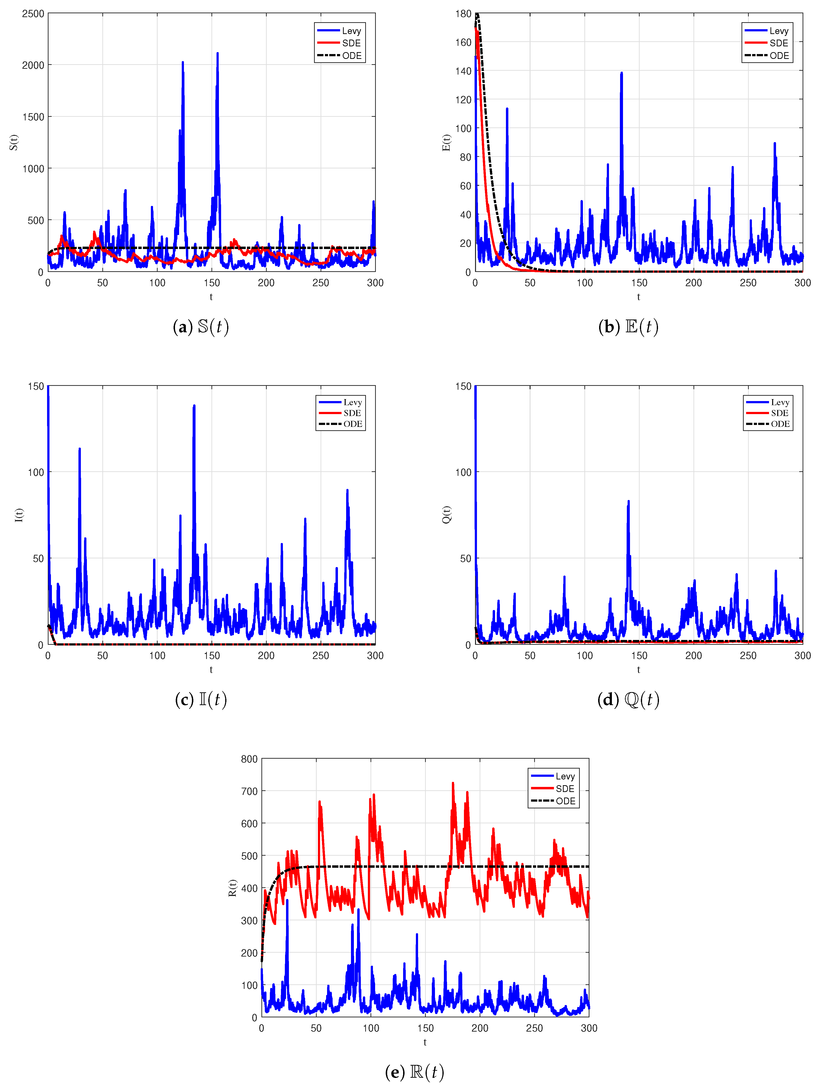
6.2. Numerical Simulation of Extinction

The simulations serve to validate the theoretical analysis of the model (1) and (3) and to confirm the results of Theorem 2. We assume a step size of $\Delta t=0.10$ and an initial value of the parameters value for model (3) taking from

Table 2. Model parameters with two different sets of values for numerical simulation.

Parameter	Set 1	Set 2
$S\left(0\right)$	500	1000
$E\left(0\right)$	20	50
$I\left(0\right)$	10	30
$Q\left(0\right)$	5	15
$R\left(0\right)$	0	5
b	0.02	0.03
$\beta$	0.5	0.7
$\delta$	0.1	0.15
$\mu$	0.01	0.02
$d_1$	0.05	0.07
$d_2$	0.03	0.05
$d_3$	0.02	0.03
$\eta$	0.01	0.02
$\lambda$	0.2	0.25
$ϵ$	0.03	0.04
$\gamma$	0.1	0.15
$\tau$	0.08	0.1
$N\left(0\right)$	535	1100

(Set 1) where $h_1=0.02,h_2=0.06,h_3=0.004,h_4=0.04$. To validate the result of Theorem 2 the threshold value denoted as ${\mathbf{R}}_{\mathbf{0}}^{\mathit{E}}$, is smaller than 1. According to Theorem 2, the disease will eventually disappear entirely from the human population. The limit of t is 0 since t approaches infinity. There is no limit other than zero as t approaches infinity. You may see the findings visually in Figure 1. The efficacy of COVID-19 therapy can differ across patients and may fluctuate over time for the same individual. To address this variability, Lévy noise may be included into the model. Lévy noise denotes random fluctuations or unpredictability within a stochastic system, perhaps originating from several reasons. Increasing the level of white noise in such models can have interesting consequences on system dynamics, including accelerating the elimination of COVID-19 viruses. External variables that introduce fluctuations or unpredictability into the environment may cause an increase in Lévy noise, influencing disease behavior and treatment response.

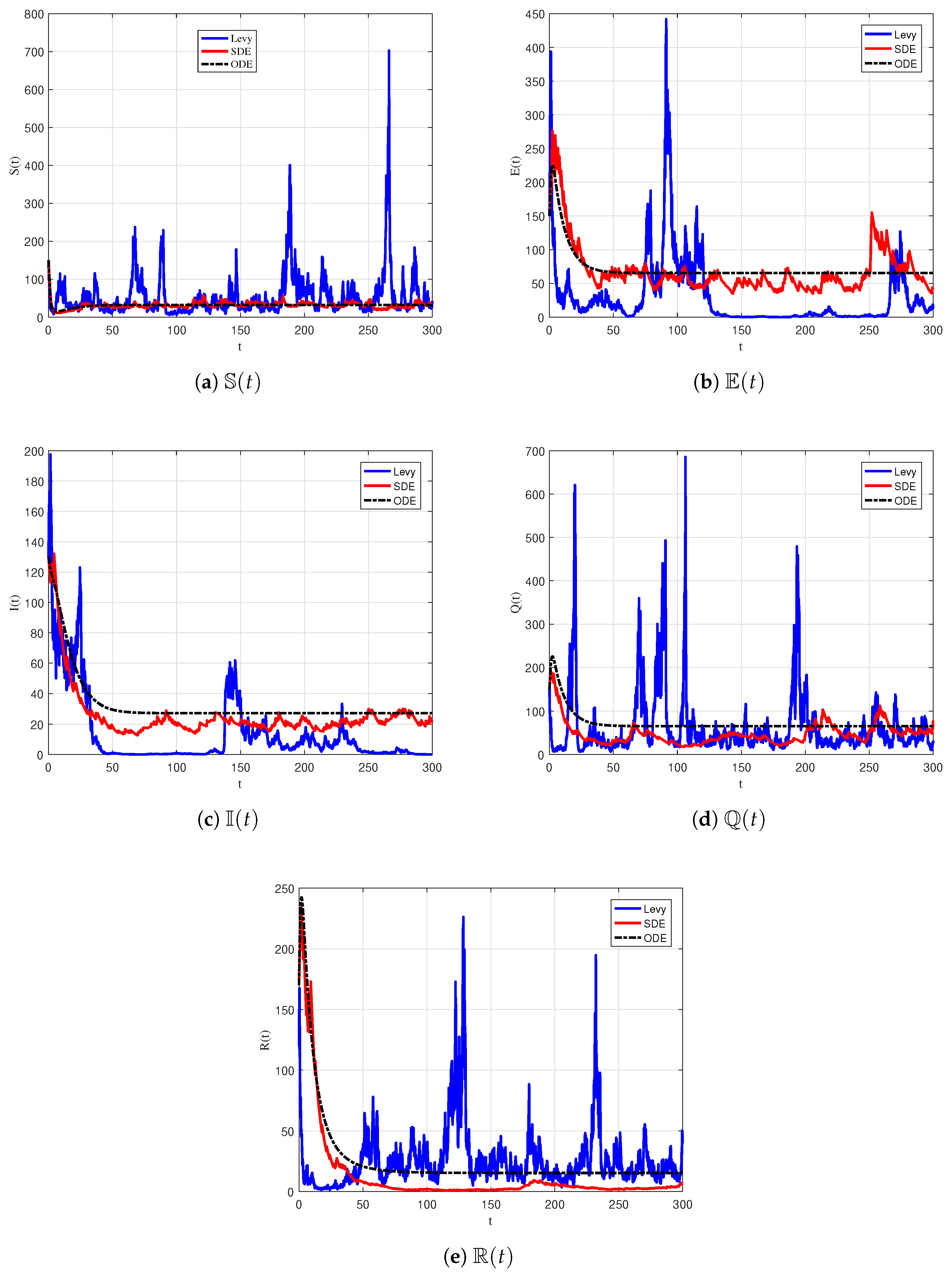
6.3. Numerical Simulation of Persistence

To validate the results of Theorem 3, then we select the parameters value for model (3) and the initial value taken from Table 2 (Set 2), where $h_1=0.02,h_2=0.03,h_3=0.004,h_4=0.05$. Based on the provided data, it is confirmed that ${\mathbf{R}}_{\mathbf{0}}^{\mathit{P}}>1$ and the reproduction number ${\mathbf{R}}_{\mathbf{0}}^{\mathit{P}}=1.9>1$. Thus, based on Theorem 3, the infectious disease described by the model (3) will continue to be in the society until the requirements mentioned above are met (see Figure 2). The model demonstrates a very low level of white noise intensities when ${\mathbf{R}}_{\mathbf{0}}^{\mathit{P}}>1$. Figure 2a–e and Figure 3a–e illustrate that the trajectories of the model reach the respective constant solutions, signifying stochastic asymptotic stability. Moreover, when the amplitude of white noise increases with time, the findings outlined in Theorem 3 are readily verified. Figure 2 demonstrates that an increase in white noise intensity results in the growth of viral cells. As a result, COVID-19 cells remain in the body without reduction, finally achieving a stable dynamic pattern.

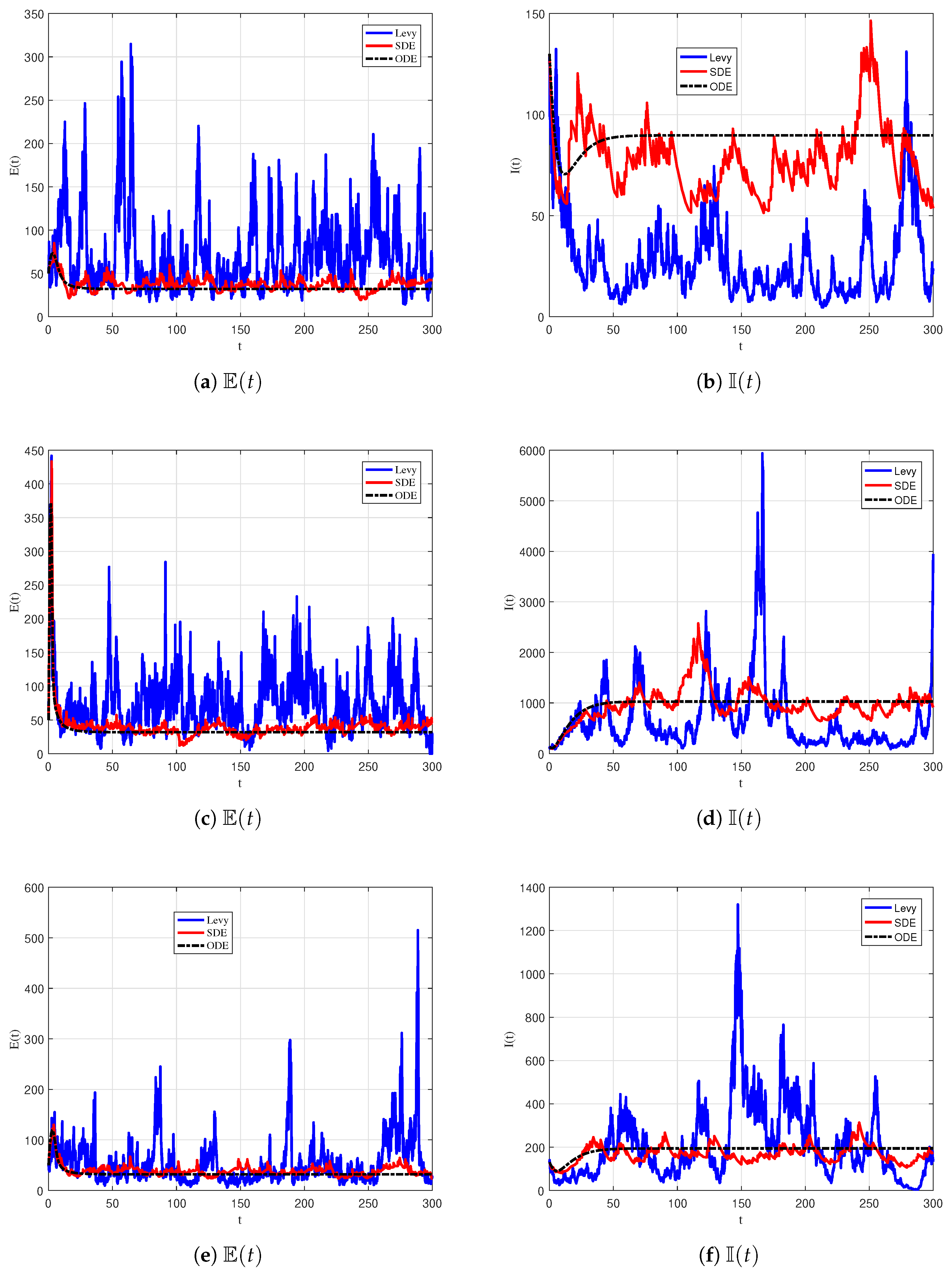
6.4. Effects of Lévy Noise

In the latter two portions of this section, we examined the dynamical behavior of the proposed system using numerical simulations, predominantly affected by variations in the values of the threshold ${\mathbf{R}}_{\mathbf{0}}^{\mathit{P}}$. We will now focus on examining the long-term subjective components of the system. Model (3) includes two types of noise to enhance its authenticity. To substantiate this claim, it is crucial to examine the impact of Lévy noise and white noise on the dynamics of the model (3). To do this, we have selected the different values of ${\delta }_1,{\delta }_2,{\delta }_3,{\delta }_4,{\delta }_5$ to be appropriately large while leaving the remaining values taken from Table 2 (Set 2). To do this, we have different values of $h_1=0.2,h_2=0.75,h_3=0.44,h_4=0.33$ to be appropriately large. This indicates that model (3) exhibits the complete elimination of the disease in the population, whereas the comparable deterministic model shows a persistent epidemic. Furthermore, Figure 3 depicts a visual representation of the paths leading to the answer. This indicates that augmenting the values of ${\delta }_1,{\delta }_2,{\delta }_3,{\delta }_4,{\delta }_5$ leads to stochastic trajectories characterized by considerable fluctuations and sudden leaps, as seen in Figure 3a–f.

7. Conclusions

The recent epidemic of COVID-19 continues to be one of the most serious diseases globally, and as of yet, no conclusive cure has been determined. It is essential to recognize that most real-world occurrences of infectious diseases are not entirely predictable but rather display intrinsic randomness. Employing stochastic theory, we constructed a mathematical model for COVID-19 that incorporates the disease’s characteristics, allowing us to examine its transmission patterns within a variable population context. Utilizing stochastic Lyapunov function theory, we established the existence of solutions alongside their positivity. Additionally, we analyzed the extinction and stationary distribution of the illness, determining the criteria necessary for eradicating COVID-19. Our findings underscore the substantial influence of the noise level on the transmission dynamics of COVID-19. The extinction of COVID-19-infected individuals is seen to rise with increasing noise strengths, although the durability of the infection diminishes. All aforementioned analytical conclusions are graphically supported by numerical simulations. This study shows that stochastic analysis offers a superior framework for exhibiting the dynamic behavior of epidemic infections, including the new COVID-19, since it considers multiple time- and location-dependent aspects related to the disease.

In future studies, this system can be extended by including the latent class to more effectively characterize disease progression. The model may also be fractionalized utilizing operators like Atangana–Baleanu, Caputo, or Caputo–Fabrizio to investigate the memory effects in disease dynamics. Moreover, researchers can employ optimal control methods to reduce the infected population by choosing appropriate control variables, hence improving the efficacy of intervention measures.

References

1. Lai, C.-C.; Shih, T.-P.; Ko, W.-C.; Tang, H.-T.; Hsueh, P.-R. Severe acute respiratory syndrome coronavirus 2 (SARS-CoV-2) and corona virus disease-2019 (COVID-19): The epidemic and the challenges. Int. J. Antimicrob. Agents 2020, 55, 105924. [Google Scholar] [CrossRef]
2. De Groot, R.J.; Baker, S.C.; Baric, R.S.; Brown, C.S.; Drosten, C.; Enjuanes, L.; Fouchier, R.A.M.; Galiano, M.; Gorbalenya, A.E.; Memish, Z.A.; et al. Commentary: Middle East respiratory syndrome coronavirus (MERS-CoV): Announcement of the Coronavirus Study Group. J. Virol. 2013, 87, 7790–7792. [Google Scholar] [CrossRef]
3. WHO MERS-CoV Research Group. State of knowledge and data gaps of Middle East respiratory syndrome coronavirus (MERS-CoV) in humans. PLoS Curr. 2013, 5, 1–30. [Google Scholar] [CrossRef]
4. Chikungunya, E.C.D.C. Factsheet for Health Professionals. Available online: http://ecdc.europa.eu/en/ (accessed on 1 April 2025).
5. World Health Organization. Coronavirus Disease 2019 (COVID-19): Situation Report, 67; World Health Organization: Geneva, Switzerland, 2020. [Google Scholar]
6. World Health Organization. Coronavirus Disease 2019 (COVID-19): Situation Report, 85; World Health Organization: Geneva, Switzerland, 2020. [Google Scholar]
7. Cao, Z.; Zhu, J.; Wang, Z.; Peng, Y.; Zeng, L. Comprehensive pan-cancer analysis reveals ENC1 as a promising prognostic biomarker for tumor microenvironment and therapeutic responses. Sci. Rep. 2024, 14, 25331. [Google Scholar] [CrossRef]
8. Perko, L. Differential Equations and Dynamical Systems; Springer Science & Business Media: Berlin/Heidelberg, Germany, 2013; Volume 7. [Google Scholar]
9. Arnold, L. Stochastic Differential Equations; Wiley: Hoboken, NJ, USA, 1974. [Google Scholar]
10. Wu, Z.; McGoogan, J.M. Characteristics of and important lessons from the coronavirus disease 2019 (COVID-19) outbreak in China: Summary of a report of 72 314 cases from the Chinese Center for Disease Control and Prevention. JAMA 2020, 323, 1239–1242. [Google Scholar] [CrossRef] [PubMed]
11. Sinan, M.; Alharthi, N.H. Mathematical analysis of fractal-fractional mathematical model of COVID-19. Fractal Fract. 2023, 7, 358. [Google Scholar] [CrossRef]
12. Khader, M.M.; Adel, M. Modeling and numerical simulation for covering the fractional COVID-19 model using spectral collocation-optimization algorithm. Fractal Fract. 2022, 6, 363. [Google Scholar] [CrossRef]
13. Gray, A.; Greenhalgh, D.; Hu, L.; Mao, X.; Pan, J. A stochastic differential equation SIS epidemic model. SIAM J. Appl. Math. 2011, 71, 876–902. [Google Scholar] [CrossRef]
14. Zhou, Y.; Zhang, W.; Yuan, S. Survival and stationary distribution of a SIR epidemic model with stochastic perturbations. Appl. Math. Comput. 2014, 244, 118–131. [Google Scholar] [CrossRef]
15. Lu, Q. Stability of SIRS system with random perturbations. Phys. A Stat. Mech. Its Appl. 2009, 388, 3677–3686. [Google Scholar] [CrossRef]
16. Ji, C.; Jiang, D. Threshold behaviour of a stochastic SIR model. Appl. Math. Model. 2014, 38, 5067–5079. [Google Scholar] [CrossRef]
17. Din, A.; Ain, Q.T. Stochastic optimal control analysis of a mathematical model: Theory and application to non-singular kernels. Fractal Fract. 2022, 6, 279. [Google Scholar] [CrossRef]
18. An, X.; Du, L.; Jiang, F.; Zhang, Y.; Deng, Z.; Kurths, J. A few-shot identification method for stochastic dynamical systems based on residual multipeaks adaptive sampling. Chaos Interdiscip. J. Nonlinear Sci. 2024, 34, 073118. [Google Scholar] [CrossRef]
19. Ikram, R.; Hussain, G.; Khan, I.; Khan, A.; Zaman, G.; Raezah, A.A. Stationary distribution of stochastic COVID-19 epidemic model with control strategies. AIMS Math. 2024, 9, 30413–30442. [Google Scholar] [CrossRef]
20. Shah, S.M.A.; Nie, Y.; Alkhazzan, A.; Tunç, C. A stochastic hepatitis B model with media coverage and Lévy noise. J. Taibah Univ. Sci. 2024, 18, 2414523. [Google Scholar] [CrossRef]
21. Din, A.; Li, Y. Lévy noise impact on a stochastic hepatitis B epidemic model under real statistical data and its fractal–fractional Atangana–Baleanu order model. Phys. Scr. 2021, 96, 124008. [Google Scholar] [CrossRef]
22. Luzyanina, T.; Bocharov, G. Stochastic modeling of the impact of random forcing on persistent hepatitis B virus infection. Math. Comp. Simul. 2014, 96, 54–65. [Google Scholar] [CrossRef]
23. El Fatini, M.; Sekkak, I. Lévy noise impact on a stochastic delayed epidemic model with Crowly–Martin incidence and crowding effect. Phys. A Stat. Mech. Its Appl. 2020, 541, 123315. [Google Scholar] [CrossRef]
24. Zhu, Y.; Wang, L.; Qiu, Z. Dynamics of a stochastic cholera epidemic model with Lévy process. Phys. A 2022, 595, 127069. [Google Scholar] [CrossRef]
25. Zahri, M. Multidimensional Milstein scheme for solving a stochastic model for prebiotic evolution. J. Taibah Univ. Sci. 2014, 8, 186–198. [Google Scholar] [CrossRef]
26. Leng, X.N.; Feng, T.; Meng, X.Z. Stochastic inequalities and applications to dynamics analysis of a novel SIVS epidemic model with jumps. J. Inequal. Appl. 2017, 138. [Google Scholar] [CrossRef] [PubMed]
27. Danane, J.; Allali, K.; Hammouch, Z.; Nisar, K.S. Mathematical analysis and simulation of a stochastic COVID-19 Lévy jump model with isolation strategy. Results Phys. 2021, 23, 103994. [Google Scholar] [CrossRef] [PubMed]
28. Mao, X.; Wei, F.; Wiriyakraikul, T. Positivity preserving truncated Euler–Maruyama method for stochastic Lotka-Volterra competition model. J. Comput. Appl. Math. 2021, 394, 113566. [Google Scholar] [CrossRef]
Figure 1. Solution paths of the various compartments of model (3).
Fractalfract 09 00306 g001
Figure 2. The solution paths of the various compartments of model (3).
Fractalfract 09 00306 g002
Figure 3. The Lévy noise effects of the solution trajectories of E ( t ) and I ( t ) .
Fractalfract 09 00306 g003