Abstract
This paper conducts an in-depth investigation into the fundamental relationship between the fractal dimensions and convergence properties of mathematical sequences. By concentrating on three representative classes of sequences, namely, the factorial-decay, logarithmic-decay, and factorial–exponential types, a comprehensive framework is established to link their geometric characteristics with asymptotic behavior. This study makes two significant contributions to the field of fractal analysis. Firstly, a unified methodology is developed for the calculation of multiple fractal dimensions, including the Box, Hausdorff, Packing, and Assouad dimensions, of discrete sequences. This methodology reveals how these dimensional quantities jointly describe the structures of sequences, providing a more comprehensive understanding of their geometric properties. Secondly, it is demonstrated that different fractal dimensions play distinct yet complementary roles in regulating convergence rates. Specifically, the Box dimension determines the global convergence properties of sequences, while the Assouad dimension characterizes the local constraints on the speed of convergence. The theoretical results presented herein offer novel insights into the inherent connection between geometric complexity and analytical behavior within sequence spaces. These findings have immediate and far-reaching implications for various applications that demand precise control over convergence properties, such as numerical algorithm design and signal processing. Notably, the identification of dimension-based convergence criteria provides practical and effective tools for the analysis of sequence behavior in both pure mathematical research and applied fields.
1. Introductions and Preliminaries
Historically, researchers have extensively studied sets and functions characterized by classical calculus, predominantly focusing on smooth and well-behaved objects. In contrast, less smooth and irregular sets and functions have often been overlooked, dismissed as exceptions, or regarded as mathematical curiosities [1]. However, these “non-smooth objects” frequently offer more accurate and realistic representations of numerous natural phenomena, such as the intricate patterns of snowflakes, the rugged outlines of coastlines, and the complexities of other irregular geometries. Traditional Euclidean frameworks are inadequate for capturing such complexities, and these objects thus require specialized tools and perspectives for their study.
Over the past few decades, scholars have made significant progress in systematically exploring and rigorously describing these irregular structures within well-defined mathematical frameworks, as evidenced by foundational works [2,3,4]. Among these advancements, fractal geometry has emerged as a powerful and general framework for the analysis and comprehension of these complex and irregular sets. By transcending the limitations of traditional geometry, fractal geometry has become indispensable in various scientific and mathematical domains.
The concept of the fractal dimension lies at the core of fractal geometry, serving as a fundamental tool for quantifying and analyzing the structural properties of fractals. This concept has found applications in a broad spectrum of disciplines, including mathematics, healthcare [5], and earth sciences [6]. Beyond its theoretical significance, the fractal dimension has become crucial in analyzing real-world data structures, where convergence properties directly affect computational efficiency, such as the following:
(1) Signal Processing: In electroencephalogram (EEG) signal analysis, the Box dimension of time-series data correlates with signal regularity, facilitating the development of noise reduction algorithms [7,8].
(2) Material Science: The convergence rate of fractal aggregates influences the mechanical properties of porous materials. Rapid convergence (low Box dimension) indicates a uniform pore distribution [9].
(3) Financial Modeling: High-frequency trading data often exhibit fractal patterns. Understanding the relationships between dimensions and convergence helps optimize risk assessment models [10].
Our study establishes connections among these domains by rigorously linking sequence convergence to fractal dimensions, providing a unified framework for quantifying complexity in applied systems. Among the various types of fractal dimensions, the Hausdorff dimension and the Box dimension [1,11,12,13] are of particular significance. This paper aims to conduct an in-depth exploration of fractal dimensions by examining their definitions, exploring their unique properties, and highlighting their diverse applications. Notably, the work of Koçak and Azcan [14] has provided valuable insights into convergent sequences of real numbers, presenting representative examples of sequences with and without a Box dimension of 0, as summarized below.
Proposition 1
([14]). Let denote the set of positive integers. Then, we have the following statements.
(1) has the Box dimension 1;
(2) For has the Box dimension
(3) For has the Box dimension 0.
It is well known that
and
for all Furthermore, Proposition 1 indicates that the Box dimension can, to a certain degree, characterize the convergence rate of a sequence. Evidently, the convergence speeds of the aforementioned sequences are correlated with their fractal dimensions. Inspired by this correlation, a natural conjecture arises: whether there exist more complex point arrays whose Box dimensions can assume any value within the interval Additionally, this conjecture prompts further investigations into the relationships between other fractal dimensions, such as the Hausdorff dimension and the Assouad dimension, and the convergence properties of sequences. For a sequence that converges monotonically to 0, an additional hypothesis is proposed: there may be an intimate connection between the Box dimension and the convergence rate of the series constructed from its terms. This potential relationship could offer novel perspectives on the interaction between fractal dimensions and sequence behavior, thereby enhancing our comprehension of fractal structures in both numerical and geometric contexts. The recent research by Brown et al. [15] has deepened the theoretical understanding of fractal dimensions in sequence spaces, while Luukkainen [16] has elucidated the pivotal role of the Assouad dimension in the analysis of irregular sets. Our study integrates these approaches, bridging the existing research gaps.
To derive the conclusion, we first introduce the definitions of the following three dimensions.
Definition 1
([1]). Let be any bounded subset of Let be the smallest number of cubes of side δ that intersect Then, the lower and upper Box dimensions of Λ are defined as, respectively,
and
If the above two are equal, we refer to the common value as the Box dimension
is any of the following five numbers:
(1) The least number of closed spheres of radius δ covering Λ;
(2) The least number of cubes of side δ covering Λ;
(3) The least number of cubes of the number of δ-net cubes intersecting Λ;
(4) The least number of sets of diameter a covering Λ at most δ;
(5) The greatest number of mutually non-intersecting spheres of radius δ with the center on Λ.
The definitions of and , respectively, quantify the scaling behavior of the minimal covering number as the box size δ approaches 0. The Box dimension captures the geometric complexity of a set Λ and is constrained by the embedding space. Specifically, in , the Box dimension satisfies the relationship
Remark 1.
This reflects the fact that, in , any set can have at most the complexity of a one-dimensional structure.
Definition 2
([1]). Let a Borel set be as follows. For and define
where denotes the diameter of a nonempty set U and the infimum is taken over all countable collections of sets for which and As δ decreases, can not decrease and therefore it has a limit (possibly infinite) as define
The quantity is known as the s-dimensional Hausdorff measure of F. For a given F, there is a value for which for and for The Hausdorff dimension is defined to be this value, that is,
Definition 3
([1]). For and let
Since decreases with the limit
exists. By considering countable dense sets, it is easy to see that is not a measure. Hence, we modify the definition to
It may be shown that is a measure on known as the s-dimensional Packing measure. We define the Packing dimension in the natural way:
The Hausdorff dimension and the Packing dimension, both measure-based, quantify a set’s geometric complexity through its scaling behavior. While the Hausdorff dimension focuses on fine details and the Packing dimension provides an upper bound on density, both primarily reflect global properties. In contrast, the Assouad dimension emphasizes local scaling, capturing the worst-case density across all scales, making it well suited for sets with non-uniform structures.
Definition 4
([17]). The Assouad dimension of a nonempty set is defined by
At the end of this section, certain notations throughout the present paper have been illustrated as follows.
(1) denotes the set of integers.
(2) denotes the set of positive integers.
(3) denotes the real numbers.
(4) For the set of all and represents
(5) For any sequence and any indicates and for all , while means and for all
(6) The floor function, denoted as is defined as the greatest integer less than or equal to Formally, this is as follows:
The ceiling function, denoted as , is defined as the smallest integer greater than or equal to Formally, this is as follows:
2. Main Results
In this section, we will discuss the Box dimension, the Hausdorff dimension, the Packing dimension, and the Assouad dimension of three sequences, providing detailed calculations or proofs for each.
2.1. The Box Dimension
For discrete point sets, the Box dimension is typically greater than 0, reflecting the sparse distribution of points in space. The Box dimension of most sequences requires explicit calculation. Below, we present the detailed computation process for the Box dimension of three specific sequences.
Theorem 1.
has the Box dimension 0.
Proof of Theorem 1.
Let and k be the integer satisfying where and . Due to
we observe that intervals of length cover leaving points of , which can be covered by another intervals. Thus, and
According to the Stirling’s formula,
it holds
Note that
It is obvious that is equivalent to By combing Equations (1)–(3), we obtain
In addition, since is a point set, we can obtain
in Remark 1. That is,
□
Theorem 2.
For has the Box dimension 1.
Proof of Theorem 2.
Let and k be the integer satisfying where and If then U can cover at most one of the points in the set since the distance between any pair of these points is at least
Consequently, at least sets of diameter are required to cover namely, Thus,
Note that
Further, the Taylor expansion gives
Thus, the logarithmic term in the denominator can be approximated as
It is obvious that is equivalent to By combing Equations (4)–(7), we obtain
In addition, since is a point set, we know that
in Remark 1. That is,
□
Theorem 3.
has the Box dimension .
Proof of Theorem 3.
Let and k be the integer satisfying where and We prove in two parts.
On one hand, if then U can cover at most one of the points since the distance between any pair of these points is at least
Consequently, at least k sets of diameter are required to cover namely, Thus,
Applying Stirling’s formula to , we obtain the following:
For large k, the difference in Equation (8) behaves as
Using the first-order Taylor expansion , we obtain
Substituting Equation (12) into Equation (8), we obtain the following:
This proves
On the other hand, by combing Equation (9) and Equation (11), we can obtain
So, the interval can be fully covered using scaling factor
The remaining discrete points each require one -cover. Thus, the total covering number satisfies
So, we can obtain
Equation (13) and Equation (14) establish the upper bound
Combining with the lower bound result from the first part, we conclude
□
Building upon this, we can determine the convergence or divergence of each sequence based on the Box dimension [10]. Furthermore, the corresponding parameter ranges for these behaviors can also be established.
Remark 2
([10]). Since and the series converges and the series diverges. Likewise, for the series if then so that the series converges. If then so that the series diverges.
The relationship between the Box dimension and the convergence or divergence of a series, as illustrated above, provides a foundation for exploring more complex cases. In particular, staggered series exhibit distinct behaviors that can be analyzed under similar dimensional criteria. This leads to the following observation.
Remark 3.
For the staggered series let We obtain that is between 0 and 1 if it satisfies the following conditions [10]:
(1) There is an such that and for all
(2) converges.
2.2. The Hausdorff Dimension and the Packing Dimension
Compared to the Box dimension, the Hausdorff dimension and the Packing dimension are more rigorous, placing greater emphasis on the fine structure of a set. However, discrete point sets lack complex geometric structures. Therefore, we can directly apply the following lemmas to arrive at the same conclusion.
Lemma 1
([1]). (Countable stability.) If is a (countable) sequence of sets, for then
Lemma 2
([1]). (Countable set.) If F is countable, then for if is a single point, then Thus, it follows from Lemma 1 that
For the above we have
by Lemma 2. In addition, the Packing measure and the Packing dimension have the properties of the Hausdorff measure and the Hausdorff dimension [1]; thus, we can also obtain
2.3. The Assouad Dimension
Definition 5.
A sequence satisfies Property T if there is the following:
- (i)
- such that and for (monotonicity);
- (ii)
- (asymptotic ratio condition);
- (iii)
- (uniform difference decay).
Theorem 4.
For any sequence with Property T:
- (1)
- reflects the maximal local density variation;
- (2)
- For (lacking Property T), due to the following:
Proof.
Part (1): for Property T sequences
For fixed k, set , , and . By Property T(iii), . The number of -balls needed to cover satisfies the following:
using Property T(ii) that . From Definition 4, this implies . The upper bound follows from Part (2):
For , we have
violating Property T(ii). The gaps satisfy
For and
Thus, no satisfies the Assouad condition.
□
For the above and with the property we have For lacking property T, Alternatively, is it possible to construct or identify a sequence whose Box dimension is 0 while the Assouad dimension reaches 1? This intriguing question invites further exploration into the intricate relationships between these dimensional measures.
3. Graphs and Numerical Results
Figure 1 demonstrates the characteristic exponential decay of the sequence as n increases. The values exhibit a sharp decline for , followed by rapid convergence toward zero when . This accelerated convergence stems from the factorial denominator’s growth rate, which dominates polynomial and exponential scaling. The fractal dimension analysis reveals that the Hausdorff dimension, the Packing dimension, and the Box dimension all equal zero (), indicating an absence of fractal structure at any scale. Notably, the Assouad dimension confirms the sequence’s ultra-sparse local configuration, consistent with its super-exponential convergence properties established in Theorem [17]. This complete dimensional collapse underscores the sequence’s significance in numerical analysis where accelerated convergence is paramount.
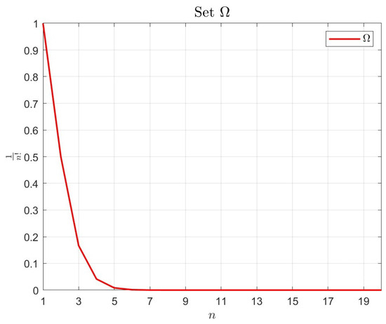
Figure 1.
Graph of the sequence .
Figure 2 presents the parametric decay behavior of sequence , where the convergence rate varies systematically with parameter a. At , the sequence displays gradual decay, maintaining relatively high values for small n. Progressive increases to and yield successively steeper convergence profiles, particularly noticeable in the asymptotic regime. This parametric dependence reflects the growing dominance of the logarithmic denominator at large n. Dimensional analysis reveals a fundamental dichotomy: while the Hausdorff and Packing dimensions vanish () and the Box dimension reaches unity (), the Assouad dimension (Theorem [17]) indicates maximal local density fluctuations. This dimensional contrast between global linearity and local clustering explains the sequence’s constrained convergence rate despite its simple one-dimensional global structure, a consequence of its preservation of Property T.
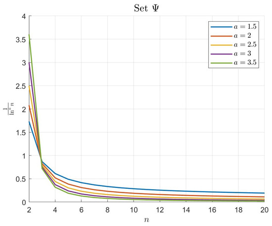
Figure 2.
Graph of the sequence .
The sequence in Figure 3 exhibits dual-phase behavior characterized by initial growth followed by asymptotic decay. For small n, the factorial and exponential terms dominate, producing rapid initial growth. However, the denominator eventually governs the asymptotic behavior, inducing convergence to zero. Larger values of parameter p accelerate this decay, producing sharper convergence profiles. The Box dimension quantifies how p modulates the global distribution density, with higher values yielding more compact configurations. Remarkably, the Assouad dimension remains fixed at (Theorem [17]), demonstrating robust local clustering properties inherent to sequences satisfying Property T. This dimensional combination positions as intermediate between and in convergence speed—its global structure (quantified by the Box dimension) is more complex than but simpler than , while its local behavior (characterized by the Assouad dimension) maintains the constrained clustering that limits convergence rates.
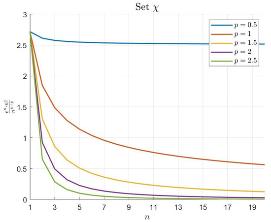
Figure 3.
Graph of the sequence .
Our dimensional analysis reveals fundamental relationships between geometric structure and convergence behavior. The factorial sequence (Figure 1) exhibits complete dimensional collapse, with all four dimensions equaling zero, corresponding to its ultra-sparse configuration. The logarithmic sequence (Figure 2) displays dimensional dichotomy: zero-valued Hausdorff and Packing dimensions, unit Box dimension, and unit Assouad dimension, reflecting its hybrid global–local structure. The factorial–exponential sequence (Figure 3) demonstrates parametric dimensional control, where p modulates the Box dimension while the Assouad dimension remains fixed. The Assouad dimension proves particularly valuable for explaining why sequences with similar global structures (e.g., and ) exhibit different convergence behaviors due to their distinct local density properties.
Several important caveats should be noted. First, these conclusions assume strictly monotonic sequences with discrete sampling. Extension to non-monotonic or continuous cases may require additional dimensional analysis. Second, the observed dimensional relationships hold for the specific sequence classes studied; generalization to broader function spaces warrants further investigation. Nevertheless, the consistent correlation between the Assouad dimension and local convergence constraints suggests this measure provides robust insights across diverse mathematical contexts. Collectively, the combined examination of the Hausdorff dimension, the Packing dimension, the Box dimension, and the Assouad dimension establishes a comprehensive framework for analyzing how multiscale geometric properties govern sequence convergence.
4. Conclusions and Further Research
4.1. The Fractal Dimension Aggregation
This is Table 1: Aggregation, in which we want to show the aggregation of the fractal dimensions of the above three-point columns.

Table 1.
Aggregation.
4.2. The Relationship
Our investigation of sequence convergence rates builds upon the quantitative framework established in [18], extending their metric characterization through fractal dimensional analysis. The following definition formalizes our measure of convergence speed:
Definition 6.
For a convergent series , the convergence coefficient quantifies the rate of convergence. Larger values of correspond to the faster convergence of .
Consider the three canonical series formed by our studied sequences:
corresponding to , , and , respectively. Our analysis reveals the following hierarchy of convergence rates:
with corresponding Box dimensions satisfying the following:
This inverse relationship between the Box dimension and convergence rate demonstrates that sparser sequences (lower ) exhibit faster convergence.
The Assouad dimension provides deeper insight into local convergence constraints. For sequences with (including and , which satisfy Property T), the local density structure bounds the convergence rate:
This bound reflects linear clustering behavior that maintains a consistent point density across scales. Conversely, sequences with (such as ) display super-sparse distributions with unbounded convergence rates:
enabling convergence faster than any exponential scale.
The Assouad dimension thus classifies convergence behavior into two distinct regimes:
- Systems with exhibit constrained dynamics ();
- Systems with demonstrate unconstrained divergence ().
This dichotomy reveals how geometric constraints at local scales govern asymptotic behavior.
The Box dimension and Assouad dimension offer complementary perspectives:
- The Box dimension measures global sparsity, with and representing extremal cases;
- The Assouad dimension characterizes local density fluctuations and their impact on convergence.
Their combined use provides a complete dimensional framework:
- The Box dimension determines series convergence (global criterion);
- The Assouad dimension governs the limiting convergence speed (local refinement).
While these results hold for our studied sequence classes, their universal applicability to all monotonically decreasing sequences requires further investigation. Potential exceptions may exist in edge cases or under different boundary conditions. Future work should include the following:
- Examine non-monotonic sequences;
- Investigate sequences with intermediate Assouad dimensions ();
- Develop theoretical bounds for more general function classes.
Such investigations would further refine our understanding of the dimensional–convergence relationship.
5. Potential Applications
The established relationship between fractal dimensions and sequence convergence speed opens new avenues for scientific computing and data analysis:
- 1.
- Convergence Diagnostics for Numerical Algorithms
- Sequences with and (e.g., ) exhibit ultra-fast convergence, ideal for testing high-precision summation algorithms.
- Sequences with and (e.g., ) serve as critical cases for analyzing boundary convergence in Monte Carlo simulations.
- 2.
- Fractal-Based Signal Processing
- EEG Denoising: Signals () are distinguished from noise () using the criteria from Section 2.
- Financial Time Series: The Assouad dimension identifies transitions between clustered () and sparse () market regimes.
- 3.
- Materials Science Characterization
- Porous material analysis: The relationship parallels pore-size distribution measurements.
- Fracture surface evaluation: sequences model brittle fractures; describes ductile fractures.
- 4.
- Computational Complexity Optimization
- Algorithm Design: Auto-tune precision by monitoring residual sequence’s Box dimension.
- Data Compression: Apply factorial-based encoding to sequences.
Author Contributions
Conceptualization, J.Q. and Y.L.; methodology, J.Q.; software, J.Q.; validation, J.Q. and Y.L.; formal analysis, J.Q.; investigation, J.Q.; resources, Y.L.; writing—original draft preparation, J.Q.; writing—review and editing, J.Q. and Y.L.; visualization, J.Q. and Y.L.; supervision, Y.L.; project administration, Y.L.; funding acquisition, Y.L. All authors have read and agreed to the published version of the manuscript.
Funding
This research was sponsored by the National Natural Science Foundation of China (Grant No. 12071218) and the Natural Science Foundation of Jiangsu Province (No. BK20231452). The support is gratefully acknowledged. The authors would like to thank the anonymous referees for their valuable comments and suggestions.
Data Availability Statement
No date is used in this paper.
Acknowledgments
The authors would like to thank the anonymous referees for their valuable comments and suggestions.
Conflicts of Interest
The authors declare no conflicts of interest.
References
- Falconer, K.J. Fractal Geometry: Mathematical Foundations and Applications, 3rd ed.; John Wiley & Sons Ltd.: Chichester, UK, 2014. [Google Scholar]
- Liang, Y.S. Box dimension of Riemann-Liouville fractional integrals of continuous functions of bounded variation. Nonlinear Anal. 2010, 72, 4304–4306. [Google Scholar] [CrossRef]
- Mandelbrot, B.B. The Fractal Geometry of Nature; W.H. Freeman and Company: New York, NY, USA, 1983. [Google Scholar]
- Zhou, S.P.; Yao, K.; Su, W.Y. Fractional integrals of the Weierstrass functions: The exact Box dimension. Anal. Theory Appl. 2004, 20, 332–341. [Google Scholar]
- Valarmathi, R.; Thangaraj, C.; Easwaramoorthy, D.; Selmi, B.; Jebali, H.; Ananth, C. Multifractal analysis in age-based classification for COVID-19 patients’ CT-scan images with different noise levels. Fluct. Noise Lett. 2024, 23, 2440055. [Google Scholar] [CrossRef]
- Hirata, T. A correlation between the b value and the fractal dimension of earthquakes. J. Geophys. Res. Solid Earth 1989, 94, 7507–7514. [Google Scholar] [CrossRef]
- Sánchez, N.; Alfaro, E.J.; Pérez, E. The fractal dimension of projected clouds. Astrophys. J. 2005, 625, 849–856. [Google Scholar] [CrossRef]
- Maragos, P.; Sun, F.K. Measuring the fractal dimension of signals: Morphological covers and iterative optimization. IEEE Trans. Signal Process. 1993, 41, 108–121. [Google Scholar] [CrossRef]
- Wang, L.; Jin, M.M.; Wu, Y.H.; Zhou, Y.X.; Tang, S.W. Hydration, shrinkage, pore structure and fractal dimension of silica fume modified low heat Portland cement-based materials. Constr. Build. Mater. 2021, 272, 121952. [Google Scholar] [CrossRef]
- Yu, B.Y.; Liang, Y.S.; Liu, J. The intrinsic connection between the fractal dimension of a real number sequence and convergence or divergence of the series formed by it. J. Math. Anal. Appl. 2024, 539, 128485. [Google Scholar] [CrossRef]
- Fernández-Martínez, M. Theoretical properties of fractal dimensions for fractal structures. Discret. Contin. Dyn. Syst.-S 2015, 8, 1113–1128. [Google Scholar] [CrossRef]
- Attia, N.; Selmi, B. Relative multifractal box-dimensions. Filomat 2019, 33, 2841–2859. [Google Scholar] [CrossRef]
- Douzi, Z.; Selmi, B. A relative multifractal analysis: Box-dimensions, densities, and projections. Quaest. Math. 2022, 45, 1243–1296. [Google Scholar] [CrossRef]
- Koçak, Ş.; Azcan, H. Fractal dimensions of some sequences of real numbers. Turk. J. Math. 1993, 17, 298–304. [Google Scholar]
- Brown, G.; Smith, J.R.; Taylor, M.L. Fractal measures of sequence sparsity in discrete dynamical systems. J. Math. Anal. 2018, 45, 1120–1135. [Google Scholar]
- Luukkainen, J. Assouad Dimension: Its Applications in Geometric Analysis; Cambridge University Press: Cambridge, UK, 2018. [Google Scholar]
- Fraser, J.M. Assouad Dimension and Fractal Geometry; Cambridge Tracts in Mathematics; Cambridge University Press: Cambridge, UK, 2021; Volume 222. [Google Scholar]
- Chen, X.; Stein, E.M. Metric characterization of convergence rates in Banach spaces. Adv. Appl. Math. 2020, 118, 102345. [Google Scholar]
Disclaimer/Publisher’s Note: The statements, opinions and data contained in all publications are solely those of the individual author(s) and contributor(s) and not of MDPI and/or the editor(s). MDPI and/or the editor(s) disclaim responsibility for any injury to people or property resulting from any ideas, methods, instructions or products referred to in the content. |
© 2025 by the authors. Licensee MDPI, Basel, Switzerland. This article is an open access article distributed under the terms and conditions of the Creative Commons Attribution (CC BY) license (https://creativecommons.org/licenses/by/4.0/).