Optical Solutions of the Nonlinear Kodama Equation with the M-Truncated Derivative via the Extended (G^′/G)-Expansion Method

Abstract

The main purpose of this article is to study the optical solutions of the nonlinear Kodama equation with the M-truncated derivative by using the extended $(G^{\prime }/G)$-expansion method. Firstly, the nonlinear Kodama equation with the M-truncated derivative is transformed into a nonlinear ordinary differential equation based on the principle of homogeneous equilibrium and the traveling wave transformation. Secondly, the optical solutions of the nonlinear Kodama equation with the M-truncated derivative are constructed by using the extended $(G^{\prime }/G)$-expansion method. Finally, three-dimensional, two-dimensional, and contour maps of partial solutions are obtained by using Matlab R2023b mathematical software.

1. Introduction

Complex fractional partial differential equations (CFPDEs) [1,2] are widely used in fields such as physics, chemistry, biology, geophysics, communication, and engineering. For example, in physics, CFPDEs are used to describe various physical phenomena with memory and diffusion processes. In the field of communications [3], CFPDEs can effectively reduce and enhance signals. In finance [4], CFPDEs are used to establish financial market models incorporating memory and volatility. In addition to the aforementioned fields, CFPDEs have broad application prospects in multiple areas. The most typical CFPDE is the well-known fractional-order Schrödinger equation [5,6]. In recent years, many fractional-order derivatives [7,8,9,10] have been proposed and combined with nonlinear partial differential equations to form fractional order partial differential equations. There are many types of fractional derivatives, such as the conformable fractional derivative [11], the Riemann–Liouville fractional derivative [12], and the M-truncated derivative [13,14]. The nonlinear Kodama equation with the M-truncated derivative (NLKE-MTD) is a very important class of CFPDE, which is usually described as follows [15]:

$$i{T}_{k,t}^{\alpha ,\beta }u+u_{xx}+i{u}_{xxx}+{\epsilon }_1{\left|u\right|}^{2}u+i{\epsilon }_2{\left|u\right|}^2{u}_x+i{\epsilon }_3{u}^2{u}_x=0,$$

(1)

where $u=u(x,t)$ stands for the complex function. $T_{k,t}^{\alpha ,\beta }(·)$ represents the M-truncated derivative, its definition and properties will be provided in Section 2. Parameters ${\epsilon }_1$, ${\epsilon }_2$, and ${\epsilon }_3$ are arbitrary constants. i represents the imaginary unit satisfying $i^2=-1$. In [15], Mohammed and his collaborators obtained soliton solutions of Equation (1) by using the generalized Riccati equation method and the Jacobi elliptic function method, respectively. In [16], Algolam et al. obtained the soliton solutions of the stochastic version of the nonlinear Kodama equation (NLKE) by using the $(G^{\prime }/G)$-expansion method and the mapping method, respectively.

The subsequent sections are arranged as follows: In Section 2, NLKE-MTD is transformed into a nonlinear ordinary differential equation. In Section 3, the optical solutions of NLKE-MTD are constructed by using the extended $(G^{\prime }/G)$-expansion method. In Section 4, three-dimensional, two-dimensional, and contour maps of two sets of solutions are obtained by using Matlab mathematical software. In Section 5, a brief conclusion is given.

2. Preliminary

2.1. The M-Truncated Fractional-Derivative and Its Properties

Definition 1

([17]). Let $f:[0,+\infty )\to (-\infty ,+\infty )$. For $0<\alpha \le 1$, the truncated M-fractional derivative is denoted as

$$T_{k,t}^{\alpha ,\beta }f(t)=\underset{h\to 0}{lim}{\displaystyle \frac{f(t{E}_{k,\beta }(h{t}^{1-\alpha }))-f(t)}{h}},\beta \in (0,+\infty ),$$

(2)

where the constant α stands for a fractional-order derivative. $E_{k,\beta }(t)$ is a truncated Mittag–Leffler function defined as follows [18]:

$$E_{k,\beta }(t)=\sum _{k=0}^j{\displaystyle \frac{t^k}{\mathrm{\Gamma }(\gamma k+1)}},t\in \mathbb{C},$$

(3)

where $\mathbb{C}$ represents the complex number.

Remark 1.

MTD has the following properties [19]:

1. 

$T_{k,t}^{\alpha ,\beta }(af+bg)=a{T}_{k,t}^{\alpha ,\beta }f+b{T}_{k,t}^{\alpha ,\beta }g$;

2. 

$T_{k,t}^{\alpha ,\beta }(f)(t)={\displaystyle \frac{t^{1-\beta }}{\mathrm{\Gamma }(\beta +1)}}{\displaystyle \frac{df}{dt}}$;

3. 

$T_{k,t}^{\alpha ,\beta }(fg)=f{T}_{k,t}^{\alpha ,\beta }g+g{T}_{k,t}^{\alpha ,\beta }f$;

4. 

$T_{k,t}^{\alpha ,\beta }(f\circ g)(t)=f^{\prime }(g(t))T_{k,t}^{\alpha ,\beta }g(t)$;

5. 

$T_{k,t}^{\alpha ,\beta }{t}^{\gamma }={\displaystyle \frac{\gamma }{\mathrm{\Gamma }(\beta +1)}}{t}^{\gamma -\alpha }$.

2.2. The Extended $(G^{\prime }/G)$-Expansion Method [20]

We assume that there is a complex partial differential equation with M-truncated fractional-derivatives

$$\mathbf{P}(t,x,T_{k,t}^{\alpha ,\beta }u,u_x,u_{xx},\cdots )=0,$$

(4)

where $u=u(x,t)$ is the unknown function. We then introduce the fractional-order traveling wave transformation

$$u(x,t)=\mathcal{U}(\xi )e^{i\eta },\xi ={\zeta }_{1}x+{\displaystyle \frac{\mathrm{\Gamma }(\beta +1){\zeta }_2}{\alpha }}{t}^{\alpha },\eta ={\mu }_{1}x+{\displaystyle \frac{\mathrm{\Gamma }(\beta +1){\mu }_2}{\alpha }}{t}^{\alpha },$$

(5)

${\zeta }_1$, ${\zeta }_2$, ${\mu }_1$, and ${\mu }_2$ are nonzero constants.

Plugging Equation (5) into Equation (4), we can obtain the following nonlinear ordinary differential equation:

$$\mathbf{Q}(\mathcal{U}(\xi ),{\displaystyle \frac{d\mathcal{U}(\xi )}{d\xi }},{\displaystyle \frac{d^2\mathcal{U}(\xi )}{d{\xi }^2}},{\displaystyle \frac{d^3\mathcal{U}(\xi )}{d{\xi }^3}},\cdots )=0.$$

(6)

Next, we assume that the approximate solution of Equation (6) is

$$\mathcal{U}(\xi )=\sum _{i=0}^N{a}_i{({\displaystyle \frac{G^{\prime }}{G}})}^i+\sum _{i=1}^N{b}_i{({\displaystyle \frac{G^{\prime }}{G}})}^{-i},$$

(7)

and $G=G(\xi )$ satisfies

$$G{G}^{″}={\chi }_{1}G{G}^{\prime }+{\chi }_2{(G^{\prime })}^2+{\chi }_3{G}^2,$$

(8)

where ${\chi }_1$, ${\chi }_2$, and ${\chi }_3$ are real numbers.

The N in Equation (7) can be balanced by the highest order derivative term and the highest order nonlinear term in Equation (6). By substituting Equations (7) and (8) into Equation (6), a polynomial about ${(G^{\prime }/G)}^i$($i=0,1,2,\cdots ,N$) and ${(G^{\prime }/G)}^{-i}$($i=1,2,\cdots ,N$) can be obtained. Let all coefficients of the polynomial be zero. By solving this system of equations, we can obtain the coefficients of Equation (6). The above are the main steps of the extended ($G^{\prime }/G$)-expansion method. The detailed steps can refer to the literature [20].

2.3. Traveling Wave Transformation

Firstly, a very important fractional order traveling wave transformation is presented:

$$\begin{array}{c}\hfill u(x,t)=\mathcal{U}(\xi )e^{i\eta },\xi ={\zeta }_{1}x+{\displaystyle \frac{\mathrm{\Gamma }(\beta +1){\zeta }_2}{\alpha }}{t}^{\alpha },\eta ={\mu }_{1}x++{\displaystyle \frac{\mathrm{\Gamma }(\beta +1){\mu }_2}{\alpha }}{t}^{\alpha }\end{array}$$

(9)

where $U(\xi )$ represents the unknown function. ${\zeta }_1$, ${\zeta }_2$, ${\mu }_1$, and ${\mu }_2$ are nonzero constants.

Plugging Equation (9) into Equation (1) and separating the real and imaginary parts, we can obtain

$$\begin{array}{cc}\hfill & \mathrm{Imaginary}\mathrm{part}:{\epsilon }_1{\zeta }_1^3{\mathcal{U}}^{\prime \prime \prime }+({\zeta }_2+2{\mu }_1{\zeta }_1-3{\epsilon }_1{\mu }_1^2{\zeta }_1){\mathcal{U}}^{\prime }+{\zeta }_1({\epsilon }_2+{\epsilon }_3){\mathcal{U}}^2{\mathcal{U}}^{\prime }=0,\hfill \\ \hfill & \mathrm{Real}\mathrm{part}:({\zeta }_1^2-3{\epsilon }_1{\mu }_1{\zeta }_1^2){\mathcal{U}}^{″}+({\epsilon }_1{\mu }_1^3-{\mu }_2-{\mu }_1^2)\mathcal{U}+({\epsilon }_1-{\epsilon }_2{\mu }_1+{\epsilon }_3{\mu }_1){\mathcal{U}}^3=0,\hfill \end{array}$$

(10)

where $\mathcal{U}=\mathcal{U}(\xi )$.

Integrating Equation (10) with respect to $\xi$ simultaneously once and assuming the integral constant is zero, the following can be obtained:

$${\epsilon }_1{\zeta }_1^3{\mathcal{U}}^{″}+({\zeta }_2+2{\mu }_1{\zeta }_1-3{\epsilon }_1{\mu }_1^2{\zeta }_1)\mathcal{U}+{\displaystyle \frac{{\zeta }_1({\epsilon }_2+{\epsilon }_3)}{3}}{\mathcal{U}}^3=0.$$

(11)

Then, Equation (11) is equivalent to the second equation of Equation (9) and must satisfy the following conditions:

$${\displaystyle \frac{{\zeta }_1^2-3{\epsilon }_1{\mu }_1{\zeta }_1^2}{{\epsilon }_1{\zeta }_1^3}}={\displaystyle \frac{{\epsilon }_1{\mu }_1^3-{\mu }_2-{\mu }_1^2}{{\zeta }_2+2{\mu }_1{\zeta }_1-3{\epsilon }_1{\mu }_1^2{\zeta }_1}}={\displaystyle \frac{3({\epsilon }_1-{\epsilon }_2{\mu }_1+{\epsilon }_3{\mu }_1)}{{\zeta }_1({\epsilon }_2+{\epsilon }_3)}}.$$

(12)

If the conditions of Equation (12) are satisfied, then Equation (11) can be rewritten as

$${\mathcal{U}}^{″}+{\aleph }_2{\mathcal{U}}^3+{\aleph }_1\mathcal{U}=0,$$

(13)

where ${\aleph }_2={\displaystyle \frac{{\epsilon }_2+{\epsilon }_3}{3{\epsilon }_1{\zeta }_1^2}}$ and ${\aleph }_1={\displaystyle \frac{{\zeta }_2+2{\mu }_1{\zeta }_1-3{\epsilon }_1{\mu }_1^2{\zeta }_1}{{\epsilon }_1{\zeta }_1^3}}$.

3. Optical Solutions of NLKE-MTD

Using the principle of homogeneous equilibrium, we can obtain $N=1$ by balancing the highest order derivative term ${\mathcal{U}}^{″}$ and the highest order nonlinear term ${\mathcal{U}}^3$. Then, Equation (7) can be expressed as

$$\mathcal{U}(\xi )=a_1({\displaystyle \frac{G^{\prime }}{G}})+a_0+b_1{({\displaystyle \frac{G^{\prime }}{G}})}^{-1}.$$

(14)

By using Equations (8) and (14), we can obtain

$$\begin{array}{cc}\hfill & {\mathcal{U}}^{″}(\xi )=2a_1({\chi }_2-1){({\displaystyle \frac{G^{\prime }}{G}})}^3+[2a_1{\chi }_1({\chi }_2-1)+a_1{\chi }_1({\chi }_2-1)]{({\displaystyle \frac{G^{\prime }}{G}})}^2\hfill \\ \hfill & +[a_1{\chi }_1^2+2a_1{\chi }_3({\chi }_2-1)]({\displaystyle \frac{G^{\prime }}{G}})+[a_1{\chi }_1{\chi }_3+b_1{\chi }_1({\chi }_2-1)]\hfill \\ \hfill & +[b_1{\chi }_1^2+2b_1{\chi }_3({\chi }_2-1)]{({\displaystyle \frac{G^{\prime }}{G}})}^{-1}+(b_1{\chi }_1^2+2b_1{\chi }_1{\chi }_3){({\displaystyle \frac{G^{\prime }}{G}})}^{-2}\hfill \\ \hfill & +2b_1{\chi }_3^2{({\displaystyle \frac{G^{\prime }}{G}})}^{-3}.\hfill \end{array}$$

(15)

$$\begin{array}{cc}\hfill {\mathcal{U}}^3(\xi )& =a_1^3{({\displaystyle \frac{G^{\prime }}{G}})}^3+3a_0{a}_1^2{({\displaystyle \frac{G^{\prime }}{G}})}^2+(3a_0^2{a}_1+3a_1^2{b}_1)({\displaystyle \frac{G^{\prime }}{G}})+(a_0^3+6a_0{a}_1{b}_1)\hfill \\ \hfill & +(3a_0^2{b}_1+3a_1{b}_1^2){({\displaystyle \frac{G^{\prime }}{G}})}^{-1}+3a_0{b}_1^2{({\displaystyle \frac{G^{\prime }}{G}})}^{-2}+b_1^3{({\displaystyle \frac{G^{\prime }}{G}})}^{-3}.\hfill \end{array}$$

(16)

According to the extended ($G^{\prime }/G$)-expansion method in Section 2, we obtain

$$a_1=\pm \sqrt{{\displaystyle \frac{2(1-{\chi }_2)}{{\aleph }_2}}},a_0=\pm {\displaystyle \frac{\sqrt{2}{\chi }_1}{2}}\sqrt{{\displaystyle \frac{1-{\chi }_2}{{\aleph }_2}}},{\aleph }_1={\displaystyle \frac{{\chi }_1^2({\chi }_2-3)}{2}},b_1=0.$$

$$a_1=0,a_0=\pm {\displaystyle \frac{{\chi }_1^2+2{\chi }_1{\chi }_3}{6{\chi }_3^2}}\sqrt{{\displaystyle \frac{2{\chi }_3^2}{{\aleph }_2}}},{\aleph }_1=2{\chi }_3(1-{\chi }_2)-{\chi }_1^2-{\displaystyle \frac{{\chi }_1^2{({\chi }_1+2{\chi }_2)}^2}{6{\chi }_3^2}},b_1=\pm \sqrt{{\displaystyle \frac{2{\chi }_3^2}{{\aleph }_2}}}.$$

Case 1. When $\Delta ={\chi }_2^2-4({\chi }_1-1){\chi }_3>0$ and ${\chi }_1\ne 1$, we can obtain the solution of Equation (1):

$$\begin{array}{cc}\hfill u_1(x,t)& =[\pm {\displaystyle \frac{\sqrt{2}{\chi }_1}{2}}\sqrt{{\displaystyle \frac{1-{\chi }_2}{{\aleph }_2}}}\pm \sqrt{{\displaystyle \frac{2(1-{\chi }_2)}{{\aleph }_2}}}({\displaystyle \frac{{\chi }_2}{2(1-{\chi }_1)}}+{\displaystyle \frac{\sqrt{\Delta }}{2(1-{\chi }_1)}}\hfill \\ \hfill & {\displaystyle \frac{C_{1}sinh(\frac{\sqrt{\Delta }}{2}({\zeta }_{1}x+\frac{\mathrm{\Gamma }(\beta +1){\zeta }_2}{\alpha }{t}^{\alpha }))+C_{2}cosh(\frac{\sqrt{\Delta }}{2}({\zeta }_{1}x+\frac{\mathrm{\Gamma }(\beta +1){\zeta }_2}{\alpha }{t}^{\alpha }))}{C_{1}cosh(\frac{\sqrt{\Delta }}{2}({\zeta }_{1}x+\frac{\mathrm{\Gamma }(\beta +1){\zeta }_2}{\alpha }{t}^{\alpha }))+C_{2}sinh(\frac{\sqrt{\Delta }}{2}({\zeta }_{1}x+\frac{\mathrm{\Gamma }(\beta +1){\zeta }_2}{\alpha }{t}^{\alpha }))}})]\hfill \\ \hfill & e^{i({\mu }_{1}x++{\displaystyle \frac{\mathrm{\Gamma }(\beta +1){\mu }_2}{\alpha }}{t}^{\alpha })}.\hfill \end{array}$$

(17)

$$\begin{array}{cc}\hfill u_2(x,t)& =[\pm {\displaystyle \frac{{\chi }_1^2+2{\chi }_1{\chi }_3}{6{\chi }_3^2}}\sqrt{{\displaystyle \frac{2{\chi }_3^2}{{\aleph }_2}}}\pm \sqrt{{\displaystyle \frac{2{\chi }_3^2}{{\aleph }_2}}}({\displaystyle \frac{{\chi }_2}{2(1-{\chi }_1)}}+{\displaystyle \frac{\sqrt{\Delta }}{2(1-{\chi }_1)}}\hfill \\ \hfill & {\displaystyle \frac{C_{1}sinh(\frac{\sqrt{\Delta }}{2}({\zeta }_{1}x+\frac{\mathrm{\Gamma }(\beta +1){\zeta }_2}{\alpha }{t}^{\alpha }))+C_{2}cosh(\frac{\sqrt{\Delta }}{2}({\zeta }_{1}x+\frac{\mathrm{\Gamma }(\beta +1){\zeta }_2}{\alpha }{t}^{\alpha }))}{C_{1}cosh(\frac{\sqrt{\Delta }}{2}({\zeta }_{1}x+\frac{\mathrm{\Gamma }(\beta +1){\zeta }_2}{\alpha }{t}^{\alpha }))+C_{2}sinh(\frac{\sqrt{\Delta }}{2}({\zeta }_{1}x+\frac{\mathrm{\Gamma }(\beta +1){\zeta }_2}{\alpha }{t}^{\alpha }))}}{)}^{-1}]\hfill \\ \hfill & e^{i({\mu }_{1}x++{\displaystyle \frac{\mathrm{\Gamma }(\beta +1){\mu }_2}{\alpha }}{t}^{\alpha })}.\hfill \end{array}$$

(18)

Case 2. When $\Delta ={\chi }_2^2-4({\chi }_1-1){\chi }_3<0$ and ${\chi }_1\ne 1$, we can obtain the solution of Equation (1):

$$\begin{array}{cc}\hfill u_3(x,t)& =[\pm {\displaystyle \frac{\sqrt{2}{\chi }_1}{2}}\sqrt{{\displaystyle \frac{1-{\chi }_2}{{\aleph }_2}}}\pm \sqrt{{\displaystyle \frac{2(1-{\chi }_2)}{{\aleph }_2}}}({\displaystyle \frac{{\chi }_2}{2(1-{\chi }_1)}}+{\displaystyle \frac{\sqrt{-\Delta }}{2(1-{\chi }_1)}}\hfill \\ \hfill & {\displaystyle \frac{-C_{1}sin(\frac{\sqrt{-\Delta }}{2}({\zeta }_{1}x+\frac{\mathrm{\Gamma }(\beta +1){\zeta }_2}{\alpha }{t}^{\alpha }))+C_{2}cos(\frac{\sqrt{-\Delta }}{2}({\zeta }_{1}x+\frac{\mathrm{\Gamma }(\beta +1){\zeta }_2}{\alpha }{t}^{\alpha }))}{C_{1}cos(\frac{\sqrt{-\Delta }}{2}({\zeta }_{1}x+\frac{\mathrm{\Gamma }(\beta +1){\zeta }_2}{\alpha }{t}^{\alpha }))+C_{2}sin(\frac{\sqrt{-\Delta }}{2}({\zeta }_{1}x+\frac{\mathrm{\Gamma }(\beta +1){\zeta }_2}{\alpha }{t}^{\alpha })))}}]\hfill \\ \hfill & e^{i({\mu }_{1}x++{\displaystyle \frac{\mathrm{\Gamma }(\beta +1){\mu }_2}{\alpha }}{t}^{\alpha })}.\hfill \end{array}$$

(19)

$$\begin{array}{cc}\hfill u_4(x,t)& =[\pm {\displaystyle \frac{{\chi }_1^2+2{\chi }_1{\chi }_3}{6{\chi }_3^2}}\sqrt{{\displaystyle \frac{2{\chi }_3^2}{{\aleph }_2}}}\pm \sqrt{{\displaystyle \frac{2{\chi }_3^2}{{\aleph }_2}}}({\displaystyle \frac{{\chi }_2}{2(1-{\chi }_1)}}+{\displaystyle \frac{\sqrt{-\Delta }}{2(1-{\chi }_1)}}\hfill \\ \hfill & {\displaystyle \frac{-C_{1}sin(\frac{\sqrt{-\Delta }}{2}({\zeta }_{1}x+\frac{\mathrm{\Gamma }(\beta +1){\zeta }_2}{\alpha }{t}^{\alpha }))+C_{2}cos(\frac{\sqrt{-\Delta }}{2}({\zeta }_{1}x+\frac{\mathrm{\Gamma }(\beta +1){\zeta }_2}{\alpha }{t}^{\alpha }))}{C_{1}cos(\frac{\sqrt{-\Delta }}{2}({\zeta }_{1}x+\frac{\mathrm{\Gamma }(\beta +1){\zeta }_2}{\alpha }{t}^{\alpha }))+C_{2}sin(\frac{\sqrt{-\Delta }}{2}({\zeta }_{1}x+\frac{\mathrm{\Gamma }(\beta +1){\zeta }_2}{\alpha }{t}^{\alpha }))}}{)}^{-1}]\hfill \\ \hfill & e^{i({\mu }_{1}x++{\displaystyle \frac{\mathrm{\Gamma }(\beta +1){\mu }_2}{\alpha }}{t}^{\alpha })}.\hfill \end{array}$$

(20)

Case 3. When $\Delta ={\chi }_2^2-4({\chi }_1-1){\chi }_3=0$ and ${\chi }_1\ne 1$, we can obtain the solution of Equation (1):

$$\begin{array}{cc}\hfill u_5(x,t)& =[\pm {\displaystyle \frac{\sqrt{2}{\chi }_1}{2}}\sqrt{{\displaystyle \frac{1-{\chi }_2}{{\aleph }_2}}}\pm \sqrt{{\displaystyle \frac{2(1-{\chi }_2)}{{\aleph }_2}}}{\displaystyle \frac{1}{1-{\chi }_1}}({\displaystyle \frac{{\chi }_2}{2}}+{\displaystyle \frac{C_1}{C_1({\zeta }_{1}x+\frac{\mathrm{\Gamma }(\beta +1){\zeta }_2}{\alpha }{t}^{\alpha })+C_2}})]\hfill \\ \hfill & e^{i({\mu }_{1}x++{\displaystyle \frac{\mathrm{\Gamma }(\beta +1){\mu }_2}{\alpha }}{t}^{\alpha })}.\hfill \end{array}$$

(21)

$$\begin{array}{cc}\hfill u_6(x,t)& =[\pm {\displaystyle \frac{{\chi }_1^2+2{\chi }_1{\chi }_3}{6{\chi }_3^2}}\sqrt{{\displaystyle \frac{2{\chi }_3^2}{{\aleph }_2}}}\pm \sqrt{{\displaystyle \frac{2{\chi }_3^2}{{\aleph }_2}}}(1-{\chi }_1){({\displaystyle \frac{{\chi }_2}{2}}+{\displaystyle \frac{C_1}{C_1({\zeta }_{1}x+\frac{\mathrm{\Gamma }(\beta +1){\zeta }_2}{\alpha }{t}^{\alpha })+C_2}})}^{-1}]\hfill \\ \hfill & e^{i({\mu }_{1}x++{\displaystyle \frac{\mathrm{\Gamma }(\beta +1){\mu }_2}{\alpha }}{t}^{\alpha })}.\hfill \end{array}$$

(22)

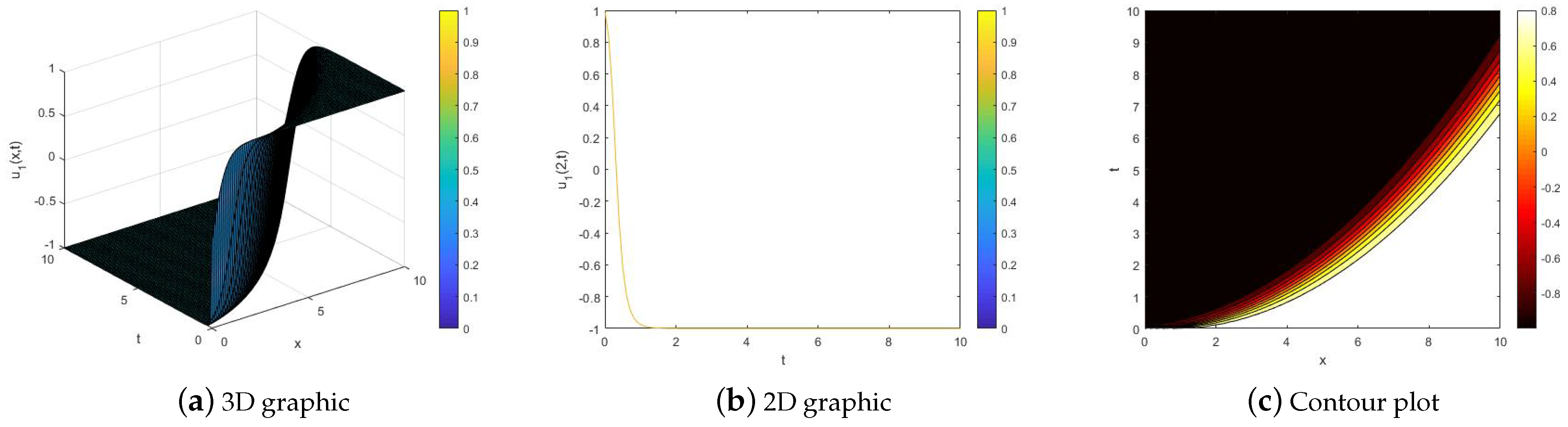
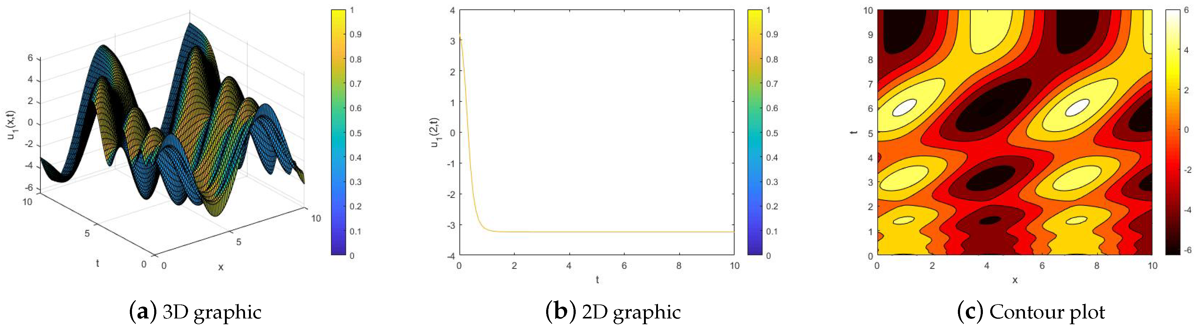
4. Numerical Simulation

In this section, we illustrate three-dimensional, two-dimensional, and contour maps of the modulus length as well as the real and imaginary parts of $u_1(x,t)$ when ${\zeta }_1=-1,{\zeta }_2=1,{\epsilon }_1=-1,$${\epsilon }_2=3,{\epsilon }_3=0,{\mu }_1=1,{\mu }_2=-4,{\chi }_1=2,{\chi }_2=2,{\chi }_3={\displaystyle \frac{1}{2}},C_1\ne 0,\alpha =\beta ={\displaystyle \frac{1}{2}}$, and $C_2=0$, as shown in Figure 1, Figure 2 and Figure 3. Moreover, we plot three-dimensional, two-dimensional, and contour maps of the modulus length as well as the real and imaginary parts of $u_5(x,t)$ when ${\zeta }_1=-1,$${\zeta }_2=1,{\epsilon }_1=-1,{\epsilon }_2=3,{\epsilon }_3=0,{\mu }_1=1,{\mu }_2=-4,{\chi }_1=2,{\chi }_2=1,{\chi }_3={\displaystyle \frac{1}{2}},C_1\ne 0,$$\alpha =\beta ={\displaystyle \frac{1}{2}}$, and $C_2=0$, as shown in Figure 4, Figure 5 and Figure 6.

5. Conclusions

In the article, we used the extended $(G^{\prime }/G)$-expansion method to study the optical solutions of NLKE-MTD. These solutions mainly include hyperbolic function solutions, rational function solutions, trigonometric function solutions, and negative power solutions. Moreover, we illustrated three-dimensional, two-dimensional, and contour maps of the modulus length as well as the real and imaginary parts of $u_1(x,t)$ and $u_5(x,t)$, respectively. Compared with [16], this paper considers the traveling wave solution of the fractional-order version of NLKE, and the $(G^{\prime }/G)$-expansion method used in this paper is an extended form method. In addition, this paper also provides solutions with negative power forms. These graphs clarify the propagation of waves in the solution of NLKE-MTD.

References

1. Alazman, I.; Alkahtani, B.S.T.; Mishra, M.N. Dynamic of bifurcation, chaotic structure and multi soliton of fractional nonlinear Schrödinger equation arise in plasma physics. Sci. Rep. 2024, 14, 25781. [Google Scholar] [CrossRef] [PubMed]
2. Li, Z.; Hussain, E. Qualitative analysis and traveling wave solutions of a (3+1)-dimensional generalized nonlinear Konopelchenko-Dubrovsky-Kaup-Kupershmidt system. Fractal Fract. 2025, 9, 285. [Google Scholar] [CrossRef]
3. Ali, A.; Senu, N.; Wahi, N.; Almakayeel, N.; Ahmadian, A. An adaptive algorithm for numerically solving fractional partial differential equations using Hermite wavelet artificial neural networks. Commun. Nonlinear Sci. 2024, 137, 108121. [Google Scholar] [CrossRef]
4. Jiang, Y.M.; Wang, X.C.; Wang, Y.J. On a stochastic heat equation with first order fractional noises and applications to finance. J. Math. Anal. Appl. 2012, 396, 656–669. [Google Scholar] [CrossRef]
5. Wilson, J.P.; Ji, C.; Dai, W.Z. A new variable-order fractional momentum operator for wave absorption when solving Schrödinger equations. J. Comput. Phys. 2024, 511, 113123. [Google Scholar] [CrossRef]
6. Xu, T.Z.; Liu, J.H.; Wang, Y.Y.; Dai, C.Q. Vector multipole solitons of fractional-order coupled saturable nonlinear Schrödinger equation. Chaos Solitons Fract. 2024, 186, 115230. [Google Scholar] [CrossRef]
7. Liu, C.Y. The traveling wave solution and dynamics analysis of the fractional order generalized Pochhammer–Chree equation. AIMS Math. 2024, 9, 33956–33972. [Google Scholar] [CrossRef]
8. Zhao, S. Chaos analysis and traveling wave solutions for fractional (3+1)-dimensional Wazwaz Kaur Boussinesq equation with beta derivative. Sci. Rep. 2024, 14, 23034. [Google Scholar] [CrossRef] [PubMed]
9. Li, C.Y. The Hautus-Type inequality for abstract fractional cauchy problems and its observability. J. Math. 2024, 2024, 6179980. [Google Scholar]
10. Li, C.Y. Zero-r Law on the analyticity and the uniform continuity of fractional resolvent families. Integr. Equ. Oper. Theory 2024, 96, 34. [Google Scholar]
11. Ye, Y.L.; Fan, H.T.; Li, Y.J.; Liu, X.Y.; Zhang, H.B. Deep neural network methods for solving forward and inverse problems of time fractional diffusion equations with conformable derivative. Neurocomputing 2022, 509, 177–192. [Google Scholar] [CrossRef]
12. Salah, B.; El-Zahar, E.R.; Aljohani, A.F.; Ebaid, A.; Krid, M. Optical soliton solutions of the time-fractional perturbed Fokas-Lenells equation: Riemann-Liouville fractional derivative. Optik 2019, 183, 1114–1119. [Google Scholar] [CrossRef]
13. Akram, G.; Sadaf, M.; Zainab, I. Observations of fractional effects of β-derivative and M-truncated derivative for space time fractional Phi-4 equation via two analytical techniques. Chaos Soliton Fract. 2022, 154, 111645. [Google Scholar] [CrossRef]
14. Zafar, A.; Bekir, A.; Raheel, M.; Razzaq, W. Optical soliton solutions to Biswas–Arshed model with truncated M-fractional derivative. Optik 2020, 222, 165355. [Google Scholar] [CrossRef]
15. Mohammed, W.W.; Iqbal, N.; Sidaoui, R.; Ali, E.E. Dynamical behavior of the fractional nonlinear Kodama equation in plasma physics and optics. Mod. Phys. Lett. B 2024, 39, 2450434. [Google Scholar] [CrossRef]
16. Algolam, M.S.; Ahmed, A.I.; Alshammary, H.M.; Mansour, F.E.; Mohammed, W.W. The impact of standard Wiener process on the optical solutions of the stochastic nonlinear Kodama equation using two different methods. J. Low Freq. Noise Vib. Act. Control 2024, 43, 1939–1952. [Google Scholar] [CrossRef]
17. Gu, M.S.; Liu, F.M.; Li, J.L.; Peng, C.; Li, Z. Explicit solutions of the generalized Kudryashov’s equation with truncated M-fractional derivative. Sci. Rep. 2024, 14, 21714. [Google Scholar] [CrossRef] [PubMed]
18. Luo, J.; Li, Z. Dynamic behavior and optical soliton for the M-Truncated fractional Paraxial wave equation arising in a liquid crystal model. Fractal Fract. 2024, 8, 348. [Google Scholar] [CrossRef]
19. Farooq, A.; Khan, M.I.Q.K.; Nisar, S.; Shah, N.A. A detailed analysis of the improved modified Korteweg-de Vries equation via the Jacobi elliptic function expansion method and the application of truncated M-fractional derivatives. Results Phys. 2024, 59, 107604. [Google Scholar] [CrossRef]
20. Li, Z.; Li, P.; Han, T.Y. White noise functional solutions for Wick-type stochastic fractional mixed KdV-mKdV equation using extended (G/G)-expansion method. Adv. Math. Phys. 2021, 2021, 9729905. [Google Scholar] [CrossRef]
Figure 1. The modulus of the solution u 1 ( x , t ) of Equation (1) for ζ 1 = 1 , ζ 2 = 1 , ε 1 = 1 , ε 2 = 3 , ε 3 = 0 , μ 1 = 1 , μ 2 = 4 , χ 1 = 2 , χ 2 = 2 , χ 3 = 1 2 , C 1 0 , C 2 = 0 , α = β = 1 2 .
Fractalfract 09 00300 g001
Figure 2. The real part of the solution u 1 ( x , t ) of Equation (1) for ζ 1 = 1 , ζ 2 = 1 , ε 1 = 1 , ε 2 = 3 , ε 3 = 0 , μ 1 = 1 , μ 2 = 4 , χ 1 = 2 , χ 2 = 2 , χ 3 = 1 2 , C 1 0 , C 2 = 0 , α = β = 1 2 .
Fractalfract 09 00300 g002
Figure 3. The imaginary part of the solution u 1 ( x , t ) of Equation (1) for ζ 1 = 1 , ζ 2 = 1 , ε 1 = 1 , ε 2 = 3 , ε 3 = 0 , μ 1 = 1 , μ 2 = 4 , χ 1 = 2 , χ 2 = 2 , χ 3 = 1 2 , C 1 0 , C 2 = 0 , α = β = 1 2 .
Fractalfract 09 00300 g003
Figure 4. The modulus of the solution u 5 ( x , t ) of Equation (1) for ζ 1 = 1 , ζ 2 = 1 , ε 1 = 1 , ε 2 = 3 , ε 3 = 0 , μ 1 = 1 , μ 2 = 4 , χ 1 = 2 , χ 2 = 1 , χ 3 = 1 2 , C 1 0 , C 2 = 0 , α = β = 1 2 .
Fractalfract 09 00300 g004
Figure 5. The real part of the solution u 5 ( x , t ) of Equation (1) for ζ 1 = 1 , ζ 2 = 1 , ε 1 = 1 , ε 2 = 3 , ε 3 = 0 , μ 1 = 1 , μ 2 = 4 , χ 1 = 2 , χ 2 = 1 , χ 3 = 1 2 , C 1 0 , C 2 = 0 , α = β = 1 2 .
Fractalfract 09 00300 g005
Figure 6. The imaginary part of the solution u 5 ( x , t ) of Equation (1) for ζ 1 = 1 , ζ 2 = 1 , ε 1 = 1 , ε 2 = 3 , ε 3 = 0 , μ 1 = 1 , μ 2 = 4 , χ 1 = 2 , χ 2 = 1 , χ 3 = 1 2 , C 1 0 , C 2 = 0 , α = β = 1 2 .
Fractalfract 09 00300 g006
Disclaimer/Publisher’s Note: The statements, opinions and data contained in all publications are solely those of the individual author(s) and contributor(s) and not of MDPI and/or the editor(s). MDPI and/or the editor(s) disclaim responsibility for any injury to people or property resulting from any ideas, methods, instructions or products referred to in the content.