On Solving Modified Time Caputo Fractional Kawahara Equations in the Framework of Hilbert Algebras Using the Laplace Residual Power Series Method

Abstract

In this work, we first develop the modified time Caputo fractional Kawahara Equations (MTCFKEs) in the usual Hilbert spaces and extend them to analogous structures within the theory of Hilbert algebras. Next, we employ the residual power series method, combined with the Laplace transform, to introduce a new effective technique called the Laplace Residual Power Series Method (LRPSM). This method is applied to derive the coefficients of the series solution for MTCFKEs in the context of Hilbert algebras. In real Hilbert algebras, we obtain approximate solutions for MTCFKEs under both exact and approximate initial conditions. We present both graphical and numerical results of the approximate analytical solutions to demonstrate the capability, efficiency, and reliability of the LRPSM. Furthermore, we compare our results with solutions obtained using the homotopy analysis method and the natural transform decomposition method.

1. Introduction

The theory of wave differential equations is regarded as a fundamental concept in physics, fluid dynamics, mathematics, and other fields. In the context of real Hilbert space $\mathbb{R}$, the following equation emerges:

$$\left\{\begin{array}{c}{\displaystyle \frac{\partial \lambda (\vartheta ,\nu )}{\partial \nu }}+\lambda (\vartheta ,\nu ){\displaystyle \frac{\partial \lambda (\vartheta ,\nu )}{\partial \vartheta }}+{\displaystyle \frac{{\partial }^3\lambda (\vartheta ,\nu )}{\partial {\vartheta }^3}}-{\displaystyle \frac{{\partial }^5\lambda (\vartheta ,\nu )}{\partial {\vartheta }^5}}=0\hfill \\ \lambda (\vartheta ,0)=h_0\left(\vartheta \right).\hfill \end{array}\right.$$

(1)

This is called time Kawahara equation, which is the most one of the wave equations introduced by Kawahara in 1970 [1]. Kawahara equations are introduced to characterize solitary wave propagation in various media [2,3,4]. Within the study of waves, we find theories such as shallow water waves and magneto-acoustic waves. The theory of shallow water wave equations has been widely applied in several scientific fields to model phenomena such as tsunami propagation, shock waves, and storm surges. Additionally, many generalizations of the conservation and symmetry laws of the Kawahara equation have been presented by Jakub [5]. For applications of the Kawahara equations in the theory of plasma waves and capillary gravity water waves, several studies have been conducted. For more details, see [6,7,8,9]. Given the significant importance of shallow water wave equations in various sciences, researchers in recent years have employed various numerical and analytical methods to obtain approximate solutions. These methods include the finite element method, finite volume method, homotopy perturbation method, finite difference method, variational iteration method, and Adomian decomposition method, among others. On another note, the theory of fractional calculus has gained importance in recent years. Numerous results and fractional operators have emerged to support mathematical modeling, particularly to describe the hereditary properties of processes and materials. Partial fractional differential equations serve as effective representations for various modeling applications in physics, groundwater problems, electrical networks, fluid mechanics, medicine, engineering, and polymer science [10,11,12]. The time Caputo fractional Kawahara equation (TCFKE) and its modified version, the modified time Caputo fractional Kawahara equation (MTCFKE), are notable examples of these partial fractional differential equations.

$$\left\{\begin{array}{c}{}^C\mathcal{D}_{0,\nu }^{\varrho }\lambda (\vartheta ,\nu )+\lambda (\vartheta ,\nu ){\displaystyle \frac{\partial \lambda (\vartheta ,\nu )}{\partial \vartheta }}+{\displaystyle \frac{{\partial }^3\lambda (\vartheta ,\nu )}{\partial {\vartheta }^3}}-{\displaystyle \frac{{\partial }^5\lambda (\vartheta ,\nu )}{\partial {\vartheta }^5}}=0,0<\varrho \le 1\hfill \\ \lambda (\vartheta ,0)=f_0\left(\vartheta \right)\hfill \end{array}\right.$$

(2)

and

$$\left\{\begin{array}{c}{}^C\mathcal{D}_{0,\nu }^{\varrho }\lambda (\vartheta ,\nu )+{\lambda }^2(\vartheta ,\nu ){\displaystyle \frac{\partial \lambda (\vartheta ,\nu )}{\partial \vartheta }}+\alpha {\displaystyle \frac{{\partial }^3\lambda (\vartheta ,\nu )}{\partial {\vartheta }^3}}+\beta {\displaystyle \frac{{\partial }^5\lambda (\vartheta ,\nu )}{\partial {\vartheta }^5}}=0,0<\varrho \le 1\hfill \\ \lambda (\vartheta ,0)=h_0\left(\vartheta \right),\hfill \end{array}\right.$$

(3)

respectively, where ${}^C\mathcal{D}_{0,\nu }^{\varrho }$ is the Caputo fractional derivative of order $\varrho$ and $\alpha >0$, $\beta <0$ are constants. For various physical systems and biological equations, several researchers used fractional calculus of some partial differential equations and mathematical methods to obtain and examine the approximate or exact solutions. In the real Hilbert space $\mathbb{R}$ and complex Hilbert space $\mathbb{C}$, several methods and efficient techniques have been used to obtain approximate and exact solutions of fractional differential equations in engineering, physics, and biology, for example, the Laplace transform method was used with fuzzy partial differential Equations [13], the expansion method with higher-order nonlinear Boussinesq-type wave equation transform [14], fractional Newton method for 2$\varrho$-order of convergence and its stability [15], the sine–Gordon expansion method with Wu–Zhang system models [16], and the homotopy analysis method [17]. Other examples include reproducing the kernel Hilbert space method with the telegraph equation [18], Fornberg–Whitham-type equation [19], and non-local fractional equation [20]. A monotone iterative method with a reaction diffusion equation [21], a variational iteration method with some non-linear fractional differential equations [22], and a homotopy perturbation method with some equations [23] were also used. Other examples include the modified expansion function method with the non-linear Schrodinger equation [24], a modified Adams–Bashforth method with an Atangana–Baleanu Caputo fractional equation [25], and an extended direct algebraic mapping method with nonlinear damped modified Korteweg–de Vries Equation [26].

In the context of Hilbert spaces, some approximate and exact solutions for MTCFKE are introduced by using several techniques and methods, such as an iterative Laplace transform method [27] and the homotopy analysis method [28]. Kaur and Gupta [29] used Lie group analysis to study variable coefficients in the Kawahara equation and variable coefficients in the modified Kawahara equation of various physical phenomena. Ak and Karakoc [30] used the septic B-spline collocation method to obtain some numerical solutions of the modified Kawahara equations. Bhatter et al. [31] proved the existence and uniqueness of the approximate solution of the fractional modified Kawahara equation by using the fixed-point theorem. They used homotopy analysis transform technique to obtain the solution of the fractional modified Kawahara equation. The natural transform method [32] and the residual power series method [33], followed the Laplace Adomian decomposition method [34].

Khater [35], elucidated the nuanced behavior inherent in the generalized Kawahara equation and deployed two robust analytical methodologies.

There are many mathematical methods that have been introduced in obtaining and examining the approximate results of partial differential equations. The LRPSM is one of theses methods where the technique of LRPSM was used by several researchers to obtain the approximate and exact solutions of differential equations such as that of Shafee et al. [36], who introduced an efficient method for solving fractional system partial differential equations using the LRPSM, proving that the LRPSM is a reliable and efficient method for solving fractional system partial differential equations. Albalawi et al. [37] introduced the approximate and exact solutions of the fractional three-dimensional (3D) Helmholtz equation and examined the relationship between the actual solutions and the derived solutions. They proved the number of terms in the series solution of the problems increases by showing that the approximate solution converges to the actual solution. Oqielat et al. [38] presented some approximate solutions for the nonlinear time-fractional reaction–diffusion equations. Khresat et al. [39] utilized the LRPSM to introduce some analytic solutions to various kinds of partial differential equations, and they derived certain solutions to different types of linear and nonlinear partial differential equations, including wave equations, non-homogeneous space telegraph equations, water wave partial differential equations, Klein–Gordon partial differential equations, Fisher equations, and a few others. They also examined these numerically and compared the obtained results with some known approximate solutions.

Recall [40] that the Banach algebra is a collection of a Banach space $\mathcal{B}$ over a field $\mathbb{F}$ and a norm $\left|\right|·\left|\right|$ on $\mathcal{B}$ with an associative and distributive multiplication on $\mathcal{B}$, such that $r\left(ab\right)=\left(ra\right)b=a\left(rb\right)$ for all $a,b\in \mathcal{B}$, $r\in \mathbb{F}$ and the operation $\mathcal{B}\times \mathcal{B}\to \mathcal{B}:(a,b)\to ab$ is a continuous function with respect to the mertizable topological space induced $\left|\right|.\left|\right|$. Note that the Banach algebra $\mathcal{B}$ is topological semigroup and $\left|\right|ab\left|\right|\le \left|\right|a\left|\right|\left|\right|b\left|\right|$ for all $a,b\in \mathcal{B}$. It is clear that every Hilbert space with the norm induced by its inner product is a Banach space. By Hibert algebra $\mathcal{H}$, we mean the Hilbert space $\mathcal{H}$ that forms Banach algebra with the norm induced by its inner product. Let $\mathcal{H}$ be a Hilbert algebra over a field $\mathbb{F}$ and an inner product $⟨·,·⟩$. Let $\lambda (\vartheta ,\nu ):I\times [0,\infty )\to \mathcal{H}$ be any function on $\mathbb{J}:=I\times [0,\infty )$ where I is any interval on real space $\mathbb{R}$. In this work, our motivation is obtaining some solutions that are more approximate to the exact solution of the following MTCFKE:

$$\left\{\begin{array}{c}{}^C\mathcal{D}_{0,\nu }^{\varrho }\lambda (\vartheta ,\nu )+{\lambda }^p(\vartheta ,\nu ){\displaystyle \frac{\partial \lambda (\vartheta ,\nu )}{\partial \vartheta }}+{\left[\lambda (\vartheta ,\nu )\right]}_{\beta \alpha }=0,0<\varrho \le 1\hfill \\ \lambda (\vartheta ,0)=h_0\left(\vartheta \right),\hfill \end{array}\right.$$

(4)

where $p\in \mathbb{N}$, $a^p=aa\cdots a\left(ptimes\right)$ for all $a\in \mathcal{H}$,

$${\left[\lambda (\vartheta ,\nu )\right]}_{\beta \alpha }=\alpha {\displaystyle \frac{{\partial }^3\lambda (\vartheta ,\nu )}{\partial {\vartheta }^3}}+\beta {\displaystyle \frac{{\partial }^5\lambda (\vartheta ,\nu )}{\partial {\vartheta }^5}}+\left[{\displaystyle \frac{{\partial }^3\lambda }{\partial {\vartheta }^3}},{\displaystyle \frac{{\partial }^5\lambda }{\partial {\vartheta }^5}}\right](\vartheta ,\nu ),$$

$\alpha ,\beta \in \mathbb{F}$, ${}^C\mathcal{D}_{0,\nu }^{\varrho }$ is the Caputo fractional derivative of order $\varrho$ and $[·,·]:C(\mathbb{J},\mathcal{H})\times C(\mathbb{J},\mathcal{H})\to C(\mathbb{J},\mathcal{H})$ is a Lie bracket operator which is defined by

$$[\lambda ,\mu ](\vartheta ,\nu )=\lambda (\vartheta ,\nu )\mu (\vartheta ,\nu )-\mu (\vartheta ,\nu )\lambda (\vartheta ,\nu ).$$

We investigate and introduce the technique of the LRPSM to find these approximate solutions. In Section 2, we recall the basic concepts and facts that concern Laplace transom and Caputo fractional differential operators. In Section 3, we introduce the basic preliminaries of the LRPSM. In Section 4, we investigate and introduce the exact and approximate solutions of the MTCFKE (4) by using the technique of the LRPSM. The approximate solutions of the MTCFKE (4) are introduced in two cases; the first case is with the exact initial condition of the MTCFKE (4), and the second with approximate initial condition of the MTCFKE (4). In Section 5, we present our results numerically in some tables and graphically in some curves and surface plots. We explain some comparisons among our results and some known previous results concerning the approximate solutions of some MTCFKEs, which were obtained by using homotopy analysis in [28] and the natural transform decomposition method [32]. In Section 6, we present some discussion and conclusions.

2. Preliminaries

Let $\lambda (\vartheta ,\nu )$ be any piecewise continuous on $\mathbb{J}:=I\times [0,\infty )$, where I is any interval on real space $\mathbb{R}$. The Riemann–Liouville fractional derivative [41] for $\lambda (\vartheta ,\nu )$ in the order of $\varrho >0$ is given by

$${\mathcal{D}}_{0,\nu }^{\varrho }\lambda (\vartheta ,\nu )={\mathcal{D}}_{\nu }^n{\mathcal{I}}_{0,\nu }^{\varrho }\lambda (\vartheta ,\nu )n-1<\varrho <n$$

(5)

where $n\in \mathbb{N}$ and ${\mathcal{I}}_{0,\nu }^{\varrho }$ is the Riemann–Liouville fractional integral [42] for $\lambda (\vartheta ,\nu )$ in the order of $\varrho$ is given by

$${\mathcal{I}}_{0,\nu }^{\varrho }\lambda (\vartheta ,\nu )=\left\{\begin{array}{c}{\displaystyle \frac{1}{\Gamma \left(\varrho \right)}}{\int }_0^{\nu }{(\nu -\mathcal{T})}^{\varrho -1}\lambda (\vartheta ,\mathcal{T})d\mathcal{T},\varrho >0\hfill \\ \lambda (\vartheta ,\nu ),\varrho =0.\hfill \end{array}\right.$$

(6)

The Caputo fractional derivative [36] for $\lambda (\vartheta ,\nu )$ is the order of $\varrho$ is given by

$${}^C\mathcal{D}_{0,\nu }^{\varrho }\lambda (\vartheta ,\nu )=\left\{\begin{array}{c}{\mathcal{I}}_{0,\nu }^{n-\varrho }\left[{\displaystyle \frac{{\partial }^n\lambda (\vartheta ,\nu )}{\partial {\nu }^n}}\right],n-1<\varrho <n\hfill \\ {\displaystyle \frac{{\partial }^{\varrho }\lambda (\vartheta ,\nu )}{\partial {\nu }^{\varrho }}},\varrho \in \mathbb{N},\hfill \end{array}\right.$$

(7)

Recall [38] that for $\nu \ge 0$ and for $n-1<\varrho <n$, we have ${}^C\mathcal{D}_{0,\nu }^{\varrho }{\mathcal{I}}_{0,\nu }^{\varrho }\lambda (\vartheta ,\nu )=\lambda (\vartheta ,\nu )$, ${}^C\mathcal{D}_{0,\nu }^{\varrho }{\nu }^{\gamma }={\displaystyle \frac{\Gamma (\varrho +1)}{\Gamma (\gamma -\varrho +1)}}{\nu }^{\gamma -\varrho }$ and

$${\mathcal{I}}_{0,\nu }^{\varrho }{}^C\mathcal{D}_{0,\nu }^{\varrho }\lambda (\vartheta ,\nu )=\lambda (\vartheta ,\nu )+\sum _{k=0}^{n-1}{\displaystyle \frac{{\nu }^k}{k!}}{\displaystyle \frac{{\partial }^k\lambda (\vartheta ,\nu )}{\partial {\nu }^k}}{|}_{\nu =0},$$

where $c\in \mathbb{R}$ is a constant, $n\in \mathbb{N}$, and $\gamma >-1$.

Let I be any interval on $\mathbb{R}$. Let $\lambda (\vartheta ,\nu )$ be any piecewise continuous function on $I\times [0,\infty )$ and of exponential order $\rho$. The Laplace transform $L_{\nu }$ [43] of $\lambda (\vartheta ,\nu )$ with respect to $\nu$ is given by

$${\lambda }_{\nu }(\vartheta ,\eta ):=L_{\nu }\lambda (\vartheta ,\nu )={\int }_0^{\infty }{e}^{-\nu \eta }\lambda (\vartheta ,\eta )d\eta \eta >\rho .$$

(8)

The inverse Laplace transform $L_{\nu }^{-1}$ of ${\lambda }_{\nu }(\vartheta ,\eta )$ with respect to $\eta$ is given by

$$\lambda (\vartheta ,\nu ):=L_{\nu }^{-1}{\lambda }_{\nu }(\vartheta ,\eta )={\int }_{\Re \left(\eta \right)-i\infty }^{\Re \left(\eta \right)+i\infty }{e}^{\nu \eta }\lambda (\vartheta ,\eta )d\eta \Re \left(\eta \right)>b_0,$$

(9)

where $b_0$ belongs to the right half plane of the absolute convergence of the Laplace integral. Let $\lambda (\vartheta ,\nu )$ and $\mu (\vartheta ,\nu )$ be two piecewise continuous functions on $I\times [0,\infty )$ of exponential orders ${\rho }_1$ and ${\rho }_2$ (${\rho }_1<{\rho }_2$), respectively. Recall [43] that the Laplace transform $L_{\nu }$ has the following properties:

• $L_{\nu }[c_1\lambda (\vartheta ,\nu )+c_2\mu (\vartheta ,\nu )]=c_1{L}_{\nu }\lambda (\vartheta ,\nu )+c_2{L}_{\nu }\mu (\vartheta ,\nu )$ for all $\vartheta \in I$ and $\nu >{\rho }_1$, where $c_1$ and $c_2$ are constants;
• $L_{\nu }\left[e^{c\nu }\lambda (\vartheta ,\nu )\right]={\lambda }_{\nu }(\vartheta ,\eta -c)$ for all $\vartheta \in I$ and $\nu >{\rho }_1+c$, where c is constant;
• ${lim}_{\eta \to \infty }\eta {\lambda }_{\nu }(\vartheta ,\eta )=\lambda (\vartheta ,0)$ for all $\vartheta \in I$.

In the following lemma, we explain the Laplace transform of the Caputo fractional operator.

Lemma 1

([38]). Let $\lambda (\vartheta ,\nu )$ be a piecewise continuous function on $I\times [0,\infty )$ of exponential order ρ. Then,

• $L_{\nu }\left[{}^C\mathcal{D}_{0,\nu }^{\varrho }\lambda (\vartheta ,\nu )\right]={\eta }^{\varrho }{\lambda }_{\nu }(\vartheta ,\eta )-{\sum }_{j=0}^{n-1}{\eta }^{\varrho -j-1}{\partial }_{\nu }^j\lambda (\vartheta ,\nu ){|}_{\nu =0}$$(n-1<\varrho <n)$;
• $L_{\nu }\left[{}^C\mathcal{D}_{0,\nu }^{k\varrho }\lambda (\vartheta ,\nu )\right]={\eta }^{k\varrho }{\lambda }_{\nu }(\vartheta ,\eta )-{\sum }_{j=0}^{k-1}{\eta }^{(k-j)\varrho -1}{}^C\mathcal{D}_{0,\nu }^{j\varrho }\lambda (\vartheta ,\nu ){|}_{\nu =0}$$(0<\varrho \le 1).$

Theorem 1

([37]). Let $\lambda (\vartheta ,\nu )$ be a piecewise continuous function on $I\times [0,\infty )$ of exponential order ρ. Then,

$$L_{\nu }\left[{}^C\mathcal{D}_{0,\nu }^{\varrho }\lambda (\vartheta ,\nu )\right]=\sum _{j=0}^{\infty }{\displaystyle \frac{f_j\left(\vartheta \right)}{{\eta }^{j\varrho +1}}}(0<\varrho \le 1)$$

for all $\vartheta \in I$ and $\eta >\rho$, where $f_j\left(\vartheta \right)={}^C\mathcal{D}_{0,\nu }^{j\varrho }\lambda (\vartheta ,\nu ){|}_{\nu =0}$.

In the theorem above, the inverse Laplace transform is given by the following:

$$\lambda (\vartheta ,\nu )=\sum _{j=0}^{\infty }{\displaystyle \frac{{}^C\mathcal{D}_{0,\nu }^{j\varrho }\lambda (\vartheta ,\nu ){|}_{\nu =0}}{\Gamma (j\varrho +1)}}{\nu }^{j\varrho }(0<\varrho \le 1)$$

for all $\vartheta \in I$ and $\nu >0$.

3. The Methodology of the LRPSM

In this section, we recall the steps of the LRPSM [36] in solving partial differential equations of fractional orders. Consider the following MTCFKE in Equation (4):

$$\left\{\begin{array}{c}{}^C\mathcal{D}_{0,\nu }^{\varrho }\lambda (\vartheta ,\nu )+{\lambda }^p(\vartheta ,\nu ){\displaystyle \frac{\partial \lambda (\vartheta ,\nu )}{\partial \vartheta }}+{\left[\lambda (\vartheta ,\nu )\right]}_{\beta \alpha }=0,0<\varrho \le 1\hfill \\ \lambda (\vartheta ,0)=h_0\left(\vartheta \right),\hfill \end{array}\right.$$

(10)

where

$${\left[\lambda (\vartheta ,\nu )\right]}_{\beta \alpha }=\alpha {\displaystyle \frac{{\partial }^3\lambda (\vartheta ,\nu )}{\partial {\vartheta }^3}}+\beta {\displaystyle \frac{{\partial }^5\lambda (\vartheta ,\nu )}{\partial {\vartheta }^5}}+\left[{\displaystyle \frac{{\partial }^3\lambda }{\partial {\vartheta }^3}},{\displaystyle \frac{{\partial }^5\lambda }{\partial {\vartheta }^5}}\right](\vartheta ,\nu ).$$

Use the Laplace transform $L_{\nu }$ of Equation (10)

$$L_{\nu }\left[{}^C\mathcal{D}_{0,\nu }^{\varrho }\lambda (\vartheta ,\nu )\right]+L_{\nu }\left[{\lambda }^p(\vartheta ,\nu ){\displaystyle \frac{\partial \lambda (\vartheta ,\nu )}{\partial \vartheta }}\right]+L_{\nu }\left[{\left[\lambda (\vartheta ,\nu )\right]}_{\beta \alpha }\right]=0.$$

(11)

By Lemma 1, the Laplace transform $L_{\nu }\left[{}^C\mathcal{D}_{0,\nu }^{\varrho }\lambda (\vartheta ,\nu )\right]$ in the left side of Equation (10) becomes

$$L_{\nu }\left[{}^C\mathcal{D}_{0,\nu }^{\varrho }\lambda (\vartheta ,\nu )\right]={\eta }^{\varrho }{\lambda }_{\nu }(\vartheta ,\eta )-{\eta }^{\varrho -1}{h}_0\left(\vartheta \right).$$

(12)

Then, from Equations (11) and (12) we obtain that

$$\begin{array}{cc}\hfill & {\lambda }_{\nu }(\vartheta ,\eta )={\displaystyle \frac{1}{\eta }}{h}_0\left(\vartheta \right)-{\displaystyle \frac{1}{{\eta }^{\varrho }}}{L}_{\nu }\left[{\left[L_{\nu }^{-1}\left({\lambda }_{\nu }(\vartheta ,\eta )\right)\right]}^p{\displaystyle \frac{{\partial }^3{L}_{\nu }^{-1}\left({\lambda }_{\nu }(\vartheta ,\eta )\right)}{\partial {\vartheta }^3}}\right]\hfill \\ \hfill & -{\displaystyle \frac{1}{{\eta }^{\varrho }}}{L}_{\nu }\left[{\lambda }_{\nu }{(\vartheta ,\eta )}_{\beta \alpha }\right]\hfill \end{array}$$

(13)

where

$$\begin{array}{cc}\hfill & {\lambda }_{\nu }{(\vartheta ,\eta )}_{\beta \alpha }=\alpha L_{\nu }\left[{\displaystyle \frac{{\partial }^3{L}_{\nu }^{-1}\left({\lambda }_{\nu }(\vartheta ,\eta )\right)}{\partial {\vartheta }^3}}\right]+\beta L_{\nu }\left[{\displaystyle \frac{{\partial }^5{L}_{\nu }^{-1}\left({\lambda }_{\nu }(\vartheta ,\eta )\right)}{\partial {\vartheta }^5}}\right]\hfill \\ \hfill & +L_{\nu }\left[{\displaystyle \frac{{\partial }^3{L}_{\nu }^{-1}\left({\lambda }_{\nu }(\vartheta ,\eta )\right)}{\partial {\vartheta }^3}}\right]L_{\nu }\left[{\displaystyle \frac{{\partial }^5{L}_{\nu }^{-1}\left({\lambda }_{\nu }(\vartheta ,\eta )\right)}{\partial {\vartheta }^5}}\right]\hfill \\ \hfill & -L_{\nu }\left[{\displaystyle \frac{{\partial }^5{L}_{\nu }^{-1}\left({\lambda }_{\nu }(\vartheta ,\eta )\right)}{\partial {\vartheta }^5}}\right]L_{\nu }\left[{\displaystyle \frac{{\partial }^3{L}_{\nu }^{-1}\left({\lambda }_{\nu }(\vartheta ,\eta )\right)}{\partial {\vartheta }^3}}\right].\hfill \end{array}$$

(14)

Let the following power series be a solution for Equation (11):

$${\lambda }_{\nu }(\vartheta ,\eta )=\sum _{j=0}^{\infty }{\displaystyle \frac{h_j\left(\vartheta \right)}{{\eta }^{j\varrho +1}}}.$$

(15)

By Lemma 1 and by the initial condition in Equation (10), we can write the partial sums sequence ${⟨{\lambda }_{\nu n}⟩}_{n\in \mathbb{N}\cup \left\{0\right\}}$ of the series above in Equation (15) as

$${\lambda }_{\nu n}(\vartheta ,\eta )={\displaystyle \frac{1}{\eta }}{h}_0\left(\vartheta \right)+\sum _{j=1}^n{\displaystyle \frac{h_j\left(\vartheta \right)}{{\eta }^{j\varrho +1}}}.$$

(16)

Next, construct the Laplace residual function $L_{\nu }\mathcal{R}es\lambda (\vartheta ,\eta )$ for Equation (13) as follows:

$$\begin{array}{cc}\hfill & L_{\nu }\mathcal{R}es\lambda (\vartheta ,\eta )={\lambda }_{\nu }(\vartheta ,\eta )-{\displaystyle \frac{1}{\eta }}{h}_0\left(\vartheta \right)\hfill \\ \hfill & +{\displaystyle \frac{1}{{\eta }^{\varrho }}}{L}_{\nu }\left[{\left[L_{\nu }^{-1}\left({\lambda }_{\nu }(\vartheta ,\eta )\right)\right]}^p{\displaystyle \frac{{\partial }^3{L}_{\nu }^{-1}\left({\lambda }_{\nu }(\vartheta ,\eta )\right)}{\partial {\vartheta }^3}}\right]+{\displaystyle \frac{1}{{\eta }^{\varrho }}}{L}_{\nu }\left[{\lambda }_{\nu }{(\vartheta ,\eta )}_{\beta \alpha }\right]\hfill \end{array}$$

(17)

and the n-th Laplace residual function $L_{\nu }\mathcal{R}e{s}_n\lambda (\vartheta ,\eta )$ is

$$\begin{array}{cc}\hfill & L_{\nu }\mathcal{R}e{s}_n\lambda (\vartheta ,\eta )={\lambda }_{\nu n}(\vartheta ,\eta )-{\displaystyle \frac{1}{\eta }}{h}_0\left(\vartheta \right)\hfill \\ \hfill & +{\displaystyle \frac{1}{{\eta }^{\varrho }}}{L}_{\nu }\left[{\left[L_{\nu }^{-1}\left({\lambda }_{\nu n}(\vartheta ,\eta )\right)\right]}^p{\displaystyle \frac{{\partial }^3{L}_{\nu }^{-1}\left({\lambda }_{\nu n}(\vartheta ,\eta )\right)}{\partial {\vartheta }^3}}\right]+{\displaystyle \frac{1}{{\eta }^{\varrho }}}{L}_{\nu }\left[{\lambda }_{\nu n}{(\vartheta ,\eta )}_{\beta \alpha }\right]\hfill \end{array}$$

(18)

where

$$\begin{array}{cc}\hfill & {\lambda }_{\nu n}{(\vartheta ,\eta )}_{\beta \alpha }=\alpha L_{\nu }\left[{\displaystyle \frac{{\partial }^3{L}_{\nu }^{-1}\left({\lambda }_{\nu n}(\vartheta ,\eta )\right)}{\partial {\vartheta }^3}}\right]+\beta L_{\nu }\left[{\displaystyle \frac{{\partial }^5{L}_{\nu }^{-1}\left({\lambda }_{\nu n}(\vartheta ,\eta )\right)}{\partial {\vartheta }^5}}\right]\hfill \\ \hfill & +L_{\nu }\left[{\displaystyle \frac{{\partial }^3{L}_{\nu }^{-1}\left({\lambda }_{\nu n}(\vartheta ,\eta )\right)}{\partial {\vartheta }^3}}\right]L_{\nu }\left[{\displaystyle \frac{{\partial }^5{L}_{\nu }^{-1}\left({\lambda }_{\nu n}(\vartheta ,\eta )\right)}{\partial {\vartheta }^5}}\right]\hfill \\ \hfill & -L_{\nu }\left[{\displaystyle \frac{{\partial }^5{L}_{\nu }^{-1}\left({\lambda }_{\nu n}(\vartheta ,\eta )\right)}{\partial {\vartheta }^5}}\right]L_{\nu }\left[{\displaystyle \frac{{\partial }^3{L}_{\nu }^{-1}\left({\lambda }_{\nu n}(\vartheta ,\eta )\right)}{\partial {\vartheta }^3}}\right].\hfill \end{array}$$

(19)

Next, we recall some facts and properties of the typical residual power series approach as follows[36]: Note that $L_{\nu }\mathcal{R}es\lambda (\vartheta ,\eta )=0$ and ${lim}_{n\to \infty }{L}_{\nu }\mathcal{R}e{s}_n\lambda (\vartheta ,\eta )=L_{\nu }\mathcal{R}es\lambda (\vartheta ,\eta )$ for all $\eta >0$. Note that if ${lim}_{\eta \to \infty }\eta L_{\nu }\mathcal{R}es\lambda (\vartheta ,\eta )=0$, then ${lim}_{\eta \to \infty }\eta L_{\nu }\mathcal{R}e{s}_n\lambda (\vartheta ,\eta )=0$. In general,

$$\underset{\eta \to \infty }{lim}{\eta }^{n\varrho +1}{L}_{\nu }\mathcal{R}es\lambda (\vartheta ,\eta )=\underset{\eta \to \infty }{lim}{\eta }^{n\varrho +1}{L}_{\nu }\mathcal{R}e{s}_n\lambda (\vartheta ,\eta )=0$$

for all $n=1,2,3,\cdots$ and $0<\varrho \le 1$. To obtain the coefficients $h_n\left(\vartheta \right)$, we apply the iterative method to solve the following system:

$$\underset{\eta \to \infty }{lim}{\eta }^{n\varrho +1}{L}_{\nu }\mathcal{R}e{s}_n\lambda (\vartheta ,\eta )=0$$

(20)

for all $n=1,2,3,\cdots$. Next, we substitute the forms of the coefficients, $h_n\left(\vartheta \right)$ into Equation (16) to obtain the n-th proximate solutions ${\lambda }_{\nu n}(\vartheta ,\eta )$ of Equation (13). Finally, we use the inverse Laplace transform of the n-th proximate solutions ${\lambda }_{\nu n}(\vartheta ,\eta )$ to obtain the existence of the n-th proximate solutions ${\lambda }_{\nu }^n(\vartheta ,\nu )$ of Equation (10).

4. Approximate Solutions

It is clear that the Banach space $\mathbb{R}$ is commutative Hilbert algebra with the usual multiplication and with the norm $\left|\right|\iota \left|\right|=\left|\iota \right|$. That is, the Lie bracket operator is equal to the zero operator. Hence, in the MTCFKE (4), the part ${\left[\lambda (\vartheta ,\nu )\right]}_{\beta \alpha }$ will be

$${\left[\lambda (\vartheta ,\nu )\right]}_{\beta \alpha }=\alpha {\displaystyle \frac{{\partial }^3\lambda (\vartheta ,\nu )}{\partial {\vartheta }^3}}+\beta {\displaystyle \frac{{\partial }^5\lambda (\vartheta ,\nu )}{\partial {\vartheta }^5}}.$$

In this section, we introduce and instigate some approximate and exact solutions of the MTCFKE (4) in Hilbert algebra $\mathbb{R}$ with $p=2$ by using the technique of the LRPSM above. To obtain these solutions, we start by taking this MTCFKE with the exact initial condition of the MTCFKE and then take it with the approximate initial condition.

Consider the following MTCFKE

$$\left\{\begin{array}{c}{}^C\mathcal{D}_{0,\nu }^{\varrho }\lambda (\vartheta ,\nu )+{\lambda }^2(\vartheta ,\nu ){\displaystyle \frac{\partial \lambda (\vartheta ,\nu )}{\partial \vartheta }}+\alpha {\displaystyle \frac{{\partial }^3\lambda (\vartheta ,\nu )}{\partial {\vartheta }^3}}+\beta {\displaystyle \frac{{\partial }^5\lambda (\vartheta ,\nu )}{\partial {\vartheta }^5}}=0,0<\varrho \le 1\hfill \\ \lambda (\vartheta ,0)={\displaystyle \frac{3\alpha }{\sqrt{-10\beta }}}{\mathrm{sech}}^2\left({\displaystyle \frac{1}{2}}\sqrt{{\displaystyle \frac{-\alpha }{5\beta }}}\vartheta \right)\hfill \end{array}\right.$$

(21)

where $\alpha >0$, $\beta <0$ are constants. Recall [28] that if $\varrho =1$, then the exact solution of the MTCFKE (21) is given by

$$\lambda (\vartheta ,\nu )={\displaystyle \frac{3\alpha }{\sqrt{-10\beta }}}{\mathrm{sech}}^2\left[{\displaystyle \frac{1}{2}}\sqrt{{\displaystyle \frac{-\alpha }{5\beta }}}\left(\vartheta -{\displaystyle \frac{25\beta -4{\alpha }^2}{25\beta }}\nu \right)\right].$$

(22)

Use Laplace transforms on Equation (21) to obtain the following equation:

$$\begin{array}{cc}\hfill & {\lambda }_{\nu }(\vartheta ,\eta )={\displaystyle \frac{3\alpha }{\eta \sqrt{-10\beta }}}{\mathrm{sech}}^2\left({\displaystyle \frac{1}{2}}\sqrt{{\displaystyle \frac{-\alpha }{5\beta }}}\vartheta \right)\hfill \\ & -{\displaystyle \frac{1}{{\eta }^{\varrho }}}{L}_{\nu }\left[{\left[L_{\nu }^{-1}\left({\lambda }_{\nu }(\vartheta ,\eta )\right)\right]}^2{\displaystyle \frac{\partial }{\partial \vartheta }}\left[L_{\nu }^{-1}\left({\lambda }_{\nu }(\vartheta ,\eta )\right)\right]\right]\hfill \\ \hfill & -{\displaystyle \frac{\alpha }{{\eta }^{\varrho }}}{L}_{\nu }\left[{\displaystyle \frac{{\partial }^3}{\partial {\vartheta }^3}}\left[L_{\nu }^{-1}\left({\lambda }_{\nu }(\vartheta ,\eta )\right)\right]\right]-{\displaystyle \frac{\beta }{{\eta }^{\varrho }}}{L}_{\nu }\left[{\displaystyle \frac{{\partial }^5}{\partial {\vartheta }^5}}\left[L_{\nu }^{-1}\left({\lambda }_{\nu }(\vartheta ,\eta )\right)\right]\right]\hfill \end{array}$$

(23)

with the partial sums sequence ${⟨{\lambda }_{\nu n}⟩}_{n\in \mathbb{N}\cup \left\{0\right\}}$ given by

$${\lambda }_{\nu n}(\vartheta ,\eta )={\displaystyle \frac{3\alpha }{\eta \sqrt{-10\beta }}}{\mathrm{sech}}^2\left({\displaystyle \frac{1}{2}}\sqrt{{\displaystyle \frac{-\alpha }{5\beta }}}\vartheta \right)+\sum _{j=1}^n{\displaystyle \frac{h_j\left(\vartheta \right)}{{\eta }^{j\varrho +1}}}.$$

(24)

The n-th structure of Equation (23) is give by

$$\begin{array}{cc}\hfill & {\lambda }_{\nu n}(\vartheta ,\eta )={\displaystyle \frac{3\alpha }{\eta \sqrt{-10\beta }}}{\mathrm{sech}}^2\left({\displaystyle \frac{1}{2}}\sqrt{{\displaystyle \frac{-\alpha }{5\beta }}}\vartheta \right)\hfill \\ & -{\displaystyle \frac{1}{{\eta }^{\varrho }}}{L}_{\nu }\left[{\left[L_{\nu }^{-1}\left({\lambda }_{\nu n}(\vartheta ,\eta )\right)\right]}^2{\displaystyle \frac{\partial }{\partial \vartheta }}\left[L_{\nu }^{-1}\left({\lambda }_{\nu n}(\vartheta ,\eta )\right)\right]\right]\hfill \\ \hfill & -{\displaystyle \frac{\alpha }{{\eta }^{\varrho }}}{L}_{\nu }\left[{\displaystyle \frac{{\partial }^3}{\partial {\vartheta }^3}}\left[L_{\nu }^{-1}\left({\lambda }_{\nu n}(\vartheta ,\eta )\right)\right]\right]-{\displaystyle \frac{\beta }{{\eta }^{\varrho }}}{L}_{\nu }\left[{\displaystyle \frac{{\partial }^5}{\partial {\vartheta }^5}}\left[L_{\nu }^{-1}\left({\lambda }_{\nu n}(\vartheta ,\eta )\right)\right]\right]\hfill \end{array}$$

(25)

for $n=1,2,3,\cdots$. The Laplace residual function $L_{\nu }\mathcal{R}es\lambda (\vartheta ,\eta )$ for Equation (23) is as follows:

$$\begin{array}{cc}\hfill & L_{\nu }\mathcal{R}es\lambda (\vartheta ,\eta )={\lambda }_{\nu }(\vartheta ,\eta )-{\displaystyle \frac{3\alpha }{\eta \sqrt{-10\beta }}}{\mathrm{sech}}^2\left({\displaystyle \frac{1}{2}}\sqrt{{\displaystyle \frac{-\alpha }{5\beta }}}\vartheta \right)\hfill \\ \hfill & +{\displaystyle \frac{1}{{\eta }^{\varrho }}}{L}_{\nu }\left[{\left[L_{\nu }^{-1}\left({\lambda }_{\nu }(\vartheta ,\eta )\right)\right]}^2{\displaystyle \frac{\partial }{\partial \vartheta }}\left[L_{\nu }^{-1}\left({\lambda }_{\nu }(\vartheta ,\eta )\right)\right]\right]\hfill \\ \hfill & +{\displaystyle \frac{\alpha }{{\eta }^{\varrho }}}{L}_{\nu }\left[{\displaystyle \frac{{\partial }^3}{\partial {\vartheta }^3}}\left[L_{\nu }^{-1}\left({\lambda }_{\nu }(\vartheta ,\eta )\right)\right]\right]+{\displaystyle \frac{\beta }{{\eta }^{\varrho }}}{L}_{\nu }\left[{\displaystyle \frac{{\partial }^5}{\partial {\vartheta }^5}}\left[L_{\nu }^{-1}\left({\lambda }_{\nu }(\vartheta ,\eta )\right)\right]\right]\hfill \end{array}$$

(26)

with the n-th Laplace residual function

$$\begin{array}{cc}\hfill & L_{\nu }\mathcal{R}e{s}_n\lambda (\vartheta ,\eta )={\lambda }_{\nu n}(\vartheta ,\eta )-{\displaystyle \frac{3\alpha }{\eta \sqrt{-10\beta }}}{\mathrm{sech}}^2\left({\displaystyle \frac{1}{2}}\sqrt{{\displaystyle \frac{-\alpha }{5\beta }}}\vartheta \right)\hfill \\ \hfill & +{\displaystyle \frac{1}{{\eta }^{\varrho }}}{L}_{\nu }\left[{\left[L_{\nu }^{-1}\left({\lambda }_{\nu n}(\vartheta ,\eta )\right)\right]}^2{\displaystyle \frac{\partial }{\partial \vartheta }}\left[L_{\nu }^{-1}\left({\lambda }_{\nu n}(\vartheta ,\eta )\right)\right]\right]\hfill \\ \hfill & +{\displaystyle \frac{\alpha }{{\eta }^{\varrho }}}{L}_{\nu }\left[{\displaystyle \frac{{\partial }^3}{\partial {\vartheta }^3}}\left[L_{\nu }^{-1}\left({\lambda }_{\nu n}(\vartheta ,\eta )\right)\right]\right]+{\displaystyle \frac{\beta }{{\eta }^{\varrho }}}{L}_{\nu }\left[{\displaystyle \frac{{\partial }^5}{\partial {\vartheta }^5}}\left[L_{\nu }^{-1}\left({\lambda }_{\nu n}(\vartheta ,\eta )\right)\right]\right]\hfill \end{array}$$

(27)

for $n=1,2,3,\cdots$. Now, we find the sequence ${⟨h_n⟩}_{n\in \mathbb{N}\cup \left\{0\right\}}$ by using the relation

$$\underset{\eta \to \infty }{lim}{\eta }^{n\varrho +1}{L}_{\nu }\mathcal{R}e{s}_n\lambda (\vartheta ,\eta )=0n=1,2,3,\cdots$$

(28)

At $n=1$, by using Equation (24), we obtain that ${\lambda }_{\nu 1}(\vartheta ,\eta )={\displaystyle \frac{3\alpha }{\eta \sqrt{-10\beta }}}{sech}^2\left({\displaystyle \frac{1}{2}}\sqrt{{\displaystyle \frac{-\alpha }{5\beta }}}\vartheta \right)+{\displaystyle \frac{h_1\left(\vartheta \right)}{{\eta }^{\varrho +1}}}$ and Equation (27) becomes

$$\begin{array}{cc}\hfill & L_{\nu }\mathcal{R}e{s}_1\lambda (\vartheta ,\eta )={\displaystyle \frac{h_1\left(\vartheta \right)}{{\eta }^{\varrho +1}}}+{\displaystyle \frac{1}{{\eta }^{\varrho }}}{L}_{\nu }\left[{\left[L_{\nu }^{-1}\left({\lambda }_{\nu 1}(\vartheta ,\eta )\right)\right]}^2{\displaystyle \frac{\partial }{\partial \vartheta }}\left[L_{\nu }^{-1}\left({\lambda }_{\nu 1}(\vartheta ,\eta )\right)\right]\right]\hfill \\ \hfill & +{\displaystyle \frac{\alpha }{{\eta }^{\varrho }}}{L}_{\nu }\left[{\displaystyle \frac{{\partial }^3}{\partial {\vartheta }^3}}\left[L_{\nu }^{-1}\left({\lambda }_{\nu 1}(\vartheta ,\eta )\right)\right]\right]+{\displaystyle \frac{\beta }{{\eta }^{\varrho }}}{L}_{\nu }\left[{\displaystyle \frac{{\partial }^5}{\partial {\vartheta }^5}}\left[L_{\nu }^{-1}\left({\lambda }_{\nu 1}(\vartheta ,\eta )\right)\right]\right].\hfill \end{array}$$

The equation above implies

$$\begin{array}{cc}\hfill & L_{\nu }\mathcal{R}e{s}_1\lambda (\vartheta ,\eta )={\displaystyle \frac{1}{{\eta }^{\varrho +1}}}\left[h_1\left(\vartheta \right)+{\mathcal{J}}^2\left(\vartheta \right){\displaystyle \frac{\partial }{\partial \vartheta }}\mathcal{J}\left(\vartheta \right)+\alpha {\displaystyle \frac{{\partial }^3}{\partial {\vartheta }^3}}\mathcal{J}\left(\vartheta \right)+\beta {\displaystyle \frac{{\partial }^5}{\partial {\vartheta }^5}}\mathcal{J}\left(\vartheta \right)\right]\hfill \\ \hfill & +{\displaystyle \frac{1}{{\eta }^{2\varrho +1}}}\left[{\mathcal{J}}^2\left(\vartheta \right){\displaystyle \frac{\partial }{\partial \vartheta }}{h}_1\left(\vartheta \right)+2\mathcal{J}\left(\vartheta \right)h_1\left(\vartheta \right){\displaystyle \frac{\partial }{\partial \vartheta }}\mathcal{J}\left(\vartheta \right)+\alpha {\displaystyle \frac{{\partial }^3}{\partial {\vartheta }^3}}{h}_1\left(\vartheta \right)+\beta {\displaystyle \frac{{\partial }^5}{\partial {\vartheta }^5}}{h}_1\left(\vartheta \right)\right]\hfill \\ \hfill & +{\displaystyle \frac{1}{{\eta }^{3\varrho +1}}}\left[{\displaystyle \frac{2\Gamma (2\varrho +1)}{{\left(\Gamma (\varrho +1)\right)}^2}}\mathcal{J}\left(\vartheta \right)h_1\left(\vartheta \right){\displaystyle \frac{\partial }{\partial \vartheta }}{h}_1\left(\vartheta \right)+{\displaystyle \frac{\Gamma (2\varrho +1)}{{\left(\Gamma (\varrho +1)\right)}^2}}{h}_1^2\left(\vartheta \right){\displaystyle \frac{\partial }{\partial \vartheta }}\mathcal{J}\left(\vartheta \right)\right]\hfill \\ \hfill & +{\displaystyle \frac{1}{{\eta }^{4\varrho +1}}}{\displaystyle \frac{\Gamma (3\varrho +1)}{{\left(\Gamma (\varrho +1)\right)}^3}}{h}_1^2\left(\vartheta \right){\displaystyle \frac{\partial }{\partial \vartheta }}{h}_1\left(\vartheta \right).\hfill \end{array}$$

(29)

where $\mathcal{J}\left(\vartheta \right)={\displaystyle \frac{3\alpha }{\sqrt{-10\beta }}}{sech}^2\left({\displaystyle \frac{1}{2}}\sqrt{{\displaystyle \frac{-\alpha }{5\beta }}}\vartheta \right)$. By multiplying both sides of Equation (29) by ${\eta }^{\varrho +1}$ and by using Equation (28) we obtain

$$\begin{array}{cc}\hfill & h_1\left(\vartheta \right)={\displaystyle \frac{27{\alpha }^3\sqrt{\alpha }}{5\beta \sqrt{2}}}{\mathrm{sech}}^6\left({\displaystyle \frac{1}{2}}\sqrt{{\displaystyle \frac{-\alpha }{5\beta }}}\vartheta \right)\tanh \left({\displaystyle \frac{1}{2}}\sqrt{{\displaystyle \frac{-\alpha }{5\beta }}}\vartheta \right)\hfill \\ \hfill & +{\displaystyle \frac{6{\alpha }^3\sqrt{\alpha }}{25{\beta }^2\sqrt{2}}}{\mathrm{sech}}^4\left({\displaystyle \frac{1}{2}}\sqrt{{\displaystyle \frac{-\alpha }{5\beta }}}\vartheta \right)\tanh \left({\displaystyle \frac{1}{2}}\sqrt{{\displaystyle \frac{-\alpha }{5\beta }}}\vartheta \right)-{\displaystyle \frac{\alpha }{5\beta \sqrt{-10\beta }}}{\tanh }^2\left({\displaystyle \frac{1}{2}}\sqrt{{\displaystyle \frac{-\alpha }{5\beta }}}\vartheta \right)\hfill \\ \hfill & -{\displaystyle \frac{39{\alpha }^3\sqrt{\alpha }}{125{\beta }^3\sqrt{2}}}{\mathrm{sech}}^4\left({\displaystyle \frac{1}{2}}\sqrt{{\displaystyle \frac{-\alpha }{5\beta }}}\vartheta \right){\tanh }^3\left({\displaystyle \frac{1}{2}}\sqrt{{\displaystyle \frac{-\alpha }{5\beta }}}\vartheta \right)\hfill \\ \hfill & +{\displaystyle \frac{51{\alpha }^3\sqrt{\alpha }}{250{\beta }^3\sqrt{2}}}{\mathrm{sech}}^6\left({\displaystyle \frac{1}{2}}\sqrt{{\displaystyle \frac{-\alpha }{5\beta }}}\vartheta \right)\tanh \left({\displaystyle \frac{1}{2}}\sqrt{{\displaystyle \frac{-\alpha }{5\beta }}}\vartheta \right)\hfill \\ \hfill & +{\displaystyle \frac{3{\alpha }^3\sqrt{\alpha }}{125{\beta }^3\sqrt{2}}}{\mathrm{sech}}^2\left({\displaystyle \frac{1}{2}}\sqrt{{\displaystyle \frac{-\alpha }{5\beta }}}\vartheta \right){\tanh }^5\left({\displaystyle \frac{1}{2}}\sqrt{{\displaystyle \frac{-\alpha }{5\beta }}}\vartheta \right)\hfill \end{array}$$

(30)

Similarly, at $n=2$, by using Equation (24), we obtain that

$${\lambda }_{\nu 2}(\vartheta ,\eta )={\displaystyle \frac{3\alpha }{\eta \sqrt{-10\beta }}}{\mathrm{sech}}^2\left({\displaystyle \frac{1}{2}}\sqrt{{\displaystyle \frac{-\alpha }{5\beta }}}\vartheta \right)+{\displaystyle \frac{h_1\left(\vartheta \right)}{{\eta }^{\varrho +1}}}+{\displaystyle \frac{h_2\left(\vartheta \right)}{{\eta }^{2\varrho +1}}}$$

and Equation (27) becomes

$$\begin{array}{cc}\hfill & L_{\nu }\mathcal{R}e{s}_2\lambda (\vartheta ,\eta )={\displaystyle \frac{h_1\left(\vartheta \right)}{{\eta }^{\varrho +1}}}+{\displaystyle \frac{h_2\left(\vartheta \right)}{{\eta }^{2\varrho +1}}}+{\displaystyle \frac{1}{{\eta }^{\varrho }}}{L}_{\nu }\left[{\left[L_{\nu }^{-1}\left({\lambda }_{\nu 2}(\vartheta ,\eta )\right)\right]}^2{\displaystyle \frac{\partial }{\partial \vartheta }}\left[L_{\nu }^{-1}\left({\lambda }_{\nu 2}(\vartheta ,\eta )\right)\right]\right]\hfill \\ \hfill & +{\displaystyle \frac{\alpha }{{\eta }^{\varrho }}}{L}_{\nu }\left[{\displaystyle \frac{{\partial }^3}{\partial {\vartheta }^3}}\left[L_{\nu }^{-1}\left({\lambda }_{\nu 2}(\vartheta ,\eta )\right)\right]\right]+{\displaystyle \frac{\beta }{{\eta }^{\varrho }}}{L}_{\nu }\left[{\displaystyle \frac{{\partial }^5}{\partial {\vartheta }^5}}\left[L_{\nu }^{-1}\left({\lambda }_{\nu 2}(\vartheta ,\eta )\right)\right]\right].\hfill \end{array}$$

The equation above implies

$$\begin{array}{cc}\hfill & L_{\nu }\mathcal{R}e{s}_2\lambda (\vartheta ,\eta )={\displaystyle \frac{1}{{\eta }^{2\varrho +1}}}[h_2\left(\vartheta \right)+{\mathcal{J}}^2\left(\vartheta \right){\displaystyle \frac{\partial }{\partial \vartheta }}{h}_1\left(\vartheta \right)+2h_1\left(\vartheta \right)\mathcal{J}\left(\vartheta \right){\displaystyle \frac{\partial }{\partial \vartheta }}\mathcal{J}\left(\vartheta \right)\hfill \\ \hfill & +\alpha {\displaystyle \frac{{\partial }^3}{\partial {\vartheta }^3}}{h}_1\left(\vartheta \right)+\beta {\displaystyle \frac{{\partial }^5}{\partial {\vartheta }^5}}{h}_1\left(\vartheta \right)]+{\displaystyle \frac{1}{{\eta }^{3\varrho +1}}}[{\mathcal{J}}^2\left(\vartheta \right)h_2^2\left(\vartheta \right)\hfill \\ \hfill & +{\displaystyle \frac{2\Gamma (2\varrho +1)}{{\left(\Gamma (\varrho +1)\right)}^2}}\mathcal{J}\left(\vartheta \right)h_1\left(\vartheta \right){\displaystyle \frac{\partial }{\partial \vartheta }}{h}_1\left(\vartheta \right)+2h_2\left(\vartheta \right)\mathcal{J}\left(\vartheta \right){\displaystyle \frac{\partial }{\partial \vartheta }}\mathcal{J}\left(\vartheta \right)\hfill \\ \hfill & +{\displaystyle \frac{\Gamma (2\varrho +1)}{{\left(\Gamma (\varrho +1)\right)}^2}}{h}_1^2\left(\vartheta \right){\displaystyle \frac{\partial }{\partial \vartheta }}\mathcal{J}\left(\vartheta \right)+\alpha {\displaystyle \frac{{\partial }^3}{\partial {\vartheta }^3}}{h}_2\left(\vartheta \right)+\beta {\displaystyle \frac{{\partial }^5}{\partial {\vartheta }^5}}{h}_2\left(\vartheta \right)]\hfill \\ \hfill & +{\displaystyle \frac{1}{{\eta }^{4\varrho +1}}}[{\displaystyle \frac{2\Gamma (3\varrho +1)}{{\left(\Gamma (2\varrho +1)\right)}^2}}\mathcal{J}\left(\vartheta \right)h_1\left(\vartheta \right){\displaystyle \frac{\partial }{\partial \vartheta }}{h}_1\left(\vartheta \right)\hfill \\ \hfill & +{\displaystyle \frac{2\Gamma (3\varrho +1)}{\Gamma (\varrho +1)\Gamma (2\varrho +1)}}{h}_2\left(\vartheta \right)\mathcal{J}\left(\vartheta \right){\displaystyle \frac{\partial }{\partial \vartheta }}{h}_1\left(\vartheta \right)\hfill \\ \hfill & +{\displaystyle \frac{\Gamma (3\varrho +1)}{{\left(\Gamma (\varrho +1)\right)}^3}}{h}_1^2\left(\vartheta \right){\displaystyle \frac{\partial }{\partial \vartheta }}{h}_1\left(\vartheta \right)+{\displaystyle \frac{2\Gamma (3\varrho +1)}{\Gamma (\varrho +1)\Gamma (2\varrho +1)}}{h}_1\left(\vartheta \right)h_2\left(\vartheta \right){\displaystyle \frac{\partial }{\partial \vartheta }}\mathcal{J}\left(\vartheta \right)]\hfill \\ \hfill & +{\displaystyle \frac{1}{{\eta }^{5\varrho +1}}}[{\displaystyle \frac{2\Gamma (4\varrho +1)}{{\left(\Gamma (\varrho +1)\right)}^2}}\mathcal{J}\left(\vartheta \right)h_2\left(\vartheta \right){\displaystyle \frac{\partial }{\partial \vartheta }}{h}_2\left(\vartheta \right)+{\displaystyle \frac{\Gamma (4\varrho +1)}{\Gamma (\varrho +1)\Gamma (2\varrho +1)}}{h}_1^2\left(\vartheta \right){\displaystyle \frac{\partial }{\partial \vartheta }}{h}_2\left(\vartheta \right)\hfill \\ \hfill & +{\displaystyle \frac{2\Gamma (4\varrho +1)}{{\left(\Gamma (\varrho +1)\right)}^2\Gamma (2\varrho +1)}}{h}_1\left(\vartheta \right)h_2\left(\vartheta \right){\displaystyle \frac{\partial }{\partial \vartheta }}{h}_1\left(\vartheta \right)\hfill \\ \hfill & +{\displaystyle \frac{\Gamma (4\varrho +1)}{{\left(\Gamma (\varrho +1)\right)}^2\Gamma (2\varrho +1)}}{h}_2^2\left(\vartheta \right){\displaystyle \frac{\partial }{\partial \vartheta }}\mathcal{J}\left(\vartheta \right)]\hfill \\ \hfill & +{\displaystyle \frac{1}{{\eta }^{6\varrho +1}}}[{\displaystyle \frac{2\Gamma (5\varrho +1)}{{\left(\Gamma (2\varrho +1)\right)}^2\Gamma (\varrho +1)}}{h}_1\left(\vartheta \right)h_2\left(\vartheta \right){\displaystyle \frac{\partial }{\partial \vartheta }}{h}_2\left(\vartheta \right)\hfill \\ \hfill & +{\displaystyle \frac{\Gamma (5\varrho +1)}{{\left(\Gamma (2\varrho +1)\right)}^2\Gamma (\varrho +1)}}{h}_2^2\left(\vartheta \right){\displaystyle \frac{\partial }{\partial \vartheta }}{h}_1\left(\vartheta \right)]+{\displaystyle \frac{1}{{\eta }^{7\varrho +1}}}{\displaystyle \frac{\Gamma (6\varrho +1)}{{\left(\Gamma (2\varrho +1)\right)}^3}}{h}_2^2\left(\vartheta \right){\displaystyle \frac{\partial }{\partial \vartheta }}{h}_2\left(\vartheta \right).\hfill \end{array}$$

(31)

By multiplying both sides of Equation (31) by ${\eta }^{2\varrho +1}$ and by using Equation (28), we obtain

$$\begin{array}{c}\hfill h_2\left(\vartheta \right)=-{\mathcal{J}}^2\left(\vartheta \right){\displaystyle \frac{\partial }{\partial \vartheta }}{h}_1\left(\vartheta \right)-2h_1\left(\vartheta \right)\mathcal{J}\left(\vartheta \right){\displaystyle \frac{\partial }{\partial \vartheta }}\mathcal{J}\left(\vartheta \right)-\alpha {\displaystyle \frac{{\partial }^3}{\partial {\vartheta }^3}}{h}_1\left(\vartheta \right)-\beta {\displaystyle \frac{{\partial }^5}{\partial {\vartheta }^5}}{h}_1\left(\vartheta \right).\end{array}$$

(32)

Next, we put the values of the sequence ${⟨h_n⟩}_{n\in \mathbb{N}\cup \left\{0\right\}}$ in Equation (14) to obtain

$$\begin{array}{cc}\hfill & {\lambda }_{\nu }(\vartheta ,\eta )=\sum _{j=0}^{\infty }{\displaystyle \frac{h_j\left(\vartheta \right)}{{\eta }^{j\varrho +1}}}={\displaystyle \frac{1}{\eta }}{h}_0\left(\vartheta \right)+{\displaystyle \frac{1}{{\eta }^{\varrho +1}}}{h}_1\left(\vartheta \right)+{\displaystyle \frac{1}{{\eta }^{2\varrho +1}}}{h}_2\left(\vartheta \right)+\cdots \hfill \\ \hfill & ={\displaystyle \frac{3\alpha }{\eta \sqrt{-10\beta }}}{\mathrm{sech}}^2\left({\displaystyle \frac{1}{2}}\sqrt{{\displaystyle \frac{-\alpha }{5\beta }}}\vartheta \right)\hfill \\ & +{\displaystyle \frac{1}{{\eta }^{\varrho +1}}}\{{\displaystyle \frac{27{\alpha }^3\sqrt{\alpha }}{5\beta \sqrt{2}}}{\mathrm{sech}}^6\left({\displaystyle \frac{1}{2}}\sqrt{{\displaystyle \frac{-\alpha }{5\beta }}}\vartheta \right)\tanh \left({\displaystyle \frac{1}{2}}\sqrt{{\displaystyle \frac{-\alpha }{5\beta }}}\vartheta \right)\hfill \\ \hfill & +{\displaystyle \frac{6{\alpha }^3\sqrt{\alpha }}{25{\beta }^2\sqrt{2}}}{\mathrm{sech}}^4\left({\displaystyle \frac{1}{2}}\sqrt{{\displaystyle \frac{-\alpha }{5\beta }}}\vartheta \right)\tanh \left({\displaystyle \frac{1}{2}}\sqrt{{\displaystyle \frac{-\alpha }{5\beta }}}\vartheta \right)-{\displaystyle \frac{\alpha }{5\beta \sqrt{-10\beta }}}{\tanh }^2\left({\displaystyle \frac{1}{2}}\sqrt{{\displaystyle \frac{-\alpha }{5\beta }}}\vartheta \right)\hfill \\ \hfill & -{\displaystyle \frac{39{\alpha }^3\sqrt{\alpha }}{125{\beta }^3\sqrt{2}}}{\mathrm{sech}}^4\left({\displaystyle \frac{1}{2}}\sqrt{{\displaystyle \frac{-\alpha }{5\beta }}}\vartheta \right){\tanh }^3\left({\displaystyle \frac{1}{2}}\sqrt{{\displaystyle \frac{-\alpha }{5\beta }}}\vartheta \right)\hfill \\ \hfill & +{\displaystyle \frac{51{\alpha }^3\sqrt{\alpha }}{250{\beta }^3\sqrt{2}}}{\mathrm{sech}}^6\left({\displaystyle \frac{1}{2}}\sqrt{{\displaystyle \frac{-\alpha }{5\beta }}}\vartheta \right)\tanh \left({\displaystyle \frac{1}{2}}\sqrt{{\displaystyle \frac{-\alpha }{5\beta }}}\vartheta \right)\hfill \\ \hfill & +{\displaystyle \frac{3{\alpha }^3\sqrt{\alpha }}{125{\beta }^3\sqrt{2}}}{\mathrm{sech}}^2\left({\displaystyle \frac{1}{2}}\sqrt{{\displaystyle \frac{-\alpha }{5\beta }}}\vartheta \right){\tanh }^5\left({\displaystyle \frac{1}{2}}\sqrt{{\displaystyle \frac{-\alpha }{5\beta }}}\vartheta \right)\}-{\displaystyle \frac{1}{{\eta }^{2\varrho +1}}}({\mathcal{J}}^2\left(\vartheta \right){\displaystyle \frac{\partial }{\partial \vartheta }}{h}_1\left(\vartheta \right)\hfill \\ \hfill & +2h_1\left(\vartheta \right)\mathcal{J}\left(\vartheta \right){\displaystyle \frac{\partial }{\partial \vartheta }}\mathcal{J}\left(\vartheta \right)\alpha {\displaystyle \frac{{\partial }^3}{\partial {\vartheta }^3}}{h}_1\left(\vartheta \right)+\beta {\displaystyle \frac{{\partial }^5}{\partial {\vartheta }^5}}{h}_1\left(\vartheta \right)\left)\right)+\cdots \hfill \end{array}$$

(33)

We use the inverse Laplace transform of Equation (33) to obtain the following approximate solution of Equation (21)

$$\begin{array}{cc}\hfill & \lambda (\vartheta ,\nu )={\displaystyle \frac{3\alpha }{\sqrt{-10\beta }}}{\mathrm{sech}}^2\left({\displaystyle \frac{1}{2}}\sqrt{{\displaystyle \frac{-\alpha }{5\beta }}}\vartheta \right)\hfill \\ & +{\displaystyle \frac{{\nu }^{\varrho }}{\Gamma (\varrho +1)}}\{{\displaystyle \frac{27{\alpha }^3\sqrt{\alpha }}{5\beta \sqrt{2}}}{\mathrm{sech}}^6\left({\displaystyle \frac{1}{2}}\sqrt{{\displaystyle \frac{-\alpha }{5\beta }}}\vartheta \right)\tanh \left({\displaystyle \frac{1}{2}}\sqrt{{\displaystyle \frac{-\alpha }{5\beta }}}\vartheta \right)\hfill \\ \hfill & +{\displaystyle \frac{6{\alpha }^3\sqrt{\alpha }}{25{\beta }^2\sqrt{2}}}{\mathrm{sech}}^4\left({\displaystyle \frac{1}{2}}\sqrt{{\displaystyle \frac{-\alpha }{5\beta }}}\vartheta \right)\tanh \left({\displaystyle \frac{1}{2}}\sqrt{{\displaystyle \frac{-\alpha }{5\beta }}}\vartheta \right)-{\displaystyle \frac{\alpha }{5\beta \sqrt{-10\beta }}}{\tanh }^2\left({\displaystyle \frac{1}{2}}\sqrt{{\displaystyle \frac{-\alpha }{5\beta }}}\vartheta \right)\hfill \\ \hfill & -{\displaystyle \frac{39{\alpha }^3\sqrt{\alpha }}{125{\beta }^3\sqrt{2}}}{\mathrm{sech}}^4\left({\displaystyle \frac{1}{2}}\sqrt{{\displaystyle \frac{-\alpha }{5\beta }}}\vartheta \right){\tanh }^3\left({\displaystyle \frac{1}{2}}\sqrt{{\displaystyle \frac{-\alpha }{5\beta }}}\vartheta \right)\hfill \\ \hfill & +{\displaystyle \frac{51{\alpha }^3\sqrt{\alpha }}{250{\beta }^3\sqrt{2}}}{\mathrm{sech}}^6\left({\displaystyle \frac{1}{2}}\sqrt{{\displaystyle \frac{-\alpha }{5\beta }}}\vartheta \right)\tanh \left({\displaystyle \frac{1}{2}}\sqrt{{\displaystyle \frac{-\alpha }{5\beta }}}\vartheta \right)\hfill \\ \hfill & +{\displaystyle \frac{3{\alpha }^3\sqrt{\alpha }}{125{\beta }^3\sqrt{2}}}{\mathrm{sech}}^2\left({\displaystyle \frac{1}{2}}\sqrt{{\displaystyle \frac{-\alpha }{5\beta }}}\vartheta \right){\tanh }^5\left({\displaystyle \frac{1}{2}}\sqrt{{\displaystyle \frac{-\alpha }{5\beta }}}\vartheta \right)\}-{\displaystyle \frac{{\nu }^{2\varrho }}{\Gamma (2\varrho +1)}}({\mathcal{J}}^2\left(\vartheta \right){\displaystyle \frac{\partial }{\partial \vartheta }}{h}_1\left(\vartheta \right)\hfill \\ \hfill & +2h_1\left(\vartheta \right)\mathcal{J}\left(\vartheta \right){\displaystyle \frac{\partial }{\partial \vartheta }}\mathcal{J}\left(\vartheta \right)\alpha {\displaystyle \frac{{\partial }^3}{\partial {\vartheta }^3}}{h}_1\left(\vartheta \right)+\beta {\displaystyle \frac{{\partial }^5}{\partial {\vartheta }^5}}{h}_1\left(\vartheta \right)\left)\right)+\cdots \hfill \end{array}$$

(34)

Now, we will use the LRPSM to obtain an approximate solution for the MTCFKE (21), based on the approximate initial condition which is the approximation of the exact initial condition in the MTCFKE (4) by using seventh-order Taylor series. We consider the following MTCFKE

$$\left\{\begin{array}{c}{}^C\mathcal{D}_{0,\nu }^{\varrho }\lambda (\vartheta ,\nu )+\lambda (\vartheta ,\nu ){\displaystyle \frac{\partial }{\partial \vartheta }}\lambda (\vartheta ,\nu )+{\displaystyle \frac{{\partial }^3}{\partial {\vartheta }^3}}\lambda (\vartheta ,\nu )-{\displaystyle \frac{{\partial }^5}{\partial {\vartheta }^5}}\lambda (\vartheta ,\nu )=0,0<\varrho \le 1\hfill \\ \lambda (\vartheta ,0)=0.9487{\displaystyle \frac{\alpha }{\sqrt{-\beta }}}+0.0474{\displaystyle \frac{{\alpha }^2}{\beta \sqrt{-\beta }}}{\vartheta }^2+0.0021{\displaystyle \frac{{\alpha }^3}{{\beta }^2\sqrt{-\beta }}}{\vartheta }^4+0.3584{\displaystyle \frac{{\alpha }^4}{{\beta }^3\sqrt{-\beta }}}{\vartheta }^6.\hfill \end{array}\right.$$

(35)

In Equation (35), we consider the linear term is $\mathcal{L}\left(\lambda (\vartheta ,\nu )\right)={}^C\mathcal{D}_{0,\nu }^{\varrho }\lambda (\vartheta ,\nu )$ and the nonlinear term is given by

$$\mathcal{N}\left(\lambda (\vartheta ,\nu )\right)=\lambda (\vartheta ,\nu ){\displaystyle \frac{\partial }{\partial \vartheta }}\lambda (\vartheta ,\nu )+{\displaystyle \frac{{\partial }^3}{\partial {\vartheta }^3}}\lambda (\vartheta ,\nu )-{\displaystyle \frac{{\partial }^5}{\partial {\vartheta }^5}}\lambda (\vartheta ,\nu ).$$

(36)

We use the Laplace transforms on Equation (35) to obtain the following equation:

$$\begin{array}{cc}\hfill & {\lambda }_{\nu }(\vartheta ,\eta )={\displaystyle \frac{1}{\eta \sqrt{-\beta }}}[0.9487\alpha +0.0474{\displaystyle \frac{{\alpha }^2}{\beta }}{\vartheta }^2+0.0021{\displaystyle \frac{{\alpha }^3}{{\beta }^2}}{\vartheta }^4+0.3584{\displaystyle \frac{{\alpha }^4}{{\beta }^3}}{\vartheta }^6]\hfill \\ \hfill & -{\displaystyle \frac{1}{{\eta }^{\varrho }}}{L}_{\nu }\left[{\left[L_{\nu }^{-1}\left({\lambda }_{\nu }(\vartheta ,\eta )\right)\right]}^2{\displaystyle \frac{\partial }{\partial \vartheta }}\left[L_{\nu }^{-1}\left({\lambda }_{\nu }(\vartheta ,\eta )\right)\right]\right]\hfill \\ \hfill & -{\displaystyle \frac{\alpha }{{\eta }^{\varrho }}}{L}_{\nu }\left[{\displaystyle \frac{{\partial }^3}{\partial {\vartheta }^3}}\left[L_{\nu }^{-1}\left({\lambda }_{\nu }(\vartheta ,\eta )\right)\right]\right]-{\displaystyle \frac{\beta }{{\eta }^{\varrho }}}{L}_{\nu }\left[{\displaystyle \frac{{\partial }^5}{\partial {\vartheta }^5}}\left[L_{\nu }^{-1}\left({\lambda }_{\nu }(\vartheta ,\eta )\right)\right]\right]\hfill \end{array}$$

(37)

with the partial sums sequence ${⟨{\lambda }_{\nu n}⟩}_{n\in \mathbb{N}\cup \left\{0\right\}}$ given by

$${\lambda }_{\nu n}(\vartheta ,\eta )={\displaystyle \frac{1}{\eta \sqrt{-\beta }}}[0.9487\alpha +0.0474{\displaystyle \frac{{\alpha }^2}{\beta }}{\vartheta }^2+0.0021{\displaystyle \frac{{\alpha }^3}{{\beta }^2}}{\vartheta }^4+0.3584{\displaystyle \frac{{\alpha }^4}{{\beta }^3}}{\vartheta }^6]+\sum _{j=1}^n{\displaystyle \frac{h_j\left(\vartheta \right)}{{\eta }^{j\varrho +1}}}.$$

(38)

The n-th structure of Equation (37) is given by

$$\begin{array}{cc}\hfill & {\lambda }_{\nu n}(\vartheta ,\eta )={\displaystyle \frac{1}{\eta \sqrt{-\beta }}}[0.9487\alpha +0.0474{\displaystyle \frac{{\alpha }^2}{\beta }}{\vartheta }^2+0.0021{\displaystyle \frac{{\alpha }^3}{{\beta }^2}}{\vartheta }^4+0.3584{\displaystyle \frac{{\alpha }^4}{{\beta }^3}}{\vartheta }^6]\hfill \\ \hfill & -{\displaystyle \frac{1}{{\eta }^{\varrho }}}{L}_{\nu }\left[{\left[L_{\nu }^{-1}\left({\lambda }_{\nu n}(\vartheta ,\eta )\right)\right]}^2{\displaystyle \frac{\partial }{\partial \vartheta }}\left[L_{\nu }^{-1}\left({\lambda }_{\nu n}(\vartheta ,\eta )\right)\right]\right]\hfill \\ \hfill & -{\displaystyle \frac{\alpha }{{\eta }^{\varrho }}}{L}_{\nu }\left[{\displaystyle \frac{{\partial }^3}{\partial {\vartheta }^3}}\left[L_{\nu }^{-1}\left({\lambda }_{\nu n}(\vartheta ,\eta )\right)\right]\right]-{\displaystyle \frac{\beta }{{\eta }^{\varrho }}}{L}_{\nu }\left[{\displaystyle \frac{{\partial }^5}{\partial {\vartheta }^5}}\left[L_{\nu }^{-1}\left({\lambda }_{\nu n}(\vartheta ,\eta )\right)\right]\right]\hfill \end{array}$$

(39)

for $n=1,2,3,\cdots$. The Laplace residual function $L_{\nu }\mathcal{R}es\lambda (\vartheta ,\eta )$ for Equation (37) is as follows:

$$\begin{array}{cc}\hfill & L_{\nu }\mathcal{R}es\lambda (\vartheta ,\eta )={\lambda }_{\nu }(\vartheta ,\eta )-{\displaystyle \frac{1}{\eta \sqrt{-\beta }}}[0.9487\alpha +0.0474{\displaystyle \frac{{\alpha }^2}{\beta }}{\vartheta }^2+0.0021{\displaystyle \frac{{\alpha }^3}{{\beta }^2}}{\vartheta }^4\hfill \\ & +0.3584{\displaystyle \frac{{\alpha }^4}{{\beta }^3}}{\vartheta }^6]+{\displaystyle \frac{1}{{\eta }^{\varrho }}}{L}_{\nu }\left[{\left[L_{\nu }^{-1}\left({\lambda }_{\nu }(\vartheta ,\eta )\right)\right]}^2{\displaystyle \frac{\partial }{\partial \vartheta }}\left[L_{\nu }^{-1}\left({\lambda }_{\nu }(\vartheta ,\eta )\right)\right]\right]\hfill \\ \hfill & +{\displaystyle \frac{\alpha }{{\eta }^{\varrho }}}{L}_{\nu }\left[{\displaystyle \frac{{\partial }^3}{\partial {\vartheta }^3}}\left[L_{\nu }^{-1}\left({\lambda }_{\nu }(\vartheta ,\eta )\right)\right]\right]+{\displaystyle \frac{\beta }{{\eta }^{\varrho }}}{L}_{\nu }\left[{\displaystyle \frac{{\partial }^5}{\partial {\vartheta }^5}}\left[L_{\nu }^{-1}\left({\lambda }_{\nu }(\vartheta ,\eta )\right)\right]\right]\hfill \end{array}$$

(40)

with the n-th Laplace residual function

$$\begin{array}{cc}\hfill & L_{\nu }\mathcal{R}e{s}_n\lambda (\vartheta ,\eta )={\lambda }_{\nu n}(\vartheta ,\eta )-{\displaystyle \frac{1}{\eta \sqrt{-\beta }}}[0.9487\alpha +0.0474{\displaystyle \frac{{\alpha }^2}{\beta }}{\vartheta }^2+0.0021{\displaystyle \frac{{\alpha }^3}{{\beta }^2}}{\vartheta }^4\hfill \\ & +0.3584{\displaystyle \frac{{\alpha }^4}{{\beta }^3}}{\vartheta }^6]+{\displaystyle \frac{1}{{\eta }^{\varrho }}}{L}_{\nu }\left[{\left[L_{\nu }^{-1}\left({\lambda }_{\nu n}(\vartheta ,\eta )\right)\right]}^2{\displaystyle \frac{\partial }{\partial \vartheta }}\left[L_{\nu }^{-1}\left({\lambda }_{\nu n}(\vartheta ,\eta )\right)\right]\right]\hfill \\ \hfill & +{\displaystyle \frac{\alpha }{{\eta }^{\varrho }}}{L}_{\nu }\left[{\displaystyle \frac{{\partial }^3}{\partial {\vartheta }^3}}\left[L_{\nu }^{-1}\left({\lambda }_{\nu n}(\vartheta ,\eta )\right)\right]\right]+{\displaystyle \frac{\beta }{{\eta }^{\varrho }}}{L}_{\nu }\left[{\displaystyle \frac{{\partial }^5}{\partial {\vartheta }^5}}\left[L_{\nu }^{-1}\left({\lambda }_{\nu n}(\vartheta ,\eta )\right)\right]\right]\hfill \end{array}$$

(41)

for $n=1,2,3,\cdots$. Now, we find the sequence ${⟨h_n⟩}_{n\in \mathbb{N}\cup \left\{0\right\}}$ by using the relation

$$\underset{\eta \to \infty }{lim}{\eta }^{n\varrho +1}{L}_{\nu }\mathcal{R}e{s}_n\lambda (\vartheta ,\eta )=0n=1,2,3,\cdots$$

(42)

At $n=1$, by using Equation (38), we obtain that

$${\lambda }_{\nu 1}(\vartheta ,\eta )={\displaystyle \frac{1}{\eta \sqrt{-\beta }}}[0.9487\alpha +0.0474{\displaystyle \frac{{\alpha }^2}{\beta }}{\vartheta }^2+0.0021{\displaystyle \frac{{\alpha }^3}{{\beta }^2}}{\vartheta }^4+0.3584{\displaystyle \frac{{\alpha }^4}{{\beta }^3}}{\vartheta }^6]+{\displaystyle \frac{h_1\left(\vartheta \right)}{{\eta }^{\varrho +1}}}$$

and Equation (41) becomes

$$\begin{array}{cc}\hfill & L_{\nu }\mathcal{R}e{s}_1\lambda (\vartheta ,\eta )={\displaystyle \frac{h_1\left(\vartheta \right)}{{\eta }^{\varrho +1}}}+{\displaystyle \frac{1}{{\eta }^{\varrho }}}{L}_{\nu }\left[{\left[L_{\nu }^{-1}\left({\lambda }_{\nu 1}(\vartheta ,\eta )\right)\right]}^2{\displaystyle \frac{\partial }{\partial \vartheta }}\left[L_{\nu }^{-1}\left({\lambda }_{\nu 1}(\vartheta ,\eta )\right)\right]\right]\hfill \\ \hfill & +{\displaystyle \frac{\alpha }{{\eta }^{\varrho }}}{L}_{\nu }\left[{\displaystyle \frac{{\partial }^3}{\partial {\vartheta }^3}}\left[L_{\nu }^{-1}\left({\lambda }_{\nu 1}(\vartheta ,\eta )\right)\right]\right]+{\displaystyle \frac{\beta }{{\eta }^{\varrho }}}{L}_{\nu }\left[{\displaystyle \frac{{\partial }^5}{\partial {\vartheta }^5}}\left[L_{\nu }^{-1}\left({\lambda }_{\nu 1}(\vartheta ,\eta )\right)\right]\right].\hfill \end{array}$$

The equation above implies

$$\begin{array}{cc}\hfill & L_{\nu }\mathcal{R}e{s}_1\lambda (\vartheta ,\eta )={\displaystyle \frac{1}{{\eta }^{\varrho +1}}}\left[h_1\left(\vartheta \right)+{\mathcal{N}}^2\left(\vartheta \right){\displaystyle \frac{\partial }{\partial \vartheta }}\mathcal{N}\left(\vartheta \right)+\alpha {\displaystyle \frac{{\partial }^3}{\partial {\vartheta }^3}}\mathcal{N}\left(\vartheta \right)+\beta {\displaystyle \frac{{\partial }^5}{\partial {\vartheta }^5}}\mathcal{N}\left(\vartheta \right)\right]\hfill \\ \hfill & +{\displaystyle \frac{1}{{\eta }^{2\varrho +1}}}\left[{\mathcal{N}}^2\left(\vartheta \right){\displaystyle \frac{\partial }{\partial \vartheta }}{h}_1\left(\vartheta \right)+2\mathcal{N}\left(\vartheta \right)h_1\left(\vartheta \right){\displaystyle \frac{\partial }{\partial \vartheta }}\mathcal{N}\left(\vartheta \right)+\alpha {\displaystyle \frac{{\partial }^3}{\partial {\vartheta }^3}}{h}_1\left(\vartheta \right)+\beta {\displaystyle \frac{{\partial }^5}{\partial {\vartheta }^5}}{h}_1\left(\vartheta \right)\right]\hfill \\ \hfill & +{\displaystyle \frac{1}{{\eta }^{3\varrho +1}}}\left[{\displaystyle \frac{2\Gamma (2\varrho +1)}{{\left(\Gamma (\varrho +1)\right)}^2}}\mathcal{N}\left(\vartheta \right)h_1\left(\vartheta \right){\displaystyle \frac{\partial }{\partial \vartheta }}{h}_1\left(\vartheta \right)+{\displaystyle \frac{\Gamma (2\varrho +1)}{{\left(\Gamma (\varrho +1)\right)}^2}}{h}_1^2\left(\vartheta \right){\displaystyle \frac{\partial }{\partial \vartheta }}\mathcal{N}\left(\vartheta \right)\right]\hfill \\ \hfill & +{\displaystyle \frac{1}{{\eta }^{4\varrho +1}}}{\displaystyle \frac{\Gamma (3\varrho +1)}{{\left(\Gamma (\varrho +1)\right)}^3}}{h}_1^2\left(\vartheta \right){\displaystyle \frac{\partial }{\partial \vartheta }}{h}_1\left(\vartheta \right).\hfill \end{array}$$

(43)

where $\mathcal{N}\left(\vartheta \right)={\displaystyle \frac{1}{\sqrt{-\beta }}}[0.9487\alpha +0.0474{\displaystyle \frac{{\alpha }^2}{\beta }}{\vartheta }^2+0.0021{\displaystyle \frac{{\alpha }^3}{{\beta }^2}}{\vartheta }^4+0.3584{\displaystyle \frac{{\alpha }^4}{{\beta }^3}}{\vartheta }^6]$. By multiplying both sides of Equation (43) by ${\eta }^{\varrho +1}$ and by using Equation (42), we obtain

$$\begin{array}{cc}\hfill & h_1\left(\vartheta \right)={\displaystyle \frac{0.0899{\alpha }^3\sqrt{-\beta }+258.0984{\alpha }^4}{{\beta }^2\sqrt{-\beta }}}\vartheta +{\displaystyle \frac{0.0125{\alpha }^3\sqrt{-\beta }+43.008{\alpha }^5}{{\beta }^3\sqrt{-\beta }}}{\vartheta }^3\hfill \\ \hfill & +{\displaystyle \frac{2.0406{\alpha }^5}{{\beta }^4}}{\vartheta }^5+{\displaystyle \frac{0.136{\alpha }^6}{{\beta }^5}}{\vartheta }^7+{\displaystyle \frac{0.008{\alpha }^7}{{\beta }^6}}{\vartheta }^9+{\displaystyle \frac{0.771{\alpha }^8}{{\beta }^7}}{\vartheta }^{11}.\hfill \end{array}$$

(44)

Similarly, at $n=2$, by using Equation (38), we obtain that

$${\lambda }_{\nu 2}(\vartheta ,\eta )={\displaystyle \frac{1}{\eta \sqrt{-\beta }}}[0.9487\alpha +0.0474{\displaystyle \frac{{\alpha }^2}{\beta }}{\vartheta }^2+0.0021{\displaystyle \frac{{\alpha }^3}{{\beta }^2}}{\vartheta }^4+0.3584{\displaystyle \frac{{\alpha }^4}{{\beta }^3}}{\vartheta }^6]+{\displaystyle \frac{h_1\left(\vartheta \right)}{{\eta }^{\varrho +1}}}+{\displaystyle \frac{h_2\left(\vartheta \right)}{{\eta }^{2\varrho +1}}}$$

and Equation (41) becomes

$$\begin{array}{cc}\hfill & L_{\nu }\mathcal{R}e{s}_2\lambda (\vartheta ,\eta )={\displaystyle \frac{h_1\left(\vartheta \right)}{{\eta }^{\varrho +1}}}+{\displaystyle \frac{h_2\left(\vartheta \right)}{{\eta }^{2\varrho +1}}}+{\displaystyle \frac{1}{{\eta }^{\varrho }}}{L}_{\nu }\left[{\left[L_{\nu }^{-1}\left({\lambda }_{\nu 2}(\vartheta ,\eta )\right)\right]}^2{\displaystyle \frac{\partial }{\partial \vartheta }}\left[L_{\nu }^{-1}\left({\lambda }_{\nu 2}(\vartheta ,\eta )\right)\right]\right]\hfill \\ \hfill & +{\displaystyle \frac{\alpha }{{\eta }^{\varrho }}}{L}_{\nu }\left[{\displaystyle \frac{{\partial }^3}{\partial {\vartheta }^3}}\left[L_{\nu }^{-1}\left({\lambda }_{\nu 2}(\vartheta ,\eta )\right)\right]\right]+{\displaystyle \frac{\beta }{{\eta }^{\varrho }}}{L}_{\nu }\left[{\displaystyle \frac{{\partial }^5}{\partial {\vartheta }^5}}\left[L_{\nu }^{-1}\left({\lambda }_{\nu 2}(\vartheta ,\eta )\right)\right]\right].\hfill \end{array}$$

The equation above implies

$$\begin{array}{cc}\hfill & L_{\nu }\mathcal{R}e{s}_2\lambda (\vartheta ,\eta )={\displaystyle \frac{1}{{\eta }^{2\varrho +1}}}[h_2\left(\vartheta \right)+2{\mathcal{N}}^2\left(\vartheta \right){\displaystyle \frac{\partial }{\partial \vartheta }}{h}_1\left(\vartheta \right)+2h_1\left(\vartheta \right){\displaystyle \frac{\partial }{\partial \vartheta }}\mathcal{N}\left(\vartheta \right)\hfill \\ \hfill & +\alpha {\displaystyle \frac{{\partial }^3}{\partial {\vartheta }^3}}{h}_1\left(\vartheta \right)+\beta {\displaystyle \frac{{\partial }^5}{\partial {\vartheta }^5}}{h}_1\left(\vartheta \right)]+{\displaystyle \frac{1}{{\eta }^{3\varrho +1}}}[{\mathcal{N}}^2\left(\vartheta \right){\displaystyle \frac{\partial }{\partial \vartheta }}{h}_2\left(\vartheta \right)\hfill \\ & +{\displaystyle \frac{2\Gamma (2\varrho +1)}{{\left(\Gamma (\varrho +1)\right)}^2}}\mathcal{N}\left(\vartheta \right)h_1\left(\vartheta \right){\displaystyle \frac{\partial }{\partial \vartheta }}{h}_1\left(\vartheta \right)+2h_2\left(\vartheta \right)\mathcal{N}\left(\vartheta \right){\displaystyle \frac{\partial }{\partial \vartheta }}\mathcal{N}\left(\vartheta \right)\hfill \\ & +h_1^2\left(\vartheta \right){\displaystyle \frac{\partial }{\partial \vartheta }}\mathcal{N}\left(\vartheta \right)+\alpha {\displaystyle \frac{{\partial }^3}{\partial {\vartheta }^3}}{h}_2\left(\vartheta \right)+\beta {\displaystyle \frac{{\partial }^5}{\partial {\vartheta }^5}}{h}_2\left(\vartheta \right)]\hfill \\ \hfill & +{\displaystyle \frac{1}{{\eta }^{4\varrho +1}}}[{\displaystyle \frac{2\Gamma (3\varrho +1)}{\Gamma (\varrho +1)\Gamma (2\varrho +1)}}\mathcal{N}\left(\vartheta \right)h_2\left(\vartheta \right){\displaystyle \frac{\partial }{\partial \vartheta }}{h}_1\left(\vartheta \right)\hfill \\ & +{\displaystyle \frac{2\Gamma (3\varrho +1)}{\Gamma (2\varrho +1)}}\mathcal{N}\left(\vartheta \right)h_1\left(\vartheta \right){\displaystyle \frac{\partial }{\partial \vartheta }}{h}_2\left(\vartheta \right)+{\displaystyle \frac{\Gamma (3\varrho +1)}{{\left(\Gamma (\varrho +1)\right)}^3}}{h}_1^2\left(\vartheta \right){\displaystyle \frac{\partial }{\partial \vartheta }}{h}_1\left(\vartheta \right)]\hfill \\ \hfill & +{\displaystyle \frac{1}{{\eta }^{5\varrho +1}}}[{\displaystyle \frac{2\Gamma (4\varrho +1)}{{\left(\Gamma (2\varrho +1)\right)}^2}}\mathcal{N}\left(\vartheta \right)h_2\left(\vartheta \right){\displaystyle \frac{\partial }{\partial \vartheta }}{h}_2\left(\vartheta \right)\hfill \\ & +{\displaystyle \frac{\Gamma (4\varrho +1)}{{\left(\Gamma (\varrho +1)\right)}^2\Gamma (2\varrho +1)}}{h}_1^2\left(\vartheta \right){\displaystyle \frac{\partial }{\partial \vartheta }}{h}_2\left(\vartheta \right)\hfill \\ & +{\displaystyle \frac{2\Gamma (4\varrho +1)}{\Gamma (\varrho +1){\left(\Gamma (2\varrho +1)\right)}^2}}{h}_1\left(\vartheta \right)h_2\left(\vartheta \right){\displaystyle \frac{\partial }{\partial \vartheta }}\mathcal{N}\left(\vartheta \right)\hfill \\ & +{\displaystyle \frac{2\Gamma (4\varrho +1)}{{\left(\Gamma (\varrho +1)\right)}^2\Gamma (2\varrho +1)}}{h}_1\left(\vartheta \right)h_2\left(\vartheta \right){\displaystyle \frac{\partial }{\partial \vartheta }}{h}_1\left(\vartheta \right)\hfill \\ & +{\displaystyle \frac{\Gamma (4\varrho +1)}{\Gamma (\varrho +1){\left(\Gamma (2\varrho +1)\right)}^2}}{h}_2^2\left(\vartheta \right){\displaystyle \frac{\partial }{\partial \vartheta }}{h}_1\left(\vartheta \right)]\hfill \\ \hfill & +{\displaystyle \frac{1}{{\eta }^{6\varrho +1}}}[{\displaystyle \frac{2\Gamma (5\varrho +1)}{\Gamma (\varrho +1){\left(\Gamma (2\varrho +1)\right)}^2}}{h}_1\left(\vartheta \right)h_2\left(\vartheta \right){\displaystyle \frac{\partial }{\partial \vartheta }}{h}_2\left(\vartheta \right)\hfill \\ & +{\displaystyle \frac{\Gamma (5\varrho +1)}{\Gamma (\varrho +1){\left(\Gamma (2\varrho +1)\right)}^2}}{h}_2^2\left(\vartheta \right){\displaystyle \frac{\partial }{\partial \vartheta }}{h}_1\left(\vartheta \right)]\hfill \\ \hfill & +{\displaystyle \frac{1}{{\eta }^{7\varrho +1}}}{\displaystyle \frac{\Gamma (6\varrho +1)}{{\left(\Gamma (2\varrho +1)\right)}^3}}{h}_2^2\left(\vartheta \right){\displaystyle \frac{\partial }{\partial \vartheta }}{h}_2\left(\vartheta \right)].\hfill \end{array}$$

(45)

By multiplying both sides of Equation (45) by ${\eta }^{2\varrho +1}$ and by using Equation (42), we obtain

$$\begin{array}{cc}\hfill & h_2\left(\vartheta \right)=-2{\mathcal{N}}^2\left(\vartheta \right){\displaystyle \frac{\partial }{\partial \vartheta }}{h}_1\left(\vartheta \right)-2h_1\left(\vartheta \right){\displaystyle \frac{\partial }{\partial \vartheta }}\mathcal{N}\left(\vartheta \right)-\alpha {\displaystyle \frac{{\partial }^3}{\partial {\vartheta }^3}}{h}_1\left(\vartheta \right)-\beta {\displaystyle \frac{{\partial }^5}{\partial {\vartheta }^5}}{h}_1\left(\vartheta \right).\hfill \end{array}$$

(46)

Next, we put the values of the sequence ${⟨h_n⟩}_{n\in \mathbb{N}\cup \left\{0\right\}}$ in Equation (14) to obtain

$$\begin{array}{cc}\hfill & {\lambda }_{\nu }(\vartheta ,\eta )=\sum _{j=0}^{\infty }{\displaystyle \frac{h_j\left(\vartheta \right)}{{\eta }^{j\varrho +1}}}={\displaystyle \frac{1}{\eta }}{h}_0\left(\vartheta \right)+{\displaystyle \frac{1}{{\eta }^{\varrho +1}}}{h}_1\left(\vartheta \right)+{\displaystyle \frac{1}{{\eta }^{2\varrho +1}}}{h}_2\left(\vartheta \right)+\cdots \hfill \\ \hfill & ={\displaystyle \frac{1}{\eta }}\left[0.9487{\displaystyle \frac{\alpha }{\sqrt{-\beta }}}+0.0474{\displaystyle \frac{{\alpha }^2}{\beta \sqrt{-\beta }}}{\vartheta }^2+0.0021{\displaystyle \frac{{\alpha }^3}{{\beta }^2\sqrt{-\beta }}}{\vartheta }^4+0.3584{\displaystyle \frac{{\alpha }^4}{{\beta }^3\sqrt{-\beta }}}{\vartheta }^6\right]\hfill \\ & +{\displaystyle \frac{1}{{\eta }^{\varrho +1}}}\{{\displaystyle \frac{0.0899{\alpha }^3\sqrt{-\beta }+258.0984{\alpha }^4}{{\beta }^2\sqrt{-\beta }}}\vartheta +{\displaystyle \frac{0.0125{\alpha }^3\sqrt{-\beta }+43.008{\alpha }^5}{{\beta }^3\sqrt{-\beta }}}{\vartheta }^3\hfill \\ \hfill & +{\displaystyle \frac{2.0406{\alpha }^5}{{\beta }^4}}{\vartheta }^5+{\displaystyle \frac{0.136{\alpha }^6}{{\beta }^5}}{\vartheta }^7+{\displaystyle \frac{0.008{\alpha }^7}{{\beta }^6}}{\vartheta }^9+{\displaystyle \frac{0.771{\alpha }^8}{{\beta }^7}}{\vartheta }^{11}\}\hfill \\ \hfill & -{\displaystyle \frac{1}{{\eta }^{2\varrho +1}}}[2{\mathcal{N}}^2\left(\vartheta \right){\displaystyle \frac{\partial }{\partial \vartheta }}{h}_1\left(\vartheta \right)+2h_1\left(\vartheta \right){\displaystyle \frac{\partial }{\partial \vartheta }}\mathcal{N}\left(\vartheta \right)+\alpha {\displaystyle \frac{{\partial }^3}{\partial {\vartheta }^3}}{h}_1\left(\vartheta \right)+\hfill \\ \hfill & \beta {\displaystyle \frac{{\partial }^5}{\partial {\vartheta }^5}}{h}_1\left(\vartheta \right)]+\cdots \hfill \end{array}$$

(47)

We use the inverse Laplace transform of Equation (47) to obtain the following approximate solution of Equation (35)

$$\begin{array}{cc}\hfill & \lambda (\vartheta ,\nu )=0.9487{\displaystyle \frac{\alpha }{\sqrt{-\beta }}}+0.0474{\displaystyle \frac{{\alpha }^2}{\beta \sqrt{-\beta }}}{\vartheta }^2+0.0021{\displaystyle \frac{{\alpha }^3}{{\beta }^2\sqrt{-\beta }}}{\vartheta }^4+0.3584{\displaystyle \frac{{\alpha }^4}{{\beta }^3\sqrt{-\beta }}}{\vartheta }^6\hfill \\ & +{\displaystyle \frac{{\nu }^{\varrho }}{\Gamma (\varrho +1)}}\{{\displaystyle \frac{0.0899{\alpha }^3\sqrt{-\beta }+258.0984{\alpha }^4}{{\beta }^2\sqrt{-\beta }}}\vartheta +{\displaystyle \frac{0.0125{\alpha }^3\sqrt{-\beta }+43.008{\alpha }^5}{{\beta }^3\sqrt{-\beta }}}{\vartheta }^3\hfill \\ \hfill & +{\displaystyle \frac{2.0406{\alpha }^5}{{\beta }^4}}{\vartheta }^5+{\displaystyle \frac{0.136{\alpha }^6}{{\beta }^5}}{\vartheta }^7+{\displaystyle \frac{0.008{\alpha }^7}{{\beta }^6}}{\vartheta }^9+{\displaystyle \frac{0.771{\alpha }^8}{{\beta }^7}}{\vartheta }^{11}\}\hfill \\ \hfill & -{\displaystyle \frac{{\nu }^{2\varrho }}{\Gamma (2\varrho +1)}}[2{\mathcal{N}}^2\left(\vartheta \right){\displaystyle \frac{\partial }{\partial \vartheta }}{h}_1\left(\vartheta \right)+2h_1\left(\vartheta \right){\displaystyle \frac{\partial }{\partial \vartheta }}\mathcal{N}\left(\vartheta \right)+\alpha {\displaystyle \frac{{\partial }^3}{\partial {\vartheta }^3}}{h}_1\left(\vartheta \right)+\hfill \\ \hfill & \beta {\displaystyle \frac{{\partial }^5}{\partial {\vartheta }^5}}{h}_1\left(\vartheta \right)]+\cdots \hfill \end{array}$$

(48)

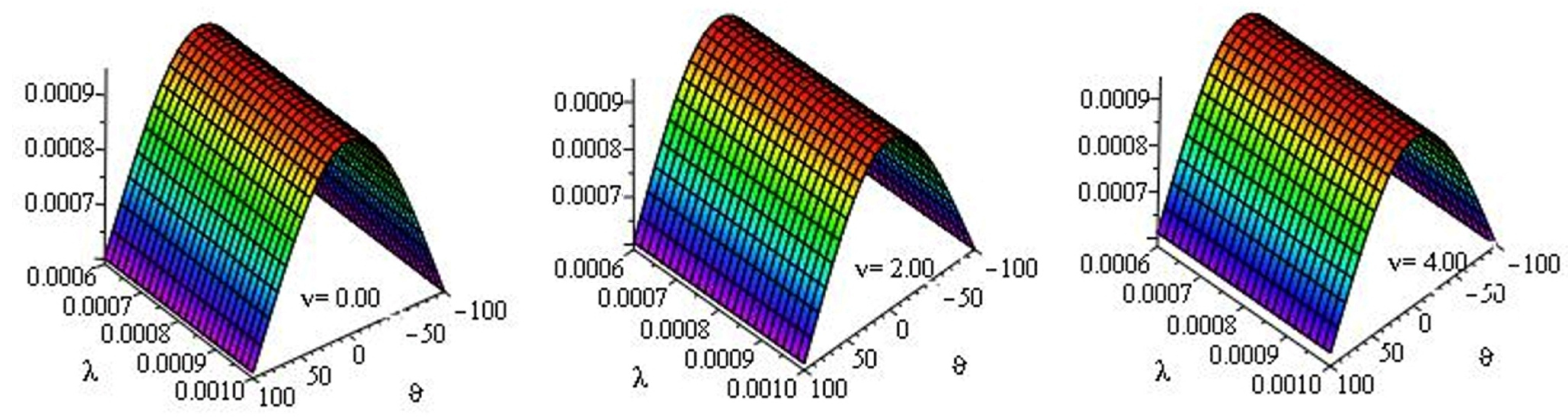
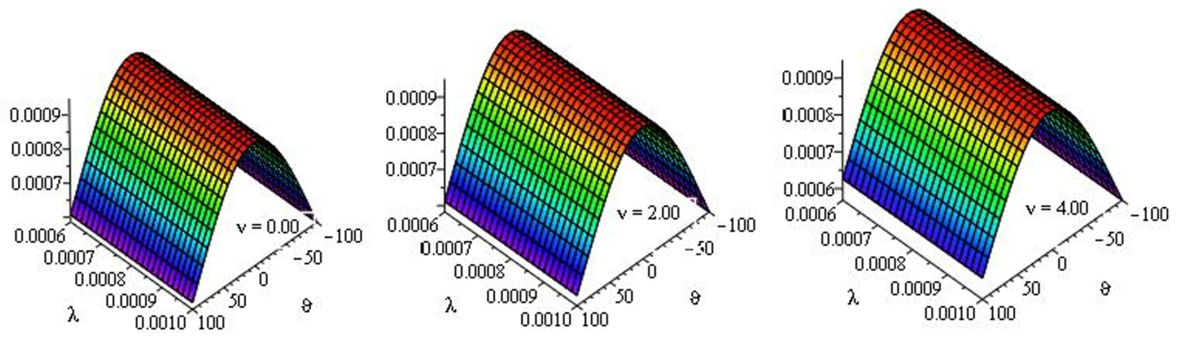
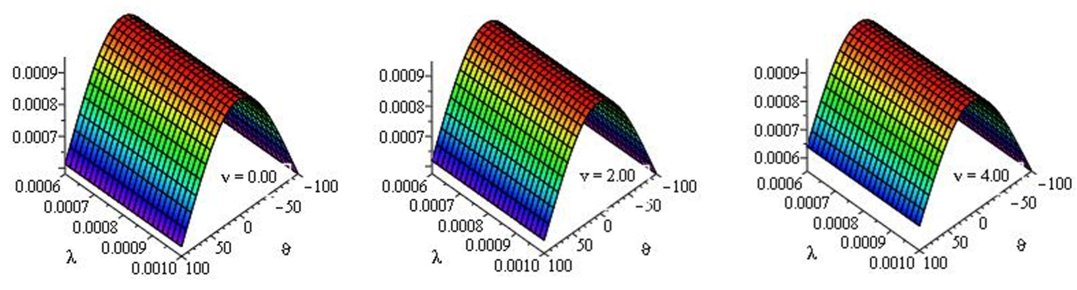
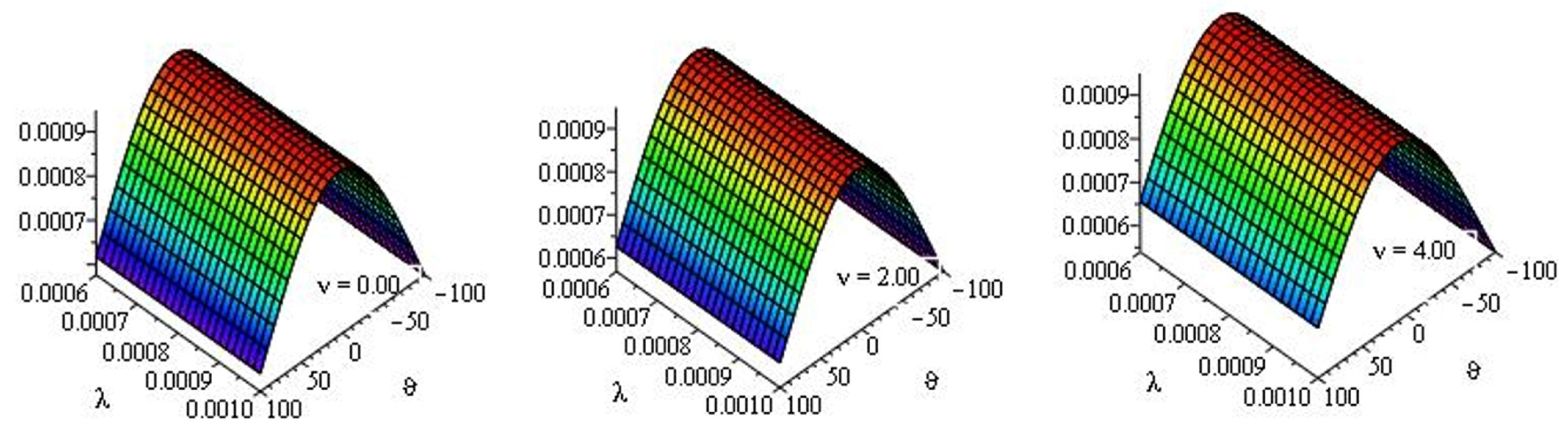
5. Numerical Discussion

Table 1 and Table 2 present the approximate solutions of the MTCFKE (35) for various fractional-order values $\varrho$ and by using numerical imitation. Figure 1, Figure 2, Figure 3, Figure 4 and Figure 5 demonstrate the dynamical behavior of the approximate solutions of the MTCFKE (35). Table 1 presents some comparisons between the absolute error (AE) of the exact solutions of the MTCFKE (35) at $\alpha =0.001$, $\beta =-1$, $\varrho =1$, and $\vartheta =10$ and the approximate solutions of the MTCFKE (35) by using three methods—the LRPSM, the homotopy analysis method (HAM) in [28], and the residual power series method (RPSM) [33]. Table 2 demonstrates the approximate solution of the MTCFKE (35) at $\alpha =0.001$, $\beta =-1$, $\vartheta =10$, and various values of $\varrho$ and $\nu$ by using the LRPSM, and it presents some comparisons between these solutions and the obtained solutions by using the HAM in [28] and the RPSM in [33]. In Figure 1, we present curves of some approximate solutions for the MTCFKE (35) with $\alpha =0.001$, $\beta =-1$, $\nu =0$, $\nu =2$, $\nu =4$, and different values of $\varrho$. For values $\alpha =0.001$, $\beta =-1$, and different values of $\nu$, Figure 2 presents the surface plot of LRPSM solutions for the MTCFKE (35) with $\varrho =1.00$, Figure 3 at $\varrho =0.75$, Figure 4 at $\varrho =0.50$, and Figure 5 at $\varrho =0.25$. Note that the tables and graphs explain the accuracy and applicability of the LRPSM, that is, the figures demonstrate that the symmetry and similarity of the three derivative graphical patterns and the tables with various fractional-order values prove the accuracy of the proposed method with existing techniques.

Table 1. LRPSM’s absolute errors and comparisons with other methods for solving the MTCFKE (35) at $\varrho =1$, $\alpha =0.001$, $\beta =-1$, $\vartheta =10$, and several values of $\nu$.

$\mathit{\nu }$	AE (LRPSM)	AE (NTDM) [32]	AE (RPSM) [33]
$0.0$	0	0	0
$0.1$	$1.41550\times {10}^{-15}$	$1.41553\times {10}^{-15}$	$1.41553\times {10}^{-15}$
$0.2$	$4.68059\times {10}^{-14}$	$4.68063\times {10}^{-14}$	$4.68063\times {10}^{-14}$
$0.3$	$3.63907\times {10}^{-13}$	$3.63910\times {10}^{-13}$	$3.63910\times {10}^{-13}$
$0.4$	$1.56881\times {10}^{-12}$	$1.56886\times {10}^{-12}$	$1.56886\times {10}^{-12}$
$0.5$	$4.89611\times {10}^{-12}$	$4.89617\times {10}^{-12}$	$4.89617\times {10}^{-12}$
$0.6$	$1.24537\times {10}^{-11}$	$1.24542\times {10}^{-11}$	$1.24542\times {10}^{-11}$
$0.7$	$2.75061\times {10}^{-11}$	$2.75069\times {10}^{-11}$	$2.75069\times {10}^{-11}$
$0.8$	$5.47822\times {10}^{-11}$	$5.47829\times {10}^{-11}$	$5.47829\times {10}^{-11}$
$0.9$	$1.00802\times {10}^{-10}$	$1.00810\times {10}^{-10}$	$1.00810\times {10}^{-10}$
$1.0$	$1.74273\times {10}^{-10}$	$1.74280\times {10}^{-10}$	$1.74280\times {10}^{-10}$

Table 2. Comparisons of the LRPSM, NTDM, and HAM for some approximate solutions of the MTCFKE at $\alpha =0.001$, $\beta =-1$, $\varrho =0.25$, and $\varrho =0.5$ with several values of $\vartheta$ and $\nu$.

			$\mathit{\varrho }=0.25$			$\mathit{\varrho }=0.50$
$\mathbf{\nu }$	$\mathbf{\vartheta }$	LRPSM	NTDM [32]	HAM [28]	LRPSM	NTDM [32]	HAM [28]
20	$0.2$	$9.2994\times {10}^{-4}$	$9.2996\times {10}^{-4}$	$9.299\times {10}^{-4}$	$9.2992\times {10}^{-4}$	$9.2996\times {10}^{-4}$	$9.299\times {10}^{-4}$
	$0.4$	$9.2994\times {10}^{-4}$	$9.2996\times {10}^{-4}$	$9.299\times {10}^{-4}$	$9.2992\times {10}^{-4}$	$9.2996\times {10}^{-4}$	$9.299\times {10}^{-4}$
	$0.6$	$9.2994\times {10}^{-4}$	$9.2996\times {10}^{-4}$	$9.299\times {10}^{-4}$	$9.2992\times {10}^{-4}$	$9.2996\times {10}^{-4}$	$9.299\times {10}^{-4}$
	$0.8$	$9.2994\times {10}^{-4}$	$9.2996\times {10}^{-4}$	$9.299\times {10}^{-4}$	$9.2992\times {10}^{-4}$	$9.2996\times {10}^{-4}$	$9.299\times {10}^{-4}$
	$1.0$	$9.2994\times {10}^{-4}$	$9.2996\times {10}^{-4}$	$9.299\times {10}^{-4}$	$9.2992\times {10}^{-4}$	$9.2996\times {10}^{-4}$	$9.299\times {10}^{-4}$
10	$0.2$	$9.4392\times {10}^{-4}$	$9.4396\times {10}^{-4}$	$9.439\times {10}^{-4}$	$9.4391\times {10}^{-4}$	$9.4396\times {10}^{-4}$	$9.439\times {10}^{-4}$
	$0.4$	$9.4392\times {10}^{-4}$	$9.4396\times {10}^{-4}$	$9.439\times {10}^{-4}$	$9.4391\times {10}^{-4}$	$9.4396\times {10}^{-4}$	$9.439\times {10}^{-4}$
	$0.6$	$9.4392\times {10}^{-4}$	$9.4396\times {10}^{-4}$	$9.439\times {10}^{-4}$	$9.4391\times {10}^{-4}$	$9.4396\times {10}^{-4}$	$9.439\times {10}^{-4}$
	$0.8$	$9.4392\times {10}^{-4}$	$9.4396\times {10}^{-4}$	$9.439\times {10}^{-4}$	$9.4391\times {10}^{-4}$	$9.4396\times {10}^{-4}$	$9.439\times {10}^{-4}$
	$1.0$	$9.4392\times {10}^{-4}$	$9.4396\times {10}^{-4}$	$9.439\times {10}^{-4}$	$9.4391\times {10}^{-4}$	$9.4396\times {10}^{-4}$	$9.439\times {10}^{-4}$
0	$0.2$	$9.4863\times {10}^{-4}$	$9.4868\times {10}^{-4}$	$9.486\times {10}^{-4}$	$9.4862\times {10}^{-4}$	$9.4868\times {10}^{-4}$	$9.486\times {10}^{-4}$
	$0.4$	$9.4863\times {10}^{-4}$	$9.4868\times {10}^{-4}$	$9.486\times {10}^{-4}$	$9.4862\times {10}^{-4}$	$9.4868\times {10}^{-4}$	$9.486\times {10}^{-4}$
	$0.6$	$9.4863\times {10}^{-4}$	$9.4868\times {10}^{-4}$	$9.486\times {10}^{-4}$	$9.4862\times {10}^{-4}$	$9.4868\times {10}^{-4}$	$9.486\times {10}^{-4}$
	$0.8$	$9.4863\times {10}^{-4}$	$9.4868\times {10}^{-4}$	$9.486\times {10}^{-4}$	$9.4862\times {10}^{-4}$	$9.4868\times {10}^{-4}$	$9.486\times {10}^{-4}$
	$1.0$	$9.4863\times {10}^{-4}$	$9.4868\times {10}^{-4}$	$9.486\times {10}^{-4}$	$9.4862\times {10}^{-4}$	$9.4868\times {10}^{-4}$	$9.486\times {10}^{-4}$
$-10$	$0.2$	$9.4392\times {10}^{-4}$	$9.4396\times {10}^{-4}$	$9.439\times {10}^{-4}$	$9.4391\times {10}^{-4}$	$9.4396\times {10}^{-4}$	$9.439\times {10}^{-4}$
	$0.4$	$9.4392\times {10}^{-4}$	$9.4396\times {10}^{-4}$	$9.439\times {10}^{-4}$	$9.4391\times {10}^{-4}$	$9.4396\times {10}^{-4}$	$9.439\times {10}^{-4}$
	$0.6$	$9.4863\times {10}^{-4}$	$9.4868\times {10}^{-4}$	$9.486\times {10}^{-4}$	$9.4862\times {10}^{-4}$	$9.4868\times {10}^{-4}$	$9.486\times {10}^{-4}$
	$0.8$	$9.4392\times {10}^{-4}$	$9.4396\times {10}^{-4}$	$9.439\times {10}^{-4}$	$9.4391\times {10}^{-4}$	$9.4396\times {10}^{-4}$	$9.439\times {10}^{-4}$
	$1.0$	$9.4392\times {10}^{-4}$	$9.4396\times {10}^{-4}$	$9.439\times {10}^{-4}$	$9.4391\times {10}^{-4}$	$9.4396\times {10}^{-4}$	$9.439\times {10}^{-4}$
$-20$	$0.2$	$9.2992\times {10}^{-4}$	$9.2996\times {10}^{-4}$	$9.299\times {10}^{-4}$	$9.2991\times {10}^{-4}$	$9.2996\times {10}^{-4}$	$9.299\times {10}^{-4}$
	$0.4$	$9.2992\times {10}^{-4}$	$9.2996\times {10}^{-4}$	$9.299\times {10}^{-4}$	$9.2991\times {10}^{-4}$	$9.2996\times {10}^{-4}$	$9.299\times {10}^{-4}$
	$0.6$	$9.2992\times {10}^{-4}$	$9.2996\times {10}^{-4}$	$9.299\times {10}^{-4}$	$9.2991\times {10}^{-4}$	$9.2996\times {10}^{-4}$	$9.299\times {10}^{-4}$
	$0.8$	$9.2992\times {10}^{-4}$	$9.2996\times {10}^{-4}$	$9.299\times {10}^{-4}$	$9.2991\times {10}^{-4}$	$9.2996\times {10}^{-4}$	$9.299\times {10}^{-4}$
	$1.0$	$9.2992\times {10}^{-4}$	$9.2996\times {10}^{-4}$	$9.299\times {10}^{-4}$	$9.2991\times {10}^{-4}$	$9.2996\times {10}^{-4}$	$9.299\times {10}^{-4}$

Figure 1. LRPSM solutions for the MTCFKE (35) with $\alpha =0.001$, $\beta =-1$, $\nu =0$, $\nu =2$, $\nu =4$, and several values of $\varrho$.

Figure 2. Surface plot of LRPSM solutions for the MTCFKE (35) with $\alpha =0.001$, $\beta =-1$, $\varrho =1.00$, and several values of $\nu$.

Figure 3. Surface plot of LRPSM solutions for the MTCFKE (35) with $\alpha =0.001$, $\beta =-1$, $\varrho =0.75$, and many values of $\nu$.

Figure 4. Surface plot of approximate solutions for the MTCFKE (35) with $\alpha =0.001$, $\beta =-1$, $\varrho =0.50$, and many values of $\nu$.

Figure 5. Surface plot of LRPSM solutions for the MTCFKE (35) with $\alpha =0.001$, $\beta =-1$, $\varrho =0.25$, and many values of $\nu$.

6. Conclusions

Note that in Table 1 and Table 2 above, we observed that the absolute errors for LRPSM solutions of the MTCFKE (35) are less than the absolute errors for both RPSM [33] and HAM solutions [28], that is, the LRPSM was more efficient in deriving the approximate and exact solutions of the MTCFKE (35). The approximate solutions of MTCFKEs are presented by the LRPSM as the series of the convergent sequence ${⟨h_n⟩}_{n=0}^{\infty }$ and the systematic and efficient nature of the LRPSM provided us with approximate solutions that present good results with numerical simulations. The obtained approximate solutions in this work emphasize the method’s suitability in solving partial differential equations for biological systems, mathematical physics systems, and other scientific fields. That is, the results of this study show the proposed method is a good tool for future verification in the context water wave equations, as demonstrated by the comprehensive analysis, efficacy and reliability of the LRPSM in our comparisons, which are introduced in Table 1 and Table 2 and Figure 1, Figure 2, Figure 3, Figure 4 and Figure 5.

References

- Kawahara, T. Oscillatory solitary waves in dispersive media. J. Phys. Soc. Jpn. 1972, 1, 260–264. [Google Scholar] [CrossRef]
- Kudryashov, N.A. A note on new exact solutions for the Kawahara equation using Exp-function method. J. Comput. Appl. Math. 2010, 12, 3511–3512. [Google Scholar] [CrossRef]
- Lu, J. Analytical approach to Kawahara equation using variational iteration method and homotopy perturbation method. Topol. Methods Nonlinear Anal. 2008, 2, 287–293. [Google Scholar]
- Kaya, D.; Al-Khaled, K. A numerical comparison of a Kawahara equation. Phys. Lett. A 2007, 5–6, 433–439. [Google Scholar] [CrossRef]
- Jakub, V. Symmetries and conservation laws for a generalization of Kawahara equation. J. Geom. Phys. 2020, 150, 103579. [Google Scholar]
- Wazwaz, A.M. New solitary wave solutions to the modified Kawahara equation. Phys. Lett. A 2010, 4–5, 588–592. [Google Scholar] [CrossRef]
- Kurulay, M. Approximate analytic solutions of the modified Kawahara equation with homotopy analysis method. Adv. Differ. Equ. 2012, 2012, 178. [Google Scholar] [CrossRef]
- Jin, L. Application of variational iteration method and homotopy perturbation method to the modified Kawahara equation. Math. Comput. Model Dyn. Syst. 2009, 3–4, 573–578. [Google Scholar] [CrossRef]
- Jabbari, A.; Kheiri, H. New exact traveling wave solutions for the Kawahara and modified Kawahara equations by using modified tanh–coth method. Acta Univ. Apulensis Math. Inform. 2010, 23, 21–38. [Google Scholar]
- Damag, F.H.; Kılıçman, A.; Ibrahim, R. Mixed Solutions of Monotone Iterative Technique for Hybrid Fractional Differential Equations. Lobachevskii J. Math. 2019, 40, 156–165. [Google Scholar] [CrossRef]
- Damag, F.H.; Kılıçman, A.; Dutta, H.; Ibrahim, R. Note on the Lower and Upper Solutions of Hybrid-Type Iterative Fractional Differential Equations. Natl. Acad. Sci. Lett. 2020, 34, 277–281. [Google Scholar] [CrossRef]
- Damag, F.H.; Saif, A.; Kiliçman, A. φ–Hilfer Fractional Cauchy Problems with Almost Sectorial and Lie Bracket Operators in Banach Algebras. Fractal Fract. 2024, 8, 741. [Google Scholar] [CrossRef]
- Shah, K.; Seadawy, A.R.; Arfan, M. Evaluation of one dimensional fuzzy fractional partial differential equations. Alex. Eng. J. 2020, 59, 3347–3353. [Google Scholar] [CrossRef]
- Kilic, S.; Celik, E. Complex solutions to the higher-order nonlinear boussinesq type wave equation transform. Ric. Mat. 2022, 73, 1793–1800. [Google Scholar] [CrossRef]
- Akgul, A.; Cordero, A.; Torregrosa, J.R. A fractional Newton method with 2α-order of convergence and its stability. Appl. Math. Lett. 2019, 98, 344–351. [Google Scholar] [CrossRef]
- Yazgan, T.; Ilhan, E.; Çelik, E.; Bulut, H. On the new hyperbolic wave solutions to Wu-Zhang system models. Opt. Quantum Electron. 2022, 54, 298. [Google Scholar] [CrossRef]
- He, J.H. Variational iteration method a kind of non–linear analytical technique: Some examples. Int. J. Non LinearMech. 1999, 4, 699–708. [Google Scholar] [CrossRef]
- Inc, M.; Akgul, A.; Kilicman, A. Explicit solution of telegraph equation based on reproducing kernel method. J. Funct. Spaces Appl. 2012, 2012, 984682. [Google Scholar] [CrossRef]
- Boutarfa, B.; Akgul, A.; Inc, M. New approach for the Fornberg–Whitham type equations. J. Comput. Appl. Math. 2017, 312, 13–26. [Google Scholar] [CrossRef]
- Akgul, A. A novel method for a fractional derivative with non-local and non-singular kernel. Chaos Solit. Fractals. 2018, 114, 478–482. [Google Scholar] [CrossRef]
- Dhaigude, D.B.; Kiwne, S.B.; Dhaigude, R.M. Monotone iterative scheme for weakly coupled system of finite difference reaction diffusion equations. Commun. Appl. Anal. 2008, 2, 161. [Google Scholar]
- Sontakke, B.R.; Shelke, A.S.; Shaikh, A.S. Solution of non-linear fractional differential equations by variational iteration method and applications. Far East J. Math. Sci. 2019, 1, 113–129. [Google Scholar] [CrossRef]
- He, J.H. Homotopy perturbation technique. Comput. Methods Appl. Mech. Eng. 1999, 3–4, 257–262. [Google Scholar] [CrossRef]
- Tazgan, T.; Çelik, E.; Gulnur, Y.E.L.; Bulut, H. On survey of the some wave solutions of the non-linear Schrödinger equation (NLSE) in infinite water depth. Gazi Univ. J. Sci. 2022, 36, 819–843. [Google Scholar] [CrossRef]
- Rahman, M.U.; Arfan, M.; Shah, Z.; Alzahrani, E. Evolution of fractional mathematical model for drinking under Atangana-Baleanu Caputo derivatives. Phys. Scr. 2021, 96, 115203. [Google Scholar] [CrossRef]
- Seadawy, A.R.; Iqbal, M.; Lu, D. Propagation of kink and anti-kink wave solitons for the nonlinear dampedmodified Korteweg-de Vries equation arising in ion-acoustic wave in an unmagnetized collisional dusty plasma. Phys. Stat. Mech. Appl. 2020, 544, 123560. [Google Scholar] [CrossRef]
- Dhaigude, D.B.; Bhadgaonkar, V.N. A novel approach for fractional Kawahara and modified Kawahara equations using Atangana-Baleanu derivative operator. J. Math. Comput. Sci. 2021, 3, 2792–2813. [Google Scholar]
- Zafar, H.; Ali, A.; Khan, K.; Sadiq, M.N. Analytical solution of time fractional Kawahara and modified Kawahara equations by homotopy analysis method. Int. J. Appl. Math. Comput. Sci. 2022, 8, 94. [Google Scholar] [CrossRef]
- Kaur, L.; Gupta, R.K. Kawahara equation and modified Kawahara equation with time dependent coefficients: Symmetry analysis and generalized-expansion method. Math. Methods Appl. Sci. 2013, 36, 584–600. [Google Scholar] [CrossRef]
- Ak, T.; Karakoc, S.B. A numerical technique based on collocation method for solving modified Kawahara equation. J. Ocean. Eng. Sci. 2018, 3, 67–75. [Google Scholar] [CrossRef]
- Bhatter, S.; Mathur, A.; Kumar, D.; Nisar, K.S.; Singh, J. Fractional modified Kawahara equation with Mittag–Leffler law. Chaos Solitons Fractals 2020, 131, 109508. [Google Scholar] [CrossRef]
- Pavani, K.; Raghavendar, K. An efficient technique to solve time-fractional Kawahara and modified Kawahara equations. Symmetry 2022, 14, 1777. [Google Scholar] [CrossRef]
- Culha Unal, S. Approximate solutions of time fractional Kawahara equation by utilizing the residual power series method. Int. J. Appl. Math. Comput. Sci. 2022, 8, 78. [Google Scholar]
- Rahman, M.U.; Arfan, M.; Deebani, W.; Kumam, P.; Shah, Z. Analysis of time-fractional Kawahara equation under Mittag–Leffler Power Law. Fractals 2022, 30, 2240021. [Google Scholar] [CrossRef]
- Khater, M.M. Exploring the rich solution landscape of the generalized Kawahara equation: Insights from analytical techniques. Eur. Phys. J. Plus 2024, 139, 184. [Google Scholar] [CrossRef]
- Shafee, A.; Alkhezi, Y.; Shah, R. Efficient Solution of Fractional System Partial Differential Equations Using Laplace Residual Power Series Method. Fractal Fract. 2023, 7, 429. [Google Scholar] [CrossRef]
- Albalawi, W.; Shah, R.; Nonlaopon, K.; El-Sherif, L.S.; El-Tantawy, S.A. Laplace Residual Power Series Method for Solving Three-Dimensional Fractional Helmholtz Equations. Symmetry 2023, 15, 194. [Google Scholar] [CrossRef]
- Oqielat, M.A.; Eriqat, T.; Ogilat, O.; El-Ajou, A.; Alhazmi, S.E.; Al-Omari, S. Laplace-residual power series method for solving time-fractional reaction–diffusion model. Fractal Fract. 2023, 7, 309. [Google Scholar] [CrossRef]
- Khresat, H.; El-Ajou, A.; Al-Omari, S.; Alhazmi, S.E.; Oqielat, M.N. Exact and Approximate Solutions for Linear and Nonlinear Partial Differential Equations via Laplace Residual Power Series Method. Axioms 2023, 12, 694. [Google Scholar] [CrossRef]
- Belinskii, E.; Liflyand, E.; Trigub, R. The banach algebra A and its properties. J. Fourier Anal. Appl. 1997, 3, 103–129. [Google Scholar] [CrossRef]
- Damag, F.H.; Kılıçman, A.T.; Al-Arioi, A. On Hybrid Type Nonlinear Fractional Integrodifferential Equations. Mathematics 2020, 8, 984. [Google Scholar] [CrossRef]
- Damag, F.; Kiliçman, A. Biological experiments based on fractional integral equations. J. Phys. Conf. Ser. 2018, 1132, 012023. [Google Scholar] [CrossRef]
- Hanna, J.; Rowland, J. Fourier Series, Transforms, and Boundary Value Problems; John Wiley and Sons: Hoboken, NJ, USA, 1990. [Google Scholar]
Disclaimer/Publisher’s Note: The statements, opinions and data contained in all publications are solely those of the individual author(s) and contributor(s) and not of MDPI and/or the editor(s). MDPI and/or the editor(s) disclaim responsibility for any injury to people or property resulting from any ideas, methods, instructions or products referred to in the content. |
© 2025 by the authors. Licensee MDPI, Basel, Switzerland. This article is an open access article distributed under the terms and conditions of the Creative Commons Attribution (CC BY) license (https://creativecommons.org/licenses/by/4.0/).