A Fast High-Order Compact Difference Scheme for Time-Fractional KS Equation with the Generalized Burgers’ Type Nonlinearity

Abstract

This work integrates the fast Alikhanov method with a compact scheme to solve the time-fractional Kuramoto–Sivashinsky (KS) equation with the generalized Burgers’ type nonlinearity. Initially, the Alikhanov algorithm, designed to handle the Caputo fractional derivative on non-uniform time grids, effectively avoids the initial singularity. Additionally, the combination of the Alikhanov method with the sum-of-exponentials (SOE) technique significantly reduces both computational cost and memory requirements. By discretizing the spatial direction using a compact finite difference method, a fully discrete scheme is developed, achieving fourth-order convergence in the spatial domain. Stability and convergence are analyzed through energy methods. Several numerical examples are provided to validate the theoretical framework, demonstrating that the proposed algorithm is accurate, stable, and efficient.

1. Introduction

The Kuramoto–Sivashinsky (KS) equation belongs to an important class of chaotic partial differential equations that serve as a bridge between the partial differential equation and dynamical system frameworks. Kuramoto [1] originally proposed the KS equation in his study of phase turbulence in reaction–diffusion systems, while Sivashinsky [2] introduced it in his analysis of flame combustion propagation models. The KS equation has a wide range of applications in simulation science and engineering, such as the evolution of the flow of fluid films on inclined planes [3], flame front instability [4], interfacial turbulence [5], etc.

In this paper, we study the time-fractional KS equation with the generalized Burgers’ type nonlinearity:

$$\begin{array}{c}\hfill {}_0{}^{C}D_t^{\alpha }u(x,t)+u^p(x,t)u_x(x,t)-\mu u_{xx}(x,t)+\lambda u_{xxxx}(x,t)=f(x,t),\\ \hfill 0<x<L,0<t\le T,\end{array}$$

(1)

with the initial condition (IC)

$$u(x,0)=u_0\left(x\right),0<x<L,$$

(2)

and the boundary conditions (BCs)

$$\begin{array}{c}u(0,t)=u(L,t)=0,0\le t\le T,\hfill \\ u_{xx}(0,t)=u_{xx}(L,t)=0,0\le t\le T,\hfill \end{array}$$

(3)

where $\mu >0$ is the viscosity coefficient, $p\ge 1$ is a positive integer, perturbation parameters $0<\lambda \le 1$, $L>0, T>0$ are fixed values, and $u_0\left(x\right)$ and $f(x,t)$ are prescribed real functions. The equations are complex, and their combination of fractional-order derivative KS equations and Burgers’ nonlinear terms provides them with greater flexibility to capture the intricate dynamical behaviors observed in various physical systems.

•

When the fourth-order derivative $u_{xxxx}$ and the source term are not included in the equation, Equation (1) transforms into a time-fractional generalized Burgers equation [6] as follows:

$${}_0{}^{C}D_t^{\alpha }u(x,t)+u^p(x,t)u_x(x,t)-\mu u_{xx}(x,t)=0,0<x<L,0<t\le T,$$

(4)

where $u^p{u}_x$ is the generalized Burgers’ type nonlinearity.

•

When $\alpha =1$, $p=1$, Equation (1) is the usual KS equation as follows:

$$u_t(x,t)+u(x,t)u_x(x,t)-\mu u_{xx}(x,t)+u_{xxxx}(x,t)=0,0<x<L,0<t\le T,$$

(5)

and many pioneering studies have been carried out [7,8,9].

•

When $p=1$, Equation (1) is the generalized fractional KS equation [10] as follows:

$${}_0{}^{C}D_t^{\alpha }u(x,t)+u(x,t)u_x(x,t)-\mu u_{xx}(x,t)+u_{xxxx}(x,t)=0,0<x<L,0<t\le T,$$

(6)

In recent years, numerical computational algorithms for solving the time-fractional KS equation have been developed and become imperative. Many numerical methods are already available for studying KS equations, including those of the form presented in Equation (5). Mittal [11] proposed a quintic B-spline collocation method based on the Crank–Nicolson scheme for temporal discretization, aimed at approximating the solution to the KS equation. In [12], a locally discontinuous Galerkin method is implemented to obtain the numerical solution to the KS equation. The implicit–explicit BDF method was developed by Akrivis and Smyrlis [13] for simulating the KS equation.

However, there are few research studies on effective numerical algorithms for solving fractional KS equations. For the fractional KS equation of the type Equation (6), the weak singularity of the solution generated by the fractional derivative presents a difficult problem to solve. At present, the effective method to solve this problem is to use the variable step numerical method, which concentrates more grid points around the weak singularity and employs a sparse grid where the solution changes slowly. Indeed, the $L1$ formula for the construction of piecewise linear interpolation was proposed by Langlands [14], which leads to a temporal convergence order of $1+\gamma$ for $0<\gamma <1$. Since then, the $L1$ formula has been widely used to deal with Caputo fractional derivatives [15,16,17,18,19,20]. Furthermore, for the numerical solution to pure sub-diffusion equations, there are several high-order discrete convolution forms for the approximation of the Caputo fractional-order time derivatives, such as the $L1-2$ scheme [21,22,23] and the $L2-1_{\sigma }$ formula, which is based on linear interpolation on the last subinterval $[t_{k-1},t_k]$ and quadratic polynomial interpolation on the rest of the subintervals $[t_{k-1},t_k]$ (for details, please refer to [24]). These formulas can achieve second-order temporal accuracy for sufficiently smooth solutions.

Due to the advantages of the $L2-1_{\sigma }$ formula, we will study the approximation of the Caputo fractional derivative by the variable time-step Alikhanov formula. Influenced by [25,26], we also give the regularity assumptions on the exact solution u as follows:

$$\begin{array}{ccc}\hfill & {∥{\displaystyle \frac{{\partial }^{k}u}{\partial t^k}}∥}_{H^2(0,L)}\le C\left(1+t^{\sigma -k}\right),\hfill & \hfill \hspace{1em}\hspace{1em}\hspace{1em}\hspace{1em}k=0,1,2,3,\end{array}$$

(7)

$$\begin{array}{cc}\hfill & {∥{}_0{}^{C}D_t^{\alpha }u∥}_{H^6(0,L)}+{∥u∥}_{H^8(0,L)}\le C,\hfill \end{array}$$

(8)

where $0<t\le T$, and $\sigma \in (0,1)\cup (1,2)$ is a regularity parameter. In this paper, we only consider the case of $\lambda =1$.

In order to obtain a more efficient algorithm for solving the problem and avoid the issue of large computational costs caused by the historical dependence of the fractional derivative, one of the most effective methods is the SOE technique [27,28,29], which is applied in approximating the convolution kernel $t^{-\alpha }$ with a uniform absolute error $ϵ$. There have been many research studies on the nonlinear KS equation with a spatial fourth derivative, employing various methods such as the quintic B-spline collocation method [30], cubic Hermite collocation [31], Chebyshev collocation method [10], and Sinc–Galerkin method [32]. The compact difference scheme has good characteristics and high accuracy and is widely used to solve a variety of equations [33,34,35,36,37]. The application of a compact difference scheme to the spatial discretization of fractional KS equations is exactly the starting point of our present work. The theoretical part of the proof makes use of the classical energy method [38,39,40]. Moreover, the main contributions of this work can be summarized as follows:

•

For the complex KS equation, we first apply the non-uniform Alikhanov formula to approximate the Caputo fractional derivative, and then treat the generalized Burgers’ nonlinear term. Then, we combine the second-order time scheme and the SOE technique to establish the fast Alikhanov second-order scheme. This approach improves numerical accuracy and reduces computational costs.

•

The high-order compact difference scheme is proposed for the first time to be applied to the KS equation with the generalized Burgers’ nonlinear term, which can improve the spatial convergence rate to the fourth order.

•

We demonstrate in detail the convergence and stability of the fully discrete scheme by the energy argument. In addition, we provide numerical examples to validate the theoretical analysis and demonstrate the efficiency of the algorithm by comparing fast and non-fast Alikhanov schemes.

The outline of this paper is as follows: In Section 2, we introduce some useful notations and lemmas. Additionally, some properties of compact difference formulas and fast Alikhanov formulas are analyzed. In Section 3, the high-order fast Alikhanov compact difference scheme is constructed. The stability and convergence of a full-discrete scheme are investigated. Numerical examples verify the stability and efficiency of the algorithm and the correctness of the theory in Section 4. The conclusion is summarized in Section 5.

2. Preliminaries

In this section, we first recall some basic formulations and useful lemmas. For ease of exposition and proof, we define some notations. To make our analysis extendable, the conditions and properties of the discrete convolution kernel in the Alikhanov formula are also introduced in this section.

2.1. Properties of Compact Difference Scheme

Let the spatial step size $h:=L/M$, where M is a given positive integer. We denote $x_j=jh(0\le j\le M)$ and ${\overline{\mathcal{U}}}_h:=\left\{u\right|u=(u_0,u_1,\dots ,u_M),0\le j\le M\}$. For any $u,v\in {\overline{\mathcal{U}}}_h$, we denote the following notations:

$$\begin{array}{cc}\hfill & {\nabla }^{+}{u}_{j+1}={\displaystyle \frac{1}{h}}\left(u_{j+1}-u_j\right),{\nabla }^{-}{u}_{j-1}={\displaystyle \frac{1}{h}}\left(u_j-u_{j-1}\right),\hfill \\ \hfill & {\nabla }_h{u}_j={\displaystyle \frac{1}{2h}}\left(u_{j+1}-u_{j-1}\right),{\Delta }_x{u}_j={\displaystyle \frac{u_{j+1}-2u_j+u_{j-1}}{h^2}}.\hfill \end{array}$$

We also need to introduce the subspace of ${\overline{\mathcal{U}}}_h$ as ${\mathcal{U}}_h:=\{u\in {\overline{\mathcal{U}}}_h|u_0=u_M=0\}$, and define the inner product and norm as follows:

$$\begin{array}{cc}\hfill & \langle u,v\rangle =h\sum _{j=1}^{M-1}{u}_j{v}_j,(u,v)=h\sum _{j=1}^M\left({\nabla }^{+}{u}_j\right)\left({\nabla }^{+}{v}_j\right),\hfill \\ \hfill & \parallel u\parallel =\sqrt{\langle u,u\rangle }{,\left|u\right|}_1=\sqrt{(u,u)}{,\parallel u\parallel }_{\infty }=\underset{0\le j\le M}{max}\left|u_j\right|.\hfill \end{array}$$

Furthermore, we denote the following:

$${\mathcal{A}}_1{u}_j:=(1+{\displaystyle \frac{h^2}{6}}{\Delta }_x)u_j,{\mathcal{A}}_2{u}_j:=(1+{\displaystyle \frac{h^2}{12}}{\Delta }_x)u_j.$$

Thus, for the discretization of the second and fourth derivatives of the function $u=u(x,t)$, we have the following formulas:

$$u_x\left(x_j\right)={\mathcal{A}}_1^{-1}{\nabla }_h{U}_j+\mathcal{O}\left(h^4\right),u_{xx}\left(x_j\right)={\mathcal{A}}_2^{-1}{\Delta }_x{U}_j+\mathcal{O}\left(h^4\right).$$

(9)

The following transformation can be advanced for the nonlinear term:

$$u^p{u}_x=v{u}_x={\displaystyle \frac{1}{p+2}}[v{u}_x+{\left(vu\right)}_x],$$

(10)

where $v:=u^p,$ and

$$v_j{\displaystyle \frac{\partial u_j}{\partial x}}+{\displaystyle \frac{\partial u_j{v}_j}{\partial x}}=v_j{\mathcal{A}}_1^{-1}{\nabla }_h{u}_j+{\mathcal{A}}_1^{-1}{\nabla }_h\left(v_j{u}_j\right)+\mathcal{O}\left(h^4\right)=\phi (u_j,v_j)+\mathcal{O}\left(h^4\right).$$

(11)

Lemma 1 

([41]). For any grid functions $u,v\in {\mathcal{U}}_h$, then the following holds:

$$\langle {\nabla }_{h}u,v\rangle =-\langle u,{\nabla }_{h}v\rangle ,\langle {\Delta }_{x}u,v\rangle =-(u,v).$$

Lemma 2 

([41]). For any grid functions $u\in {\mathcal{U}}_h$, then the following holds:

$${\parallel u\parallel }_{\infty }\le {\displaystyle \frac{\sqrt{L}}{2}}{\left|u\right|}_1,\parallel u\parallel \le {\displaystyle \frac{L}{\sqrt{6}}}{\left|u\right|}_1{,\left|u\right|}_1\le {\displaystyle \frac{2}{h}}\parallel u\parallel .$$

Lemma 3 

([42]). For real symmetric positive-definite matrices ${\mathcal{A}}_1^{-1}$, ${\mathcal{A}}_2^{-1}$, and $\omega ,u\in {\mathcal{U}}_h$, we obtain the following:

$$\begin{array}{c}\left({\mathcal{A}}_1^{-1}\omega ,u\right)=\left({\mathcal{V}}_1\omega ,{\mathcal{V}}_{1}u\right)=\left(\omega ,{\mathcal{A}}_1^{-1}u\right),\left({\mathcal{A}}_2^{-1}\omega ,u\right)=\left({\mathcal{V}}_2\omega ,{\mathcal{V}}_{2}u\right)=\left(\omega ,{\mathcal{A}}_2^{-1}u\right),\hfill \end{array}$$

where ${\mathcal{V}}_1$ and ${\mathcal{V}}_2$ are upper triangular matrices, which can be obtained by the Cholesky factorization of ${\mathcal{A}}_1^{-1}$ and ${\mathcal{A}}_2^{-1}$, namely, ${\mathcal{A}}_1^{-1}={\left({\mathcal{V}}_1\right)}^T{\mathcal{V}}_1$, ${\mathcal{A}}_2^{-1}={\left({\mathcal{V}}_2\right)}^T{\mathcal{V}}_2$.

Proof. 

The proof of the theorem can be referred to in ([42], Lemma 2.1c). □

Lemma 4 

([43]). Let $\omega ,u\in {\mathcal{U}}_h$, then we can obtain the following:

$$\begin{array}{c}\left({\mathcal{A}}_1^{-1}{\nabla }_h\omega ,u\right)=\left({\nabla }_h{\mathcal{A}}_1^{-1}\omega ,u\right)=-\left({\mathcal{A}}_1^{-1}\omega ,{\nabla }_{h}u\right)=-\left(\omega ,{\mathcal{A}}_1^{-1}{\nabla }_{h}u\right),\hfill \\ \left({\mathcal{A}}_2^{-1}{\Delta }_x\omega ,u\right)=\left({\Delta }_x{\mathcal{A}}_2^{-1}\omega ,u\right)=-\left({\nabla }^{+}{\mathcal{A}}_2^{-1}\omega ,{\nabla }^{+}u\right)=-\left({\mathcal{A}}_2^{-1}{\nabla }^{+}\omega ,{\nabla }^{+}u\right).\hfill \end{array}$$

Lemma 5. 

Let $u,v\in {\mathcal{U}}_h$, we arrive at

$$〈\phi (u,v),u〉=0.$$

Proof. 

For $u,v\in {\mathcal{U}}_h$, using Lemmas 1 and 4, we can obtain the following:

$$\begin{array}{cc}\hfill 〈\phi (u,v),u〉& =〈v_j{\mathcal{A}}_1^{-1}{\nabla }_h{u}_j+{\mathcal{A}}_1^{-1}{\nabla }_h\left(v_j{u}_j\right),u_j〉\hfill \\ \hfill & =〈v_j{\mathcal{A}}_1^{-1}{\nabla }_h{u}_j,u_j〉+〈{\mathcal{A}}_1^{-1}{\nabla }_h\left(v_j{u}_j\right),u_j〉,\hfill \\ \hfill & =〈{\mathcal{A}}_1^{-1}{\nabla }_h{u}_j,v_j{u}_j〉-〈v_j{u}_j,{\mathcal{A}}_1^{-1}{\nabla }_h{u}_j〉,\hfill \\ \hfill & =0.\hfill \end{array}$$

□

Lemma 6 

([43]). For real symmetric positive-definite matrices ${\mathcal{A}}_1^{-1}$, ${\mathcal{A}}_2^{-1}$, and $\omega \in {\mathcal{U}}_h$, we obtain the following:

$$\begin{array}{c}{\parallel \omega \parallel }^2\le \left({\mathcal{A}}_1^{-1}\omega ,\omega \right)= \parallel {\mathcal{V}}_1{\omega \parallel }^2\le {3\parallel \omega \parallel }^2{,\parallel \omega \parallel }^2\le \left({\mathcal{A}}_2^{-1}\omega ,\omega \right)= \parallel {\mathcal{V}}_2{\omega \parallel }^2\le {\displaystyle \frac{3}{2}}{\parallel \omega \parallel }^2.\hfill \end{array}$$

2.2. Properties of the Fast Alikhanov Scheme

In order to construct the fast Alikhanov scheme, we first consider the time levels $0=t_0<t_1<t_2<\cdots <t_N=T$, where N is a given positive integer. We define the nth step size ${\tau }_n:=t_n-t_{n-1}$ for $1\le n\le N$, the maximum step size $\tau :=\underset{0\le n\le N}{max}{\tau }_n$. We set the time level $t_{n-\theta }:=\theta t_{n-1}+(1-\theta )t_n$ with a fixed parameter $\theta =\alpha /2$. It is necessary to set the local step-size ratios:

$${\rho }_n:={\displaystyle \frac{{\tau }_n}{{\tau }_{n+1}}}\mathrm{for}1\le n\le N-1\mathrm{and}\rho :=\underset{1\le n\le N-1}{max}{\rho }_n.$$

For any time sequence ${\left(v^n\right)}_{n=0}^N$, we define ${\nabla }_{\tau }{v}^n:=v^n-v^{n-1}$ and the interpolated value $v^{n-\theta }:=\theta v^{n-1}+(1-\theta )v^n$. Thus, it is advisable to denote ${\mathrm{\Pi }}_{1,k}u$ as the linear interpolant function of a function, u, with respect to $t_{k-1},t_k$, and to denote the quadratic interpolant of u with respect to $t_{k-1},t_k$ and $t_{k+1}$ as ${\mathrm{\Pi }}_{2,k}u$, respectively. Recalling the definition of ${\nabla }_{\tau }{u}^k$, it follows that for $k\ge 1$, we have the following:

$$\begin{array}{cc}\hfill {\left({\mathrm{\Pi }}_{1,k}u\right)}^{\prime }\left(t\right)& ={\displaystyle \frac{{\nabla }_{\tau }{u}^k}{{\tau }_k}},\hfill \\ \hfill {\left({\mathrm{\Pi }}_{2,k}u\right)}^{\prime }\left(t\right)& ={\displaystyle \frac{{\nabla }_{\tau }{u}^k}{{\tau }_k}}+{\displaystyle \frac{2\left(t-t_{k-1/2}\right)}{{\tau }_k\left({\tau }_k+{\tau }_{k+1}\right)}}\left({\rho }_k{\nabla }_{\tau }{u}^{k+1}-{\nabla }_{\tau }{u}^k\right).\hfill \end{array}$$

Next, the Caputo fractional derivative can be approximated by the defined interpolant polynomial at $t_{n-\theta }$ to obtain the Alikhanov approximation:

$$\begin{array}{cc}\hfill {\left(D_{\tau }^{\alpha }u\right)}^{n-\theta }& :={\int }_{t_{n-1}}^{t_{n-\theta }}{\omega }_{1-\alpha }(t_{n-\theta }-s){\left({\mathrm{\Pi }}_{1,n}u\right)}^{\prime }\left(s\right)\mathrm{d}s+\sum _{k=1}^{n-1}{\int }_{t_{k-1}}^{t_k}{\omega }_{1-\alpha }(t_{n-\theta }-s){\left({\mathrm{\Pi }}_{2,k}u\right)}^{\prime }\left(s\right)\mathrm{d}s\hfill \\ \hfill & =a_0^{\left(n\right)}{\nabla }_{\tau }{u}^n+\sum _{k=1}^{n-1}\left(a_{n-k}^{\left(n\right)}{\nabla }_{\tau }{u}^k+{\rho }_k{b}_{n-k}^{\left(n\right)}{\nabla }_{\tau }{u}^{k+1}-b_{n-k}^{\left(n\right)}{\nabla }_{\tau }{u}^k\right),\hfill \\ \hfill & =\sum _{k=1}^n{A}_{n-k}^{(\alpha ,n)}{\nabla }_{\tau }{v}^k,\hfill \end{array}$$

(12)

we have $A_0^{\left(1\right)}:=a_0^{\left(1\right)}$ if $n=1$, and for $n\ge 2$,

$$\begin{array}{cc}\hfill & A_{n-k}^{\left(n\right)}:=\left\{\begin{array}{cc}{a}_0^{\left(n\right)}+{\rho }_{n-1}{b}_1^{\left(n\right)},\hfill & k=n,\hfill \\ a_{n-k}^{\left(n\right)}+{\rho }_{k-1}{b}_{n-k+1}^{\left(n\right)}-b_{n-k}^{\left(n\right)},\hfill & 2\le k\le n-1,\hfill \\ a_{n-1}^{\left(n\right)}-b_{n-1}^{\left(n\right)},\hfill & k=1.\hfill \end{array}\right.\hfill \end{array}$$

(13)

Here, $A_{n-k}^{\left(n\right)}$ is the discrete convolution kernel of the Alikhanov formula; next, the SOE technique is applied to derive the discrete convolution kernel of the fast Alikhanov formula.

Lemma 7 

([27]). (SOE) Let $\alpha \in (0,1)$, $ϵ\ll 1$, and $\Delta t>0$. Assume there exists a positive integer $N_q$, and positive quadrature nodes $s^l$ and ${\varpi }^l>0$$(1\le l\le N_q)$, such that we have the following:

$$\left|{\omega }_{1-\alpha }\left(t\right)-\sum _{l=1}^{N_q}{\varpi }^l{e}^{-s^{l}t}\right|\le ϵ,t\in [\Delta t,T],$$

and the quadrature node number $N_q$ satisfies

$$N_q=O\left(log{\displaystyle \frac{1}{ϵ}}\left(loglog{\displaystyle \frac{1}{ϵ}}+log{\displaystyle \frac{T}{\Delta t}}\right)+log{\displaystyle \frac{1}{\Delta t}}\left(loglog{\displaystyle \frac{1}{ϵ}}+log{\displaystyle \frac{1}{\Delta t}}\right)\right).$$

Now, the fractional derivative can be approximated in combination with the SOE technique in Lemma 7 at the time point $t_{n-\theta }$ for $1\le n\le N$

$$\begin{array}{cc}\hfill {}_0{}^{C}D_f^{\alpha }u\left(t_{n-\theta }\right)& \approx {\int }_{t_{n-1}}^{t_{n-\theta }}{\omega }_{1-\alpha }(t_{n-\theta }-s){\left({\mathrm{\Pi }}_{1,n}u\right)}^{\prime }\left(s\right)\mathrm{d}s+\sum _{k=1}^{n-1}{\int }_{t_{k-1}}^{t_k}\sum _{l=1}^{N_q}{\varpi }^l{e}^{-s^l\left(t_{n-\theta }-s\right)}{u}^{\prime }\left(s\right)\mathrm{d}s\hfill \\ \hfill & ={\widehat{\mathbf{a}}}_0^{\left(n\right)}{\nabla }_{\tau }{u}^n+\sum _{k=1}^{n-1}\left({\widehat{\mathbf{a}}}_{n-k}^{\left(n\right)}{\nabla }_{\tau }{u}^k+{\rho }_k{\widehat{\mathbf{b}}}_{n-k}^{\left(n\right)}{\nabla }_{\tau }{u}^{k+1}-{\widehat{\mathbf{b}}}_{n-k}^{\left(n\right)}{\nabla }_{\tau }{u}^k\right)\hfill \\ \hfill & =\sum _{k=1}^n{\widehat{\mathbf{A}}}_{n-k}^{\left(n\right)}{\nabla }_{\tau }{u}^k,\hfill \end{array}$$

(14)

where coefficients ${\widehat{\mathbf{a}}}_{n-k}^{\left(n\right)}$ and ${\widehat{\mathbf{b}}}_{n-k}^{\left(n\right)}$ are defined by the following:

$${\widehat{\mathbf{a}}}_0^{\left(n\right)}:=a_0^{\left(n\right)},{\widehat{\mathbf{a}}}_{n-k}^{\left(n\right)}:={\displaystyle \frac{1}{{\tau }_k}}{\int }_{t_{k-1}}^{t_k}\sum _{l=1}^{N_q}{\varpi }^l{e}^{-s^l\left(t_{n-\theta }-s\right)}\mathrm{d}s,1\le k\le n-1,$$

$${\widehat{\mathbf{b}}}_{n-k}^{\left(n\right)}:={\displaystyle \frac{2}{{\tau }_k\left({\tau }_k+{\tau }_{k+1}\right)}}{\int }_{t_{k-1}}^{t_k}\sum _{l=1}^{N_q}{\varpi }^l{e}^{-s^l\left(t_{n-\theta }-s\right)}{e}^{-s^l\left(t_{k+1-\theta }-s\right)}(s-t_{k-{\displaystyle \frac{1}{2}}})\mathrm{d}s,1\le k\le n-1.$$

We reformulate the discrete convolution kernel ${\widehat{\mathbf{A}}}_{n-k}^{\left(n\right)}$ as follows: ${\widehat{\mathbf{A}}}_0^{\left(1\right)}:=a_0^{\left(1\right)}$ if $n=1$ and for $n\ge 2$

$${\widehat{\mathbf{A}}}_{n-k}^{\left(n\right)}:=\left\{\begin{array}{cc}{\widehat{\mathbf{a}}}_0^{\left(n\right)}+{\rho }_{n-1}{\widehat{\mathbf{b}}}_1^{\left(n\right)},\hfill & \mathrm{for}k=n,\hfill \\ {\widehat{\mathbf{a}}}_{n-k}^{\left(n\right)}+{\rho }_{k-1}{\widehat{\mathbf{b}}}_{n-k+1}^{\left(n\right)}-{\widehat{\mathbf{b}}}_{n-k}^{\left(n\right)},\hfill & \mathrm{for}2\le k\le n-1,\hfill \\ {\widehat{\mathbf{a}}}_{n-1}^{\left(n\right)}-{\widehat{\mathbf{b}}}_{n-1}^{\left(n\right)},\hfill & \mathrm{for}k=1.\hfill \end{array}\right.$$

(15)

In order to effectively assess some necessary properties of the discrete convolution kernel ${\widehat{\mathbf{A}}}_{n-k}^{\left(n\right)}$, the time step needs to satisfy the following two conditions:

• M1. The maximum time-step ratio is $\rho =7/4$.
• M2. There exists a positive constant $C_{\gamma }$, such that ${\tau }_k\le C_{\gamma }\tau min\{1,t_k^{1-1/\gamma }\}$ for $1\le k\le N$, with $t_k\le C_{\gamma }{t}_{k-1}$ and ${\tau }_k/t_k\le C_{\gamma }{\tau }_{k-1}/t_{k-1}$ for $2\le k\le N$.

Lemma 8 

([27]). Assume that the tolerance error ϵ of the SOE approximation satisfies

$$ϵ\le min\left\{{\displaystyle \frac{{\alpha }_p}{2(1-{\alpha }_p)}}{\omega }_{1-{\alpha }_p}\left(T\right),{\displaystyle \frac{1}{26}}{\omega }_{1-{\alpha }_p}\left(T\right)\right\},$$

then the discrete kernel ${\widehat{\mathbf{A}}}_{n-k}^{\left(n\right)}$ satisfies the following:

(I)

${\widehat{\mathbf{A}}}_{n-k}^{\left(n\right)}$ are bounded, ${\widehat{\mathbf{A}}}_{n-k}^{\left(n\right)}\le {\displaystyle \frac{2}{{\tau }_n}}{\omega }_{2-{\alpha }_p}\left({\tau }_n\right)$ and

$${\widehat{\mathbf{A}}}_{n-k}^{\left(n\right)}\ge {\displaystyle \frac{1}{2{\tau }_k}}{\int }_{t_{k-1}}^{t_k}{\omega }_{1-\alpha }(t_n-s)\mathrm{d}s,1\le k\le n;$$

(II)

${\widehat{\mathbf{A}}}_{n-k}^{\left(n\right)}$ are monotone, and

$${\widehat{\mathbf{A}}}_{n-k-1}^{\left(n\right)}-{\widehat{\mathbf{A}}}_{n-k}^{\left(n\right)}\ge (1+{\rho }_k)\left({\displaystyle \frac{1}{5{\rho }_k}}+1\right)b_{n-k}^{\left(n\right)},1\le k\le n-1;$$

(III)

${\widehat{\mathbf{A}}}_0^{\left(n\right)}-{\widehat{\mathbf{A}}}_1^{\left(n\right)}>\theta \left(2{\widehat{\mathbf{A}}}_0^{\left(n\right)}-{\widehat{\mathbf{A}}}_1^{\left(n\right)}\right)$ for $n\ge 2.$

In this case, for the later analysis of global consistency, we introduce the complementary discrete convolution kernels $P_{n-k}^{\left(n\right)}$ of ${\widehat{\mathbf{A}}}_{n-k}^{\left(n\right)}$ that satisfy

$$\sum _{i=k}^n{P}_{n-i}^{\left(n\right)}{\widehat{\mathbf{A}}}_{i-k}^{\left(i\right)}\equiv 1.$$

(16)

which yields the following recursive formulas:

$$P_0^{\left(n\right)}:={\displaystyle \frac{1}{{\widehat{\mathbf{A}}}_0^{\left(n\right)}}},P_i^{\left(n\right)}:={\displaystyle \frac{1}{{\widehat{\mathbf{A}}}_0^{\left(i\right)}}}\sum _{k=i+1}^n\left({\widehat{\mathbf{A}}}_{k-i-1}^{\left(k\right)}-{\widehat{\mathbf{A}}}_{k-i}^{\left(k\right)}\right)P_k^{\left(n\right)},1\le i\le n-1.$$

In fact, according to Lemma 8, the complementary discrete kernels are non-negative and satisfy the following:

$$\sum _{i=1}^n{P}_{n-i}^{\left(n\right)}{\omega }_{1+(m-1)\alpha }\left(t_i\right)\le {\pi }_A{\omega }_{1+m\alpha }\left(t_n\right),m=0,1,1\le n\le N.$$

(17)

Lemma 9 

([44]). Let ${\lambda }_s$ be nonnegative constants with $0<{\sum }_{s=0}^n{\lambda }_s\le \mathrm{\Lambda }$ for $n\ge 1$, where Λ is some positive constant independent of n. Suppose that the nonnegative sequences ${\xi }_n$ and ${\eta }_n$ are bounded, and the nonnegative grid function $\{v_n\mid n\ge 0\}$ satisfies the following:

$$\sum _{k=1}^n{A}_{n-k}^{\left(n\right)}{\nabla }_{\tau }{\left(v^k\right)}^2\le \sum _{s=1}^n{\lambda }_{n-s}{\left(v^{s,{\theta }_1}\right)}^2+{\xi }^n{v}^{n,{\theta }_2}+{\left({\eta }^n\right)}^2,n\ge 1,$$

(18)

where for $i=1,2$ and each n, we set $v^{n,{\theta }_1}:={\theta }_i{v}^{n-1}+(1-{\theta }_i)v^n$ for some constant ${\theta }_i\in [0,1]$. If the nonuniform grid satisfies the maximum time-step criterion ${\tau }_N\le {\left[{\displaystyle \frac{11}{2}}\mathrm{\Gamma }(2-\alpha )\mathrm{\Lambda }\right]}^{-1/\alpha }$, then we have the following:

$$v^n\le 2E_{\alpha }\left({\displaystyle \frac{11}{2}}\mathrm{\Lambda }{t}_n^{\alpha }\right)\left[v^0+\underset{1\le k\le n}{max}\sum _{j=1}^k{P}_{k-j}^{\left(k\right)}({\xi }^j+{\eta }^j)+\underset{1\le j\le n}{max}{\eta }^j\right],1\le n\le N,$$

where $E_{\alpha }\left(z\right):={\displaystyle \sum _{k=0}^{\infty }}{z}^k/\mathrm{\Gamma }(1+k\alpha )$, and $E_{\alpha }(·)$ represents the Mittag–Leffler function.

Lemma 10 

([45]). Under the condition M1 and Lemma 8, the fast Alikhanov Formula (14) satisfies the following:

$$〈{\left({\mathcal{D}}_{\tau }^{\alpha }v\right)}^{n-\theta },v^{n-\theta }〉\ge {\displaystyle \frac{1}{2}}\sum _{k=1}^n{A}_{n-k}^{\left(n\right)}{\nabla }_{\tau }(\parallel v^k{\parallel }^2),1\le n\le N.$$

3. Establishment and Analysis of Compact Scheme

In this section, we shall derive the second-order fast compact difference scheme for problems (1)–(3). After that, the convergence and stability of the fast compact difference algorithm are rigorously proved.

3.1. Numerical Scheme

First, combined with (11), the temporal direction of Equation (1) at the grid points $(x_j,t_{n-\theta })$ is discretized by the fast nonuniform Alikhanov Formula (14) and the spatial direction is discretized by the compact difference Formula (9), where we obtain the following:

$$\{\begin{array}{}\hfill \hspace{1em}& {\left({\mathcal{D}}_f^{\alpha }{U}_j\right)}^{n-\theta }+{\displaystyle \frac{1}{p+2}}\phi (V_j^{n-\theta },U_j^{n-\theta })-\mu {\mathcal{A}}_2^{-1}{\Delta }_x{U}_j^{n-\theta }+{\mathcal{A}}_2^{-1}{\Delta }_x{W}_j^{n-\theta }=f_j^{n-\theta }+{\mathrm{\Lambda }}_j^{n-\theta },\hfill \hfill \mathrm{(19)}& 1\le j\le M-1,1\le n\le N,\hfill \hfill \mathrm{(20)}& V_j^n={\left(U_j^n\right)}^p,0\le j\le M,0\le n\le N,\hfill \hfill \mathrm{(21)}& W_j^{n-\theta }={\Delta }_x{U}_j^{n-\theta }+R_3^{n-\theta },0\le j\le M,0\le n\le N,\hfill \end{array}$$

where ${\mathrm{\Lambda }}_j^{n-\theta }$ and $R_3^{n-\theta }$ denote the truncation errors.

Omitting the small terms ${\mathrm{\Lambda }}_j^{n-\theta }$ and $R_3^{n-\theta }$ in (19), we replace the functions $U_j^n$, $W_j^n$, and $V_j^n$ with their numerical approximations $u_j^n$, ${\omega }_j^n$, and $v_j^n$, respectively. Meanwhile, combining IC (2) and BC (3), we can obtain the fully discrete difference scheme:

$$\{\begin{array}{}\hfill \mathrm{(22)}& {\left({\mathcal{D}}_f^{\alpha }{u}_j\right)}^{n-\theta }+{\displaystyle \frac{1}{p+2}}\phi (v_j^{n-\theta },u_j^{n-\theta })-\mu {\mathcal{A}}_2^{-1}{\Delta }_x{u}_j^{n-\theta }+{\mathcal{A}}_2^{-1}{\Delta }_x{\omega }_j^{n-\theta }=f_j^{n-\theta },\hfill \hfill \hspace{1em}& 1\le j\le M-1,1\le n\le N,\hfill \hfill \mathrm{(23)}& v_j^n={\left(u_j^n\right)}^p,0\le j\le M,0\le n\le N,\hfill \hfill \mathrm{(24)}& {\omega }_j^{n-\theta }={\Delta }_x{u}_j^{n-\theta },0\le j\le M,0\le n\le N,\hfill \hfill \mathrm{(25)}& u_j^0=u_0\left(x_j\right),1\le j\le M-1,\hfill \hfill \mathrm{(26)}& u_0^n=u_M^n={\omega }_0^n={\omega }_M^n=0,0\le n\le N.\hfill \end{array}$$

In what follows, the stability and convergence analysis of the above fully discrete schemes (22)–(26) are carried out by the energy method.

3.2. Stability

Here, we present the stability result as follows:

Theorem 1. 

Suppose that ${\left\{u^n\right\}}_{n=0}^N$ is the solution to (22)–(26), and under the conditions of Lemma 8 and M2, then we have the following:

$$\parallel u^n\parallel \le \parallel u_0\parallel + {\displaystyle \frac{11}{2}}\mathrm{\Gamma }(1-\alpha )\underset{1\le k\le n}{max}{t}_k^{\alpha }\parallel f^{k-\theta }\parallel .$$

Proof. 

Taking an inner product of (22) with $u^{n-\theta }$, we obtain the following:

$$\begin{array}{cc}\hfill 〈{\left({\mathcal{D}}_f^{\alpha }u\right)}^{n-\theta },u^{n-\theta }〉+{\displaystyle \frac{1}{p+2}}〈\phi (v^{n-\theta },u^{n-\theta }),u^{n-\theta }〉& -\mu 〈{\mathcal{A}}_2^{-1}{\Delta }_x{u}^{n-\theta },u^{n-\theta }〉+〈{\mathcal{A}}_2^{-1}{\Delta }_x{\omega }^{n-\theta },u^{n-\theta }〉\hfill \\ \hfill & =〈f^{n-\theta },u^{n-\theta }〉.\hfill \end{array}$$

(27)

By Lemmas 5 and 10, we have the following:

$$〈{\left({\mathcal{D}}_f^{\alpha }u\right)}^{n-\theta },u^{n-\theta }〉\ge {\displaystyle \frac{1}{2}}\sum _{k=1}^n{A}_{n-k}^{\left(n\right)}{\nabla }_{\tau }(\parallel u^k{\parallel }^2),$$

(28)

$${\displaystyle \frac{1}{p+2}}〈\phi (v^{n-\theta },u^{n-\theta }),u^{n-\theta }〉=0,$$

(29)

and

$$-\mu 〈{\mathcal{A}}_2^{-1}{\Delta }_x{u}^{n-\theta },u^{n-\theta }〉=\mu 〈{\mathcal{A}}_2^{-1}{\nabla }^{+}{u}^{n-\theta },{\nabla }^{+}{u}^{n-\theta }〉\ge \mu \mid u^{n-\theta }{\mid }_1^2,$$

(30)

$$〈{\mathcal{A}}_2^{-1}{\Delta }_x{\omega }^{n-\theta },u^{n-\theta }〉=〈{\mathcal{A}}_2^{-1}{\omega }^{n-\theta },{\Delta }_x{u}^{n-\theta }〉=〈{\mathcal{A}}_2^{-1}{\omega }^{n-\theta },{\omega }^{n-\theta }〉\ge 0.$$

(31)

Under the relations (28)–(31), we have the following:

$$\sum _{k=1}^n{A}_{n-k}^{\left(n\right)}{\nabla }_{\tau }(\parallel u^k{\parallel }^2) \le 2\parallel f^{n-\theta }\parallel \parallel u^{n-\theta }\parallel .$$

Taking ${\lambda }_s=0$ for $s\ge 0$, ${\eta }^n=0$ and ${\xi }^n=2\parallel f^{n-\theta }\parallel$ for $n\ge 1$ in Lemma 9 and ${\pi }_A={\displaystyle \frac{11}{4}}$ in Lemma 8, it is easy to obtain

$$\parallel u^n\parallel \le \parallel u_0\parallel +\underset{1\le k\le n}{max}\sum _{i=1}^{k}2P_{k-i}^{\left(k\right)}\parallel f^{k-\theta }\parallel \le \parallel u_0\parallel + 2{\pi }_A\mathrm{\Gamma }(1-\alpha )\underset{1\le k\le n}{max}{t}_k^{\alpha }\parallel f^{k-\theta }\parallel .$$

Consequently, we infer the following:

$$\parallel u^n\parallel \le \parallel u_0\parallel + {\displaystyle \frac{11}{2}}\mathrm{\Gamma }(1-\alpha )\underset{1\le k\le n}{max}{t}_k^{\alpha }\parallel f^{k-\theta }\parallel .$$

□

3.3. Convergence

Before analyzing the convergence of the fast Alikhanov schemes (22)–(26), we first analyze the truncation errors ${\mathrm{\Lambda }}_j^{n-\theta }$ and ${\left(R_3\right)}_j^{n-\theta }$. In fact, ${\mathrm{\Lambda }}_j^{n-\theta }$ is composed of the following four parts:

$${\mathrm{\Lambda }}_j^{n-\theta }:={\left(R_{t1}\right)}_j^{n-\theta }+{\left(R_{t2}\right)}_j^{n-\theta }+{\left(R_3\right)}_j^{n-\theta }+{\left(R_s\right)}_j^{n-\theta },1\le j\le M-1,1\le n\le N,$$

where ${\left(R_s\right)}_j^{n-\theta }$ means that the error is caused by approximating space derivatives; it can easily be seen that ${\left(R_s\right)}_j^{n-\theta }=\mathcal{O}\left(h^4\right)$ from (9) and (11). Moreover, we have the following:

$$\begin{array}{cc}\hfill & {\left(R_{t1}\right)}_j^{n-\theta }:={\left({\mathcal{D}}_f^{\alpha }{u}_j\right)}^{n-\theta }-{}_0{}^{C}D_t^{\alpha }u(x_j,t_{n-\theta }),\hfill \\ \hfill & {\left(R_{t2}\right)}_j^{n-\theta }:=-{\displaystyle \frac{1}{p+2}}\phi ({\left(R_v\right)}_j^{n-\theta },{\left(R_u\right)}_j^{n-\theta })+\mu {\mathcal{A}}_2^{-1}{\Delta }_x{\left(R_u\right)}_j^{n-\theta }-{\mathcal{A}}_2^{-1}{\Delta }_x{\left(R_{\omega }\right)}_j^{n-\theta },\hfill \end{array}$$

where ${\left(R_u\right)}_j^{n-\theta }$, ${\left(R_v\right)}_j^{n-\theta }$ and ${\left(R_{\omega }\right)}_j^{n-\theta }$ denote the errors of the weighted time approximation at $t_{n-\theta }$, namely, we have the following:

$$\begin{array}{cc}\hfill {\left(R_u\right)}_j^{n-\theta }& :=u(x_j,t_{n-\theta })-[\theta U_j^{n-1}+(1-\theta )U_j^n],\hfill \\ \hfill {\left(R_v\right)}_j^{n-\theta }& :=v(x_j,t_{n-\theta })-[\theta V_j^{n-1}+(1-\theta )V_j^n],\hfill \\ \hfill {\left(R_{\omega }\right)}_j^{n-\theta }& :=\omega (x_j,t_{n-\theta })-[\theta W_j^{n-1}+(1-\theta )W_j^n].\hfill \end{array}$$

Based on the mesh condition $\mathbf{M}\mathbf{1}$ and the regularity (7), and consulting Lemma 3.3 and Lemma 3.4 in [25,27], we arrive at the following:

$$\begin{array}{cc}\hfill & \sum _{k=1}^n{P}_{n-k}^{\left(n\right)}\left|{\left(R_{t1}\right)}_j^{k-\theta }\right|\le C\left({\displaystyle \frac{{\tau }_1^{\sigma }}{\sigma }}+{\displaystyle \frac{ϵ}{\sigma }}{t}_n^{\alpha }{\widehat{t}}_{n-1}^2+{\displaystyle \frac{1}{1-\alpha }}\underset{2\le k\le n}{max}{t}_k^{\alpha }{t}_{k-1}^{\sigma -3}{\tau }_k^3/{\tau }_{k-1}^{\alpha }\right),1\le n\le N,\hfill \end{array}$$

(32)

$$\begin{array}{cc}\hfill & \sum _{k=1}^n{P}_{n-k}^{\left(n\right)}\left|{\left(R_u\right)}_j^{k-\theta }\right|\le C\left({\displaystyle \frac{{\tau }_1^{\sigma +\alpha }}{\sigma }}+t_n^{\alpha }\underset{2\le k\le n}{max}{t}_{k-1}^{\sigma -2}{\tau }_k^2\right),1\le n\le N,\hfill \end{array}$$

(33)

where ${\widehat{t}}_n=max\{1,t_n\}$.

Combining (17) and ${\left(R_s\right)}_j^{n-\theta }=\mathcal{O}\left(h^4\right)$, we can also obtain the following:

$$\underset{1\le k\le n}{max}\sum _{i=1}^k{P}_{k-i}^{\left(k\right)}\left|{\left(R_s\right)}_j^{i-\theta }\right|\le C{h}^4,1\le n\le N.$$

(34)

Therefore, combining (20)–(22), the following holds:

$$\underset{1\le k\le n}{max}\sum _{i=1}^k{P}_{k-i}^{\left(k\right)}\parallel {\mathrm{\Lambda }}^{i-\theta }\parallel \le C\left({\displaystyle \frac{{\tau }_1^{\sigma }}{\sigma }}+{\displaystyle \frac{ϵ}{\sigma }}{t}_n^{\alpha }{\widehat{t}}_{n-1}^2+\underset{2\le i\le k}{max}{t}_i^{\alpha }{t}_{i-1}^{\sigma -3}{\tau }_i^3/{\tau }_{i-1}^{\alpha }+t_k^{\alpha }\underset{2\le i\le k}{max}{t}_{i-1}^{\sigma -2}{\tau }_i^2+h^4\right),1\le n\le N.$$

(35)

To obtain a pointwise error estimate of (22)–(26), we need to apply an important method, namely, the truncated function method. Based on the regularity assumption (8), we denote $Q:=\underset{(x,t)\in [0,L]\times [0,T]}{max}\left|u(x,t)\right|$. We can find a second-order smooth function as follows:

$$g\left(u\right):=\left\{\begin{array}{cc}{u}^p,\hfill & \left|u\right|\le Q+1,\hfill \\ 0,\hfill & \left|u\right|\ge Q+2.\hfill \end{array}\right.$$

Furthermore, let $c_1:=\underset{u\in R}{max}\left|g\left(u\right)\right|$, $c_2:=\underset{u\in R}{max}\left|g^{\prime }\left(u\right)\right|$. It is not difficult to verify that the constants $c_1$ and $c_2$ depend only on Q and p by the Hermite polynomial interpolant. Clearly, (20) and (23) are equivalent to the following:

$$\{\begin{array}{}\hfill \mathrm{(36)}& V_j^n=g\left(U_j^n\right),0\le j\le M,0\le n\le N,\hfill \hfill \mathrm{(37)}& v_j^n=g\left(u_j^n\right),0\le j\le M,0\le n\le N.\hfill \end{array}$$

The convergence of the full discrete schemes (22)–(26) is studied below. Subtracting (19)–(21) from (22)–(24), respectively, the error equation can be written as follows:

$$\{\begin{array}{}\hfill \hspace{1em}& {\left({\mathcal{D}}_t^{\alpha }{e}_j\right)}^{n-\theta }+{\displaystyle \frac{1}{p+2}}\left[\phi (V_j^{n-\theta },U_j^{n-\theta })-\phi (v_j^{n-\theta },u_j^{n-\theta })\right]-\mu {\mathcal{A}}_2^{-1}{\Delta }_x{e}_j^{n-\theta }+{\mathcal{A}}_2^{-1}{\Delta }_x{\eta }_j^{n-\theta }={\mathrm{\Lambda }}_j^{n-\theta },\hfill \hfill \mathrm{(38)}& 1\le j\le M-1,1\le n\le N,\hfill \hfill \mathrm{(39)}& {\rho }_j^{n-\theta }=g\left(U_j^{n-\theta }\right)-g\left(u_j^{n-\theta }\right),0\le j\le M,0\le n\le N,\hfill \hfill \mathrm{(40)}& {\eta }_j^{n-\theta }={\mathcal{A}}_2^{-1}{\Delta }_x{e}_j^{n-\theta }+{\left(R_3\right)}_j^{n-\theta },0\le j\le M,0\le n\le N,\hfill \hfill \mathrm{(41)}& e_j^0=0,1\le j\le M-1,\hfill \hfill \mathrm{(42)}& e_0^n=e_M^n={\eta }_0^n={\eta }_M^n=0,0\le n\le N,\hfill \end{array}$$

where $e_j^n:=U_j^n-u_j^n$, ${\varrho }_j^n:=V_j^n-v_j^n$, ${\eta }_j^n:=W_j^n-{\omega }_j^n$.

Theorem 2. 

Suppose that the exact solution, u, satisfies the regularity property in (7) and (8) with the parameter $\sigma \in (0,1)\cup (1,2)$. Let M1, M2 hold, and ${\widehat{t}}_n=max\{1,t_n\}$ for $1\le n\le N.$ If $\tau \le {\left((11/2)\mathrm{\Gamma }(2-\alpha )c_3\right)}^{-1/\alpha }$, the following estimate holds:

$$\parallel e^n\parallel \le C({\tau }^{min\{\gamma \sigma ,2\}}+h^4+ϵ),0\le n\le N.$$

(43)

Proof. 

Firstly, according to the differential mean value theorem, from (39), it is clear that

$$|{\varrho }_j^n| \le c_2\left|e_j^n\right|,0\le j\le M,0\le n\le N,$$

moreover, we obtain the following:

$$\parallel {\varrho }^n\parallel \le c_2\parallel e^n\parallel ,0\le n\le N.$$

(44)

The next thing to do in the proof is to take an inner product of (38) with $e^{n-\theta }$; we obtain the following:

$$\begin{array}{cc}\hfill & 〈{\left({\mathcal{D}}_t^{\alpha }e\right)}^{n-\theta },e^{n-\theta }〉+{\displaystyle \frac{1}{p+2}}〈\phi (V^{n-\theta },U^{n-\theta })-\phi (v^{n-\theta },u^{n-\theta }),e^{n-\theta }〉\hfill \\ \hfill & -\mu 〈{\mathcal{A}}_2^{-1}{\Delta }_x{e}^{n-\theta },e^{n-\theta }〉+〈{\mathcal{A}}_2^{-1}{\Delta }_x{\eta }^{n-\theta },e^{n-\theta }〉=〈{\mathrm{\Lambda }}^{n-\theta },e^{n-\theta }〉.\hfill \end{array}$$

(45)

Furthermore, taking an inner product of (40) with ${\eta }^{n-\theta }$, we obtain the following:

$$〈{\eta }^{n-\theta },{\eta }^{n-\theta }〉=〈{\mathcal{A}}_2^{-1}{\Delta }_x{e}^{n-\theta },{\eta }^{n-\theta }〉+〈R_3^{n-\theta },{\eta }^{n-\theta }〉.$$

(46)

Another step is to analyze the above equation term by term. Using Lemma 10, we have the following:

$$〈{\left({\mathcal{D}}_t^{\alpha }e\right)}^{n-\theta },e^{n-\theta }〉\ge {\displaystyle \frac{1}{2}}\sum _{k=1}^n{A}_{n-k}^{\left(n\right)}{\nabla }_{\tau }(\parallel e^k{\parallel }^2).$$

(47)

By the regularity assumption (7), let $c_0:=\underset{(x,t)\in [0,L]\times [0,T]}{max}\left\{\right|u(x,t)|,|u_x(x,t)\left|\right\}$. Applying Lemmas 2–6 and the Cauchy–Schwarz inequality, and noting that $v^{n-\theta }=V^{n-\theta }-{\varrho }^{n-\theta }$ and $u^{n-\theta }=U^{n-\theta }-e^{n-\theta }$, we have the following:

$$\begin{array}{cc}\hfill & 〈\phi (V^{n-\theta },U^{n-\theta })-\phi (v^{n-\theta },u^{n-\theta }),e^{n-\theta }〉\hfill \\ \hfill =& 〈\phi ({\varrho }^{n-\theta },U^{n-\theta })+\phi (V^{n-\theta },e^{n-\theta })-\phi ({\varrho }^{n-\theta },e^{n-\theta }),e^{n-\theta }〉\hfill \\ \hfill =& 〈\phi ({\varrho }^{n-\theta },U^{n-\theta }),e^{n-\theta }〉\hfill \\ \hfill =& 〈{\varrho }^{n-\theta }{\mathcal{A}}_1^{-1}{\nabla }_h{U}^{n-\theta }+{\mathcal{A}}_1^{-1}{\nabla }_h\left({\varrho }^{n-\theta }{U}^{n-\theta }\right),e^{n-\theta }〉\hfill \\ \hfill =& \left({\varrho }^{n-\theta }{\mathcal{A}}_1^{-1}{\nabla }_h{U}^{n-\theta },e^{n-\theta }\right)+\left({\mathcal{A}}_1^{-1}{\nabla }_h\left({\varrho }^{n-\theta }{U}^{n-\theta }\right),e^{n-\theta }\right)\hfill \\ \hfill =& \left({\nabla }_h{U}^{n-\theta },{\mathcal{A}}_1^{-1}\left({\varrho }^{n-\theta }{e}^{n-\theta }\right)\right)-\left({\varrho }^{n-\theta }{U}^{n-\theta },{\mathcal{A}}_1^{-1}{\nabla }_h{e}^{n-\theta }\right)\hfill \\ \hfill \le & \parallel {\mathcal{V}}_1{\nabla }_h{U}^{n-\theta }\parallel \parallel {\mathcal{V}}_1\left({\varrho }^{n-\theta }{e}^{n-\theta }\right)\parallel +\parallel {\mathcal{V}}_1\left({\varrho }^{n-\theta }{U}^{n-\theta }\right)\parallel \parallel {\mathcal{V}}_1{\nabla }_h{e}^{n-\theta }\parallel \hfill \\ \hfill \le & 3L{c}_0\parallel {\varrho }^{n-\theta }{e}^{n-\theta }\parallel +3c_0|e^{n-\theta }{|}_1\parallel {\varrho }^{n-\theta }\parallel \hfill \\ \hfill \le & 3L{c}_0\parallel {\varrho }^{n-\theta }\parallel \parallel e^{n-\theta }{\parallel }_{\infty }+3c_0{c}_2|e^{n-\theta }{|}_1\parallel e^{n-\theta }\parallel \hfill \\ \hfill \le & 3L{c}_0{c}_2\parallel e^{n-\theta }\parallel {\displaystyle \frac{\sqrt{L}}{2}}|e^{n-\theta }{|}_1+3c_0{c}_2|e^{n-\theta }{|}_1\parallel e^{n-\theta }\parallel \hfill \\ \hfill \le & 3c_0{c}_2(L^{3/2}+1)\parallel e^{n-\theta }\parallel |e^{n-\theta }{|}_1\hfill \\ \hfill \le & {\displaystyle \frac{9c_0^2{c}_1^2{(L^{3/2}+1)}^2}{4\mu }}\parallel e^{n-\theta }{\parallel }^2+\mu {|e^{n-\theta }|}_1^2,\hfill \end{array}$$

(48)

as well as

$$\begin{array}{cc}\hfill -\mu 〈{\mathcal{A}}_2^{-1}{\Delta }_x{e}^{n-\theta },e^{n-\theta }〉& =\mu 〈{\mathcal{A}}_2^{-1}{\nabla }^{+}{e}^{n-\theta },{\nabla }^{+}{e}^{n-\theta }〉\ge \mu {\left|e^{n-\theta }\right|}_1^2,\hfill \end{array}$$

(49)

$$\begin{array}{cc}\hfill 〈{\mathrm{\Lambda }}^{n-\theta },e^{n-\theta }〉& \le \parallel {\mathrm{\Lambda }}^{n-\theta }\parallel \parallel e^{n-\theta }\parallel .\hfill \end{array}$$

(50)

Substituting the results of (47)–(49) into (34), and adding (46), we have the following:

$${\displaystyle \frac{1}{2}}\sum _{k=1}^n{A}_{n-k}^{\left(n\right)}{\nabla }_{\tau }(\parallel e^k{\parallel }^2)+〈{\eta }^{n-\theta },{\eta }^{n-\theta }〉\le {\displaystyle \frac{9c_0^2{c}_1^2{(L^{3/2}+1)}^2}{4\mu }}\parallel e^{n-\theta }{\parallel }^2+\parallel {\mathrm{\Lambda }}^{n-\theta }\parallel \parallel e^{n-\theta }\parallel +〈R_3^{n-\theta },{\eta }^{n-\theta }〉.$$

$$\sum _{k=1}^n{A}_{n-k}^{\left(n\right)}{\nabla }_{\tau }(\parallel e^k{\parallel }^2)\le {\displaystyle \frac{9c_0^2{c}_1^2{(L^{3/2}+1)}^2}{2\mu }}\parallel e^{n-\theta }{\parallel }^2+2\parallel {\mathrm{\Lambda }}^{n-\theta }\parallel \parallel e^{n-\theta }\parallel +{\displaystyle \frac{1}{2}}{\parallel R_3^{n-\theta }\parallel }^2.$$

According to Lemma 9, ${\lambda }_0={\displaystyle \frac{9c_0^2{c}_1^2{(L^{3/2}+1)}^2}{2\mu }}<c_3,{\xi }^n=2\parallel {\mathrm{\Lambda }}^{n-\theta }\parallel ,{\eta }^n={\displaystyle \frac{\sqrt{2}}{2}}\parallel R_3^{n-\theta }\parallel$, we can obtain the following:

$$\parallel e^n\parallel \le 2E_{\alpha }\left({\displaystyle \frac{11}{2}}{c}_3{t}_n^{\alpha }\right)\left[\parallel e^0\parallel +\underset{1\le k\le n}{max}\sum _{j=1}^k{P}_{k-j}^{\left(k\right)}(2\parallel {\mathrm{\Lambda }}^{j-\theta }\parallel +{\displaystyle \frac{\sqrt{2}}{2}}\parallel R_3^{j-\theta }\parallel )+{\displaystyle \frac{\sqrt{2}}{2}}\underset{1\le j\le n}{max}{R}_3^j\right],1\le n\le N.$$

(51)

Due to $\parallel e^0\parallel =0$, $2E_{\alpha }\left({\displaystyle \frac{11}{2}}{c}_3{t}_n^{\alpha }\right)\le C$, and combing (35), we have the following:

$$\parallel e^n\parallel \le C\left({\displaystyle \frac{{\tau }_1^{\sigma }}{\sigma }}+{\displaystyle \frac{ϵ}{\sigma }}{t}_n^{\alpha }{\widehat{t}}_{n-1}^2+\underset{2\le i\le k}{max}{t}_i^{\alpha }{t}_{i-1}^{\sigma -3}{\tau }_i^3/{\tau }_{i-1}^{\alpha }+t_k^{\alpha }\underset{2\le i\le k}{max}{t}_{i-1}^{\sigma -2}{\tau }_i^2+h^4\right).$$

(52)

On the other hand, if M1 and M2 hold, $\beta =min\{2,\gamma \sigma \}$, we have the following:

$$\begin{array}{cc}\hfill t_k^{\alpha }{t}_{k-1}^{\sigma -3}{\tau }_k^3{\tau }_{k-1}^{-\alpha }& \le C_{\gamma }{t}_k^{\alpha +\sigma -3}{\tau }_k^{3-\alpha }\hfill \\ \hfill & \le C_{\gamma }{t}_k^{\alpha +\sigma -3}{\tau }_k^{3-\alpha -\beta }{\left(\tau min\left\{1,t_k^{1-1/\gamma }\right\}\right)}^{\beta }\hfill \\ \hfill & \le C_{\gamma }{t}_k^{\sigma -\beta /\gamma }{\left({\tau }_k/t_k\right)}^{3-\alpha -\beta }{\tau }^{\beta }\hfill \\ \hfill & \le C_{\gamma }{t}_k^{max\{0,\sigma -(3-\alpha )/\gamma \}}{\tau }^{\beta }\mathrm{for}2\le k\le n,\hfill \end{array}$$

(53)

$$\begin{array}{cc}\hfill t_{k-1}^{\sigma -2}{\tau }_k^2& \le C_{\gamma }{t}_k^{\sigma -2}{\tau }_k^{2-\beta }{\left(\tau min\left\{1,t_k^{1-1/\gamma }\right\}\right)}^{\beta }\hfill \\ \hfill & \le C_{\gamma }{t}_k^{\sigma -\beta /\gamma }{\left({\tau }_k/t_k\right)}^{2-\beta }{\tau }^{\beta }\hfill \\ \hfill & \le C_{\gamma }{t}_k^{max\{0,\sigma -2/\gamma \}}{\tau }^{\beta },\mathrm{for}2\le k\le n.\hfill \end{array}$$

(54)

As a result, the discrete solution $u_j^{n-\theta }$ is convergent in the sense that

$$\parallel e^n\parallel \le C({\tau }^{min\{\gamma \sigma ,2\}}+h^4+ϵ),0\le n\le N.$$

(55)

This finishes the proof. □

4. Numerical Experiment

In this section, we test the stability and convergence of the fast compact schemes (22)–(26) for three different experiments on a nonuniform grid $\{t_n=T{(n/N)}^{\gamma },n=1,\dots ,N\}$. All experiments were performed on a Windows server with an AMD Ryzen 5 4600H processor of 16 GB RAM and 3.00 GHz CPU. In the following experiments, the tolerance accuracy of the SOE algorithm is limited to $ϵ={10}^{-12}$ in order to balance accuracy and efficiency [6]. The following suitable formulas are given to calculate the error and convergence order of the following numerical solution:

$$\begin{array}{cc}\hfill & E^{SOE}(M,N)={∥U^N-u^N∥}_2=\sqrt{h\sum _{j=1}^{M-1}{(U_j^N-u_j^N)}^2},\hfill \\ \hfill & Rat{e}_h^{SOE}={log}_2\left({\displaystyle \frac{E^{SOE}(M,N)}{E^{SOE}(2M,N)}}\right),Rat{e}_{\tau }^{SOE}={log}_2\left({\displaystyle \frac{E^{SOE}(M,N)}{E^{SOE}(M,2N)}}\right),\hfill \end{array}$$

where $U^N$ and $u^N$ represent the exact and numerical solutions at the $N$ time level, respectively.

In addition, we define the following notation to illustrate the numerical implementation of the proposed scheme:

$$U^{*}=\underset{1\le n\le N}{max}\parallel U^n\parallel .$$

Before proceeding further, let us remark on the numerical scheme setting of the fast Alikhanov approach and Alikhanov approach.

• Alikhanov scheme: The Caputo fractional derivative discretization scheme is (12).
• Fast Alikhanov scheme: The Caputo fractional derivative discretization scheme is (14).

Example 1. 

In this example, we consider the following problem:

$$\{\begin{array}{}\hfill \mathrm{(56)}& {}_0{}^{C}D_t^{\alpha }u+u^p{u}_x-\mu u_{xx}+u_{xxxx}=f(x,t),0<x<1,0\le t\le 1,\hfill \hfill \mathrm{(57)}& u(x,0)=u_0\left(x\right),0<x<1,\hfill \hfill \mathrm{(58)}& u_{xx}(0,t)=u_{xx}(1,t),0\le t\le 1,\hfill \end{array}$$

and the exact solution is set as $u(x,t)=\left(1+{\displaystyle \frac{t^{\alpha }}{\mathrm{\Gamma }(1+\alpha )}}\right)sin\left(\pi x\right).$ Accordingly, the initial condition $u_0=sin\left(\pi x\right)$ and the source term $f(x,t)$ are as follows:

$$f(x,t)=sin\left(\pi x\right)\left(1+\mu {\pi }^2+\mu {\pi }^2{\displaystyle \frac{t^{\alpha }}{\mathrm{\Gamma }(1+\alpha )}}+{\pi }^4+{\pi }^4{\displaystyle \frac{t^{\alpha }}{\mathrm{\Gamma }(1+\alpha )}}\right)+\pi {\left(1+{\displaystyle \frac{t^{\alpha }}{\mathrm{\Gamma }(1+\alpha )}}\right)}^{p+1}{(sin\left(\pi x\right))}^{p+1}cos\left(\pi x\right).$$

For Example 1, in

Table 1. Temporal error and convergence order of Example 1 for different $\alpha$ and p with $M=256$, $\mu =1$, $\gamma =2/\alpha$.

	N	${\mathit{E}}^{\mathit{SOE}}(\mathit{M},\mathit{N})$	${\mathit{Rate}}_{\mathit{\tau }}^{\mathit{SOE}}$	${\mathit{E}}^{\mathit{SOE}}(\mathit{M},\mathit{N})$	${\mathit{Rate}}_{\mathit{\tau }}^{\mathit{SOE}}$	${\mathit{E}}^{\mathit{SOE}}(\mathit{M},\mathit{N})$	${\mathit{Rate}}_{\mathit{\tau }}^{\mathit{SOE}}$
$\alpha =0.3$	Alikhanov	$p=2$		$p=3$		$p=4$
	8	$2.6080\times {10}^{-5}$	-	$4.2294\times {10}^{-5}$	-	$8.0635\times {10}^{-5}$	-
	16	$6.2591\times {10}^{-6}$	2.0589	$1.1197\times {10}^{-5}$	1.9173	$2.2588\times {10}^{-5}$	1.8358
	32	$1.4056\times {10}^{-6}$	2.1548	$2.8265\times {10}^{-6}$	1.9861	$5.9572\times {10}^{-6}$	1.9228
	64	$3.2266\times {10}^{-7}$	2.1230	$7.0951\times {10}^{-7}$	1.9941	$1.5306\times {10}^{-6}$	1.9605
	Fast Alikhanov	$p=2$		$p=3$		$p=4$
	8	$2.6081\times {10}^{-5}$	-	$4.2298\times {10}^{-5}$	-	$8.0632\times {10}^{-5}$	-
	16	$6.2657\times {10}^{-6}$	2.0575	$1.1195\times {10}^{-5}$	1.9177	$2.2588\times {10}^{-5}$	1.8358
	32	$1.4042\times {10}^{-6}$	2.1578	$2.8276\times {10}^{-6}$	1.9852	$5.9571\times {10}^{-6}$	1.9229
	64	$3.2485\times {10}^{-7}$	2.1119	$7.0925\times {10}^{-7}$	1.9952	$1.5302\times {10}^{-6}$	1.9609
$\alpha =0.5$	Alikhanov	$p=2$		$p=3$		$p=4$
	8	$2.9692\times {10}^{-5}$	-	$6.1797\times {10}^{-5}$	-	$1.2884\times {10}^{-4}$	-
	16	$7.5590\times {10}^{-6}$	1.9738	$1.6557\times {10}^{-5}$	1.9001	$3.5529\times {10}^{-5}$	1.8585
	32	$1.8727\times {10}^{-6}$	2.0131	$4.2675\times {10}^{-6}$	1.9560	$9.2949\times {10}^{-6}$	1.9345
	64	$4.8342\times {10}^{-7}$	1.9537	$1.0864\times {10}^{-6}$	1.9739	$2.3738\times {10}^{-6}$	1.9693
	Fast Alikhanov	$p=2$		$p=3$		$p=4$
	8	$2.9697\times {10}^{-5}$	-	$6.1799\times {10}^{-5}$	-	$1.2884\times {10}^{-4}$	-
	16	$7.5559\times {10}^{-6}$	1.9746	$1.6555\times {10}^{-5}$	1.9003	$3.5529\times {10}^{-5}$	1.8585
	32	$1.8753\times {10}^{-6}$	2.0105	$4.2675\times {10}^{-6}$	1.9558	$9.2949\times {10}^{-6}$	1.9345
	64	$4.8013\times {10}^{-7}$	1.9657	$1.0853\times {10}^{-6}$	1.9752	$2.3737\times {10}^{-6}$	1.9693
$\alpha =0.7$	Alikhanov	$p=2$		$p=3$		$p=4$
	8	$3.2325\times {10}^{-5}$	-	$7.1925\times {10}^{-5}$	-	$1.5150\times {10}^{-4}$	-
	16	$8.3560\times {10}^{-6}$	1.9517	$1.8960\times {10}^{-5}$	1.9235	$4.0683\times {10}^{-5}$	1.8968
	32	$2.1056\times {10}^{-6}$	1.9886	$4.8485\times {10}^{-6}$	1.9674	$1.0492\times {10}^{-5}$	1.9552
	64	$5.3111\times {10}^{-7}$	1.9872	$1.2273\times {10}^{-6}$	1.9820	$2.6629\times {10}^{-6}$	1.9782
	Fast Alikhanov	$p=2$		$p=3$		$p=4$
	8	$3.2332\times {10}^{-5}$	-	$7.1927\times {10}^{-5}$	-	$1.5149\times {10}^{-4}$	-
	16	$8.3605\times {10}^{-6}$	1.9513	$1.8961\times {10}^{-5}$	1.9235	$4.0681\times {10}^{-5}$	1.8968
	32	$2.1158\times {10}^{-6}$	1.9824	$4.8494\times {10}^{-6}$	1.9672	$1.0485\times {10}^{-5}$	1.9560
	64	$5.2915\times {10}^{-7}$	1.9995	$1.2265\times {10}^{-6}$	1.9833	$2.6618\times {10}^{-6}$	1.9779

, we fix $M=256$, $\mu =1$, and $\gamma =2/\alpha$ to explore the performances of the fast Alikhanov and Alikhanov schemes in terms of errors in the $L^2$-norm and the convergence order for different $\alpha$ and p cases. It can be found that the errors in the $L^2$-norm of the Alikhanov and fast Alikhanov schemes are very close and both of them can reach second-order convergence in the temporal direction with $\alpha \in \{0.3,0.5,0.7\}$ and $p\in \{2,3,4\}$. When $p\in \{2,3,4\}$, the value of $\alpha$ keeps on changing, the errors in Alikhanov and fast Alikhanov schemes have the same effect and also achieve second-order convergence.

Table 2. Space error and convergence order of Example 1 for different $\mu$ and p with $N=512$, $\alpha =0.5$, $\gamma =4$.

	M	${\mathit{E}}^{\mathit{SOE}}(\mathit{M},\mathit{N})$	${\mathit{Rate}}_{\mathit{h}}^{\mathit{SOE}}$	${\mathit{E}}^{\mathit{SOE}}(\mathit{M},\mathit{N})$	${\mathit{Rate}}_{\mathit{h}}^{\mathit{SOE}}$	${\mathit{E}}^{\mathit{SOE}}(\mathit{M},\mathit{N})$	${\mathit{Rate}}_{\mathit{h}}^{\mathit{SOE}}$
	Alikhanov	$p=2$		$p=3$		$p=4$
	4	$4.8317\times {10}^{-3}$	-	$4.8272\times {10}^{-3}$	-	$4.9532\times {10}^{-3}$	-
	8	$2.9702\times {10}^{-4}$	4.0239	$2.9925\times {10}^{-4}$	4.0118	$3.0394\times {10}^{-4}$	4.0265
	16	$1.8486\times {10}^{-5}$	4.0060	$1.8543\times {10}^{-5}$	4.0124	$1.8659\times {10}^{-5}$	4.0258
	32	$1.1542\times {10}^{-6}$	4.0015	$1.1572\times {10}^{-6}$	4.0021	$1.1689\times {10}^{-6}$	3.9966
$\mu =0.1$	Fast Alikhanov	$p=2$		$p=3$		$p=4$
	4	$4.8317\times {10}^{-3}$	-	$4.8272\times {10}^{-3}$	-	$4.9532\times {10}^{-3}$	-
	8	$2.9702\times {10}^{-4}$	4.0239	$2.9925\times {10}^{-4}$	4.0118	$3.0394\times {10}^{-4}$	4.0265
	16	$1.8486\times {10}^{-5}$	4.0060	$1.8543\times {10}^{-5}$	4.0124	$1.8659\times {10}^{-5}$	4.0258
	32	$1.1542\times {10}^{-6}$	4.0015	$1.1572\times {10}^{-6}$	4.0021	$1.1689\times {10}^{-6}$	3.9966
	Alikhanov	$p=2$		$p=3$		$p=4$
	4	$4.6355\times {10}^{-3}$	-	$4.6325\times {10}^{-3}$	-	$4.7695\times {10}^{-3}$	-
	8	$2.8495\times {10}^{-4}$	4.0239	$2.8705\times {10}^{-4}$	4.0124	$2.9150\times {10}^{-4}$	4.0323
	16	$1.7735\times {10}^{-5}$	4.0060	$1.7788\times {10}^{-5}$	4.0123	$1.7899\times {10}^{-5}$	4.0256
	32	$1.1073\times {10}^{-6}$	4.0015	$1.1102\times {10}^{-6}$	4.0021	$1.1212\times {10}^{-6}$	3.9967
$\mu =1$	Fast Alikhanov	$p=2$		$p=3$		$p=4$
	4	$4.6355\times {10}^{-3}$	-	$4.6325\times {10}^{-3}$	-	$4.7695\times {10}^{-3}$	-
	8	$2.8495\times {10}^{-4}$	4.0239	$2.8705\times {10}^{-4}$	4.0124	$2.9150\times {10}^{-4}$	4.0323
	16	$1.7735\times {10}^{-5}$	4.0060	$1.7788\times {10}^{-5}$	4.0123	$1.7899\times {10}^{-5}$	4.0256
	32	$1.1073\times {10}^{-6}$	4.0015	$1.1102\times {10}^{-6}$	4.0021	$1.1212\times {10}^{-6}$	3.9967
	Alikhanov	$p=2$		$p=3$		$p=4$
	4	$3.6473\times {10}^{-3}$	-	$3.6500\times {10}^{-3}$	-	$3.8049\times {10}^{-3}$	-
	8	$2.2412\times {10}^{-4}$	4.0245	$2.2550\times {10}^{-4}$	4.0167	$2.2849\times {10}^{-4}$	4.0576
	16	$1.3948\times {10}^{-5}$	4.0062	$1.3981\times {10}^{-5}$	4.0116	$1.4058\times {10}^{-5}$	4.0227
	32	$8.7088\times {10}^{-7}$	4.0014	$8.7269\times {10}^{-7}$	4.0019	$8.8006\times {10}^{-7}$	3.9976
$\mu =10$	Fast Alikhanov	$p=2$		$p=3$		$p=4$
	4	$3.6473\times {10}^{-3}$	-	$3.6500\times {10}^{-3}$	-	$3.8049\times {10}^{-3}$	-
	8	$2.2412\times {10}^{-4}$	4.0245	$2.2550\times {10}^{-4}$	4.0167	$2.2849\times {10}^{-4}$	4.0576
	16	$1.3948\times {10}^{-5}$	4.0062	$1.3981\times {10}^{-5}$	4.0116	$1.4058\times {10}^{-5}$	4.0227
	32	$8.7088\times {10}^{-7}$	4.0014	$8.7269\times {10}^{-7}$	4.0019	$8.8006\times {10}^{-7}$	3.9976

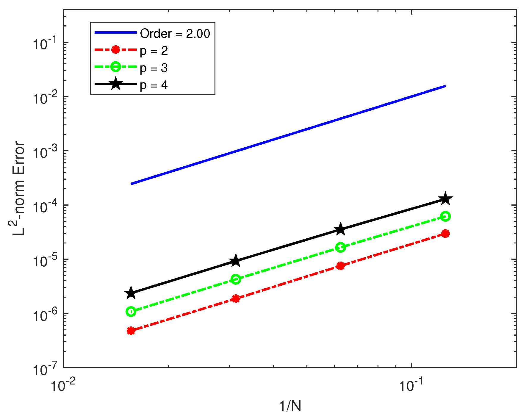
shows the errors and convergence orders in the spatial direction for different $\mu$ and p when fixing $N=512$, $\alpha =0.5$, and $\gamma =4$. It can be observed that regardless of whether $\mu$ changes or p changes, the spatial errors in the $L^2$-norm of the two schemes are similar and both can achieve fourth-order convergence in agreement with the theoretical prediction.

Table 3. Errors, convergence orders in space, and CPU times for the Alikhanov scheme and fast Alikhanov scheme by fixing $N=512$, $p=2$, $\mu =1$, and $\gamma =2$ for Example 1.

		$\mathit{\alpha }=0.3$		$\mathit{\alpha }=0.5$		$\mathit{\alpha }=0.7$
Alikhanov	$\mathit{M}$	${\mathit{E}}^{\mathbf{SOE}}(\mathit{M},\mathit{N})$	${\mathit{Rate}}_{\mathit{h}}^{\mathit{SOE}}$	${\mathit{E}}^{\mathit{SOE}}(\mathit{M},\mathit{N})$	${\mathit{Rate}}_{\mathit{h}}^{\mathit{SOE}}$	${\mathit{E}}^{\mathit{SOE}}(\mathit{M},\mathit{N})$	${\mathit{Rate}}_{\mathit{h}}^{\mathit{SOE}}$
	4	$4.6004\times {10}^{-3}$	-	$4.6355\times {10}^{-3}$	-	$4.5792\times {10}^{-3}$	-
	8	$2.8278\times {10}^{-4}$	4.0240	$2.8495\times {10}^{-4}$	4.0239	$2.8149\times {10}^{-4}$	4.0240
	16	$1.7600\times {10}^{-5}$	4.0061	$1.7735\times {10}^{-5}$	4.0060	$1.7555\times {10}^{-5}$	4.0031
	32	$1.0988\times {10}^{-6}$	4.0016	$1.1073\times {10}^{-6}$	4.0015	$1.1327\times {10}^{-6}$	3.9541
	CPU(s)	82.777		75.941		82.308
		$\alpha =0.3$		$\alpha =0.5$		$\alpha =0.7$
Fast Alikhanov	M	$E^{SOE}(M,N)$	$Rat{e}_h^{SOE}$	$E^{SOE}(M,N)$	$Rat{e}_h^{SOE}$	$E^{SOE}(M,N)$	$Rat{e}_h^{SOE}$
	4	$4.6004\times {10}^{-3}$	-	$4.6355\times {10}^{-3}$	-	$4.5792\times {10}^{-3}$	-
	8	$2.8278\times {10}^{-4}$	4.0240	$2.8495\times {10}^{-4}$	4.0239	$2.8145\times {10}^{-4}$	4.0241
	16	$1.7600\times {10}^{-5}$	4.0060	$1.7735\times {10}^{-5}$	4.0060	$1.7517\times {10}^{-5}$	4.0061
	32	$1.0997\times {10}^{-6}$	4.0005	$1.1073\times {10}^{-6}$	4.0015	$1.0939\times {10}^{-6}$	4.0011
	CPU(s)	3.9295		3.8685		3.9980

considers the cases where $N=512$, $p=2$, $\mu =1$, and $\gamma =2$ are fixed, with $\alpha$ changing, which indicates that the fast Alikhanov and Alikhanov schemes can achieve similar spatial errors and fourth-order convergence. The CPU times of the two algorithms are given; it is obvious that the fast Alikhanov scheme is much faster than the Alikhanov scheme. In order to further confirm whether the temporal and spatial convergence orders of the fast Alikhanov scheme remain stable as p increases, the temporal convergence and spatial convergence orders are shown in Figure 1 and Figure 2.

Table 4. Numerical solutions when $M=256$, $p=2$, $\mu =1$, and $\gamma =2/\alpha$ for Example 1.

	$\mathit{\alpha }=0.3$	$\mathit{\alpha }=0.5$	$\mathit{\alpha }=0.7$
$\mathit{N}$	$\mathit{U}$*	$\mathit{U}$*	$\mathit{U}$*
4	$1.4949$	$1.5049$	$1.4853$
8	$1.4950$	$1.5050$	$1.4853$
16	$1.4950$	$1.5050$	$1.4853$
32	$1.4950$	$1.5050$	$1.4853$
64	$1.4950$	$1.5050$	$1.4853$
128	$1.4950$	$1.5050$	$1.4853$

shows that with the gradual increase in N, the value of $U^{*}$ tends to stabilize and shows no increasing trend. These results confirm the numerical stability of the proposed scheme in the time direction.

Example 2. 

In order to verify the wide range of applications of the numerical scheme, the case where the exact solution is unknown is tested in this numerical example. We consider problems (1)–(3) in $\mathrm{\Omega }=(0,\pi )$ to verify the effectiveness and high accuracy of the numerical scheme. Let $T=1$, the initial condition is $u_0\left(x\right)=sin\left(x\right)$, and the source term is $f(x,t)=0$.

In

Table 5. Errors, convergence orders in space, and CPU times for the Alikhanov scheme and fast Alikhanov scheme by fixing $p=2$, $\mu =1$, $\gamma =2$, and $N=2048$ for Example 2.

		$\mathit{\alpha }=0.3$		$\mathit{\alpha }=0.5$		$\mathit{\alpha }=0.7$
Alikhanov	$\mathit{M}$	${\mathit{E}}^{\mathit{SOE}}(\mathit{M},\mathit{N})$	${\mathit{Rate}}_{\mathit{h}}^{\mathit{SOE}}$	${\mathit{E}}^{\mathit{SOE}}(\mathit{M},\mathit{N})$	${\mathit{Rate}}_{\mathit{h}}^{\mathit{SOE}}$	${\mathit{E}}^{\mathit{SOE}}(\mathit{M},\mathit{N})$	${\mathit{Rate}}_{\mathit{h}}^{\mathit{SOE}}$
	4	$4.3605\times {10}^{-4}$	-	$4.3568\times {10}^{-4}$	-	$4.5247\times {10}^{-4}$	-
	8	$2.6588\times {10}^{-5}$	4.0356	$2.6570\times {10}^{-5}$	4.0354	$2.7511\times {10}^{-5}$	4.0398
	16	$1.6529\times {10}^{-6}$	4.0077	$1.6517\times {10}^{-6}$	4.0078	$1.7094\times {10}^{-6}$	4.0084
	32	$1.0316\times {10}^{-7}$	4.0020	$1.0308\times {10}^{-7}$	4.0021	$1.0667\times {10}^{-7}$	4.0022
	CPU(s)	1253.8		1197.3		1279.9
		$\alpha =0.3$		$\alpha =0.5$		$\alpha =0.7$
Fast Alikhanov	M	$E^{SOE}(M,N)$	$Rat{e}_h^{SOE}$	$E^{SOE}(M,N)$	$Rat{e}_h^{SOE}$	$E^{SOE}(M,N)$	$Rat{e}_h^{SOE}$
	4	$4.3605\times {10}^{-4}$	-	$4.3568\times {10}^{-4}$	-	$4.5247\times {10}^{-4}$	-
	8	$2.6588\times {10}^{-5}$	4.0356	$2.6570\times {10}^{-5}$	4.0354	$2.7511\times {10}^{-5}$	4.0398
	16	$1.6529\times {10}^{-6}$	4.0077	$1.6517\times {10}^{-6}$	4.0078	$1.7094\times {10}^{-6}$	4.0084
	32	$1.0316\times {10}^{-7}$	4.0020	$1.0308\times {10}^{-7}$	4.0021	$1.0667\times {10}^{-7}$	4.0022
	CPU(s)	44.704		45.165		45.322

, the errors in the $L^2$-norm, spatial convergence orders, and CPU times of the Alikhanov scheme and the fast Alikhanov numerical scheme are presented for fixed values of $p=2$, $\mu =1$, $\gamma =2$, and $N=2048$, with $\alpha \in \{0.3,0.5,0.7\}$. It is worth mentioning that both numerical schemes can achieve the same approximation effect, but the CPU time of the fast scheme is much shorter.

Table 6. The $E^{SOE}$-norm errors and temporal convergence orders with $M=512$, $\mu =1$, $\alpha =0.8$, and $\gamma =2/\alpha$.

	$\mathit{p}=1$		$\mathit{p}=2$		$\mathit{p}=3$		$\mathit{p}=4$		$\mathit{p}=5$
$\mathit{N}$	${\mathit{E}}^{\mathit{SOE}}(\mathit{M},\mathit{N})$	${\mathit{Rate}}_{\mathit{\tau }}^{\mathit{SOE}}$	${\mathit{E}}^{\mathit{SOE}}(\mathit{M},\mathit{N})$	${\mathit{Rate}}_{\mathit{\tau }}^{\mathit{SOE}}$	${\mathit{E}}^{\mathit{SOE}}(\mathit{M},\mathit{N})$	${\mathit{Rate}}_{\mathit{\tau }}^{\mathit{SOE}}$	${\mathit{E}}^{\mathit{SOE}}(\mathit{M},\mathit{N})$	${\mathit{Rate}}_{\mathit{\tau }}^{\mathit{SOE}}$	${\mathit{E}}^{\mathit{SOE}}(\mathit{M},\mathit{N})$	${\mathit{Rate}}_{\mathit{\tau }}^{\mathit{SOE}}$
10	$1.3260\times {10}^{-3}$	-	$1.3265\times {10}^{-3}$	-	$1.3266\times {10}^{-3}$	-	$1.3266\times {10}^{-3}$	-	$1.3266\times {10}^{-3}$	-
20	$3.4271\times {10}^{-4}$	1.9520	$3.4279\times {10}^{-4}$	1.9522	$3.4281\times {10}^{-4}$	1.9522	$3.4281\times {10}^{-4}$	1.9522	$3.4281\times {10}^{-4}$	1.9523
40	$9.0337\times {10}^{-5}$	1.9236	$9.0353\times {10}^{-5}$	1.9237	$9.0356\times {10}^{-5}$	1.9237	$9.0354\times {10}^{-5}$	1.9238	$9.0351\times {10}^{-5}$	1.9238
80	$2.3914\times {10}^{-5}$	1.9174	$2.3917\times {10}^{-5}$	1.9176	$2.3917\times {10}^{-5}$	1.9176	$2.3914\times {10}^{-5}$	1.9177	$2.3914\times {10}^{-5}$	1.9177
160	$6.3120\times {10}^{-6}$	1.9217	$6.3132\times {10}^{-6}$	1.9216	$6.3131\times {10}^{-6}$	1.9216	$6.3145\times {10}^{-6}$	1.9211	$6.3158\times {10}^{-6}$	1.9208

demonstrates that for fixed values of $M=512$, $\mu =1$, $\alpha =0.8$, and $\gamma =2/\alpha$, the $L^2$-norm error decreases as the number of temporal subintervals increases. It is expected that the convergence order of the fast approximate scheme is $\mathcal{O}\left({\tau }^2\right)$. Meanwhile, the error and convergence order remain as expected for changing values of p, suggesting that the approximation scheme is stable for different p.

Table 7. The $E^{SOE}$-norm errors, temporal convergence orders, and CPU time (seconds) with $M=512$, $p=2$, and $\gamma =2/\alpha$.

	$\mathit{\mu }=0.05$			$\mathit{\mu }=0.1$
$\mathit{N}$	${\mathit{E}}^{\mathit{SOE}}(\mathit{M},\mathit{N})$	${\mathit{Rate}}_{\mathit{\tau }}^{\mathit{SOE}}$	CPU(s)	$\mathit{N}$	${\mathit{E}}^{\mathit{SOE}}(\mathit{M},\mathit{N})$	${\mathit{Rate}}_{\mathit{\tau }}^{\mathit{SOE}}$	CPU(s)
4	$2.8796\times {10}^{-3}$	-	0.4605	4	$3.2656\times {10}^{-3}$	-	0.4406
8	$6.8144\times {10}^{-4}$	2.0792	0.7595	8	$7.7751\times {10}^{-4}$	2.0704	0.8029
16	$1.7604\times {10}^{-4}$	1.9527	1.5174	16	$2.0089\times {10}^{-4}$	1.9525	1.5480
32	$4.8379\times {10}^{-5}$	1.8634	2.5469	32	$5.4828\times {10}^{-5}$	1.8734	2.7098
64	$1.3632\times {10}^{-5}$	1.8273	5.0930	64	$1.5262\times {10}^{-5}$	1.8450	5.3880
	$\mu =1$			$\mu =2$
N	$E^{SOE}(M,N)$	$Rat{e}_{\tau }^{SOE}$	CPU(s)	N	$E^{SOE}(M,N)$	$Rat{e}_{\tau }^{SOE}$	CPU(s)
4	$8.7476\times {10}^{-3}$	-	0.4646	4	$9.7976\times {10}^{-3}$	-	0.5341
8	$2.0697\times {10}^{-3}$	2.0794	0.7903	8	$2.3022\times {10}^{-3}$	2.0894	0.7326
16	$5.2813\times {10}^{-4}$	1.9705	1.4359	16	$5.8600\times {10}^{-4}$	1.9741	1.3253
32	$1.3868\times {10}^{-4}$	1.9291	2.6138	32	$1.5258\times {10}^{-4}$	1.9413	2.5373
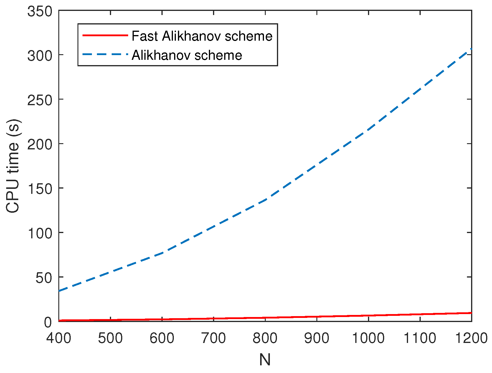
64	$3.6684\times {10}^{-5}$	1.9185	5.0402	64	$3.9897\times {10}^{-5}$	1.9353	4.7893

shows the errors, temporal convergence orders, and CPU times for different $\mu$, where we take $M=512$, $p=2$, and $\gamma =2/\alpha$. In each row of the table, the errors and convergence orders change very little as $\mu$ varies, so the method is stable for the coefficient $\mu$, as predicted by our theoretical analysis. In addition, in order to demonstrate more intuitively the speedup effect of the SOE approximation, taking $\alpha =0.5,p=2,\mu =1,\gamma =2$, and $M=4$, we plot the computation time curves of the two schemes for the N increase, as shown in Figure 3. It is clear that the fast Alikhanov scheme saves a lot of computational costs compared to the Alikhanov scheme.

Example 3. 

In this example, we consider problem (1) over domains $\mathrm{\Omega }=(0,1)$ and $T=1$. The analytic solution is $u(x,t)=\left({\displaystyle \frac{t^{\alpha }}{\mathrm{\Gamma }(1+\alpha )}}\right)sin\left(\pi x\right)cos\left(\pi x\right)$, such that the source term $f(x,t)$ is as follows:

$$\begin{array}{cc}\hfill f(x,t)& =sin\left(\pi x\right)cos\left(\pi x\right)+2{\pi }^2\mu {\displaystyle \frac{t^{\alpha }}{\mathrm{\Gamma }(1+\alpha )}}sin\left(2\pi x\right)+8{\pi }^4{\displaystyle \frac{t^{\alpha }}{\mathrm{\Gamma }(1+\alpha )}}sin\left(2\pi x\right)\hfill \\ \hfill & +\pi {\left({\displaystyle \frac{t^{\alpha }}{\mathrm{\Gamma }(1+\alpha )}}\right)}^{p+1}{(sin\left(\pi x\right))}^p{(cos\left(\pi x\right))}^{p}cos\left(2\pi x\right).\hfill \end{array}$$

Table 8. Errors, temporal convergence orders, and CPU times by fixing $p=2$, $\mu =1$, $\gamma =4$, and $M=256$ for Example 3.

	$\mathit{\alpha }=0.3$			$\mathit{\alpha }=0.5$			$\mathit{\alpha }=0.7$
$\mathit{N}$	${\mathit{E}}^{\mathit{SOE}}(\mathit{M},\mathit{N})$	${\mathit{Rate}}_{\mathit{\tau }}^{\mathit{SOE}}$	CPU	${\mathit{E}}^{\mathit{SOE}}(\mathit{M},\mathit{N})$	${\mathit{Rate}}_{\mathit{\tau }}^{\mathit{SOE}}$	CPU	${\mathit{E}}^{\mathit{SOE}}(\mathit{M},\mathit{N})$	${\mathit{Rate}}_{\mathit{\tau }}^{\mathit{SOE}}$	CPU
16	$9.5519\times {10}^{-7}$	-	0.2818	$3.9181\times {10}^{-6}$	-	0.2457	$8.5622\times {10}^{-6}$	-	0.2060
32	$2.4356\times {10}^{-7}$	1.9715	0.4170	$1.0148\times {10}^{-6}$	1.9490	0.3583	$2.2256\times {10}^{-6}$	1.9438	0.4410
64	$5.8573\times {10}^{-8}$	2.0560	0.7595	$2.5816\times {10}^{-7}$	1.9748	0.7026	$5.6804\times {10}^{-7}$	1.9701	0.7078
128	$1.6584\times {10}^{-8}$	1.8205	1.8818	$6.6561\times {10}^{-8}$	1.9555	1.4596	$1.4255\times {10}^{-7}$	1.9946	1.5336

and

Table 9. Errors, convergence orders in space, and CPU times by fixing $p=2$, $\mu =1$, $\gamma =4$, and $N=1000$ for Example 3.

	$\mathit{\alpha }=0.3$			$\mathit{\alpha }=0.5$			$\mathit{\alpha }=0.7$
$\mathit{M}$	${\mathit{E}}^{\mathit{SOE}}(\mathit{M},\mathit{N})$	${\mathit{Rate}}_{\mathit{h}}^{\mathit{SOE}}$	CPU	${\mathit{E}}^{\mathit{SOE}}(\mathit{M},\mathit{N})$	${\mathit{Rate}}_{\mathit{h}}^{\mathit{SOE}}$	CPU	${\mathit{E}}^{\mathit{SOE}}(\mathit{M},\mathit{N})$	${\mathit{Rate}}_{\mathit{h}}^{\mathit{SOE}}$	CPU
16	$7.7546\times {10}^{-5}$	-	13.587	$7.8530\times {10}^{-5}$	-	13.533	$7.6592\times {10}^{-5}$	-	13.994
32	$4.8243\times {10}^{-6}$	4.0067	15.856	$4.8854\times {10}^{-6}$	4.0067	15.493	$4.7648\times {10}^{-6}$	4.0067	15.609
64	$3.0131\times {10}^{-7}$	4.0010	19.515	$3.0497\times {10}^{-7}$	4.0017	19.445	$2.9744\times {10}^{-7}$	4.0017	19.734
128	$1.9031\times {10}^{-8}$	3.9848	28.411	$1.9111\times {10}^{-8}$	3.9962	28.621	$1.8807\times {10}^{-8}$	3.9833	28.510

display the temporal and spatial errors, spatial–temporal convergence orders, and CPU times for various $\alpha$ values. Furthermore, the results show that the proposed scheme can reach the second order of convergence in time and the fourth order of convergence in space. Next, we test the stability by fixing $M=256$, $\mu =1$, $p=2$, and $\gamma =2/\alpha$ and selecting different T values, which means the time-step sizes are different. The numerical results are listed in

Table 10. The $E_2$-norm errors and temporal convergence orders with $M=256$, $\mu =1$, $p=2$, and $\gamma =2/\alpha$.

	$\mathit{T}=0.5$		$\mathit{T}=1$		$\mathit{T}=4$		$\mathit{T}=10$
$\mathit{N}$	${\mathit{E}}^{\mathit{SOE}}(\mathit{M},\mathit{N})$	${\mathit{Rate}}_{\mathit{\tau }}^{\mathit{SOE}}$	${\mathit{E}}^{\mathit{SOE}}(\mathit{M},\mathit{N})$	${\mathit{Rate}}_{\mathit{\tau }}^{\mathit{SOE}}$	${\mathit{E}}^{\mathit{SOE}}(\mathit{M},\mathit{N})$	${\mathit{Rate}}_{\mathit{\tau }}^{\mathit{SOE}}$	${\mathit{E}}^{\mathit{SOE}}(\mathit{M},\mathit{N})$	${\mathit{Rate}}_{\mathit{\tau }}^{\mathit{SOE}}$
16	$1.3810\times {10}^{-6}$	-	$3.9181\times {10}^{-6}$	-	$3.1501\times {10}^{-5}$	-	$1.2475\times {10}^{-4}$	-
32	$3.5931\times {10}^{-7}$	1.9424	$1.0148\times {10}^{-6}$	1.9490	$8.1468\times {10}^{-6}$	1.9511	$3.2269\times {10}^{-5}$	1.9507
64	$9.0207\times {10}^{-8}$	1.9939	$2.5816\times {10}^{-7}$	1.9748	$2.0664\times {10}^{-6}$	1.9791	$8.2114\times {10}^{-6}$	1.9745
128	$2.3438\times {10}^{-8}$	1.9444	$6.6561\times {10}^{-8}$	1.9555	$5.2247\times {10}^{-7}$	1.9837	$2.0765\times {10}^{-6}$	1.9835
256	$6.0047\times {10}^{-9}$	1.9647	$1.5317\times {10}^{-8}$	2.1196	$1.3334\times {10}^{-7}$	1.9703	$5.2527\times {10}^{-7}$	1.9830

, which shows that the fast Alikhanov scheme is stable and has a relaxed stability restriction. In

Table 11. The $E_2$-norm errors and temporal convergence orders with $M=256$, $\mu =1$, $p=2$, $\alpha =0.5$, and $\gamma =2/\alpha$.

	$\mathit{\alpha }=0.95$		$\mathit{\alpha }=0.99$		$\mathit{\alpha }=0.999$		$\mathit{\alpha }=0.9999$
$\mathit{N}$	${\mathit{E}}^{\mathit{SOE}}(\mathit{M},\mathit{N})$	${\mathit{Rate}}_{\mathit{\tau }}^{\mathit{SOE}}$	${\mathit{E}}^{\mathit{SOE}}(\mathit{M},\mathit{N})$	${\mathit{Rate}}_{\mathit{\tau }}^{\mathit{SOE}}$	${\mathit{E}}^{\mathit{SOE}}(\mathit{M},\mathit{N})$	${\mathit{Rate}}_{\mathit{\tau }}^{\mathit{SOE}}$	${\mathit{E}}^{\mathit{SOE}}(\mathit{M},\mathit{N})$	${\mathit{Rate}}_{\mathit{\tau }}^{\mathit{SOE}}$
16	$4.0608\times {10}^{-6}$	-	$3.8864\times {10}^{-6}$	-	$3.8417\times {10}^{-6}$	-	$3.8366\times {10}^{-6}$	-
32	$1.0171\times {10}^{-6}$	1.9973	$9.7447\times {10}^{-6}$	1.9957	$9.6418\times {10}^{-7}$	1.9944	$9.6071\times {10}^{-7}$	1.9977
64	$2.5443\times {10}^{-7}$	1.9992	$2.4199\times {10}^{-7}$	2.0097	$2.4196\times {10}^{-7}$	1.9946	$2.3883\times {10}^{-7}$	2.0081
128	$6.5139\times {10}^{-8}$	1.9657	$6.0890\times {10}^{-8}$	1.9907	$6.0593\times {10}^{-8}$	1.9975	$5.8879\times {10}^{-8}$	2.0201
256	$1.6078\times {10}^{-8}$	2.0184	$1.5477\times {10}^{-8}$	1.9761	$1.7048\times {10}^{-8}$	1.8295	$1.4500\times {10}^{-8}$	2.0217

, we tested the errors for $\alpha =0.95,\alpha =0.99,\alpha =0.999,\mathrm{and}\alpha =0.9999$ by making $M=256$, $\mu =1$, $p=2$, and $\gamma =2/\alpha$, which also shows that the numerical scheme is stable when ${\displaystyle \alpha \to 1^{-}}$.

5. Conclusions

In this work, we propose a fast high-order compact scheme for solving the fractional KS equation with the generalized Burgers’ type nonlinearity. To deal with the weak singularity at the initial time, the Alikhanov scheme is implemented to approximate the Caputo fractional derivative in the time direction. With the aid of the SOE technique, the computational efficiency is improved and the storage requirement is reduced. In the space direction, the developed compact difference formulas have been successfully applied for approximating the spatial derivatives. As a result, a fully discrete scheme is constructed. Meanwhile, the stability and convergence with ${\tau }^2+h^4$ of the proposed scheme are proved. Finally, the results of the numerical experiments demonstrate that the convergence orders for temporal and spatial convergence achieve second-order and fourth-order accuracies, respectively. This is highly consistent with the theoretical predictions and effectively verifies the theoretical analysis.