Certain Analytic Solutions for Time-Fractional Models Arising in Plasma Physics via a New Approach Using the Natural Transform and the Residual Power Series Methods

Abstract

This paper studies three time-fractional models that arise in plasma physics: the modified Korteweg–deVries–Zakharov–Kuznetsov equation, the stochastic potential Korteweg–deVries equation, and the forced Korteweg–deVries equation. These equations are significant in plasma physics for modeling nonlinear ion acoustic waves and thus helping us to understand wave dynamics in plasmas. We introduce a new approach that relies on a new fractional expansion in the natural transform space and residual power series method to construct analytical solutions to the governing models. We investigate the theoretical analysis of the proposed method for these equations to expose this approach’s applicability, efficiency, and effectiveness in constructing analytical solutions to the governing equations. Moreover, we present a comparative discussion between the solutions derived during the work and those given in the literature to confirm that the proposed approach generates analytical solutions that rapidly converge to exact solutions, which proves the effectiveness of the proposed method.

1. Introduction

Nonlinear wave phenomena are of fundamental importance in the context of physics in general and plasma dynamics in particular [1]. A comprehensive understanding of ion acoustic waves and their behavior is essential for many applications in the context of plasma physics, such as energy transfer, plasma containment, and wave–particle interactions [2,3]. In light of this, many mathematical models have been presented to describe such phenomena, including the Korteweg–de Vries (KdV) equation [4], the nonlinear Schrödinger equation [5], Burgers’ equation [6], the Zakharov system [7], the sine-Gordon equation [8], the Benjamin–Bona–Mahony equation [9], the Kadomtsev–Petviashvili equation [10], and others. Since the emergence of the concept of fractional differential and integral calculus and the work carried out by researchers in studying its impact on mathematical systems in various fields of science, researchers have turned their attention to researching the importance of fractional differential and integral calculus in plasma physics [11,12]. It has been shown that fractional calculations have great importance for the effects of memory and generic properties of systems, which play a prominent role in providing an accurate description of complex plasma dynamics [13,14]. Considering the long-term interactions in plasma systems, the fractional derivative provides a more general approach than classical derivatives, which in turn helps in modeling the wave propagation, diffusion processes, and anomalous transport phenomena that may not be available in standard models to capture the complex behavior of plasma [15]. This enables scientists to gain a deeper understanding of plasma behavior in physical environments and laboratories by developing fractional mathematical models for ion acoustic waves, plasma turbulence, and other nonlinear phenomena [16]. The main interest of this work is to study three important equations in the context of plasma physics: the fractional modified Korteweg–deVries–Zakharov–Kuznetsov (mKdV-ZK) equation, the fractional stochastic potential Korteweg–deVries (spKdV) equation, and the fractional forced Korteweg–deVries (FKdV) equation. We consider the following time-fractional KdV-ZK equation [17]:

$${\mathcal{D}}_t^{\alpha }\psi +{\mu }^2\psi {\displaystyle \frac{\partial \psi }{\partial x}}+{\displaystyle \frac{{\partial }^3\psi }{\partial x^3}}+{\displaystyle \frac{{\partial }^3\psi }{\partial x\partial y^2}}+{\displaystyle \frac{{\partial }^3\psi }{\partial x\partial z^2}}=0, t\ge 0, x,y,z\in \mathbb{R},$$

(1.1)

subject to the initial condition:

$$\psi (x,y,z,0)=f\left(x,y,z\right),x,y,z\in \mathbb{R},$$

(1.2)

where ${\mathcal{D}}_t^{\alpha }\psi$ represents the Caputo derivative of the electric field potential $\psi \left(x,y,z,t\right)$ with respect to the time $t$ of the fractional derivative order $\alpha \in (0,1]$. The variables $x,y$ and $z$ are the scaled space coordinates, while $\mu$ is the dispersion coefficient that stands for positive correlation with negative correlation, Boltzmann distribution, and fluid species. The Korteweg–DeVries–Zakharov–Kuznetsov equation was introduced by the authors [18] with the aim of using the reductive perturbation approach for mixing both warm adiabatic fluids and cold stationary isothermal solid background species in a magnetized plasma where they discussed acoustic electron, acoustic ion, and acoustic dust waves. In Ref. [19], the mKdV-ZK equation is presented using the reductive perturbation approach to control the diagonal diffusion in nonlinear electrostatic modes. In Ref. [20], multiple-soliton solutions for the mKdV-ZK equation were obtained. Solitary solutions were explored using the modified extended direct algebraic method for the mKdV-ZK equation in Ref. [21]. Younas et al. constructed traveling wave solutions by utilizing two different approaches to the mKdV-ZK equation [22]. The second equation considered in this work is the time-fractional spKdV equation [23]:

$${\mathcal{D}}_t^{\alpha }\psi +\omega {\displaystyle \frac{\partial \psi }{\partial x}}+\beta {\left({\displaystyle \frac{\partial \psi }{\partial x}}\right)}^2+\gamma {\displaystyle \frac{{\partial }^3\psi }{\partial x^3}}=0, t\ge 0, x\in \mathbb{R},$$

(1.3)

subject to the initial condition:

$$\psi \left(x,0\right)=g\left(x\right),x\in \mathbb{R},$$

(1.4)

where $\omega$ is the stochastic parameter, $\beta$ is the nonlinearity coefficient, and $\gamma$ refers to the dispersion coefficient. Equation (1.3) is a nonlinear model that appears in applications of multicomponent plasmas and electrical circuits and is used to predict the weak dispersive effects on the propagation of nonlinear optical waves and photons. The spKdV equation is presented in Ref. [23], where the authors obtained lumps, breathers, and multi-soliton solutions using the simplified Hirota method and the Cole–Hopf transformation. In Ref. [24], the authors suggested the fractional spKdV equation and they constructed closed-form solutions for the proposed model. In Ref. [25], the spKdV equation was investigated and the Lie symmetry approach was utilized to carry out the symmetry generators to obtain traveling wave solutions and conservation laws for the proposed model. The final equation that will be investigated in our paper is the following fractional FKdV equation [26]:

$${\displaystyle \frac{1}{c}}{\mathcal{D}}_t^{\alpha }\psi +\left(\left({\mathcal{F}}_r-1\right)-{\displaystyle \frac{3}{2\chi }}\psi \right){\displaystyle \frac{\partial \psi }{\partial x}}-{\displaystyle \frac{{\chi }^2}{6}}{\displaystyle \frac{{\partial }^3\psi }{\partial x^3}}={\displaystyle \frac{1}{2}}{\displaystyle \frac{d\varphi \left(x\right)}{dx}}, t\ge 0, x\in \mathbb{R},$$

(1.5)

subject to the initial condition:

$$\psi \left(x,0\right)=h\left(x\right),x\in \mathbb{R}.$$

(1.6)

The term $\left(\left({\mathcal{F}}_r-1\right)-{\displaystyle \frac{3}{2\chi }}\psi \right){\displaystyle \frac{\partial \psi }{\partial x}}$ describes nonlinear interactions in a wave that are measured using the parameter $\chi$ which arises from the amplitude of the plasma wave where higher amplitudes affect the wave velocity. The parameter ${\mathcal{F}}_r$ represents some force or property of the plasma. The term ${\displaystyle \frac{1}{2}}{\displaystyle \frac{d\varphi \left(x\right)}{dx}}$ represents an external influence on the plasma wave such as an electric or magnetic field or any other disturbance. The importance of Equation (1.5) lies in allowing the integration of external forces, memory effects, nonlinearity, and dispersion to model the propagation of nonlinear ion-acoustic waves, as these components are necessary to accurately describe the wave behavior in plasma environments. This model is of great value in many contexts such as astrophysical plasmas affected by large-scale forces, fusion plasmas affected by electric and magnetic fields, and the study of stability and turbulence in plasma systems. In Ref. [26], the authors investigated the fractional FKdV equation to construct traveling wave solutions using the fractional natural decomposition method. The distributed-order time-fractional FKdV equation is presented in Ref. [27], where the authors used the shifted Legendre operational matrix to infer approximate solutions for the proposed model. In Ref. [28], the authors studied the FKdV equation and obtained approximate solutions for the model using the q-homotopy analysis transform technique. The fractional FKdV equation was discussed with the help of the Yang homotopy perturbation method and the Yang transform decomposition method to construct approximate solutions for the model in Ref. [29].

With the wide development in scientific research regarding mathematical systems that describe and model physical phenomena and the emergence and discovery of complex systems in various fields of science, the need to develop methods to derive accurate and approximate solutions for these presented systems arose. Researchers worked to develop such techniques, including the reproducing kernel Hilbert space method [30], the multistep reduced differential transformation method [31], the Atangana–Baleanu fractional framework for the reproducing kernel technique [32], the multistep generalized differential transform method [33], the homotopy analysis method [34], the shifted Jacobi polynomials method [35], the Chebyshev polynomials method [36], auxiliary equation method [37], the B-spline schemes method [38], the fractional variational iteration method [39,40,41], the Kudryashov method [42], and others. Abu Arqub et al. [43] presented a new analytical method, the residual power series (RPS) method, for obtaining solitary wave solutions of time-fractional dispersive partial differential equations based on the generalized Taylor series formula and residual error function. Researchers have employed this method to derive analytical solutions for a wide range of fractional equations as it is an effective method [44,45]. In Ref. [46], El-Ajou proposed a new technique that combines the Laplace transform and RPS method, called the Laplace residual power series (LRPS) method, where the proposed method was utilized to explore exact solitary solutions to the nonlinear time-fractional dispersive partial differential equations (PDEs). The main goal of this work is to suggest a new attractive approach, the natural residual power series (NRPS) method, that depends on the natural transformation and RPS method. Moreover, we seek to utilize the NRPS method to infer analytical solutions for the governing Equations (1.1)–(1.6). The NRPS method is based on using natural transformation to transform the time-fractional differential equation into the natural space, then using a suitable expansion to deal with the newly obtained equation together with the RPS method, which in turn helps in deducing the expansion coefficients based on the concept of limit, which reduces the calculations required to reach accurate approximate solutions to the governing equation.

We organized the paper with the introduction as the first section. Section 2 presents some preliminaries about the Caputo fractional derivative. Section 3 is devoted to introducing the definition of natural transformation and investigating its essential properties, then presenting the natural fractional expansion. In Section 4, we introduce the steps of the proposed method. Applications of the NRPS method to construct approximate solutions for the governing models are introduced in Section 5. Some conclusions are presented in Section 6.

2. Preliminaries

Since the advent of fractional calculus, many fractional operators have appeared, such as the Riemann–Liouville operator [47], the Caputo operator [48], Atangana–Baleanu operator [49], and others. Here, we present the definition of the Caputo fractional derivative and some of its essential properties that are useful in our work.

Definition 1

([49]). The Caputo derivative of fractional order $\alpha >0$ of an integrable function $\psi \left(t\right)$ is given by:

$${\mathcal{D}}_t^{\alpha }\psi \left(t,x\right)={\displaystyle \frac{1}{\mathsf{\Gamma }\left(k-\alpha \right)}}\underset{0}{\overset{t}{\int }}{\displaystyle \frac{\frac{{\partial }^k\psi (\tau ,x)}{\partial {\tau }^k }}{{\left(t-\tau \right)}^{\alpha -k+1}}}d\tau ,$$

(2.1)

where $t\ge 0, k=\left[\alpha \right]+1$. The Riemann–Liouville fractional integral of order $\alpha , Re\left(\alpha \right)>0$ is given by:

$${\mathcal{J}}_t^{\alpha }\psi \left(t\right)={\displaystyle \frac{1}{\mathsf{\Gamma }\left(\alpha \right)}}\underset{0}{\overset{t}{\int }}{\left(t-\tau \right)}^{\alpha -1}\psi \left(\tau ,x\right)d\tau .$$

(2.2)

Lemma 1

([49]). For $\alpha >0, \eta >-1, p\in \mathbb{R}$ and $t\ge 0$, the Caputo fractional derivative has the property:

$$\begin{array}{}\hfill \text{(2.3)}\hfill & \hfill \text{(a)}\hfill & {\mathcal{D}}_t^{\alpha }p=0.\hfill \hfill \text{(2.4)}\hfill & \hfill \text{(b)}\hfill & {\mathcal{D}}_t^{\alpha }{t}^{\eta }={\displaystyle \frac{\mathsf{\Gamma }\left(\eta +1\right)}{\mathsf{\Gamma }\left(\eta +1-\alpha \right)}}{t}^{\eta -\alpha }.\hfill \hfill \text{(2.5)}\hfill & \hfill \text{(c)}\hfill & {\mathcal{D}}_t^{\alpha }{\mathcal{J}}_t^{\alpha }\psi \left(t,x\right)=\psi \left(t,x\right).\hfill \hfill \text{(2.6)}\hfill & \hfill \text{(d)}\hfill & {\mathcal{J}}_t^{\alpha }{\mathcal{D}}_t^{\alpha }\psi \left(t,x\right)=\psi \left(t,x\right)-{\displaystyle \sum _{i=0}^{k-1}}{\displaystyle \frac{{\partial }^i\psi \left(0^{+},x\right)}{\partial t^i}} {\displaystyle \frac{t^i}{i!}}.\hfill \end{array}$$

3. Natural Transformation and Fractional Expansion

The natural transformation combines the features of the Laplace and the Sumudu transforms into a powerful tool for dealing with a variety of differential and integral equations. Natural transformation provides a simple and flexible approach to transforming functions from the time domain to the complex domain, making it powerful for dealing with problems involving fractional time models. Furthermore, the natural transform can handle a wide range of functions with singularities and simplifies the process of finding analytical solutions to complex problems. Therefore, it is considered a valuable tool widely used in applied mathematics, engineering, and physics [50,51,52,53,54]. The general integral transform of the function $\psi \left(t,x\right), t,x\in \mathbb{R}$ is defined as:

$$\mathcal{T}\left\{\psi \left(t,x\right)\right\}=\underset{-\infty }{\overset{\infty }{\int }}\mathcal{K}\left(s,t\right)\psi \left(t,x\right)dt,$$

(3.1)

where $\mathcal{K}\left(s,t\right)$ is the kernel of the transform and $s$ represents the real (complex) number that is independent of $t$. The Laplace transform, Mellin transform, and Hankel transform can be obtained by letting the kernel of the transform in (3.1) be: $e^{-st}, t^{s-1}\left(st\right)$, and $t{J}_n\left(st\right)$, respectively. To define the natural transformation, we define the following set:

$$\mathcal{C}=\left\{\psi \left(t,x\right):\exists B, {\sigma }_1,{\sigma }_2, \left|\psi \left(t,x\right)\right|<B{e}^{\left({\displaystyle \frac{\left|t\right|}{{\sigma }_i}}\right)},t\in {\left(-1\right)}^i\times \left[0,\infty \right), x\in A\subseteq \mathbb{R},i\in {\mathbb{Z}}^{+}\right\}$$

(3.2)

Definition 2

([51]). Let $\psi \left(t,x\right)\in \mathcal{C}$. The natural transformation of the function $\psi \left(t,x\right)$ is defined as:

$$\mathsf{\Psi }\left(s,w,x\right)=\mathcal{N}\left\{\psi \left(t,x\right)\right\}=\underset{0}{\overset{\infty }{\int }}{e}^{-st}\psi \left(wt,x\right)dt, s,w\in (0,\infty ),$$

(3.3)

where $\mathcal{N}\left\{\psi \left(t,x\right)\right\}$ is the natural transformation of $\psi \left(t,x\right)$ and the variables $s$ and $w$ are the natural transform variables. The inverse natural transformation of the function $\Psi \left(s,w,x\right)$ is defined as follows:

$$\psi \left(t,x\right)={\mathcal{N}}^{-1}\left\{\mathsf{\Psi }\left(s,w,x\right)\right\}={\displaystyle \frac{1}{2\pi i}}\underset{u-i\infty }{\overset{u+i\infty }{\int }}{e}^{-{\displaystyle \frac{st}{w}}}\mathsf{\Psi }\left(s,w,x\right)ds, t\in \left[0,\infty \right),$$

(3.4)

where the integral is applied for a complex number $s=a+ib$ along $s=u$.

The following theorem shows the existence of natural transformations.

Theorem 1

([51]). Let $\psi \left(t,x\right)\in \mathcal{C}$ be piecewise continuous on $\left[0,\infty \right)\times A$ and of an exponential order ${\displaystyle \frac{\theta }{w}}$ as $t\to \infty$. Then, the natural transformation of $\psi \left(t,x\right)$ exists for all $s\in \left(\theta ,\infty \right),w\in \left(0,\infty \right)$.

Remark 1.

The Laplace and Sumudu transforms can be obtained by letting $w=1$ and $s=1$, respectively, in the natural transform (3.3).

Remark 2.

Let $\mathsf{\Psi }\left(s,w,x\right)=\mathcal{N}\left\{\psi \left(t,x\right)\right\}$ be the natural transform of the function and let

$${\mathsf{\Psi }}_L\left(s,x\right)=\mathcal{L}\left\{\psi \left(t,x\right)\right\}=\underset{0}{\overset{\infty }{\int }}{e}^{-st}\psi \left(t,x\right)dt,$$

$${\mathsf{\Psi }}_S\left(w,x\right)=\mathcal{S}\left\{\psi \left(t,x\right)\right\}=\underset{0}{\overset{\infty }{\int }}{e}^{-t}\psi \left(wt,x\right)dt,$$

be the Laplace and Sumudu transforms of the function $\psi \left(t,x\right)$, respectively. Then, the duality relationship between the Natural-Laplace and Natural-Sumudu transforms is given by:

$$\mathcal{N}\left\{\psi \left(t,x\right)\right\}=\mathsf{\Psi }\left(s,w,x\right)={\displaystyle \frac{1}{w}}{\mathsf{\Psi }}_L\left({\displaystyle \frac{s}{w}},x\right),$$

(3.5)

$$\mathcal{N}\left\{\psi \left(t,x\right)\right\}=\mathsf{\Psi }\left(s,w,x\right)={\displaystyle \frac{1}{s}}{\mathsf{\Psi }}_S\left({\displaystyle \frac{w}{s}},x\right).$$

(3.6)

Lemma 2

([52]). Let ${\psi }_1\left(t,x\right),{\psi }_2\left(t,x\right)\in \mathcal{C}$ be piecewise continuous on $\left[0,\infty \right)\times A$ and of an exponential order ${\displaystyle \frac{{\theta }_1}{w}}$ and ${\displaystyle \frac{{\theta }_2}{w}}$, respectively, with ${\theta }_1<{\theta }_2$. Then, the natural transform satisfies the following properties:

$$\begin{array}{}\hfill \text{(3.7)}\hfill & \hfill \text{(i)}\hfill & \mathcal{N}\left(1\right)={\displaystyle \frac{1}{s}}.\hfill \hfill \text{(3.8)}\hfill & \hfill \text{(ii)}\hfill & \mathcal{N}\left(t^{k\eta }\right)={\displaystyle \frac{\mathsf{\Gamma }\left(k\eta +1\right)w^{k\eta }}{s^{k\eta +1}}}, \eta >-1.\hfill \hfill \text{(3.9)}\hfill & \hfill \text{(iii)}\hfill & \mathcal{N}\left(p_1{\psi }_1\left(t,x\right)+p_2{\psi }_2\left(t,x\right)\right)=p_1{\mathsf{\Psi }}_1\left(s,w,x\right)+p_2{\mathsf{\Psi }}_2\left(s,w,x\right), p_1,p_2\in \mathbb{R}.\hfill \hfill \text{(3.10)}\hfill & \hfill \text{(iv)}\hfill & {\mathcal{N}}^{-1}\left(p_1{\mathsf{\Psi }}_1\left(s,w,x\right)+p_2{\mathsf{\Psi }}_2\left(s,w,x\right)\right)=p_1{\psi }_1\left(t,x\right)+p_2{\psi }_1\left(t,x\right), p_1,p_2\in \mathbb{R}.\hfill \end{array}$$

Lemma 3.

Let $\psi \left(t,x\right)\in \mathcal{C}$ be piecewise continuous on $\left[0,\infty \right)\times A$ and of exponential order ${\displaystyle \frac{\theta }{w}}$. Then, the natural transform satisfies the following properties:

$$\begin{array}{}\hfill \text{(3.11)}\hfill & \hfill \text{(i)}\hfill & \mathcal{N}\left\{{\displaystyle \frac{{\partial }^k}{\partial t^k}}\psi \left(t,x\right)\right\}={\displaystyle \frac{s^k}{w^k}}\mathsf{\Psi }\left(s,w,x\right)-{\displaystyle \sum _{i=0}^{k-1}}{\displaystyle \frac{s^{k-i-1}}{w^{k-i}}}{\displaystyle \frac{{\partial }^i}{\partial t^i}}\psi \left(0,x\right),k\in \mathbb{Z}.\hfill \hfill \text{(3.12)}\hfill & \hfill \text{(ii)}\hfill & \underset{s\to \infty }{\lim }s\mathsf{\Psi }\left(s,w,x\right)=\psi \left(0,x\right).\hfill \hfill \text{(3.13)}\hfill & \hfill \text{(iii)}\hfill & \mathcal{N}\left\{{\mathcal{D}}_t^{\alpha }\psi \left(t,x\right)\right\}={\displaystyle \frac{s^{\alpha }}{w^{\alpha }}}\mathsf{\Psi }\left(s,w,x\right)-{\displaystyle \frac{s^{\alpha -1}}{w^{\alpha }}}\psi \left(0,x\right),0<\alpha <1. \hfill \hfill \text{(3.14)}\hfill & \hfill \text{(iv)}\hfill & \mathcal{N}\left\{{\mathcal{D}}_t^{k\alpha }\psi \left(t,x\right)\right\}={\displaystyle \frac{s^{k\alpha }}{w^{k\alpha }}}\mathsf{\Psi }\left(s,w,x\right)-{\displaystyle \sum _{i=0}^{k-1}}{\displaystyle \frac{s^{\left(k-i\right)\alpha -1}}{w^{\left(k-i\right)\alpha }}}{\mathcal{D}}_t^{i\alpha }\psi \left(0,x\right),0<\alpha <1.\hfill \end{array}$$

where ${\mathcal{D}}_t^{k\alpha }={\mathcal{D}}_t^{\alpha }{\mathcal{D}}_t^{\alpha }\dots {\mathcal{D}}_t^{\alpha }$ ( $k$-times).

Proof. 

The properties (i) can be found in Ref. [48]. To prove (ii), we use the property (i) at $k=1$, we obtain:

$$\mathcal{N}\left\{{\displaystyle \frac{\partial }{\partial t}}\psi \left(t,x\right)\right\}={\displaystyle \frac{s}{w}}\mathsf{\Psi }\left(s,w,x\right)-{\displaystyle \frac{1}{w}}\psi \left(0,x\right).$$

(3.15)

Which gives:

$$s\mathsf{\Psi }\left(s,w,x\right)=w\underset{-\infty }{\overset{\infty }{\int }}{e}^{-st}{\displaystyle \frac{\partial }{\partial t}}\psi \left(wt,x\right)dt+\psi \left(0,x\right).$$

(3.16)

Taking the limit for both sides of (3.16) as $s\to \infty$ to obtain the property (ii). To prove (iii), we use the following fact for the Sumudu transform for the Caputo fractional derivative:

$${\mathsf{\Psi }}_{\mathrm{S}}^{*}\left(w,x\right)=\mathcal{S}\left\{{\mathcal{D}}_t^{\alpha }\psi \left(t,x\right)\right\}={\displaystyle \frac{1}{w^{\alpha }}}\left({\mathsf{\Psi }}_S\left(w,x\right)-\psi \left(0,x\right)\right).$$

(3.17)

Substitute $w={\displaystyle \frac{w}{s}}$ in (3.17) to obtain:

$${\mathsf{\Psi }}_{\mathrm{S}}^{*}\left({\displaystyle \frac{w}{s}},x\right)={\displaystyle \frac{s^{\alpha }}{w^{\alpha }}}\left({\mathsf{\Psi }}_S\left({\displaystyle \frac{w}{s}},x\right)-\psi \left(0,x\right)\right).$$

(3.18)

Multiply (3.18) by ${\displaystyle \frac{1}{s}}$, we have:

$${\displaystyle \frac{1}{s}}{\mathsf{\Psi }}_{\mathrm{S}}^{*}\left({\displaystyle \frac{w}{s}},x\right)={\displaystyle \frac{s^{\alpha }}{w^{\alpha }}}{\displaystyle \frac{1}{s}} {\mathsf{\Psi }}_S\left({\displaystyle \frac{w}{s}},x\right)-{\displaystyle \frac{s^{\alpha -1}}{w^{\alpha }}}\psi \left(0,x\right).$$

(3.19)

Therefore, using the relationship (3.6) to obtain the property (iii):

$$\mathcal{N}\left\{{\mathcal{D}}_t^{\alpha }\psi \left(t,x\right)\right\}={\displaystyle \frac{s^{\alpha }}{w^{\alpha }}}\mathsf{\Psi }\left(s,w,x\right)-{\displaystyle \frac{s^{\alpha -1}}{w^{\alpha }}}\psi \left(0,x\right).$$

(3.20)

We use mathematical induction to verify the property (iv). For $k=1$, the property is proved in (iii). We assume the formula is satisfied at $k=n$, then we have:

$$\mathcal{N}\left\{{\mathcal{D}}_t^{n\alpha }\psi \left(t,x\right)\right\}={\displaystyle \frac{s^{n\alpha }}{w^{n\alpha }}}\mathsf{\Psi }\left(s,w,x\right)-\sum _{i=0}^{n-1}{\displaystyle \frac{s^{\left(n-i\right)\alpha -1}}{w^{\left(n-i\right)\alpha }}}{\mathcal{D}}_t^{i\alpha }\psi \left(0,x\right).$$

(3.21)

We seek to verify it at $k=n+1$. Now,

$$\mathcal{N}\left\{{\mathcal{D}}_t^{\left(n+1\right)\alpha }\psi \left(t,x\right)\right\}=\mathcal{N}\left\{{\mathcal{D}}_t^{\alpha }\left({\mathcal{D}}_t^{n\alpha }\psi \left(t,x\right)\right)\right\}=\mathcal{N}\left\{{\mathcal{D}}_t^{\alpha }\varphi \left(t,x\right)\right\},$$

(3.22)

where $\varphi \left(t,x\right)={\mathcal{D}}_t^{n\alpha }\psi \left(t,x\right)$. Using (iii), we obtain:

$$\mathcal{N}\left\{{\mathcal{D}}_t^{\alpha }\varphi \left(t,x\right)\right\}={\displaystyle \frac{s^{\alpha }}{w^{\alpha }}}\mathcal{N}\left\{{\mathcal{D}}_t^{n\alpha }\psi \left(t,x\right)\right\}-{\displaystyle \frac{s^{\alpha -1}}{w^{\alpha }}}{\mathcal{D}}_t^{n\alpha }\psi \left(0,x\right).$$

(3.23)

Using (3.21) into (3.23) to infer:

$$\begin{array}{cc}\hfill \mathcal{N}\left\{{\mathcal{D}}_t^{\alpha }\varphi \left(t,x\right)\right\}=& {\displaystyle \frac{s^{\alpha }}{w^{\alpha }}}\left({\displaystyle \frac{s^{n\alpha }}{w^{n\alpha }}}\mathsf{\Psi }\left(s,w,x\right)-{\displaystyle \sum _{i=0}^{n-1}}{\displaystyle \frac{s^{\left(n-i\right)\alpha -1}}{w^{\left(n-i\right)\alpha }}}{\mathcal{D}}_t^{i\alpha }\psi \left(0,x\right)\right)-{\displaystyle \frac{s^{\alpha -1}}{w^{\alpha }}}{\mathcal{D}}_t^{n\alpha }\psi \left(0,x\right)\hfill \\ & ={\displaystyle \frac{s^{\left(n+1\right)\alpha }}{w^{\left(n+1\right)\alpha }}}\mathsf{\Psi }\left(s,w,x\right)-{\displaystyle \sum _{i=0}^{n-1}}{\displaystyle \frac{s^{\left(n+1-i\right)\alpha -1}}{w^{\left(n+1-i\right)\alpha }}}{\mathcal{D}}_t^{i\alpha }\psi \left(0,x\right)-{\displaystyle \frac{s^{\alpha -1}}{w^{\alpha }}}{\mathcal{D}}_t^{n\alpha }\psi \left(0,x\right)\hfill \\ & ={\displaystyle \frac{s^{\left(n+1\right)\alpha }}{w^{\left(n+1\right)\alpha }}}\mathsf{\Psi }\left(s,w,x\right)-{\displaystyle \sum _{i=0}^n}{\displaystyle \frac{s^{\left(n+1-i\right)\alpha -1}}{w^{\left(n+1-i\right)\alpha }}}{\mathcal{D}}_t^{i\alpha }\psi \left(0,x\right).\hfill \end{array}$$

(3.24)

From (3.22) and (3.24), we obtain:

$$\mathcal{N}\left\{{\mathcal{D}}_t^{\left(n+1\right)\alpha }\psi \left(t,x\right)\right\}={\displaystyle \frac{s^{\left(n+1\right)\alpha }}{w^{\left(n+1\right)\alpha }}}\mathsf{\Psi }\left(s,w,x\right)-\sum _{i=0}^n{\displaystyle \frac{s^{\left(n+1-i\right)\alpha -1}}{w^{\left(n+1-i\right)\alpha }}}{\mathcal{D}}_t^{i\alpha }\psi \left(0,x\right).$$

(3.25)

Therefore, the poof is complete. □

The next theorem presents a new fractional expansion which is essential for our proposed method, the NRPS method.

Theorem 2.

Let $\psi \left(t,x\right)\in \mathcal{C}$ be piecewise continuous on $\left[0,\infty \right)\times A$ and of an exponential order ${\displaystyle \frac{\theta }{w}}$, and let $\mathsf{\Psi }\left(s,w,x\right)=\mathcal{N}\left\{\psi \left(t,x\right)\right\}$ have the following fractional expansion:

$$\mathsf{\Psi }\left(s,w,x\right)=\sum _{k=0}^{\infty }{\displaystyle \frac{{\mathsf{\Pi }}_k\left(x\right)w^{k\alpha }}{s^{1+k\alpha }}}, \alpha \in \left(0,1\right],x\in A, s\in \left(\theta ,\infty \right),w\in \left(0,\infty \right).$$

(3.26)

Then, the coefficients ${\Pi }_k\left(x\right)={\mathcal{D}}_t^{k\alpha }\psi \left(0,x\right),k=0,1,2,\dots$. Consequently, $\psi (t,x)$ can be written in the following fractional Taylor’s formula:

$$\psi \left(t,x\right)=\sum _{k=0}^{\infty }{\displaystyle \frac{{\mathcal{D}}_t^{k\alpha }\psi \left(0,x\right)t^{k\alpha }}{\mathsf{\Gamma }\left(1+k\alpha \right)}},\alpha \in \left(0,1\right],x\in \mathbb{R},t\in \left(0,\infty \right).$$

(3.27)

Proof. 

Assume that $\mathsf{\Psi }\left(s,w,x\right)$ has the fractional expansion in (3.26). Multiply both sides of (3.26) by $s$, then take the limit as $s\to \infty$ to obtain:

$$\underset{s\to \infty }{\lim }s\mathsf{\Psi }\left(s,w,x\right)=\underset{s\to \infty }{\mathrm{l}\mathrm{i}\mathrm{m}}s\sum _{k=0}^{\infty }{\displaystyle \frac{{\mathsf{\Pi }}_k\left(x\right)w^{k\alpha }}{s^{1+k\alpha }}}=\underset{s\to \infty }{\mathrm{l}\mathrm{i}\mathrm{m}}\left({\mathsf{\Pi }}_0\left(x\right)+\sum _{k=1}^{\infty }{\displaystyle \frac{{\mathsf{\Pi }}_k\left(x\right)w^{k\alpha }}{s^{k\alpha }}}\right)={\mathsf{\Pi }}_0\left(x\right).$$

Using (3.12), it is possible to obtain ${\mathsf{\Pi }}_0\left(x\right)=\psi (0,x)$. Hence, we can write the fractional expansion (3.26) in the form:

$$\mathsf{\Psi }\left(s,w,x\right)={\displaystyle \frac{\psi \left(0,x\right)}{s}}+\sum _{k=1}^{\infty }{\displaystyle \frac{{\mathsf{\Pi }}_k\left(x\right)w^{k\alpha }}{s^{1+k\alpha }}}, \alpha \in \left(0,1\right],x\in \mathbb{R},s\in \left(\theta ,\infty \right),w\in \left(0,\infty \right).$$

(3.28)

Now, multiply both sides of (3.28) by $s^{\alpha +1}$ to obtain:

$$s^{\alpha +1}\mathsf{\Psi }\left(s,w,x\right)=s^{\alpha }\psi \left(0,x\right)+{\mathsf{\Pi }}_1\left(x\right)w^{\alpha }+\sum _{k=2}^{\infty }{\displaystyle \frac{{\mathsf{\Pi }}_k\left(x\right)w^{k\alpha }}{s^{\left(k-1\right)\alpha }}}.$$

(3.29)

Consequently, with the aid of (3.13), we have:

$$\begin{array}{l}{\mathsf{\Pi }}_1\left(x\right)={\displaystyle \frac{s^{\alpha +1}}{w^{\alpha }}}\mathsf{\Psi }\left(s,w,x\right)-{\displaystyle \frac{s^{\alpha }}{w^{\alpha }}}\psi \left(0,x\right)-{\displaystyle \sum _{k=2}^{\infty }}{\displaystyle \frac{{\mathsf{\Pi }}_k\left(x\right)w^{\left(k-1\right)\alpha }}{s^{\left(k-1\right)\alpha }}}\\ \begin{array}{cc}\hspace{1em}\hspace{1em}& =s\left({\displaystyle \frac{s^{\alpha }}{w^{\alpha }}}\mathsf{\Psi }\left(s,w,x\right)-{\displaystyle \frac{s^{\alpha -1}}{w^{\alpha }}}\psi \left(0,x\right)\right)-{\displaystyle \sum _{k=2}^{\infty }}{\displaystyle \frac{{\mathsf{\Pi }}_k\left(x\right)w^{(k-1)\alpha }}{s^{\left(k-1\right)\alpha }}}\hfill \\ \hspace{1em}\hspace{1em}& =s\mathcal{N}\left\{{\mathcal{D}}_t^{\alpha }\psi \left(t,x\right)\right\}-{\displaystyle \sum _{k=2}^{\infty }}{\displaystyle \frac{{\mathsf{\Pi }}_k\left(x\right)w^{(k-1)\alpha }}{s^{\left(k-1\right)\alpha }}}.\hfill \end{array}\end{array}$$

(3.30)

Take the limit as $s\to \infty$ for both sides of (3.30) with the aid of (3.12) to infer:

$${\mathsf{\Pi }}_1\left(x\right)=\underset{s\to \infty }{\mathrm{l}\mathrm{i}\mathrm{m}}s\mathcal{N}\left\{{\mathcal{D}}_t^{\alpha }\psi \left(t,x\right)\right\}={\mathcal{D}}_t^{\alpha }\psi \left(0,x\right).$$

(3.31)

To find ${\mathsf{\Pi }}_2\left(x\right)$, multiply both sides of (3.28) by $s^{2\alpha +1}$ to obtain:

$$s^{2\alpha +1}\mathsf{\Psi }\left(s,w,x\right)=s^{2\alpha }\psi \left(0,x\right)+s^{\alpha }{\mathsf{\Pi }}_1\left(x\right)w^{\alpha }+{\mathsf{\Pi }}_2\left(x\right)w^{2\alpha }+\sum _{k=3}^{\infty }{\displaystyle \frac{{\mathsf{\Pi }}_k\left(x\right)w^{k\alpha }}{s^{\left(k-2\right)\alpha }}}.$$

(3.32)

Thus, using (3.31) and (3.14), we infer:

$$\begin{array}{l}{\mathsf{\Pi }}_2\left(x\right)={\displaystyle \frac{s^{2\alpha +1}}{w^{2\alpha }}}\mathsf{\Psi }\left(s,w,x\right)-{\displaystyle \frac{s^{2\alpha }}{w^{2\alpha }}}\psi \left(0,x\right)-{\displaystyle \frac{s^{\alpha }{\mathsf{\Pi }}_1\left(x\right)}{w^{\alpha }}}-{\displaystyle \sum _{k=3}^{\infty }}{\displaystyle \frac{{\mathsf{\Pi }}_k\left(x\right)w^{\left(k-2\right)\alpha }}{s^{\left(k-2\right)\alpha }}}\hfill \\ \begin{array}{cc}\hspace{1em}\hspace{1em}& =s\left({\displaystyle \frac{s^{2\alpha }}{w^{2\alpha }}}\mathsf{\Psi }\left(s,w,x\right)-{\displaystyle \frac{s^{2\alpha -1}}{w^{2\alpha }}}\psi \left(0,x\right)-{\displaystyle \frac{s^{\alpha -1}{\mathcal{D}}_t^{\alpha }\psi \left(0,x\right)}{w^{\alpha }}}\right)-{\displaystyle \sum _{k=3}^{\infty }}{\displaystyle \frac{{\mathsf{\Pi }}_k\left(x\right)w^{\left(k-2\right)\alpha }}{s^{\left(k-2\right)\alpha }}}\hfill \\ \hspace{1em}\hspace{1em}& =s\mathcal{N}\left\{{\mathcal{D}}_t^{2\alpha }\psi \left(t,x\right)\right\}-{\displaystyle \sum _{k=3}^{\infty }}{\displaystyle \frac{{\mathsf{\Pi }}_k\left(x\right)w^{\left(k-2\right)\alpha }}{s^{\left(k-2\right)\alpha }}}.\hfill \end{array}\end{array}$$

(3.33)

Take the limit as $s\to \infty$ for both sides of (3.33) with the aid of (3.12) to obtain:

$${\mathsf{\Pi }}_2\left(x\right)=\underset{s\to \infty }{\mathrm{l}\mathrm{i}\mathrm{m}}s\mathcal{N}\left\{{\mathcal{D}}_t^{2\alpha }\psi \left(t,x\right)\right\}={\mathcal{D}}_t^{2\alpha }\psi \left(0,x\right).$$

(3.34)

Now, we use the induction to complete the proof. Then, assume that ${\mathsf{\Pi }}_k\left(x\right)={\mathcal{D}}_t^{k\alpha }\psi \left(0,x\right), k=0,1,2,\dots ,n$. Then, the fractional expansion (3.28) can be written as:

$$\mathsf{\Psi }\left(s,w,x\right)={\displaystyle \frac{\psi \left(0,x\right)}{s}}+\sum _{k=1}^n{\displaystyle \frac{{\mathcal{D}}_t^{k\alpha }\psi \left(0,x\right)w^{k\alpha }}{s^{1+k\alpha }}}+{\displaystyle \frac{{\mathsf{\Pi }}_{n+1}\left(x\right)w^{\left(n+1\right)\alpha }}{s^{1+\left(n+1\right)\alpha }}}+\sum _{k=n+2}^{\infty }{\displaystyle \frac{{\mathsf{\Pi }}_k\left(x\right)w^{k\alpha }}{s^{1+k\alpha }}}.$$

(3.35)

To find the coefficient ${\mathsf{\Pi }}_{n+1}\left(x\right)$, we multiply both sides of (3.35) by $s^{\left(n+1\right)\alpha +1}$, one has:

$$\begin{array}{cc}\hfill s^{\left(n+1\right)\alpha +1}\mathsf{\Psi }\left(s,w,x\right)& \\ & =s^{\left(n+1\right)\alpha }\psi \left(0,x\right)+{\displaystyle \sum _{k=1}^n}{\displaystyle \frac{{\mathcal{D}}_t^{k\alpha }\psi \left(0,x\right)w^{k\alpha }}{s^{\left(k-n-1\right)\alpha }}}+{\mathsf{\Pi }}_{n+1}\left(x\right)w^{\left(n+1\right)\alpha }\\ & +{\displaystyle \sum _{k=n+2}^{\infty }}{\displaystyle \frac{{\mathsf{\Pi }}_k\left(x\right)w^{k\alpha }}{s^{\left(k-n-1\right)\alpha }}}.\end{array}$$

(3.36)

Consequently, with the aid of (3.14), we obtain:

$$\begin{array}{c}{\mathsf{\Pi }}_{n+1}\left(x\right)={\displaystyle \frac{s^{\left(n+1\right)\alpha +1}}{w^{\left(n+1\right)\alpha }}}\mathsf{\Psi }\left(s,w,x\right)-{\displaystyle \frac{s^{\left(n+1\right)\alpha }}{w^{\left(n+1\right)\alpha }}}\psi \left(0,x\right)-{\displaystyle \sum _{k=1}^n}{\displaystyle \frac{{\mathcal{D}}_t^{k\alpha }\psi \left(0,x\right)s^{\left(n+1-k\right)\alpha }}{w^{\left(n+1-k\right)\alpha }}}-{\displaystyle \sum _{k=n+2}^{\infty }}{\displaystyle \frac{{\mathsf{\Pi }}_k\left(x\right)w^{\left(k-n-1\right)\alpha }}{s^{\left(k-n-1\right)\alpha }}}\hfill \\ \begin{array}{cc} & =s\left({\displaystyle \frac{s^{\left(n+1\right)\alpha }}{w^{\left(n+1\right)\alpha }}}\mathsf{\Psi }\left(s,w,x\right)-{\displaystyle \frac{s^{\left(n+1\right)\alpha -1}}{w^{\left(n+1\right)\alpha }}}\psi \left(0,x\right)-{\displaystyle \sum _{k=1}^n}{\displaystyle \frac{{\mathcal{D}}_t^{k\alpha }\psi \left(0,x\right)s^{\left(n+1-k\right)\alpha -1}}{w^{\left(n+1-k\right)\alpha }}}\right)\\ & -{\displaystyle \sum _{k=n+2}^{\infty }}{\displaystyle \frac{{\mathsf{\Pi }}_k\left(x\right)w^{\left(k-n-1\right)\alpha }}{s^{\left(k-n-1\right)\alpha }}}=s\mathcal{N}\left\{{\mathcal{D}}_t^{\left(n+1\right)\alpha }\psi \left(t,x\right)\right\}-{\displaystyle \sum _{k=n+2}^{\infty }}{\displaystyle \frac{{\mathsf{\Pi }}_k\left(x\right)w^{\left(k-n-1\right)\alpha }}{s^{\left(k-n-1\right)\alpha }}}.\end{array}\end{array}$$

(3.37)

Take the limit as $s\to \infty$ for both sides of (3.37) with the aid of (3.12) to obtain:

$${\mathsf{\Pi }}_{n+1}\left(x\right)=\underset{s\to \infty }{\mathrm{l}\mathrm{i}\mathrm{m}}s\mathcal{N}\left\{{\mathcal{D}}_t^{\left(n+1\right)\alpha }\psi \left(t,x\right)\right\}={\mathcal{D}}_t^{\left(n+1\right)\alpha }\psi \left(0,x\right).$$

(3.38)

Which prove that ${\mathsf{\Pi }}_k\left(x\right)={\mathcal{D}}_t^{k\alpha }\psi \left(0,x\right),k=0, 1, 2,\dots .$. Hence, the function $\mathsf{\Psi }\left(s,w,x\right)$ can be written as:

$$\mathsf{\Psi }\left(s,w,x\right)=\sum _{k=0}^{\infty }{\displaystyle \frac{{\mathcal{D}}_t^{k\alpha }\psi \left(0,x\right)w^{k\alpha }}{s^{1+k\alpha }}}, \alpha \in \left(0,1\right],x\in A, s\in \left(\theta ,\infty \right),w\in \left(0,\infty \right).$$

(3.39)

Take the inverse natural transform of (3.39) with the aid of (3.8) to obtain:

$$\psi \left(t,x\right)=\sum _{k=0}^{\infty }{\displaystyle \frac{{\mathcal{D}}_t^{k\alpha }\psi \left(0,x\right)t^{k\alpha }}{\mathsf{\Gamma }\left(1+k\alpha \right)}},\alpha \in \left(0,1\right],x\in \mathbb{R},t\in \left(0,\infty \right).$$

(3.40)

Which completes the proof. □

We are now going to prove that the fractional expansion for $\mathsf{\Psi }\left(s,w,x\right)$ in (3.26) converges under certain conditions.

Theorem 3.

Let $\psi \left(t,x\right)\in \mathcal{C}$ be piecewise continuous on $\left[0,\infty \right)\times A$ and of an exponential order ${\displaystyle \frac{\theta }{w}}$, and let $\mathsf{\Psi }\left(s,w,x\right)=\mathcal{N}\left\{\psi \left(t,x\right)\right\}$ have the fractional expansion (3.26). Then, the reminder ${\mathfrak{R}}_{\mathcal{K}}\left(s,w,x\right)$ of (3.26) is satisfied:

$$\left|{\mathfrak{R}}_{\mathcal{K}}\left(s,w,x\right)\right|\le {\displaystyle \frac{w^{\left(\mathcal{K}+1\right)\alpha }}{s^{\left(\mathcal{K}+1\right)\alpha +1}}}\mathfrak{M}\left(x\right), \alpha \in \left(0,1\right],x\in A, s\in \left(\theta ,{\theta }^{*}\right],w\in \left(0,\infty \right),$$

(3.41)

provided that:

$$\left|s\mathcal{N}\left\{{\mathcal{D}}_t^{\left(\mathcal{K}+1\right)\alpha }\psi \left(t,x\right)\right\}\right|\le \mathfrak{M}\left(x\right), \alpha \in \left(0,1\right],x\in A, s\in \left(\theta ,{\theta }^{*}\right],w\in \left(0,\infty \right).$$

(3.42)

Proof. 

The reminder ${\mathfrak{R}}_k\left(s,w,x\right)$ of the fractional expansion (3.26) can be written as:

$${\mathfrak{R}}_{\mathcal{K}}\left(s,w,x\right)=\mathsf{\Psi }\left(s,w,x\right)-\sum _{k=0}^{\mathcal{K}}{\displaystyle \frac{{\mathcal{D}}_t^{k\alpha }\psi \left(0,x\right)w^{k\alpha }}{s^{1+k\alpha }}}.$$

(3.43)

Multiply both sides of (3.43) by ${\displaystyle \frac{s^{\left(\mathcal{K}+1\right)\alpha +1}}{w^{\left(\mathcal{K}+1\right)\alpha }}}$; with the aid of (3.14) we obtain:

$$\begin{array}{l}{\displaystyle \frac{s^{\left(\mathcal{K}+1\right)\alpha +1}}{w^{\left(\mathcal{K}+1\right)\alpha }}}{\mathfrak{R}}_{\mathcal{K}}\left(s,w,x\right)={\displaystyle \frac{s^{\left(\mathcal{K}+1\right)\alpha +1}}{w^{\left(\mathcal{K}+1\right)\alpha }}}\mathsf{\Psi }\left(s,w,x\right)-{\displaystyle \sum _{k=0}^{\mathcal{K}}}{\displaystyle \frac{{\mathcal{D}}_t^{k\alpha }\psi \left(0,x\right)s^{\left(\mathcal{K}+1-k\right)\alpha }}{w^{\left(\mathcal{K}+1-k\right)\alpha }}}\\ \begin{array}{cc}\hspace{1em}\hspace{1em}\hspace{1em}\hspace{1em}\hspace{1em}\hspace{1em}\hspace{1em}& =s\left({\displaystyle \frac{s^{\left(\mathcal{K}+1\right)\alpha }}{w^{\left(\mathcal{K}+1\right)\alpha }}}\mathsf{\Psi }\left(s,w,x\right)-{\displaystyle \sum _{k=0}^{\mathcal{K}}}{\displaystyle \frac{{\mathcal{D}}_t^{k\alpha }\psi \left(0,x\right)s^{\left(\mathcal{K}+1-k\right)\alpha -1}}{w^{\left(\mathcal{K}+1-k\right)\alpha }}}\right)\hfill \\ \hspace{1em}\hspace{1em}\hspace{1em}\hspace{1em}\hspace{1em}\hspace{1em}\hspace{1em}& =s\mathcal{N}\left\{{\mathcal{D}}_t^{\left(\mathcal{K}+1\right)\alpha }\psi \left(t,x\right)\right\}.\hfill \end{array}\end{array}$$

(3.44)

Using (3.42) and (3.44), we obtain the result in (3.41). □

4. A Description of the Proposed NRPS Method

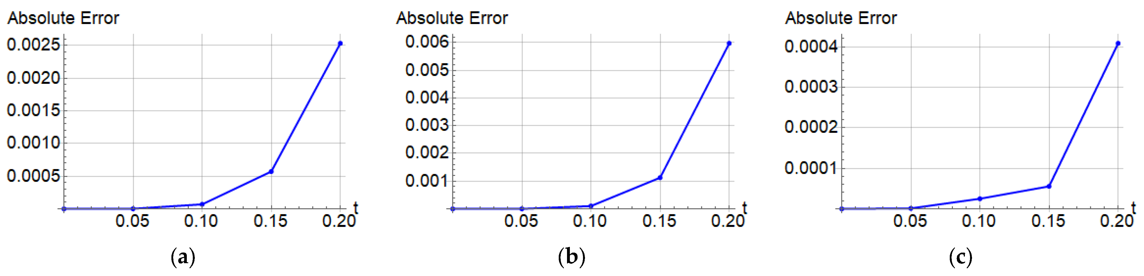
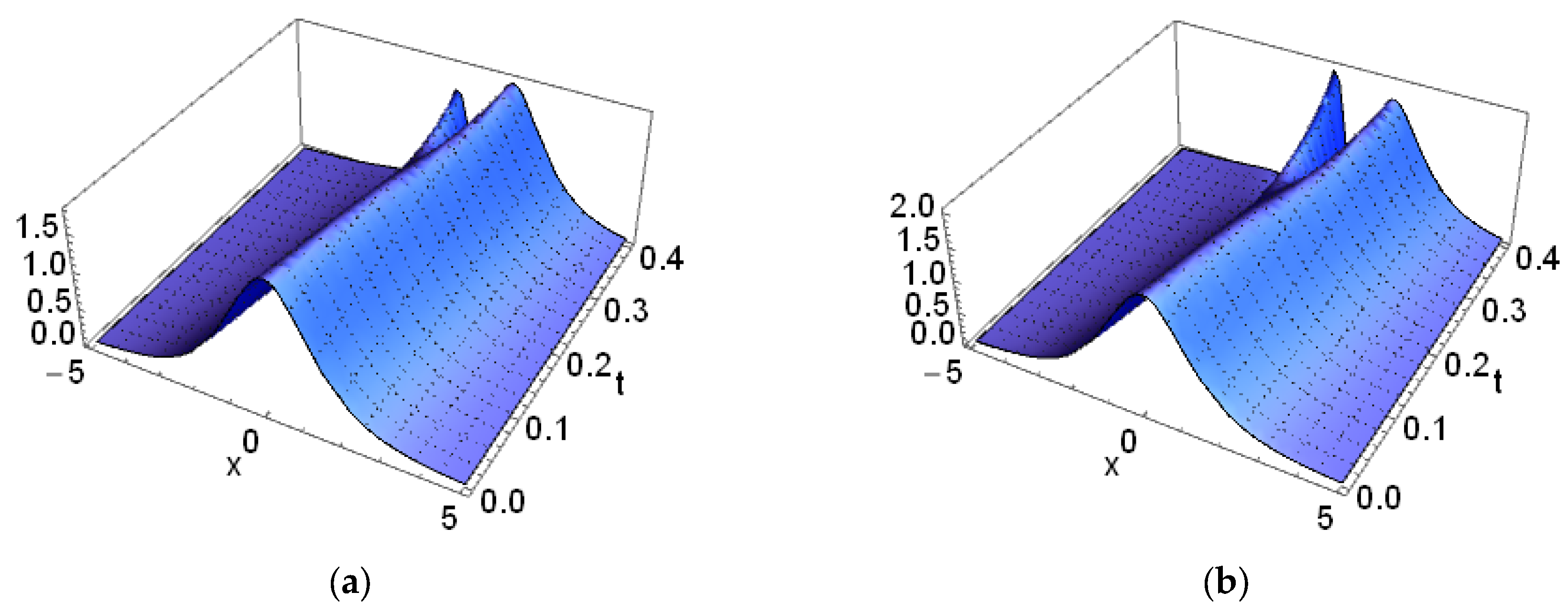
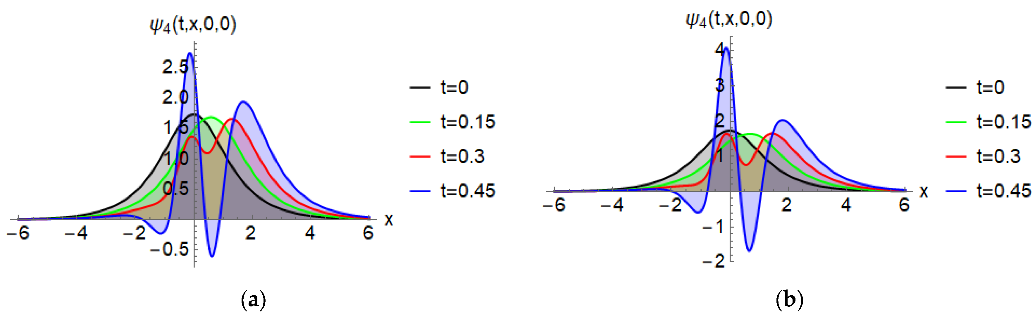
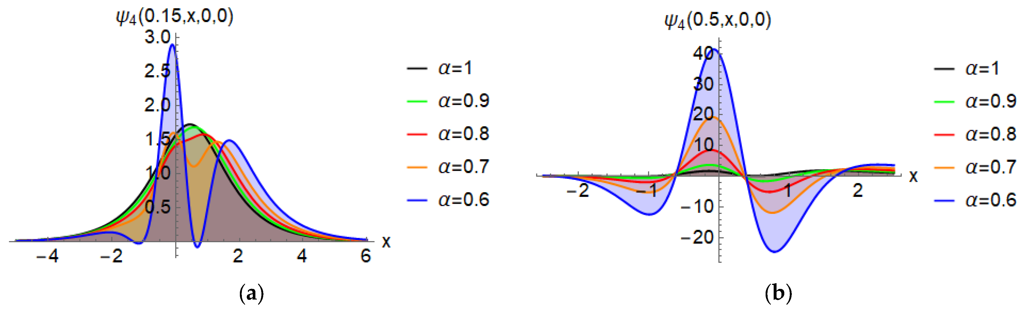
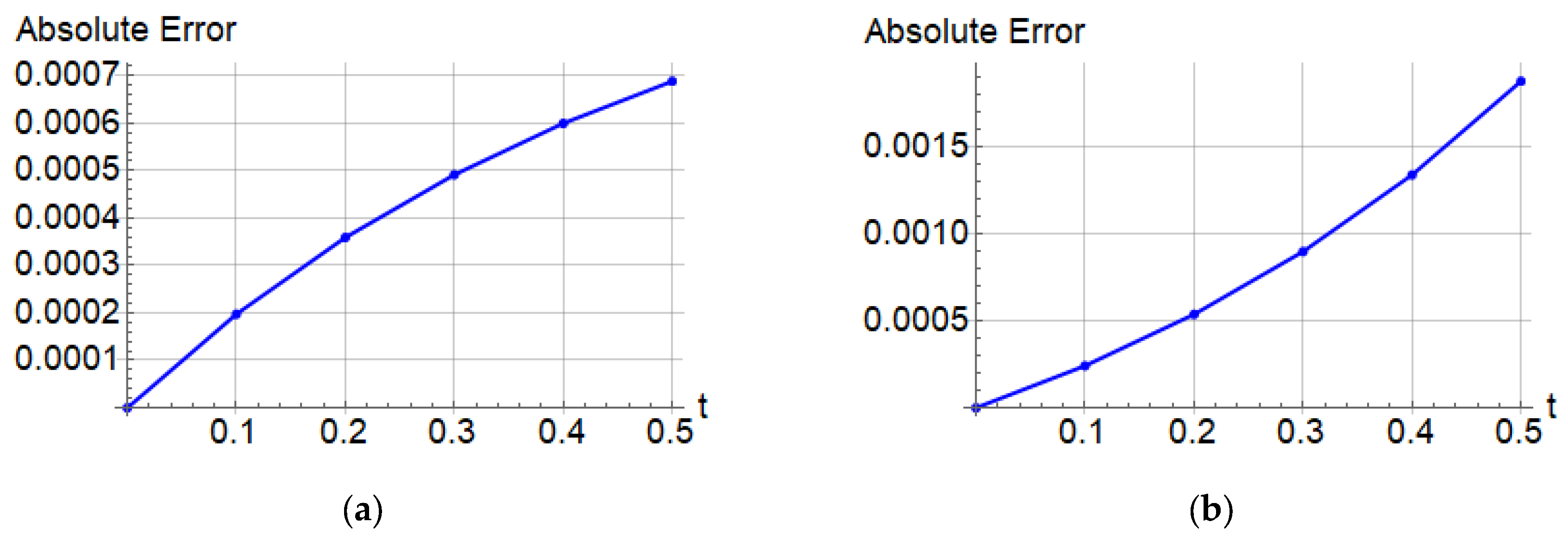
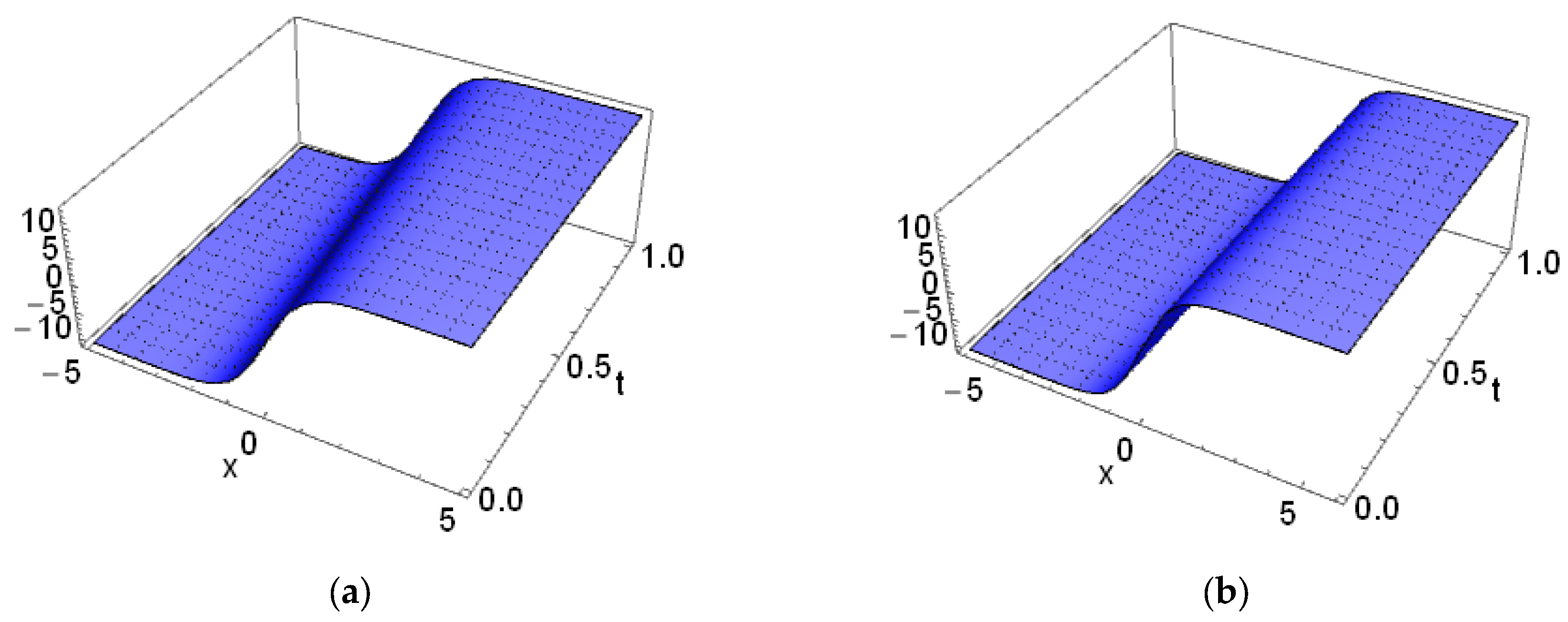
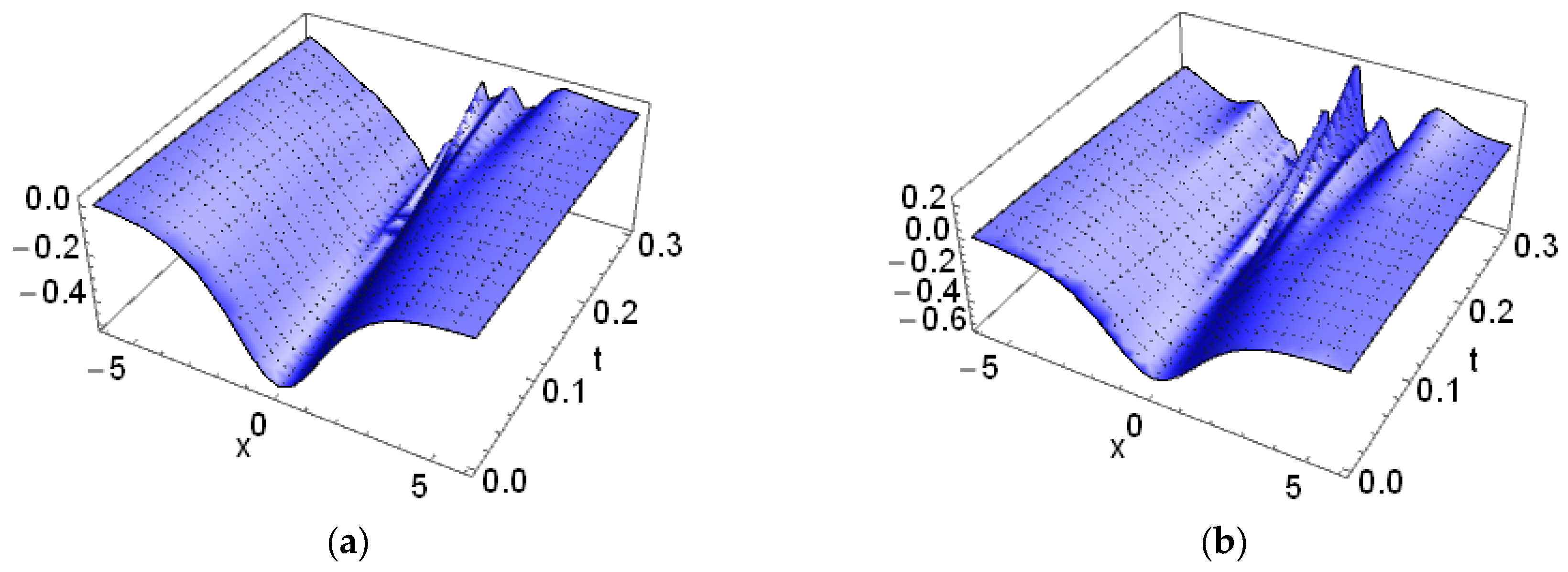
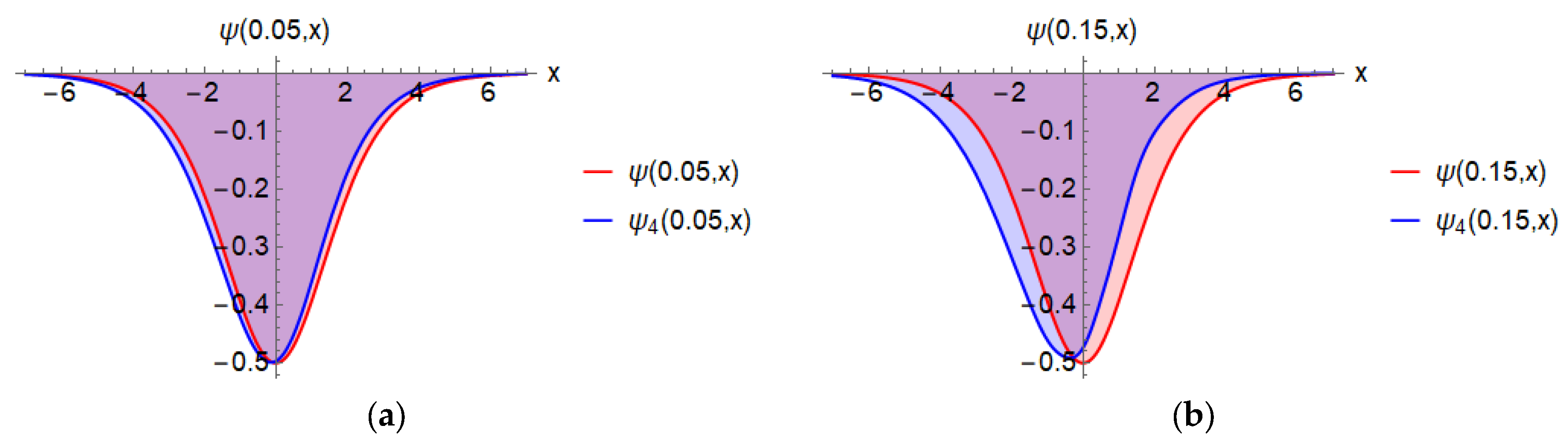
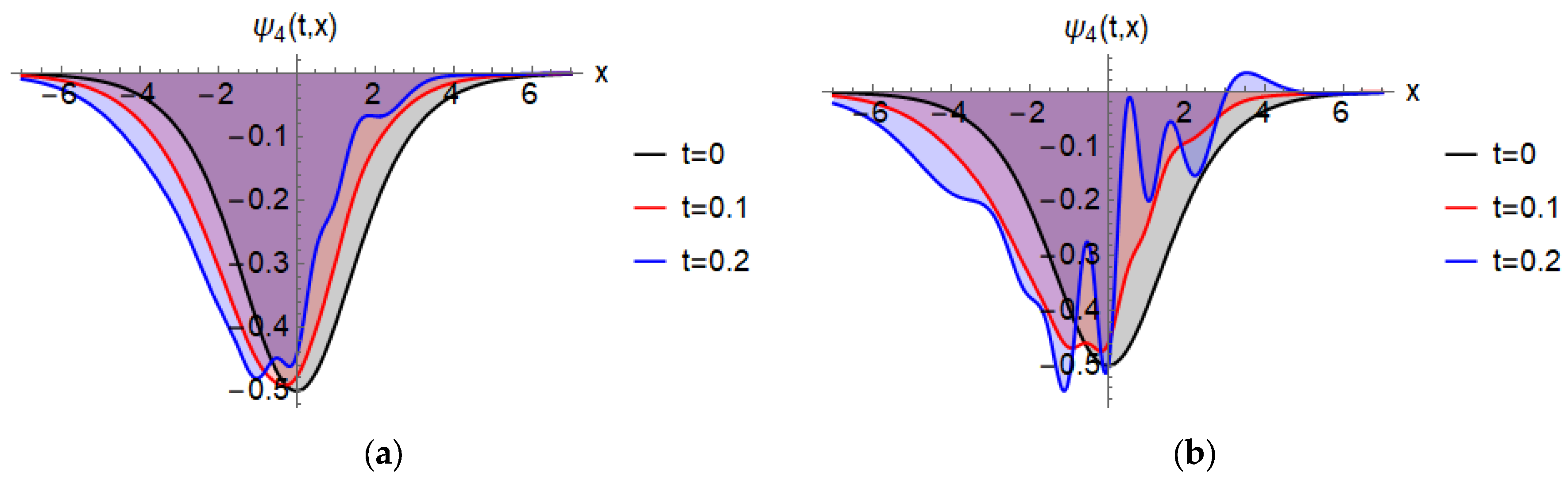
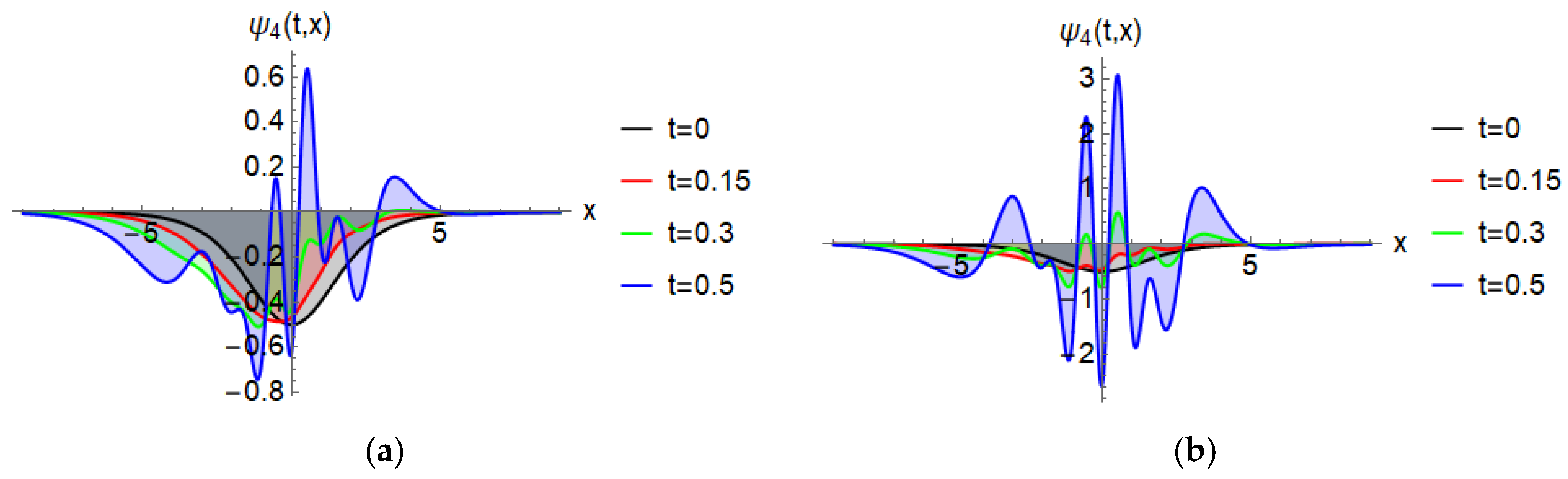
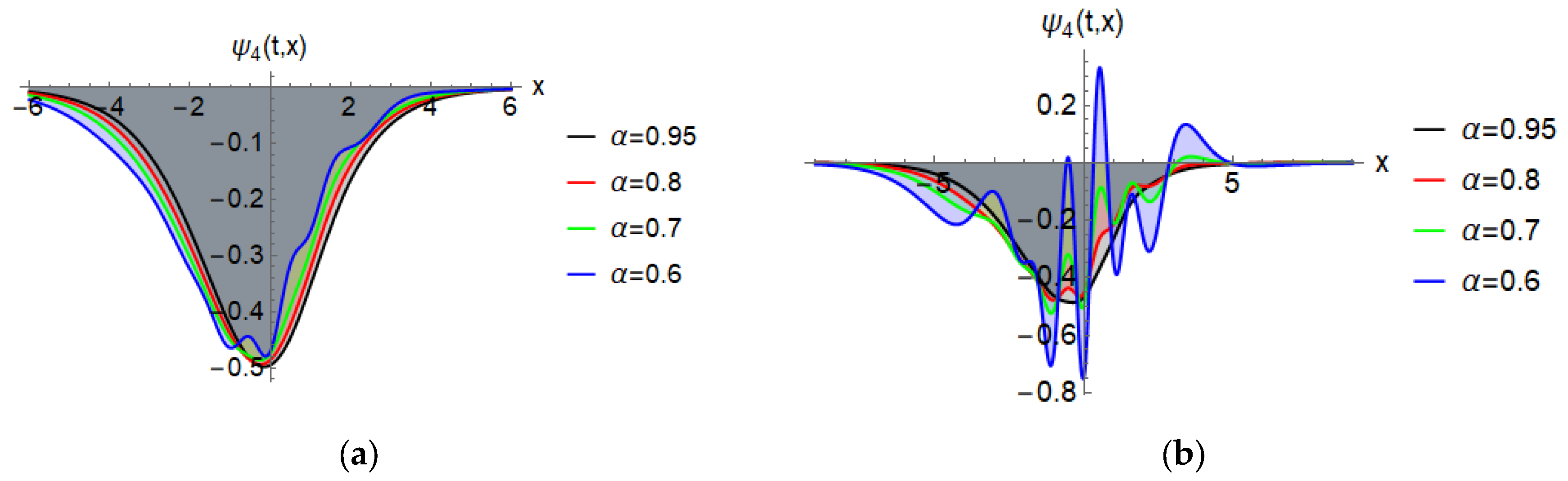
This section is devoted to presenting the NRPS method to establish approximate solutions to the nonlinear fractional PDE:

$${\mathcal{D}}_t^{\alpha }\psi \left(t,x\right)={\mathcal{G}}_x\left[\psi \left(t,x\right)\right], \alpha \in \left(0,1\right],x\in A,t\ge 0,$$

(4.1)

with the initial condition:

$$\psi \left(0,x\right)=g\left(x\right),x\in A.$$

(4.2)

The symbol ${\mathcal{G}}_x$ denotes a nonlinear operator relative to the $x$ of degree $r,x\in A,t\ge 0$, ${\mathcal{D}}_t^{\alpha }$ refers to the $\alpha$-th Caputo fractional derivative for $\alpha \in (0,1]$, and $\psi \left(t,x\right)$ is an unknown function to be determined. To obtain the desired analytical solution for (4.1)–(4.2) using the NRPS method, we can perform the following steps:

Step 1. Apply the natural transformation for both sides of (4.1) by taking advantage of the facts in Lemmas 2 and 3, we obtain:

$$\begin{gathered} \mathsf{\Psi }\left(s,w,x\right)-{\displaystyle \frac{1}{s}}g\left(x\right)-{\displaystyle \frac{w^{\alpha }}{s^{\alpha }}}\mathcal{N}\left\{{\mathcal{G}}_x\left[{\mathcal{N}}^{-1}\left\{\mathsf{\Psi }\left(s,w,x\right)\right\}\right]\right\}=0, \alpha \in \left(0,1\right],x\in A, s \\ \in \left(\theta ,\infty \right),w\in \left(0,\infty \right), \end{gathered}$$

(4.3)

where $\mathsf{\Psi }\left(s,w,x\right)=\mathcal{N}\{\psi \left(t,x\right),x\in A,s\in \left(\theta ,\mathrm{\infty }\right),w\in \left(0,\mathrm{\infty }\right)$.

Step 2. Suppose that the solution of (4.3) can be written in the following expansion:

$$\mathsf{\Psi }\left(s,w,x\right)=\sum _{k=0}^{\infty }{\displaystyle \frac{{\mathsf{\Pi }}_k\left(x\right)w^{k\alpha }}{s^{1+k\alpha }}}, \alpha \in \left(0,1\right],x\in A, s\in \left(\theta ,\infty \right),w\in \left(0,\infty \right).$$

(4.4)

Define the $\mathcal{K}$th truncated series of $\mathsf{\Psi }\left(s,w,x\right)$ as:

$${\mathsf{\Psi }}_{\mathcal{K}}\left(s,w,x\right)=\sum _{k=0}^{\mathcal{K}}{\displaystyle \frac{{\mathsf{\Pi }}_k\left(x\right)w^{k\alpha }}{s^{1+k\alpha }}}, \alpha \in \left(0,1\right],x\in A, s\in \left(\theta ,\infty \right),w\in \left(0,\infty \right).$$

(4.5)

Using the results in Theorem 2, we deduce that the initial guess ${\mathsf{\Pi }}_0\left(x\right)=g\left(x\right)$. Upon this fact, we write the $\mathcal{K}$th truncated series of $\mathsf{\Psi }\left(s,w,x\right)$ as:

$${\mathsf{\Psi }}_{\mathcal{K}}\left(s,w,x\right)={\displaystyle \frac{g\left(x\right)}{s}}+\sum _{k=1}^{\mathcal{K}}{\displaystyle \frac{{\mathsf{\Pi }}_k\left(x\right)w^{k\alpha }}{s^{1+k\alpha }}}, \alpha \in \left(0,1\right],x\in A, s\in \left(\theta ,\infty \right),w\in \left(0,\infty \right).$$

(4.6)

Step 3. We define the so-called natural residual function (NRF) as:

$$\begin{gathered} \mathcal{N}Res\left(s,w,x\right)=\mathsf{\Psi }\left(s,w,x\right)-{\displaystyle \frac{1}{s}}g\left(x\right)-{\displaystyle \frac{w^{\alpha }}{s^{\alpha }}}\mathcal{N}\left\{{\mathcal{G}}_x\left[{\mathcal{N}}^{-1}\left\{\mathsf{\Psi }\left(s,w,x\right)\right\}\right]\right\}, \alpha \\ \in \left(0,1\right],x\in A, s\in \left(\theta ,\infty \right),w\in \left(0,\infty \right), \end{gathered}$$

(4.7)

and the $\mathcal{K}$th truncated NRF as:

$$\begin{gathered} \mathcal{N}Re{s}_{\mathcal{K}}\left(s,w,x\right)={\mathsf{\Psi }}_{\mathcal{K}}\left(s,w,x\right)-{\displaystyle \frac{1}{s}}g\left(x\right)-{\displaystyle \frac{w^{\alpha }}{s^{\alpha }}}\mathcal{N}\left\{{\mathcal{G}}_x\left[{\mathcal{N}}^{-1}\left\{{\mathsf{\Psi }}_{\mathcal{K}}\left(s,w,x\right)\right\}\right]\right\}, \alpha \\ \in \left(0,1\right],x\in A, s\in \left(\theta ,\infty \right),w\in \left(0,\infty \right), \end{gathered}$$

(4.8)

Now, we introduce some essential facts to obtain the desired coefficients ${\mathsf{\Pi }}_k\left(x\right)$ in the expansion (4.6).

Remark 3.

The NRF and the $\mathcal{K}$th truncated NRF in (4.7) and (4.8), respectively, satisfy the following properties:

$$\begin{array}{}\hfill \text{(4.9)}\hfill & \hfill \text{(i)}\hfill & \mathcal{N}Res\left(s,w,x\right)=0,x\in A,s\in \left(\theta ,\mathrm{\infty }\right),w\in \left(0,\mathrm{\infty }\right).\hfill \hfill \text{(4.10)}\hfill & \hfill \text{(ii)}\hfill & \underset{k\to \infty }{\lim }\mathcal{N}Re{s}_{\mathcal{K}}\left(s,w,x\right)=\mathcal{N}Res\left(s,w,x\right),x\in A, s\in \left(\theta ,\infty \right),w\in \left(0,\infty \right).\hfill \hfill \text{(4.11)}\hfill & \hfill \text{(iii)}\hfill & \underset{s\to \infty }{\lim }{s}^{1+\mathcal{K}\alpha }\mathcal{N}Re{s}_{\mathcal{K}}\left(s,w,x\right)=0, \mathcal{K}=1,2,\dots ,x\in A, s\in \left(\theta ,\infty \right),w\in \left(0,\infty \right).\hfill \end{array}$$

Proof. 

The properties (i) and (ii) are clear. To prove (iii), we represent the NRF (4.7) in fractional expansion as:

$$\begin{gathered} \mathcal{N}Res\left(s,w,x\right)=\sum _{k=1}^{\infty }{\displaystyle \frac{\left({\mathsf{\Pi }}_k\left(x\right)-{\mathcal{G}}_x^{\left(k\right)}\left[{\mathsf{\Pi }}_i\left(x\right)\right]\right)w^{k\alpha }}{s^{1+k\alpha }}}, \alpha \in \left(0,1\right],x\in A, s\in \left(\theta ,\infty \right),w \\ \in \left(0,\infty \right), i\in \left\{0,1,2,\dots ,k-1\right\}, \end{gathered}$$

(4.12)

where ${\mathcal{G}}_x^{\left(k\right)},k=1,2,3,\dots$ are differential operators related to the $x$ of degree $r$. Using (4.9), we obtain ${\mathsf{\Pi }}_k\left(x\right)-{\mathcal{G}}_x^{\left(k\right)}\left[{\mathsf{\Pi }}_i\left(x\right)\right]=0$ for $k=1,2,3,\dots$ and $i\in \left\{0,1,2,\dots ,k-1\right\}$. Substitute the $\mathcal{K}$th truncated series ${\mathsf{\Psi }}_{\mathcal{K}}\left(s,w,x\right)$ into (4.12) that can be written in the following expression:

$$\mathcal{N}Re{s}_{\mathcal{K}}\left(s,w,x\right)=\sum _{k=1}^{\mathcal{K}}{\displaystyle \frac{\left({\mathsf{\Pi }}_k\left(x\right)-{\mathcal{G}}_x^{\left(k\right)}\left[{\mathsf{\Pi }}_i\left(x\right)\right]\right)w^{k\alpha }}{s^{1+k\alpha }}}+\sum _{k=\mathcal{K}+1}^{\mathcal{K}r+1}{\displaystyle \frac{\left({\mathsf{\Pi }}_k\left(x\right)-{{\mathcal{G}}^{*}}_x^{\left(\mathcal{K}k\right)}\left[{\mathsf{\Pi }}_j\left(x\right)\right]\right)w^{k\alpha }}{s^{1+k\alpha }}},$$

4.13

where $i\in \left\{0,1,2,\dots ,k-1\right\},j\in \left\{0,1,2,\dots ,\mathcal{K}\right\},$ and ${{\mathcal{G}}^{\mathrm{*}}}_x^{\left(\mathcal{K}k\right)},k=\mathcal{K}+1,\mathcal{K}+2,\dots ,\mathcal{K}r+1$ are differential operators related to $x$ and ${\mathsf{\Pi }}_k\left(x\right)-{{\mathcal{G}}^{\mathrm{*}}}_x^{\left(\mathcal{K}k\right)}\left[{\mathsf{\Pi }}_j\left(x\right)\right]\ne 0$. By multiplying both sides of (4.13) by $s^{1+k\alpha }$ and taking the limit as $s\to \mathrm{\infty }$, we obtain:

$$\begin{gathered} \underset{s\to \infty }{\lim }{s}^{1+k\alpha }\mathcal{N}Re{s}_k\left(s,w,x\right)=\left({\mathsf{\Pi }}_k\left(x\right)-{\mathcal{G}}_x^{\left(k\right)}\left[{\mathsf{\Pi }}_i\left(x\right)\right]\right)w^{k\alpha }=0, k=1,2,\dots ,i \\ \in \left\{0,1,2,\dots ,k-1\right\}. \end{gathered}$$

4.14

Step 4. Substitute the $\mathcal{K}$th truncated series ${\mathsf{\Psi }}_{\mathcal{K}}\left(s,w,x\right)$ in (4.6) into the $\mathcal{K}$th truncated NRF (4.8).

Step 5. To determine the coefficients ${\mathsf{\Pi }}_k\left(x\right), k=1,2,\dots ,\mathcal{K}$, we solve the system that was obtained using $\underset{s\to \infty }{\lim }{s}^{1+k\alpha }\mathcal{N}Re{s}_k\left(s,w,x\right)=0,k=1,2,\dots ,\mathcal{K}$ and collect the results into the $\mathcal{K}$th truncated series ${\mathsf{\Psi }}_{\mathcal{K}}\left(s,w,x\right)$ in (4.6).

Step 6. Apply the inverse natural operator for both sides of the inferred $\mathcal{K}$th truncated series ${\mathsf{\Psi }}_{\mathcal{K}}\left(s,w,x\right)$ to obtain the $\mathcal{K}$th approximate solution for the nonlinear fractional PDE (4.1). □

5. Applications

In this section, we investigate the time-fractional KdV-ZK Equations (1.1) and (1.2), the time-fractional spKdV Equations (1.3) and (1.4), and the fractional FKdV Equations (1.5) and (1.6) using the proposed NRPS method. We used the mathematical software package Mathematica 13 to implement all symbolic and numerical computations.

Application 1.

Consider the time-fractional KdV-ZK equation [17]:

$${\mathcal{D}}_t^{\alpha }\psi +36\psi {\displaystyle \frac{\partial \psi }{\partial x}}+{\displaystyle \frac{{\partial }^3\psi }{\partial x^3}}+{\displaystyle \frac{{\partial }^3\psi }{\partial x\partial y^2}}+{\displaystyle \frac{{\partial }^3\psi }{\partial x\partial z^2}}=0, t\ge 0, x,y,z\in \mathbb{R},$$

(5.1)

subject to the initial condition:

$$\psi \left(0,x,y,z\right)={\displaystyle \frac{1}{\sqrt{2}}}\mathrm{s}\mathrm{e}\mathrm{c}\mathrm{h}\left(x+y+z\right),x,y,z\in \mathbb{R}.$$

(5.2)

Apply the natural transformation for both sides of (5.1) with the aid of (3.13) to obtain:

$$\begin{array}{c}{\displaystyle \frac{s^{\alpha }}{w^{\alpha }}}\mathsf{\Psi }\left(s,w,x,y,z\right)-{\displaystyle \frac{s^{\alpha -1}}{w^{\alpha }}}\psi \left(0,x,y,z\right)+36\mathcal{N}\left\{{\mathcal{N}}^{-1}\left\{\mathsf{\Psi }\left(s,w,x,y,z\right)\right\}{\displaystyle \frac{\partial }{\partial x}}{\mathcal{N}}^{-1}\left\{\mathsf{\Psi }\left(s,w,x,y,z\right)\right\}\right\}\\ \begin{array}{cc} & +\mathcal{N}\left\{{\displaystyle \frac{{\partial }^3}{\partial x^3}}{\mathcal{N}}^{-1}\left\{\mathsf{\Psi }\left(s,w,x,y,z\right)\right\}\right\}+\mathcal{N}\left\{{\displaystyle \frac{{\partial }^3}{\partial x\partial y^2}}{\mathcal{N}}^{-1}\left\{\mathsf{\Psi }\left(s,w,x,y,z\right)\right\}\right\}\hfill \\ & +\mathcal{N}\left\{{\displaystyle \frac{{\partial }^3}{\partial x\partial z^2}}{\mathcal{N}}^{-1}\left\{\mathsf{\Psi }\left(s,w,x,y,z\right)\right\}\right\}=0,\hfill \end{array}\end{array}$$

(5.3)

where $\Psi \left(s,w,x,y,z\right)=\mathcal{N}\left\{\psi \left(t,x,y,z\right)\right\}$. Using (5.2) in (5.3), we obtain:

$$\begin{array}{cc}\hfill \mathsf{\Psi }\left(s,w,x,y,z\right)-& {\displaystyle \frac{1}{s\sqrt{2}}}\mathrm{s}\mathrm{e}\mathrm{c}\mathrm{h}\left(x+y+z\right)\hfill \\ & +{\displaystyle \frac{w^{\alpha }}{s^{\alpha }}}(36\mathcal{N}\left\{{\mathcal{N}}^{-1}\left\{\mathsf{\Psi }\left(s,w,x,y,z\right)\right\}{\displaystyle \frac{\partial }{\partial x}}{\mathcal{N}}^{-1}\left\{\mathsf{\Psi }\left(s,w,x,y,z\right)\right\}\right\}\hfill \\ & +\mathcal{N}\left\{{\displaystyle \frac{{\partial }^3}{\partial x^3}}{\mathcal{N}}^{-1}\left\{\mathsf{\Psi }\left(s,w,x,y,z\right)\right\}\right\}\hfill \\ & +\mathcal{N}\left\{{\displaystyle \frac{{\partial }^3}{\partial x\partial y^2}}{\mathcal{N}}^{-1}\left\{\mathsf{\Psi }\left(s,w,x,y,z\right)\right\}\right\}\hfill \\ & +\mathcal{N}\left\{{\displaystyle \frac{{\partial }^3}{\partial x\partial z^2}}{\mathcal{N}}^{-1}\left\{\mathsf{\Psi }\left(s,w,x,y,z\right)\right\}\right\})=0,\hfill \end{array}$$

(5.4)

Suppose that the solution of (5.4) can be written in the following expansion:

$$\mathsf{\Psi }\left(s,w,x,y,z\right)=\sum _{k=0}^{\infty }{\displaystyle \frac{{\mathsf{\Pi }}_k\left(x,y,z\right)w^{k\alpha }}{s^{1+k\alpha }}}, \alpha \in \left(0,1\right],x,y,z\in A, s\in \left(\theta ,\infty \right),w\in \left(0,\infty \right).$$

(5.5)

Define the $\mathcal{K}$th truncated series of $\Psi \left(s,w,x,y,z\right)$ as:

$${\mathsf{\Psi }}_{\mathcal{K}}\left(s,w,x,y,z\right)=\sum _{k=0}^{\mathcal{K}}{\displaystyle \frac{{\mathsf{\Pi }}_k\left(x,y,z\right)w^{k\alpha }}{s^{1+k\alpha }}}, \alpha \in \left(0,1\right],x,y,z\in A, s\in \left(\theta ,\infty \right),w\in \left(0,\infty \right).$$

(5.6)

Using the results in Theorem 2, we deduce that the initial guess ${\Pi }_0\left(x,y,z\right)=\sqrt{{\displaystyle \frac{1}{2}}}sech\left(\left(x+y+z\right)\right)$. Upon this fact, we write the $\mathcal{K}$th truncated series of $\Psi \left(s,w,x,y,z\right)$ as:

$${\mathsf{\Psi }}_{\mathcal{K}}\left(s,w,x,y,z\right)={\displaystyle \frac{1}{s\sqrt{2}}}\mathrm{s}\mathrm{e}\mathrm{c}\mathrm{h}\left(x+y+z\right)+\sum _{k=1}^{\mathcal{K}}{\displaystyle \frac{{\mathsf{\Pi }}_k\left(x,y,z\right)w^{k\alpha }}{s^{1+k\alpha }}}.$$

(5.7)

We define the NRF as:

$$\begin{array}{cc}\hfill \mathcal{N}Res\left(s,w,x,y,z\right)& \\ & =\mathsf{\Psi }\left(s,w,x,y,z\right)-{\displaystyle \frac{1}{s\sqrt{2}}}\mathrm{s}\mathrm{e}\mathrm{c}\mathrm{h}\left(x+y+z\right)\hfill \\ & +{\displaystyle \frac{w^{\alpha }}{s^{\alpha }}}(36\mathcal{N}\left\{{\mathcal{N}}^{-1}\left\{\mathsf{\Psi }\left(s,w,x,y,z\right)\right\}{\displaystyle \frac{\partial }{\partial x}}{\mathcal{N}}^{-1}\left\{\mathsf{\Psi }\left(s,w,x,y,z\right)\right\}\right\}\hfill \\ & +\mathcal{N}\left\{{\displaystyle \frac{{\partial }^3}{\partial x^3}}{\mathcal{N}}^{-1}\left\{\mathsf{\Psi }\left(s,w,x,y,z\right)\right\}\right\}\hfill \\ & +\mathcal{N}\left\{{\displaystyle \frac{{\partial }^3}{\partial x\partial y^2}}{\mathcal{N}}^{-1}\left\{\mathsf{\Psi }\left(s,w,x,y,z\right)\right\}\right\}\hfill \\ & +\mathcal{N}\left\{{\displaystyle \frac{{\partial }^3}{\partial x\partial z^2}}{\mathcal{N}}^{-1}\left\{\mathsf{\Psi }\left(s,w,x,y,z\right)\right\}\right\}),\hfill \end{array}$$

(5.8)

and the $\mathcal{K}$th truncated NRF as:

$$\begin{array}{cc}\hfill \mathcal{N}Re{s}_{\mathcal{K}}\left(s,w,x,y,z\right)& \\ & ={\mathsf{\Psi }}_{\mathcal{K}}\left(s,w,x,y,z\right)-{\displaystyle \frac{1}{s\sqrt{2}}}\mathrm{s}\mathrm{e}\mathrm{c}\mathrm{h}\left(x+y+z\right)\hfill \\ & +{\displaystyle \frac{w^{\alpha }}{s^{\alpha }}}(36\mathcal{N}\left\{{\mathcal{N}}^{-1}\left\{{\mathsf{\Psi }}_{\mathcal{K}}\left(s,w,x,y,z\right)\right\}{\displaystyle \frac{\partial }{\partial x}}{\mathcal{N}}^{-1}\left\{{\mathsf{\Psi }}_{\mathcal{K}}\left(s,w,x,y,z\right)\right\}\right\}\hfill \\ & +\mathcal{N}\left\{{\displaystyle \frac{{\partial }^3}{\partial x^3}}{\mathcal{N}}^{-1}\left\{{\mathsf{\Psi }}_{\mathcal{K}}\left(s,w,x,y,z\right)\right\}\right\}\hfill \\ & +\mathcal{N}\left\{{\displaystyle \frac{{\partial }^3}{\partial x\partial y^2}}{\mathcal{N}}^{-1}\left\{{\mathsf{\Psi }}_{\mathcal{K}}\left(s,w,x,y,z\right)\right\}\right\}\hfill \\ & +\mathcal{N}\left\{{\displaystyle \frac{{\partial }^3}{\partial x\partial z^2}}{\mathcal{N}}^{-1}\left\{{\mathsf{\Psi }}_{\mathcal{K}}\left(s,w,x,y,z\right)\right\}\right\}).\hfill \end{array}$$

(5.9)

For $\mathcal{K}=1$, we obtain the 1st NRF with using (5.7) as follows:

$$\begin{array}{cc}\hfill \mathcal{N}Re{s}_1\left(s,w,x,y,z\right)& \\ & ={\displaystyle \frac{{\mathsf{\Pi }}_1\left(x,y,z\right)w^{\alpha }}{s^{1+\alpha }}}\hfill \\ & +{\displaystyle \frac{w^{\alpha }}{s^{\alpha }}}\left(36\mathcal{N}\right\{{\mathcal{N}}^{-1}\left\{{\displaystyle \frac{1}{s\sqrt{2}}}\mathrm{s}\mathrm{e}\mathrm{c}\mathrm{h}\left(x+y+z\right)+{\displaystyle \frac{{\mathsf{\Pi }}_1\left(x,y,z\right)w^{\alpha }}{s^{1+\alpha }}}\right\}{\displaystyle \frac{\partial }{\partial x}}{\mathcal{N}}^{-1}\{{\displaystyle \frac{1}{s\sqrt{2}}}\mathrm{s}\mathrm{e}\mathrm{c}\mathrm{h}\left(x+y+z\right)\hfill \\ & +{\displaystyle \frac{{\mathsf{\Pi }}_1\left(x,y,z\right)w^{\alpha }}{s^{1+\alpha }}}\left\}\right\}+\mathcal{N}\left\{{\displaystyle \frac{{\partial }^3}{\partial x^3}}{\mathcal{N}}^{-1}\left\{{\displaystyle \frac{1}{s\sqrt{2}}}\mathrm{s}\mathrm{e}\mathrm{c}\mathrm{h}\left(x+y+z\right)+{\displaystyle \frac{{\mathsf{\Pi }}_1\left(x,y,z\right)w^{\alpha }}{s^{1+\alpha }}}\right\}\right\}\hfill \\ & +\mathcal{N}\left\{{\displaystyle \frac{{\partial }^3}{\partial x\partial y^2}}{\mathcal{N}}^{-1}\left\{{\displaystyle \frac{1}{s\sqrt{2}}}\mathrm{s}\mathrm{e}\mathrm{c}\mathrm{h}\left(x+y+z\right)+{\displaystyle \frac{{\mathsf{\Pi }}_1\left(x,y,z\right)w^{\alpha }}{s^{1+\alpha }}}\right\}\right\}\hfill \\ & +\mathcal{N}\left\{{\displaystyle \frac{{\partial }^3}{\partial x\partial z^2}}{\mathcal{N}}^{-1}\right\{{\displaystyle \frac{1}{s\sqrt{2}}}\mathrm{s}\mathrm{e}\mathrm{c}\mathrm{h}\left(x+y+z\right)+{\displaystyle \frac{{\mathsf{\Pi }}_1\left(x,y,z\right)w^{\alpha }}{s^{1+\alpha }}}\left\}\right\}).\hfill \end{array}$$

(5.10)

By multiplying both sides of (5.10) by $s^{1+\alpha }$ and using $\underset{s\to \infty }{\mathit{lim}}{s}^{1+\alpha }\mathcal{N}Re{s}_1\left(s,w,x\right)=0$, we obtain:

$${\mathsf{\Pi }}_1\left(x,y,z\right)=3\sqrt{3}\mathrm{sech}\left(x+y+z\right)\tanh \left(x+y+z\right).$$

(5.11)

Similarly, we can obtain the following:

$${\mathsf{\Pi }}_2\left(x,y,z\right)={\displaystyle \frac{9}{2}}\sqrt{3}\left(-3+\cosh \left(2\left(x+y+z\right)\right)\right){\mathrm{sech}\left(x+y+z\right)}^3.$$

(5.12)

$${\mathsf{\Pi }}_3\left(x,y,z\right)={\displaystyle \frac{27}{4}}\sqrt{3}{\mathrm{sech}\left(x+y+z\right)}^4\left(-23\sinh \left(x+y+z\right)+\sinh \left(3\left(x+y+z\right)\right)\right).$$

(5.13)

$${\mathsf{\Pi }}_4\left(x,y,z\right)={\displaystyle \frac{81\sqrt{3}}{8}}\left(115-76\cosh \left(2\left(x+y+z\right)\right)+\cosh \left(4\left(x+y+z\right)\right)\right){\mathrm{sech}\left(x+y+z\right)}^5.$$

(5.14)

The CPU time that is needed to obtain these results (5.11)–(5.14) was $35.390625$ s. Substitute (5.11)–(5.14) into (5.7) to obtain the $\mathcal{K}$th truncated series of $\Psi \left(s,w,x\right)$ as:

$$\begin{gathered} {\mathsf{\Psi }}_{\mathcal{K}}\left(s,w,x,y,z\right)={\displaystyle \frac{1}{s\sqrt{2}}}\mathrm{s}\mathrm{e}\mathrm{c}\mathrm{h}\left(x+y+z\right)+{\displaystyle \frac{{\mathsf{\Pi }}_1\left(x,y,z\right)w^{\alpha }}{s^{1+\alpha }}}+{\displaystyle \frac{{\mathsf{\Pi }}_2\left(x,y,z\right)w^{2\alpha }}{s^{1+2\alpha }}} \\ +{\displaystyle \frac{{\mathsf{\Pi }}_3\left(x,y,z\right)w^{3\alpha }}{s^{1+3\alpha }}}+{\displaystyle \frac{{\mathsf{\Pi }}_4\left(x,y,z\right)w^{4\alpha }}{s^{1+4\alpha }}}+\dots +{\displaystyle \frac{{\mathsf{\Pi }}_{\mathcal{K}}\left(x,y,z\right)w^{\mathcal{K}\alpha }}{s^{1+\mathcal{K}\alpha }}}. \end{gathered}$$

(5.15)

Apply the inverse natural operator of (5.15) to obtain the $\mathcal{K}$th NRPS solution for the time-fractional KdV-ZK equation as:

$$\begin{gathered} {\psi }_{\mathcal{K}}\left(t,x,y,z\right)={\displaystyle \frac{1}{\sqrt{2}}}\mathrm{s}\mathrm{e}\mathrm{c}\mathrm{h}\left(x+y+z\right)+{\displaystyle \frac{{\mathsf{\Pi }}_1\left(x,y,z\right)t^{\alpha }}{\mathsf{\Gamma }\left(1+\alpha \right)}}+{\displaystyle \frac{{\mathsf{\Pi }}_2\left(x,y,z\right)t^{2\alpha }}{\mathsf{\Gamma }\left(1+2\alpha \right)}} \\ +{\displaystyle \frac{{\mathsf{\Pi }}_3\left(x,y,z\right)t^{3\alpha }}{\mathsf{\Gamma }\left(1+3\alpha \right)}}+{\displaystyle \frac{{\mathsf{\Pi }}_4\left(x,y,z\right)t^{4\alpha }}{\mathsf{\Gamma }\left(1+4\alpha \right)}}+\dots +{\displaystyle \frac{{\mathsf{\Pi }}_{\mathcal{K}}\left(x,y,z\right)t^{\mathcal{K}\alpha }}{\mathsf{\Gamma }\left(1+\mathcal{K}\alpha \right)}}. \end{gathered}$$

(5.16)

We present a numerical simulation of the results obtained. We assume that $y=z=0$.

Table 1. A comparison between the exact solution and the NRPS solution for the time-fractional KdV-ZK equation.

$$\mathit{x}$$	$$\mathit{t}$$	Exact Solution	NRPS Solution	Absolute Error	Relative Error	CPU Time
$-1$	$\begin{array}{c}0.0\\ 0.1\\ 0.2\\ 0.3\end{array}$	$\begin{array}{c}1.122462928047994\\ 0.878805774963547\\ 0.671997937091220\\ 0.506783751732631\end{array}$	$\begin{array}{c}1.122462928047995\\ 0.878736016940593\\ 0.669464247695219\\ 0.486544390701797\end{array}$	$\begin{array}{c}2.220446\times {10}^{-16}\\ 6.975802\times {10}^{-5}\\ 2.533689\times {10}^{-3}\\ 2.023936\times {10}^{-2}\end{array}$	$\begin{array}{c}1.978190\times {10}^{-16}\\ 7.937820\times {10}^{-5}\\ 3.770382\times {10}^{-3}\\ 3.993687\times {10}^{-2}\end{array}$	$0.015625$
$0$	$\begin{array}{c}0.0\\ 0.1\\ 0.2\\ 0.3\end{array}$	$\begin{array}{c}1.732050807568877\\ 1.656928147349753\\ 1.461072649720631\\ 1.208615771635065\end{array}$	$\begin{array}{c}1.732050807568877\\ 1.657031356966050\\ 1.467047034010839\\ 1.267319925263052\end{array}$	$\begin{array}{c}2.220446\times {10}^{-16}\\ 1.032096\times {10}^{-5}\\ 5.974384\times {10}^{-3}\\ 5.870415\times {10}^{-2}\end{array}$	$\begin{array}{c}1.281975\times {10}^{-16}\\ 6.228973\times {10}^{-5}\\ 4.089039\times {10}^{-3}\\ 4.857139\times {10}^{-2}\end{array}$	$0.015625$
$1$	$\begin{array}{c}0.0\\ 0.1\\ 0.2\\ 0.3\end{array}$	$\begin{array}{c}1.122462928047994\\ 1.379934335375192\\ 1.602159904080592\\ 1.723426491772224\end{array}$	$\begin{array}{c}1.122462928047995\\ 1.379959423861089\\ 1.601751160457130\\ 1.709575007146963\end{array}$	$\begin{array}{c}2.220446\times {10}^{-16}\\ 2.508848\times {10}^{-5}\\ 4.087436\times {10}^{-4}\\ 1.385148\times {10}^{-2}\end{array}$	$\begin{array}{c}1.978190\times {10}^{-16}\\ 1.818092\times {10}^{-5}\\ 2.551203\times {10}^{-4}\\ 8.037177\times {10}^{-3}\end{array}$	$0.015625$

compares the exact solution for the time-fractional KdV-ZK Equation (5.1) and the inferred fourth NRPS solution (5.16) where the absolute and relative errors are presented. Figure 1 presents the absolute error between the exact solution and the explored approximate fourth NRPS solution (5.16) for the time-fractional KdV-ZK Equation (5.1). To our knowledge, no works in the literature have been presented to deduce approximate solutions to Equation (5.1). Still, all the works presented are concerned with deriving exact solutions to the equation. From Table 1 and Figure 1, we can see the convergence of the numerical solutions derived through the proposed method with the exact solutions, which provides insight into the high accuracy of the proposed method. Figure 2 shows the surfaces of the exact and the fourth NRPS solutions (5.16) at $\alpha =1$. Figure 3 presents the fourth NRPS solution (5.16) surfaces at different fractional orders $\alpha =0.95$ and $\alpha =0.9$ to demonstrate the effect of the fractional derivative on the established surfaces. For more explanation, we depicted, in Figure 4, Figure 5 and Figure 6, the NRPS solutions explored in 2D plots at different fractional orders $\alpha$ where the time $t$ is considered at various values.

Applications 2.

Consider the following time-fractional spKdV equation:

$${\mathcal{D}}_t^{\alpha }\psi -8{\displaystyle \frac{\partial \psi }{\partial x}}+{\left({\displaystyle \frac{\partial \psi }{\partial x}}\right)}^2+2{\displaystyle \frac{{\partial }^3\psi }{\partial x^3}}=0, t\ge 0, x\in \mathbb{R},$$

(5.17)

subject to the initial condition:

$$\psi \left(x,0\right)=g\left(x\right)=1+12\tanh \left(x\right),x\in \mathbb{R}.$$

(5.18)

Apply the natural transformation for both sides of (5.17) with the aid of (3.13) to obtain:

$$\begin{gathered} {\displaystyle \frac{s^{\alpha }}{w^{\alpha }}}\mathsf{\Psi }\left(s,w,x\right)-{\displaystyle \frac{s^{\alpha -1}}{w^{\alpha }}}\psi \left(0,x\right)-8\mathcal{N}\left\{{\displaystyle \frac{\partial }{\partial x}}{\mathcal{N}}^{-1}\left\{\mathsf{\Psi }\left(s,w,x\right)\right\}\right\}+\mathcal{N}\left\{{\left({\displaystyle \frac{\partial }{\partial x}}{\mathcal{N}}^{-1}\left\{\mathsf{\Psi }\left(s,w,x\right)\right\}\right)}^2\right\} \\ +2\mathcal{N}\left\{{\displaystyle \frac{{\partial }^3}{\partial x^3}}{\mathcal{N}}^{-1}\left\{\mathsf{\Psi }\left(s,w,x\right)\right\}\right\}=0, \end{gathered}$$

(5.19)

where $\Psi \left(s,w,x\right)=\mathcal{N}\left\{\psi \left(t,x\right)\right\}$. Using (5.18) in (5.19), we obtain:

$$\begin{array}{cc}\hfill \mathsf{\Psi }\left(s,w,x\right)-{\displaystyle \frac{1}{s}}(1& +12\tanh \left(x\right))\hfill \\ & +{\displaystyle \frac{w^{\alpha }}{s^{\alpha }}}(-8\mathcal{N}\left\{{\displaystyle \frac{\partial }{\partial x}}{\mathcal{N}}^{-1}\left\{\mathsf{\Psi }\left(s,w,x\right)\right\}\right\}+\mathcal{N}\left\{{\left({\displaystyle \frac{\partial }{\partial x}}{\mathcal{N}}^{-1}\left\{\mathsf{\Psi }\left(s,w,x\right)\right\}\right)}^2\right\}\hfill \\ & +2\mathcal{N}\left\{{\displaystyle \frac{{\partial }^3}{\partial x^3}}{\mathcal{N}}^{-1}\left\{\mathsf{\Psi }\left(s,w,x\right)\right\}\right\})=0,\hfill \end{array}$$

(5.20)

Suppose that the solution of (5.20) can be written in the following expansion:

$$\mathsf{\Psi }\left(s,w,x\right)=\sum _{k=0}^{\infty }{\displaystyle \frac{{\mathsf{\Pi }}_k\left(x\right)w^{k\alpha }}{s^{1+k\alpha }}}, \alpha \in \left(0,1\right],x\in A, s\in \left(\theta ,\infty \right),w\in \left(0,\infty \right).$$

(5.21)

Define the $\mathcal{K}$th truncated series of $\Psi \left(s,w,x\right)$ as:

$${\mathsf{\Psi }}_{\mathcal{K}}\left(s,w,x\right)=\sum _{k=0}^{\mathcal{K}}{\displaystyle \frac{{\mathsf{\Pi }}_k\left(x\right)w^{k\alpha }}{s^{1+k\alpha }}}, \alpha \in \left(0,1\right],x\in A, s\in \left(\theta ,\infty \right),w\in \left(0,\infty \right).$$

(5.22)

Using the results in Theorem 2, we deduce that the initial guess ${\Pi }_0\left(x\right)=1+12\mathit{tanh}\left(x\right)$. Based on this fact, we write the $\mathcal{K}$th truncated series of $\Psi \left(s,w,x\right)$ as:

$${\mathsf{\Psi }}_{\mathcal{K}}\left(s,w,x\right)={\displaystyle \frac{1}{s}}\left(1+12\tanh \left(x\right)\right)+\sum _{k=1}^{\mathcal{K}}{\displaystyle \frac{{\mathsf{\Pi }}_k\left(x\right)w^{k\alpha }}{s^{1+k\alpha }}}.$$

(5.23)

We define the NRF as:

$$\begin{array}{cc}\hfill \mathcal{N}Res\left(s,w,x\right)=& \mathsf{\Psi }\left(s,w,x\right)-{\displaystyle \frac{1}{s}}\left(1+12\tanh \left(x\right)\right)\hfill \\ & +{\displaystyle \frac{w^{\alpha }}{s^{\alpha }}}(-8\mathcal{N}\left\{{\displaystyle \frac{\partial }{\partial x}}{\mathcal{N}}^{-1}\left\{\mathsf{\Psi }\left(s,w,x\right)\right\}\right\}+\mathcal{N}\left\{{\left({\displaystyle \frac{\partial }{\partial x}}{\mathcal{N}}^{-1}\left\{\mathsf{\Psi }\left(s,w,x\right)\right\}\right)}^2\right\}\hfill \\ & +2\mathcal{N}\left\{{\displaystyle \frac{{\partial }^3}{\partial x^3}}{\mathcal{N}}^{-1}\left\{\mathsf{\Psi }\left(s,w,x\right)\right\}\right\},\hfill \end{array}$$

(5.24)

and the $\mathcal{K}$th truncated NRF as:

$$\begin{array}{cc}\hfill \mathcal{N}Re{s}_{\mathcal{K}}\left(s,w,x\right)& ={\mathsf{\Psi }}_{\mathcal{K}}\left(s,w,x\right)-{\displaystyle \frac{1}{s}}\left(1+12\tanh \left(x\right)\right)\hfill \\ & +{\displaystyle \frac{w^{\alpha }}{s^{\alpha }}}(-8\mathcal{N}\left\{{\displaystyle \frac{\partial }{\partial x}}{\mathcal{N}}^{-1}\left\{{\mathsf{\Psi }}_{\mathcal{K}}\left(s,w,x\right)\right\}\right\}+\mathcal{N}\left\{{\left({\displaystyle \frac{\partial }{\partial x}}{\mathcal{N}}^{-1}\left\{{\mathsf{\Psi }}_{\mathcal{K}}\left(s,w,x\right)\right\}\right)}^2\right\}\hfill \\ & +2\mathcal{N}\left\{{\displaystyle \frac{{\partial }^3}{\partial x^3}}{\mathcal{N}}^{-1}\left\{{\mathsf{\Psi }}_{\mathcal{K}}\left(s,w,x\right)\right\}\right\},\hfill \end{array}$$

(5.25)

Using the fact that $\underset{s\to \infty }{\mathit{lim}}{s}^{1+k\alpha }\mathcal{N}Re{s}_k\left(s,w,x\right)=0, k=1,2,\dots$, we obtain:

$${\mathsf{\Pi }}_1\left(x\right)=8g^{\prime }\left(x\right)-{\left(g^{\prime }\left(x\right)\right)}^2-2g^{\prime \prime \prime }\left(x\right).$$

(5.26)

$${\mathsf{\Pi }}_2\left(x\right)=8{\mathsf{\Pi }}_1^{\prime }\left(x\right)-2g^{\prime }\left(x\right){\mathsf{\Pi }}_1^{\prime }\left(x\right)-2{\mathsf{\Pi }}_1^{\prime \prime \prime }\left(x\right).$$

(5.27)

$${\mathsf{\Pi }}_3\left(x\right)={\displaystyle \frac{-\mathsf{\Gamma }\left(1+2\alpha \right){\left({\mathsf{\Pi }}_1^{\prime }\left(x\right)\right)}^2-{\left(\mathsf{\Gamma }\left(1+\alpha \right)\right)}^2\left(-8{\mathsf{\Pi }}_2^{\prime }\left(x\right)+2g^{\prime }\left(x\right){\mathsf{\Pi }}_2^{\prime }\left(x\right)+2{\mathsf{\Pi }}_2^{\prime \prime \prime }\left(x\right)\right)}{{\left(\mathsf{\Gamma }\left(1+\alpha \right)\right)}^2}}.$$

(5.28)

$${\mathsf{\Pi }}_4\left(x\right)={\displaystyle \frac{-2\mathsf{\Gamma }\left(1+3\alpha \right){\mathsf{\Pi }}_1^{\prime }\left(x\right){\mathsf{\Pi }}_2^{\prime }\left(x\right)+8\mathsf{\Gamma }\left(1+\alpha \right)\mathsf{\Gamma }\left(1+2\alpha \right)\left(-8{\mathsf{\Pi }}_3^{\prime }\left(x\right)+2g^{\prime }\left(x\right){\mathsf{\Pi }}_3^{\prime }\left(x\right)+2{\mathsf{\Pi }}_3^{\prime \prime \prime }\left(x\right)\right)}{\mathsf{\Gamma }\left(1+\alpha \right)\mathsf{\Gamma }\left(1+2\alpha \right)}}.$$

(5.29)

The CPU time needed to obtain these results (5.26)–(5.29) was $8.53125$ s. Substitute (5.26)–(5.29) into (5.23) to obtain the $\mathcal{K}$th truncated series of $\Psi \left(s,w,x\right)$ as:

$${\mathsf{\Psi }}_{\mathcal{K}}\left(s,w,x\right)={\displaystyle \frac{1}{s}}\left(1+12\tanh \left(x\right)\right)+{\displaystyle \frac{{\mathsf{\Pi }}_1\left(x\right)w^{\alpha }}{s^{1+\alpha }}}+{\displaystyle \frac{{\mathsf{\Pi }}_2\left(x\right)w^{2\alpha }}{s^{1+2\alpha }}}+{\displaystyle \frac{{\mathsf{\Pi }}_3\left(x\right)w^{3\alpha }}{s^{1+3\alpha }}}+{\displaystyle \frac{{\mathsf{\Pi }}_4\left(x\right)w^{4\alpha }}{s^{1+4\alpha }}}+\dots +{\displaystyle \frac{{\mathsf{\Pi }}_{\mathcal{K}}\left(x\right)w^{\mathcal{K}\alpha }}{s^{1+\mathcal{K}\alpha }}}.$$

(5.30)

Apply the inverse natural operator of (5.30) to obtain the $\mathcal{K}$th NRPS solution for the time-fractional spKdV equation as:

$${\psi }_{\mathcal{K}}\left(t,x,y,z\right)=1+12\tanh \left(x\right)+{\displaystyle \frac{{\mathsf{\Pi }}_1\left(x\right)t^{\alpha }}{\mathsf{\Gamma }\left(1+\alpha \right)}}+{\displaystyle \frac{{\mathsf{\Pi }}_2\left(x\right)t^{2\alpha }}{\mathsf{\Gamma }\left(1+2\alpha \right)}}+{\displaystyle \frac{{\mathsf{\Pi }}_3\left(x\right)t^{3\alpha }}{\mathsf{\Gamma }\left(1+3\alpha \right)}}+{\displaystyle \frac{{\mathsf{\Pi }}_4\left(x\right)t^{4\alpha }}{\mathsf{\Gamma }\left(1+4\alpha \right)}}+\dots +{\displaystyle \frac{{\mathsf{\Pi }}_{\mathcal{K}}\left(x\right)t^{\mathcal{K}\alpha }}{\mathsf{\Gamma }\left(1+\mathcal{K}\alpha \right)}}.$$

(5.31)

Table 2. Comparison between the exact solution and NRPS solution for the time-fractional spKdV equation.

$\mathit{x}$	$\mathit{t}$	Exact Solution	NRPS Solution	Absolute Error	Relative Error	CPU Time
$-5$	$\begin{array}{c}0.0\\ 0.1\\ 0.2\\ 0.3\\ 0.4\\ 0.5\end{array}$	$\begin{array}{c}-10.99891045115114\\ -10.99866923540665\\ -10.99837462040912\\ -10.99801478665156\\ -10.99757529934621\\ -10.99703853017633\end{array}$	$\begin{array}{c}-10.998910451151142\\ -10.998910451151142\\ -10.998910451151142\\ -10.998910451151142\\ -10.998910451151142\\ -10.998910451151142\end{array}$	$\begin{array}{c}0.0\\ 2.412157\times {10}^{-4}\\ 5.358307\times {10}^{-4}\\ 8.956644\times {10}^{-4}\\ 1.335151\times {10}^{-3}\\ 1.871920\times {10}^{-3}\end{array}$	$\begin{array}{c}0.0\\ 2.193135\times {10}^{-5}\\ 4.871908\times {10}^{-5}\\ 8.143874\times {10}^{-5}\\ 1.214041\times {10}^{-4}\\ 1.702204\times {10}^{-4}\end{array}$	$2.328125$
$5$	$\begin{array}{c}0.0\\ 0.1\\ 0.2\\ 0.3\\ 0.4\\ 0.5\end{array}$	$\begin{array}{c}12.99891045115114\\ 12.99910794550953\\ 12.99926964263438\\ 12.99940203066545\\ 12.99951042190528\\ 12.99959916587564\end{array}$	$\begin{array}{c}12.998910451151142\\ 12.998910451151142\\ 12.998910451151142\\ 12.998910451151142\\ 12.998910451151142\\ 12.998910451151142\end{array}$	$\begin{array}{c}0.0\\ 1.974943\times {10}^{-4}\\ 3.591914\times {10}^{-4}\\ 4.915795\times {10}^{-4}\\ 5.999707\times {10}^{-4}\\ 6.887147\times {10}^{-4}\end{array}$	$\begin{array}{c}0.0\\ 1.519291\times {10}^{-5}\\ 2.763166\times {10}^{-5}\\ 3.781554\times {10}^{-5}\\ 4.615333\times {10}^{-5}\\ 5.297968\times {10}^{-5}\end{array}$	$1.703125$

shows the absolute and relative errors for the constructed numerical results to demonstrate the accuracy of the NRPS method. Figure 7 presents the absolute error between the exact solution and the explored approximate 4th NRPS solution (5.31) for the time-fractional spKdV Equation (5.17). When comparing the solution explored using the proposed method and the exact solution and calculating the absolute error and relative error, it becomes clear that the proposed method achieves an accuracy within ${10}^{-4}$ in dealing with Equation (5.17), which is a suitable level for numerical modeling applications that require accurate and stable solutions. It is worth noting here that based on the literature review, it was found that there are no works that focused on extracting approximate solutions to Equation (5.17), which prompted us to compare the approximate solutions derived here with the exact solutions to the equation. This may be a strong motivation to work on presenting other works that focus on deducing approximate solutions to the equation using new techniques and comparing them with the numerical solutions presented in this work. Figure 8 depicts the exact and 4th NRPS solution surfaces in (5.31) for the time-fractional spKdV Equation (5.17) where we can note the harmony between them, which ensures the efficiency of the proposed method. In Figure 9, we present the 2D plots for the exact and 4th NRPS solutions for the time-fractional spKdV Equation (5.17) at $t=0.1$ and $t=1$. Note that the harmony between the depicted solutions reduces with time. This harmony can be increased for a longer time by increasing the terms of the NRPS solution (5.17). To illustrate the effect of the fractional order $\alpha$ on the behavior of the constructed approximate solution, we present Figure 10 which depicts the 4th NRPS solution (5.17) at different fractional orders $\alpha =0.95,0.75,0.5,0.25$.

Application 3.

Consider the time-fractional FKdV equation:

$${\displaystyle \frac{1}{\sqrt{9.8}}}{\mathcal{D}}_t^{\alpha }\psi +\left(-2-{\displaystyle \frac{3}{2}}\psi \right){\displaystyle \frac{\partial \psi }{\partial x}}-{\displaystyle \frac{1}{6}}{\displaystyle \frac{{\partial }^3\psi }{\partial x^3}}={\displaystyle \frac{-x}{40}}{e}^{{\displaystyle \frac{-x^2}{4}}}, t\ge 0, x\in \mathbb{R},$$

(5.32)

where $\varphi \left(x\right)=1+0.1e^{{\displaystyle \frac{-x^2}{4}}}$. We assume the initial condition as follows:

$$\psi \left(x,0\right)=h\left(x\right)={\displaystyle \frac{-2e^x}{{\left(1+e^x\right)}^2}},x\in \mathbb{R}.$$

(5.33)

By applying the same argument above for the NRPS method, we obtain the following results:

$${\mathsf{\Pi }}_1\left(x\right)={\displaystyle \frac{\sqrt{9.8}}{6}}\left(3{\varphi }^{\prime }\left(x\right)+6h^{\prime }\left(x\right)+6h^{\prime }\left(x\right)+9h\left(x\right)h^{\prime }\left(x\right)+h^{\prime \prime \prime }\left(x\right)\right).$$

(5.34)

$${\mathsf{\Pi }}_2\left(x\right)={\displaystyle \frac{\sqrt{9.8}}{6}}\left(6{\mathsf{\Pi }}_1^{\prime }\left(x\right)+6{\mathsf{\Pi }}_1^{\prime }\left(x\right)+9h\left(x\right){\mathsf{\Pi }}_1^{\prime }\left(x\right)+9{\mathsf{\Pi }}_1\left(x\right)h\prime \left(\mathrm{x}\right)+{\mathsf{\Pi }}_1^{\prime \prime \prime }\left(x\right)\right).$$

(5.35)

$$\begin{gathered} {\mathsf{\Pi }}_3\left(x\right)={\displaystyle \frac{\sqrt{9.8}}{{6\left(\mathsf{\Gamma }\left(1+\alpha \right)\right)}^2}}\left(9\mathsf{\Gamma }\left(1+2\alpha \right){\mathsf{\Pi }}_1\left(x\right){\mathsf{\Pi }}_1^{\prime }\left(x\right) \\ +{\left(\mathsf{\Gamma }\left(1+\alpha \right)\right)}^2\left(12{\mathsf{\Pi }}_2^{\prime }\left(x\right)+9h\left(x\right){\mathsf{\Pi }}_2^{\prime }\left(x\right)+9{\mathsf{\Pi }}_2\left(x\right)h^{\prime }\left(x\right)+{\mathsf{\Pi }}_2^{\prime \prime \prime }\left(x\right)\right)\right). \end{gathered}$$

(5.36)

$$\begin{gathered} {\mathsf{\Pi }}_4\left(x\right)={\displaystyle \frac{\sqrt{9.8}}{6\mathsf{\Gamma }\left(1+\alpha \right)\mathsf{\Gamma }\left(1+2\alpha \right)}}\left(9\mathsf{\Gamma }\left(1+3\alpha \right)\left({\mathsf{\Pi }}_2\left(x\right){\mathsf{\Pi }}_1^{\prime }\left(x\right)+{\mathsf{\Pi }}_1\left(x\right){\mathsf{\Pi }}_2^{\prime }\left(x\right)\right) \\ +\mathsf{\Gamma }\left(1+\alpha \right)\mathsf{\Gamma }\left(1+2\alpha \right)\left(12{\mathsf{\Pi }}_3^{\prime }\left(x\right)+9h\left(x\right){\mathsf{\Pi }}_3^{\prime }\left(x\right)+9h^{\prime }\left(x\right){\mathsf{\Pi }}_3\left(x\right)+{\mathsf{\Pi }}_3^{\prime \prime \prime }\left(x\right)\right)\right). \end{gathered}$$

(5.37)

The CPU time needed to obtain these results (5.34)–(5.37) was $16.59375$ s. Using these results, we obtain the $\mathcal{K}$th NRPS solution for the time-fractional FKdV equation as:

$${\psi }_{\mathcal{K}}\left(t,x,y,z\right)={\displaystyle \frac{-2e^x}{{\left(1+e^x\right)}^2}}+{\displaystyle \frac{{\mathsf{\Pi }}_1\left(x\right)t^{\alpha }}{\mathsf{\Gamma }\left(1+\alpha \right)}}+{\displaystyle \frac{{\mathsf{\Pi }}_2\left(x\right)t^{2\alpha }}{\mathsf{\Gamma }\left(1+2\alpha \right)}}+{\displaystyle \frac{{\mathsf{\Pi }}_3\left(x\right)t^{3\alpha }}{\mathsf{\Gamma }\left(1+3\alpha \right)}}+{\displaystyle \frac{{\mathsf{\Pi }}_4\left(x\right)t^{4\alpha }}{\mathsf{\Gamma }\left(1+4\alpha \right)}}+\dots +{\displaystyle \frac{{\mathsf{\Pi }}_{\mathcal{K}}\left(x\right)t^{\mathcal{K}\alpha }}{\mathsf{\Gamma }\left(1+\mathcal{K}\alpha \right)}}.$$

(5.38)

Table 3. A comparison between the exact solution and NRPS solution for the time-fractional FKdV equation.

$\mathit{x}$	$\mathit{t}$	Exact Solution	NRPS Solution	Absolute Error	Relative Error	CPU Time
$-0.05$	$\begin{array}{c}0.0\\ 0.01\\ 0.02\\ 0.03\\ 0.04\\ 0.05\end{array}$	$\begin{array}{c}-0.49968763016223\\ -0.49968763016223\\ -0.49968763016223\\ -0.49968763016223\\ -0.49968763016223\\ -0.49968763016223\end{array}$	$\begin{array}{c}-0.49968763016223\\ -0.49987856920723\\ -0.49981332801340\\ -0.49949449146807\\ -0.49892579802621\\ -0.49811213971041\end{array}$	$\begin{array}{c}0.0\\ 1.909390\times {10}^{-4}\\ 1.256978\times {10}^{-4}\\ 1.931386\times {10}^{-4}\\ 7.618321\times {10}^{-4}\\ 1.575490\times {10}^{-3}\end{array}$	$\begin{array}{c}0.0\\ 3.821168\times {10}^{-4}\\ 2.515528\times {10}^{-4}\\ 3.865188\times {10}^{-4}\\ 1.524616\times {10}^{-3}\\ 3.152950\times {10}^{-3}\end{array}$	$41.265625$
$0$	$\begin{array}{c}0.0\\ 0.01\\ 0.02\\ 0.03\\ 0.04\\ 0.05\end{array}$	$\begin{array}{c}-0.5\\ -0.5\\ -0.5\\ -0.5\\ -0.5\\ -0.5\end{array}$	$\begin{array}{c}-0.5\\ -0.49987108520902\\ -0.49948494667779\\ -0.49884340193134\\ -0.49794948017807\\ -0.49680742230976\end{array}$	$\begin{array}{c}0.0\\ 1.289147\times {10}^{-4}\\ 5.150533\times {10}^{-4}\\ 1.156598\times {10}^{-3}\\ 2.050519\times {10}^{-3}\\ 3.192577\times {10}^{-3}\end{array}$	$\begin{array}{c}0.0\\ 2.578295\times {10}^{-4}\\ 1.030106\times {10}^{-3}\\ 2.313196\times {10}^{-3}\\ 4.101039\times {10}^{-3}\\ 6.385155\times {10}^{-3}\end{array}$	$58.0625$
$0.05$	$\begin{array}{c}0.0\\ 0.01\\ 0.02\\ 0.03\\ 0.04\\ 0.05\end{array}$	$\begin{array}{c}-0.49968763016223\\ -0.49968763016223\\ -0.49968763016223\\ -0.49968763016223\\ -0.49968763016223\\ -0.49968763016223\end{array}$	$\begin{array}{c}-0.49968763016223\\ -0.49923907955869\\ -0.49853263964456\\ -0.49756918623542\\ -0.49635074871447\\ -0.49488051003255\end{array}$	$\begin{array}{c}0.0\\ 4.485506\times {10}^{-4}\\ 1.154990\times {10}^{-3}\\ 2.118443\times {10}^{-3}\\ 3.336881\times {10}^{-3}\\ 4.807120\times {10}^{-3}\end{array}$	$\begin{array}{c}0.0\\ 8.976620\times {10}^{-4}\\ 2.311425\times {10}^{-3}\\ 4.239536\times {10}^{-3}\\ 6.677934\times {10}^{-3}\\ 9.620250\times {10}^{-3}\end{array}$	$39.9375$

shows the numerical results at $x\in \left\{-0.05,0,0.05\right\}$ and $t\in \left\{0,0.01,0.02,0.03,0.04,0.05\right\}$ and the absolute and relative errors correspond to these numerical results which show convergences between the approximate and exact solutions for the time-fractional FKdV Equation (5.38). Figure 11 presents the absolute error between the exact solution and the explored approximate fourth NRPS solution (5.31) for the time-fractional FKdV Equation (5.32). It is clear from Table 3 that the absolute and relative errors were calculated at different values of the variable x and the variable t, and the accuracy of the proposed method was within ${10}^{-3}$, which is a suitable level to confirm that the proposed method in this work is effective and suitable for dealing with such issues in the context of numerical modeling. Moreover, the approximate solutions presented here are in agreement with those presented in Ref. [28]. It is worth noting here that the work in Ref. [28] did not present the absolute or relative error of the derived solutions and did not provide a reading for comparing the solutions with other approximate solutions of Equation (5.32). Figure 12 and Figure 13 present the surface of the fourth NRPS approximate solution and the exact solution to be able to observe the harmony between them. In Figure 9, we consider $\alpha =1$, while we consider different fractional orders $\alpha \in \left\{0.9,0.8\right\}$ in Figure 13. Figure 14 compares the exact solution and the fourth NRPS solution (5.38) at $t=0.05$ and $t=0.15$. The harmony between the depicted solutions is a little larger at $t=0.05$ than at $t=0.15$. To further illustrate the effect of the fractional derivative on the behavior of the solution derived using the proposed method for the time-fractional FKdV Equation (5.32), we present Figure 15, Figure 16 and Figure 17. Figure 15 was performed by considering $t\in \{0,0.1,0.2\}$ at $\alpha =0.9$ and $\alpha =0.75$, while we performed Figure 16 by considering $t\in \{0,0.15,0.3,0.5\}$ where $\alpha =0.95$ and $\alpha =0.75$. Figure 17 depicts the fourth NRPS solution at $t\in \{0.05,0.15,0.25,0.5\}$ where $\alpha \in \{0.95,0.8,0.7,0.6\}$.

From the introduced numerical and graphical results, we can deduce that the proposed NRPS method is efficient in dealing with the governing models by noticing the harmony and convergences between the approximate and exact solutions. We utilized four terms of the NRPS solutions to show their efficiency and we can achieve higher efficiency by obtaining further terms of the approximate solutions.

6. Conclusions

This work investigated three time-fractional models that arise in plasma physics: the mKdV-ZK equation, the spKdV equation, and the FKdV equation. The governing equations in this work are of considerable importance in plasma physics by modeling nonlinear ion acoustic waves which play a fundamental role in understanding wave dynamics in plasma. We considered the fractional derivative in the Caputo sense. In this work, we investigate a new work based on the new fractional expansion in the natural transformation space and the RPS method to construct analytical solutions for the governing models. The RPS method is one of the important methods in deriving approximate solutions for fractional models, but it may require complex calculations to deal with more complex fractional models. To address this point, the Laplace transform was integrated with the RPS method in the literature. In this work, we seek to compose the natural transformation with the RPS method, as the natural transformation is more general than the Laplace transform, which enables us to deal with a wider range of complex fractional systems. To achieve our goal, we investigated the theoretical analysis of the proposed method to reveal the applicability, efficiency, and effectiveness of this approach to dealing with the governing models. Clear steps were set for the proposed method to obtain analytical solutions that are consistent and close to the exact solutions. These steps were implemented for the three governing equations, and an analytical study of the derived solutions for each equation was presented to confirm that the proposed approach generates analytical solutions that converge quickly to exact solutions, which proves the effectiveness of the proposed method.

References

1. Saha, A.; Banerjee, S. Dynamical Systems and Nonlinear Waves in Plasmas; CRC Press: Boca Raton, FL, USA, 2021. [Google Scholar]
2. Varghese, S.S.; Singh, K.; Kourakis, I. Electrostatic Supersolitary Waves: A Challenging Paradigm in Nonlinear Plasma Science and Beyond—State of the Art and Overview of Recent Results. Fundam. Plasma Phys. 2024, 10, 100048. [Google Scholar] [CrossRef]
3. Altuijri, R.; Abdel-Aty, A.H.; Nisar, K.S.; Khater, M. Exploring novel wave characteristics in a nonlinear model with complexity arising in plasma physics. Opt. Quantum Electron. 2024, 56, 1128. [Google Scholar] [CrossRef]
4. Johnson, R.S. Water waves and Korteweg–de Vries equations. J. Fluid Mech. 1980, 97, 701–719. [Google Scholar] [CrossRef]
5. Seadawy, A.R.; Alsaedi, B. Contraction of variational principle and optical soliton solutions for two models of nonlinear Schrodinger equation with polynomial law nonlinearity. AIMS Math. 2024, 9, 6336–6367. [Google Scholar]
6. Mubaraki, A.M.; Nuruddeen, R.I.; Ali, K.K.; Gómez-Aguilar, J.F. Additional solitonic and other analytical solutions for the higher-order Boussinesq-Burgers equation. Opt. Quantum Electron. 2024, 56, 165. [Google Scholar] [CrossRef]
7. Gulay, T.A.; Zakharov, V.V.; Kron, R.V.; Popova, S.V.; Shibaev, V.P. Algorithmic support of the integrated aircraft control system using the systems embedding technology. AIP Conf. Proc. 2024, 2969, 060009. [Google Scholar]
8. Halcrow, C.; John, R.R.; Anusree, N. Modified sine-Gordon theory with static multikinks. Phys. Rev. D 2024, 110, 065010. [Google Scholar] [CrossRef]
9. Sagib, M.; Hossain, M.A.; Saha, B.K.; Khan, K. On traveling wave solutions with stability and phase plane analysis for the modified Benjamin-Bona-Mahony equation. PLoS ONE 2024, 19, e0306196. [Google Scholar]
10. Hosseini, K.; Hincal, E.; Sadri, K.; Rabiei, F.; Ilie, M.; Akgül, A.; Osman, M.S. The positive multi-complexiton solution to a generalized Kadomtsev–Petviashvili equation. Partial Differ. Equ. Appl. Math. 2024, 9, 100647. [Google Scholar]
11. Faridi, W.A.; Iqbal, M.; Riaz, M.B.; AlQahtani, S.A.; Wazwaz, A.M. The fractional soliton solutions of dynamical system arising in plasma physics: The comparative analysis. Alex. Eng. J. 2024, 95, 247–261. [Google Scholar] [CrossRef]
12. Alam, M.M.; Alam, M.S. Study of Time-Fractional Dust Ion Acoustic Waves Propagation in Collisionless Unmagnetized Dusty Plasmas. Braz. J. Phys. 2024, 54, 192. [Google Scholar]
13. Phoosree, S.; Khongnual, N.; Sanjun, J.; Kammanee, A.; Thadee, W. Riccati sub-equation method for solving fractional flood wave equation and fractional plasma physics equation. Partial Differ. Equ. Appl. Math. 2024, 10, 100672. [Google Scholar] [CrossRef]
14. Abdelwahed, H.G.; El-Shewy, E.K.; Alghanim, S.; Abdelrahman, M.A. On the physical fractional modulations on Langmuir plasma structures. Fractal Fract. 2022, 6, 430. [Google Scholar] [CrossRef]
15. Poolcharuansin, P.; Bradley, J.W. Short-and long-term plasma phenomena in a HiPIMS discharge. Plasma Sources Sci. Technol. 2010, 19, 025010. [Google Scholar] [CrossRef]
16. Alsatami, K.A. Exploring Nonlinear Fractional (2+1)-Dimensional KP–Burgers Model: Derivation and Ion Acoustic Solitary Wave Solution. Int. J. Anal. Appl. 2024, 22, 147. [Google Scholar] [CrossRef]
17. Alabedalhadi, M.; Al-Omari, S.; Al-Smadi, M.; Alhazmi, S. Traveling wave solutions for time-fractional mKdV-ZK equation of weakly nonlinear ion-acoustic waves in magnetized electron–positron plasma. Symmetry 2023, 15, 361. [Google Scholar] [CrossRef]
18. Lazarus, I.J.; Bharuthram, R.; Hellberg, M.A. Modified Korteweg–de Vries–Zakharov–Kuznetsov solitons in symmetric two-temperature electron–positron plasmas. J. Plasma Phys. 2008, 74, 519–529. [Google Scholar] [CrossRef]
19. Verheest, F.; Mace, R.L.; Pillay, S.R.; Hellberg, M.A. Unified derivation of Korteweg-de Vries-Zakharov-Kuznetsov equations in multispecies plasmas. J. Phys. A Math. Gen. 2002, 35, 795. [Google Scholar]
20. Zhou, T.Y.; Tian, B.; Zhang, C.R.; Liu, S.H. Auto-Bäcklund transformations, bilinear forms, multiple-soliton, quasi-soliton and hybrid solutions of a (3+1)-dimensional modified Korteweg-de Vries-Zakharov-Kuznetsov equation in an electron-positron plasma. Eur. Phys. J. Plus 2022, 137, 912. [Google Scholar] [CrossRef]
21. Rehman, H.U.; Seadawy, A.R.; Younis, M.; Rizvi ST, R.; Anwar, I.; Baber, M.Z.; Althobaiti, A. Weakly nonlinear electron-acoustic waves in the fluid ions propagated via a (3+1)-dimensional generalized Korteweg–de-Vries–Zakharov–Kuznetsov equation in plasma physics. Results Phys. 2022, 33, 105069. [Google Scholar]
22. Younas, U.; Ren, J.; Baber, M.Z.; Yasin, M.W.; Shahzad, T. Ion-acoustic wave structures in the fluid ions modeled by higher dimensional generalized Korteweg-de Vries–Zakharov–Kuznetsov equation. J. Ocean Eng. Sci. 2023, 8, 623–635. [Google Scholar] [CrossRef]
23. Alhami, R.; Alquran, M. Extracted different types of optical lumps and breathers to the new generalized stochastic potential-KdV equation via using the Cole-Hopf transformation and Hirota bilinear method. Opt. Quantum Electron. 2022, 54, 553. [Google Scholar] [CrossRef]
24. Alquran MA RW, A.N. Investigating the revisited generalized stochastic potential-KdV equation: Fractional time-derivative against proportional time-delay. Rom. J. Phys. 2023, 68, 106. [Google Scholar]
25. Abbas, N.; Hussain, A.; Riaz, M.B.; Ibrahim, T.F.; Birkea, F.O.; Tahir, R.A. A discussion on the Lie symmetry analysis, travelling wave solutions and conservation laws of new generalized stochastic potential-KdV equation. Results Phys. 2024, 56, 107302. [Google Scholar] [CrossRef]
26. Wu TY, T. Generation of upstream advancing solitons by moving disturbances. J. Fluid Mech. 1987, 184, 75–99. [Google Scholar]
27. Derakhshan, M.H.; Aminataei, A. A numerical method for finding solution of the distributed-order time-fractional forced Korteweg–de Vries equation including the Caputo fractional derivative. Math. Methods Appl. Sci. 2022, 45, 3144–3165. [Google Scholar] [CrossRef]
28. Veeresha, P.; Yavuz, M.; Baishya, C. A computational approach for shallow water forced Korteweg–De Vries equation on critical flow over a hole with three fractional operators. Int. J. Optim. Control Theor. Appl. (IJOCTA) 2021, 11, 52–67. [Google Scholar] [CrossRef]
29. Alhejaili, W.; Az-Zo’bi, E.; Shah, R.; El-Tantawy, S.A. On the analytical soliton approximations to fractional forced Korteweg-de Vries equation arising in fluids and Plasmas using two novel techniques. Commun. Theor. Phys. 2024, 76, 085001. [Google Scholar] [CrossRef]
30. Abu Arqub, O.; Al-Smadi, M.; Momani, S.; Hayat, T. Numerical solutions of fuzzy differential equations using reproducing kernel Hilbert space method. Soft Comput. 2016, 20, 3283–3302. [Google Scholar] [CrossRef]
31. Al-Smadi, M.; Freihat, A.; Khalil, H.; Momani, S.; Ali Khan, R. Numerical multistep approach for solving fractional partial differential equations. Int. J. Comput. Methods 2017, 14, 1750029. [Google Scholar] [CrossRef]
32. Hasan, S.; El-Ajou, A.; Hadid, S.; Al-Smadi, M.; Momani, S. Atangana-Baleanu fractional framework of reproducing kernel technique in solving fractional population dynamics system. Chaos Solitons Fractals 2020, 133, 109624. [Google Scholar]
33. Momani, S.; Freihat, A.; Al-Smadi, M. Analytical Study of Fractional-Order Multiple Chaotic FitzHugh-Nagumo Neurons Model Using Multistep Generalized Differential Transform Method. Abstr. Appl. Anal. 2014, 2014, 276279. [Google Scholar] [CrossRef]
34. Al-Smadi, M.; Gumah, G. On the homotopy analysis method for fractional SEIR epidemic model. Res. J. Appl. Sci. Eng. Technol. 2014, 7, 3809–3820. [Google Scholar]
35. Khalil, H.; Khan, R.A.; HAl-Smadi, M.; Freihat, A.A. Approximation of solution of time fractional order three-dimensional heat conduction problems with Jacobi Polynomials. Punjab Univ. J. Math. 2020, 47, 35–56. [Google Scholar]
36. Heydari, M.H.; Zhagharian, S.; Razzaghi, M. Discrete Chebyshev polynomials for the numerical solution of stochastic fractional two-dimensional Sobolev equation. Commun. Nonlinear Sci. Numer. Simul. 2024, 130, 107742. [Google Scholar] [CrossRef]
37. Sivasankar, K.; Nadhaprasadh, M.; Sathish, K.; Al-Omari, S.; Udhayakuma, R. New study on Cauchy problems of fractional stochastic evolution systems on an infinite interval. Math. Methods Appl. Sci. 2024, 48, 890–904. [Google Scholar]
38. Roul, P.; Rohil, V. A high-accuracy computational technique based on L 2-1 σ and B-spline schemes for solving the nonlinear time-fractional Burgers’ equation. Soft Comput. 2024, 28, 6153–6169. [Google Scholar]
39. Nawaz, R.; Fewster-Young, N.; Katbar, N.M.; Ali, N.; Zada, L.; Ibrahim, R.W.; Alqahtani, H. Numerical inspection of (3 + 1)-perturbed Zakharov–Kuznetsov equation via fractional variational iteration method with Caputo fractional derivative. Numer. Heat Transf. Part B Fundam. 2024, 85, 1162–1177. [Google Scholar]
40. Momani, S.; Odibat, Z.; Alawneh, A. Variational iteration method for solving the space-and time-fractional KdV equation. Numer. Methods Partial Differ. Equ. Int. J. 2008, 24, 262–271. [Google Scholar]
41. El-Wakil, S.A.; Abulwafa, E.M.; Zahran, M.A.; Mahmoud, A.A. Time-fractional KdV equation: Formulation and solution using variational methods. Nonlinear Dyn. 2011, 65, 55–63. [Google Scholar]
42. Bulut, H.; Pandir, Y.; Demiray, S.T. Exact solutions of time-fractional KdV equations by using generalized Kudryashov method. Int. J. Model. Optim. 2014, 4, 315. [Google Scholar]
43. Arqub, O.A.; El-Ajou, A.; Momani, S. Constructing and predicting solitary pattern solutions for nonlinear time-fractional dispersive partial differential equations. J. Comput. Phys. 2015, 293, 385–399. [Google Scholar]
44. Abu Arqub, O. Application of residual power series method for the solution of time-fractional Schrödinger equations in one-dimensional space. Fundam. Inform. 2019, 166, 87–110. [Google Scholar] [CrossRef]
45. Tchier, F.; Inc, M.; Korpinar, Z.S.; Baleanu, D. Solutions of the time fractional reaction–diffusion equations with residual power series method. Adv. Mech. Eng. 2016, 8, 1687814016670867. [Google Scholar]
46. El-Ajou, A. Adapting the Laplace transform to create solitary solutions for the nonlinear time-fractional dispersive PDEs via a new approach. Eur. Phys. J. Plus 2021, 136, 229. [Google Scholar]
47. Džrbašjan, M.M. A generalized Riemann-Liouville operator and some of its applications. Math. USSR-Izv. 1968, 2, 1027. [Google Scholar]
48. Farman, M.; Alfiniyah, C. A constant proportional caputo operator for modeling childhood disease epidemics. Decis. Anal. J. 2024, 10, 100393. [Google Scholar]
49. Trujillo, J.J.; Scalas, E.; Diethelm, K.; Baleanu, D. Fractional Calculus: Models and Numerical Methods; World Scientific: Singapore, 2016; Volume 5. [Google Scholar]
50. Sivasankar, S.; Udhayakumar, R.; Muthukumaran, V.; Gokul, G.; Al-Omari, S. Existence of Hilfer fractional neutral stochastic differential systemswith infinite delay, Bulletin of the Karaganda University. Math. Ser. 2024, 1, 119–174. [Google Scholar]
51. Belgacem FB, M.; Silambarasan, R.; Sivasundaram, S. Advances in the natural transform. AIP Conf. Proc.-Am. Inst. Phys. 2012, 1493, 106. [Google Scholar]
52. Rawashdeh, M.S.; Al-Jammal, H. New approximate solutions to fractional nonlinear systems of partial differential equations using the FNDM. Adv. Differ. Equ. 2016, 2016, 235. [Google Scholar]
53. Maitama, S.; Zhao, W. Beyond Sumudu transform and natural transform: J-transform properties and applications. J. Appl. Anal. Comput. 2020, 10, 1223–1241. [Google Scholar]
54. Rawashdeh, M.S.; Maitama, S. Solving nonlinear ordinary differential equations using the NDM. J. Appl. Anal. Comput. 2015, 5, 77–88. [Google Scholar]
Figure 1. The absolute error between the approximate and exact solutions for the time-fractional KdV-ZK Equation (5.1) at α = 1 : (a) x = 1 , (b) x = 0 , and (c) x = 1 .
Fractalfract 09 00152 g001
Figure 2. The solution of the time-fractional KdV-ZK Equation (5.1) at α = 1 : (a) exact solution, (b) 4th NRPS solution (5.16).
Fractalfract 09 00152 g002
Figure 3. The 4th NRPS solution (5.16) of the time-fractional KdV-ZK Equation (5.1): (a) α = 0.95 ; (b) α = 0.9 .
Fractalfract 09 00152 g003
Figure 4. Solution of the time-fractional KdV-ZK Equation (5.1) at α = 1 , t { 0 , 0.15 , 0.3 , 0.45 } : (a) exact solution; (b) 4th NRPS solution (5.16).
Fractalfract 09 00152 g004
Figure 5. The 4th NRPS solution (5.16) of the time-fractional KdV-ZK Equation (5.1) at t { 0 ,   0.15 ,   0.3 ,   0.45 } : (a) α = 0.9 ; (b) α = 0.85 .
Fractalfract 09 00152 g005
Figure 6. The 4th NRPS solution (5.16) of the time-fractional KdV-ZK Equation (5.1) at different fractional orders α { 1 ,   0.9 ,   0.8 ,   0.7 ,   0.6 } : (a) t = 0.15 ; (b) t = 0.5 .
Fractalfract 09 00152 g006
Figure 7. Absolute error between the approximate and exact solutions for the time-fractional spKdV Equation (5.17) at α = 1 where (a) x = 5 ; (b) x = 5 .
Fractalfract 09 00152 g007
Figure 8. Solution of the time-fractional spKdV Equation (5.17) at α = 1 where (a) exact solution; (b) 4th NRPS solution (5.31).
Fractalfract 09 00152 g008
Figure 9. Solution of the time-fractional spKdV Equation (5.17) at α = 1 where (a) t = 0.1 ; (b) t = 1 .
Fractalfract 09 00152 g009
Figure 10. The 4th NRPS solution (5.31) of the time-fractional spKdV Equation (5.17) at different fractional orders α 0.95 ,   0.75 ,   0.5 ,   0.25 where (a) t = 5 ; (b) t = 5.5 .
Fractalfract 09 00152 g010
Figure 11. The absolute error between the approximate and exact solutions for the time-fractional FKdV Equation (5.32) at α = 1 : (a) x = 0.05 , (b) x = 0 , and (c) x = 0.05 .
Fractalfract 09 00152 g011
Figure 12. The solution of the time-fractional FKdV Equation (5.32) at α = 1 : (a) exact solution, (b) 4th NRPS solution (5.38).
Fractalfract 09 00152 g012
Figure 13. The 4th NRPS solution (5.38) of the time-fractional FKdV Equation (5.32): (a) α = 0.9 ; (b) α = 0.8 .
Fractalfract 09 00152 g013
Figure 14. The solution of the time-fractional FKdV Equation (5.32) at α = 1 : (a) t = 0.05 , (b) t = 0.15 on (5.38).
Fractalfract 09 00152 g014
Figure 15. The 4th NRPS solution (5.38) of the time-fractional FKdV Equation (5.32) at t 0 , 0.1 , 0.2 : (a) α = 0.9 , (b) α = 0.75 .
Fractalfract 09 00152 g015
Figure 16. The 4th NRPS solution (5.38) of the time-fractional FKdV Equation (5.32) at t 0 ,   0.15 ,   0.3 ,   0.5 : (a) α = 0.95 , (b) α = 0.75 .
Fractalfract 09 00152 g016
Figure 17. The 4th NRPS solution (5.38) of the time-fractional FKdV Equation (5.32) at different fractional orders α { 0.95 ,   0.8 ,   0.7 ,   0.6 } : (a) t = 0.05 , (b) t = 0.15 , (c) t = 0.25 , and (d) t = 0.5 .
Fractalfract 09 00152 g017aFractalfract 09 00152 g017b